Article

Calibration of Building Performance Simulations for Zero Carbon Ready Homes: Two Open Access Case Studies Under Controlled Conditions

1
Energy House Labs, School of Science, Engineering and Environment, University of Salford, Manchester M5 4WT, UK
2
Building Energy Research Group (BERG), School of Architecture, Building and Civil Engineering, Loughborough University, Loughborough LE11 3TU, UK
*
Author to whom correspondence should be addressed.
Sustainability 2025, 17(15), 6673; https://doi.org/10.3390/su17156673
Submission received: 6 June 2025 / Revised: 15 July 2025 / Accepted: 18 July 2025 / Published: 22 July 2025

Abstract

This study provides a detailed dataset from two modern homes constructed inside an environmentally controlled chamber. These data are used to carefully calibrate a dynamic thermal simulation model of these homes. The calibrated models show good agreement with measurements taken under controlled conditions. The two case study homes, “The Future Home” and “eHome2”, were constructed within the University of Salford’s Energy House 2.0, and high-quality data were collected over eight days. The calibration process involved updating U-values, air permeability rates, and modelling refinements, such as roof ventilation, ground temperatures, and sub-floor void exchange rates, set as boundary conditions. Results demonstrated a high level of accuracy, with performance gaps in whole-house heat transfer coefficient reduced to 0.5% for “The Future Home” and 0.6% for “eHome2”, falling within aggregate heat loss test uncertainty ranges by a significant amount. The study highlights the improved accuracy of calibrated dynamic thermal simulation models, compared to results from the steady-state Standard Assessment Procedure model. By providing openly accessible calibrated models and a clearly defined methodology, this research presents valuable resources for future building performance modelling studies. The findings support the UK’s transition to dynamic modelling approaches proposed in the recently introduced Home Energy Model approach, contributing to improved prediction of energy efficiency and aligning with goals for zero carbon ready and sustainable housing development.

1. Introduction

The UK Government’s Future Homes Standard (FHS), targeted for implementation in 2025, aims to significantly enhance energy performance in homes by mandating low carbon heating and high fabric efficiency through better insulation, airtightness, and reduced thermal bridging in walls, floors, roofs, windows, and doors [1,2]. These measures form a central part of the national strategy for achieving greater sustainability in the built environment and supporting the broader goals of sustainable housing development. This regulatory change aligns with the UK Climate Change Act’s mandate for net zero carbon emissions by 2050 [3]. The anticipated FHS is expected to have the following features, when compared to current building regulations in the UK: an increase in the level of airtightness, lower U-values (refers to the rate of heat transfer through a building element, expressed in W/m2K) for walls, roofs and floors, a 75% reduction in regulated, site-based CO2 emissions when comparted to 2013 levels, an increase in the usage of renewables, such as solar PV, and a move away from gas-fired boilers with a focus on air source heat pumps. This technology shift is predicated on the continuing decarbonisation of the UK electricity grid. Whilst these moves are likely to lead to more efficient homes, studies have already shown a notable performance gap between the design and actual performance of newly built homes [4]. In the UK, the design performance is predicted at the design stage with the government’s Standard Assessment Procedure (SAP), a steady-state calculation model forming the basis of the legally required Energy Performance Certificate (EPC) rating [5].
Fabric efficiency is often represented by whole-home heat loss, which is quantified through the whole-house heat transfer coefficient (HTC). The HTC measures the average rate of heat loss through the fabric by conduction and infiltration, normalised by the average temperature difference between indoor air and outdoor air [6]. A review of 25 new-build homes in the UK, constructed to Part L1A 2006 or higher standards of the Building Regulations (which governs the energy efficiency of new-build homes and sets maximum U-values for building elements), compared model-predicted HTC with measured HTC [4]. The results revealed HTC variations ranging from 6% to 140% when modelled using the Passive House Planning Package design values, which typically assume extremely low U-values (e.g., 0.15 W/m2K for walls), airtightness below 0.6 ach−1@50 Pa, and minimal thermal bridging. Errors in model-predicted HTC of this magnitude will lead to a similarly large energy performance gap, underscoring the importance of more accurate models.
As the FHS aims to set new design benchmarks for energy efficiency, addressing this performance gap becomes crucial to ensure these standards are effectively met in practice. To ensure these standards are met in practice, the forthcoming Home Energy Model (HEM), an open-source dynamic modelling methodology intended to replace SAP as the compliance route under the FHS, is currently under development [1]. Also, the FHS is anticipated to introduce a voluntary mechanism to measure the performance of newly constructed homes, such as in situ thermal performance testing or measured HTC, which could lead to more attention to the performance gap across the sector. However, there is currently a lack of standardised guidance or best practice methodologies for calibrating whole-house DTS models using the HTC metric. The following section reviews the limitations of existing calibration research in this context.

1.1. Limitations of Existing Calibration Research

Calibration of dynamic thermal models is prevalent in building energy research, with numerous studies exploring various approaches [7,8,9,10,11,12,13]. These range from iterative parameter adjustments to evidence-based model development, with the specific methodology often depending on data availability [14]. A substantial body of research has focused on addressing uncertainty in model inputs [9,15,16,17,18,19], while complementary work has investigated the application of probabilistic inputs and outputs [19,20,21]. However, a recurring challenge in many of these studies is the presence of multiple uncertainties in model parameters, including building fabric properties, geometry, occupancy patterns, and operational schedules [22,23,24,25]. This multitude of uncertainties, coupled with limited detailed measurements, often complicates the model calibration process and reduces its effectiveness. The difficulty in obtaining comprehensive, high-quality measurements to constrain these uncertainties hinders accurate model calibration. As a result, achieving precise calibration of building energy models remains a complex task, particularly when dealing with real-world buildings where controlled conditions are rarely achievable.
A practical approach to reducing calibration uncertainty involves benchmarking simulation models against measurable whole-building metrics, such as the aggregate heat loss test following the “Whole-House Heat Loss Test Method (Coheating)” method developed by Johnston et al. [26]. The test involves maintaining the home at an elevated internal temperature and measures heat input, with in situ U-value measurements using heat flux plates and an air permeability test using a blower door. This test provides a single integrated measure, the whole-house HTC, quantifying heat losses due to both fabric transmission and air infiltration, thereby allowing direct comparison with DTS model predictions. Since simulation software, such as DesignBuilder, can replicate this testing procedure computationally by calculating hourly heat flows and temperature differences and averaging these results over the test duration, researchers can directly compare model-predicted HTC values with those obtained from physical aggregate heat loss tests. Several previous studies have utilised DTS models or SAP calculations to predict the HTC and compare it against measured data obtained from aggregate heat loss tests [27,28,29,30,31]. Parker et al. compared modelled HTC in DesignBuilder and SAP with measurements during aggregate heat loss tests pre-retrofit and post-retrofit, finding significant differences between SAP and DesignBuilder results, as well as between measured and modelled values [27]. Marshall et al. calibrated the HTC of a pre-retrofit Victorian home using DesignBuilder and compared it with aggregate heat loss test results under controlled conditions, further removing uncertainties such as solar radiation from the measured HTC [28]. They found it possible to close the performance gap to 2.4% compared with the aggregate heat loss test using the DesignBuilder model. Glew et al. evaluated 14 case study homes with 41 retrofits, comparing measured and modelled HTCs and finding that SAP models generally overpredicted heat loss by an average of 42% across the homes, though this ranged from 7% lower to over 100% higher than measured values [29]. Farmer et al. documented a Victorian test house through 10 retrofit stages, finding that model-predicted HTCs consistently overestimated measured values by 15–29%, with the measured retrofit improvements (50–51%) falling short of the 58% reduction projected by models [30]. Finally, Jankovic et al. has demonstrated that HTC of buildings can exhibit dynamic variability, although it is typically measured under steady-state conditions to provide constant values for comparative assessments [31]. While these comparative studies provide valuable insights into the performance gap between modelled and measured HTCs, a critical examination reveals methodological limitations. These studies do not provide a detailed methodological description of calculating HTC using DesignBuilder or how detailed the model is, raising the possibility that the observed modelling gap is due to inconsistencies in model setup and execution, rather than from inherent software limitations or genuine disparities between modelled and real-world performance. This lack of methodological detail also makes it difficult for other researchers to replicate or validate their results. This study builds upon these studies by incorporating a broader range of calibration variables.
Collectively, the persistent discrepancies between modelled and measured HTC values indicate that calibration alone may not sufficiently address issues stemming from inadequate model fidelity. This underscores the importance of carefully considering the Level of Detail (LoD) employed in DTS models, particularly given the constraints imposed by limited available data. In building energy modelling, LoD refers to the degree of information and complexity incorporated into the simulation, ranging from simple box models to highly detailed representations including architectural features and indoor components [32,33]. This concept is crucial for optimising the balance between model simplicity and accuracy. Allen and Pinney introduced a standardised methodology for modelling houses at the highest LoD in the UK [34], which Taylor et al. later employed in a study that uncovered variations of up to 20% in energy predictions when using different levels of detail [35]. Other studies also suggest that lower LoD models can lead to significant differences in predicted energy demand compared to more detailed models [35,36,37]. Thus, effective model calibration requires DTS models to incorporate the highest achievable LoD, but this is challenging due to limited available data.

1.2. Purpose and Contribution of This Study

The challenge of calibrating models under real-world uncertainties and limited measurement data is avoided in this paper by using high quality measurements of two zero carbon ready homes constructed in a large climate-controlled chamber. Energy House 2.0 is made up of two environmental chambers, which are able to control temperature between −24 °C and +51 °C. Additional weather conditions, such as wind, rain, snow and solar, are applied using mobile rigs. Test homes can be constructed on earth pits with foundations and construction methods as documented in field conditions. Two test homes were used for this study. Detailed construction specifications are provided in the following sections. Importantly, the use of environmental chambers allows repeatable experiments to be undertaken using One-Factor-at-a-Time (OFAT) approaches to evaluate buildings and building changes.
This study advances building energy modelling by developing two highly detailed, openly assessable DTS models of case study homes designed to meet the UK’s anticipated FHS specifications, and situated within the Energy House 2.0 environmental chambers. This unique setting minimises many typical uncertainties in building energy modelling calibration, such as construction variables, geometry, and weather patterns. The HTC of these two homes was measured using the “Whole-House Heat Loss Test Method (Coheating)” developed by Johnston et al. [26]. The two homes were modelled in SAP to determine the design HTC, and then DTS models using DesignBuilder [38] were used to simulated the aggregate heat loss test to predict the HTC. The three HTC results were compared and a series of evidence-based changes (adjustments grounded in empirical measurements such as measured U-values and air permeability) were made to the model inputs to calibrate them so that the design and model-predicted HTC are closer to the measured HTC. Through this process, this research establishes a standardised, repeatable procedure for DTS modelling and aggregate heat loss method HTC calibration.
This study provides an openly accessible, comprehensive resource for future research by making the detailed calibrated DesignBuilder models, calibration data, calibration process and the design and specification of the fabric of the homes, freely available via the University of Salford Repository (USIR) [39]. In contrast to typical case studies that often withhold complete input datasets or omit detailed calibration procedures, the USIR dataset includes complete DesignBuilder (.dsb) and EnergyPlus (.idf) model files, detailed elevation and floor plan drawings (.dwg), and customised weather files (.epw). This extensive open-source dataset facilitates direct replication of this study, allows benchmarking against alternative calibration workflows, and supports comparative sensitivity analyses, significantly broadening the potential impact and applicability of this research. The dataset can also serve as a resource for academics, industry, NGOs and citizen scientists as a set of typical homes that are built to the anticipated FHS, which will assist research in zero carbon housing.

1.3. Research Questions

Based on the problem statement, the following research questions have been formulated:
1.
How can a standardised, evidence-based DTS workflow be created for calibrating the whole-house HTC of homes?
2.
To what extent does that workflow reproduce measured HTC, and how does its accuracy compare with SAP design calculations?
3.
What approaches to modelling roof ventilation, ground temperature and sub-floor voids are most accurate?

2. Materials and Methods

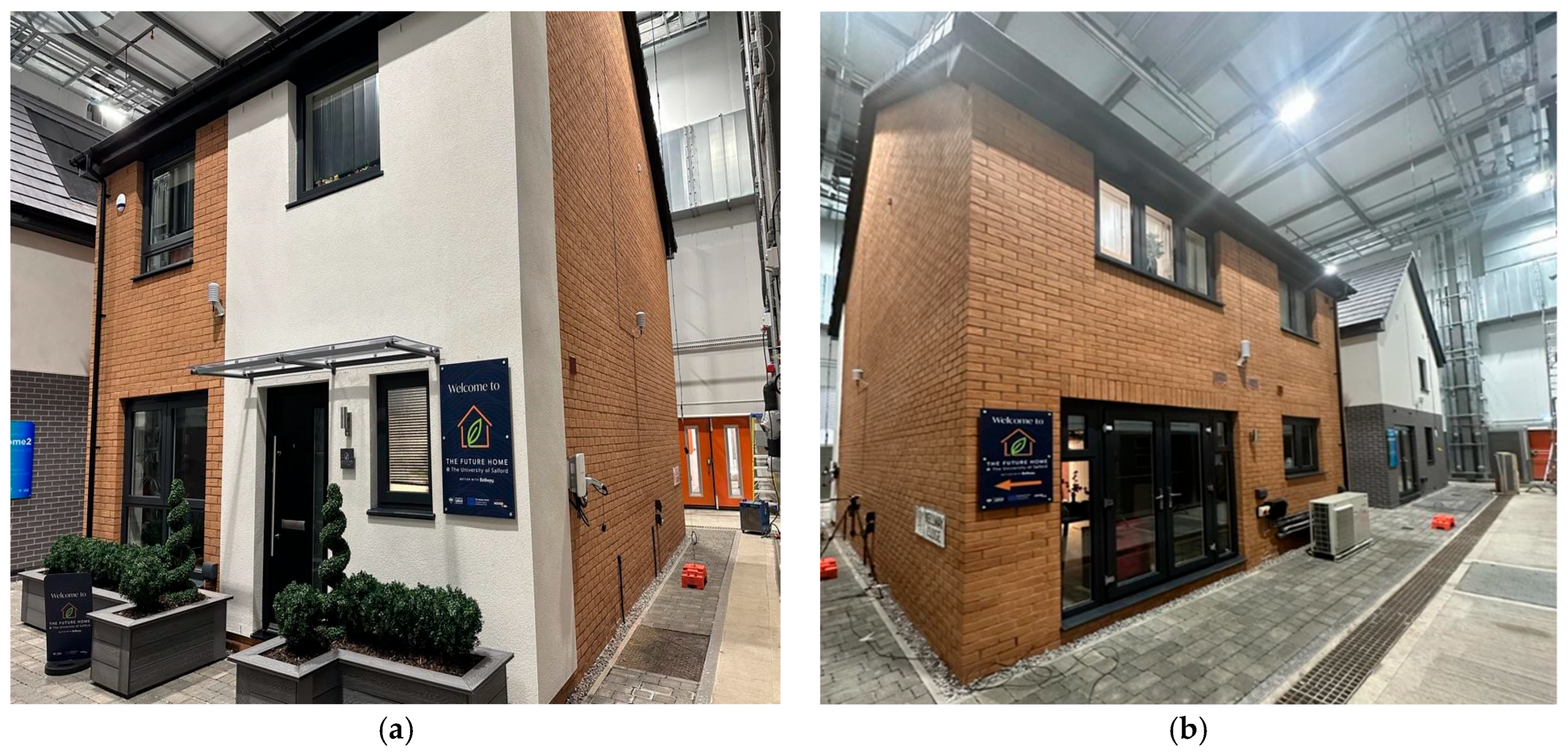
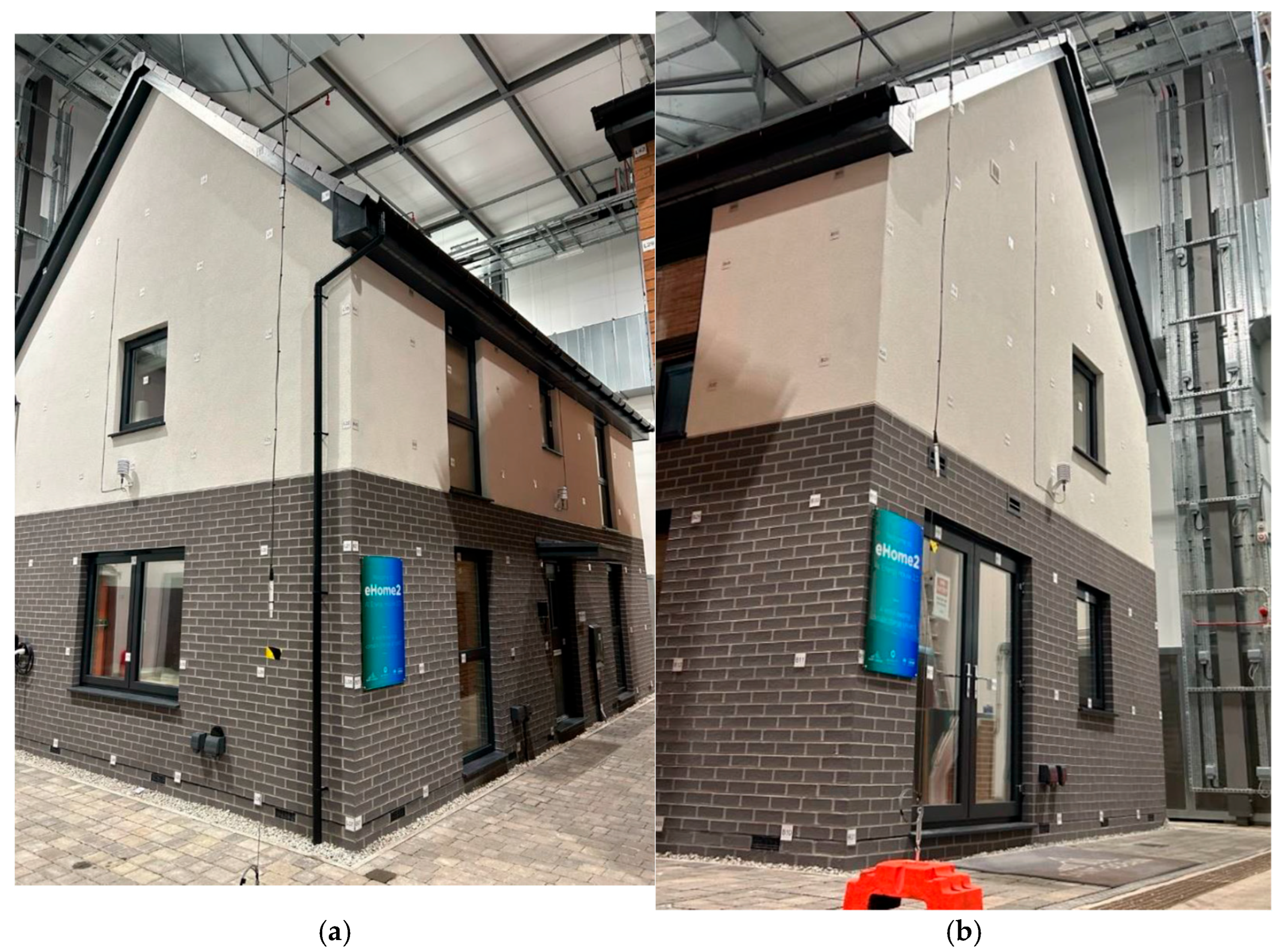
2.1. Introduction to Case Studies

Two test homes, “The Future Home” (TFH) built by Bellway and “eHome2” built by Saint-Gobain and Barratt, were used as case studies for this research. Both homes are timber-framed detached houses, with eHome2 using a closed panel system and TFH a closed panel timber frame. They incorporate renewable heating technologies and were designed to exceed the UK’s proposed Future Homes Standard (FHS). The homes were constructed and tested in the controlled environmental chamber of Energy House 2.0, minimising external variables such as weather and enabling highly accurate measurements. This study was part of a Future Homes project, funded by Innovate UK, which aims to create a globally competitive centre for research and innovation in net zero housing in Greater Manchester. For the detailed measured fabric performances, please refer to the TFH [40] and eHome2 [41] reports.

2.2. DTS and SAP Models

DesignBuilder (v7.3.0.044), incorporating EnergyPlus (v9.4) as its physics engine, was used to develop the DTS models due to its capability to model complex interactions within building systems dynamically [38]. In contrast, Standard Assessment Procedure (SAP) is a steady-state model and currently operates on version SAP 10.2 [5]; it has long been used as the official methodology used in the UK for assessing and comparing the regulatory energy and environmental performance of domestic buildings. SAP employs a bottom-up approach to derive the HTC by aggregating the W/K losses, while DTS models simulate the aggregate heat loss test on an hourly basis. For the detailed development of SAP models, please refer to the TFH [40] and eHome2 [41] reports.

2.3. Geometric Modelling

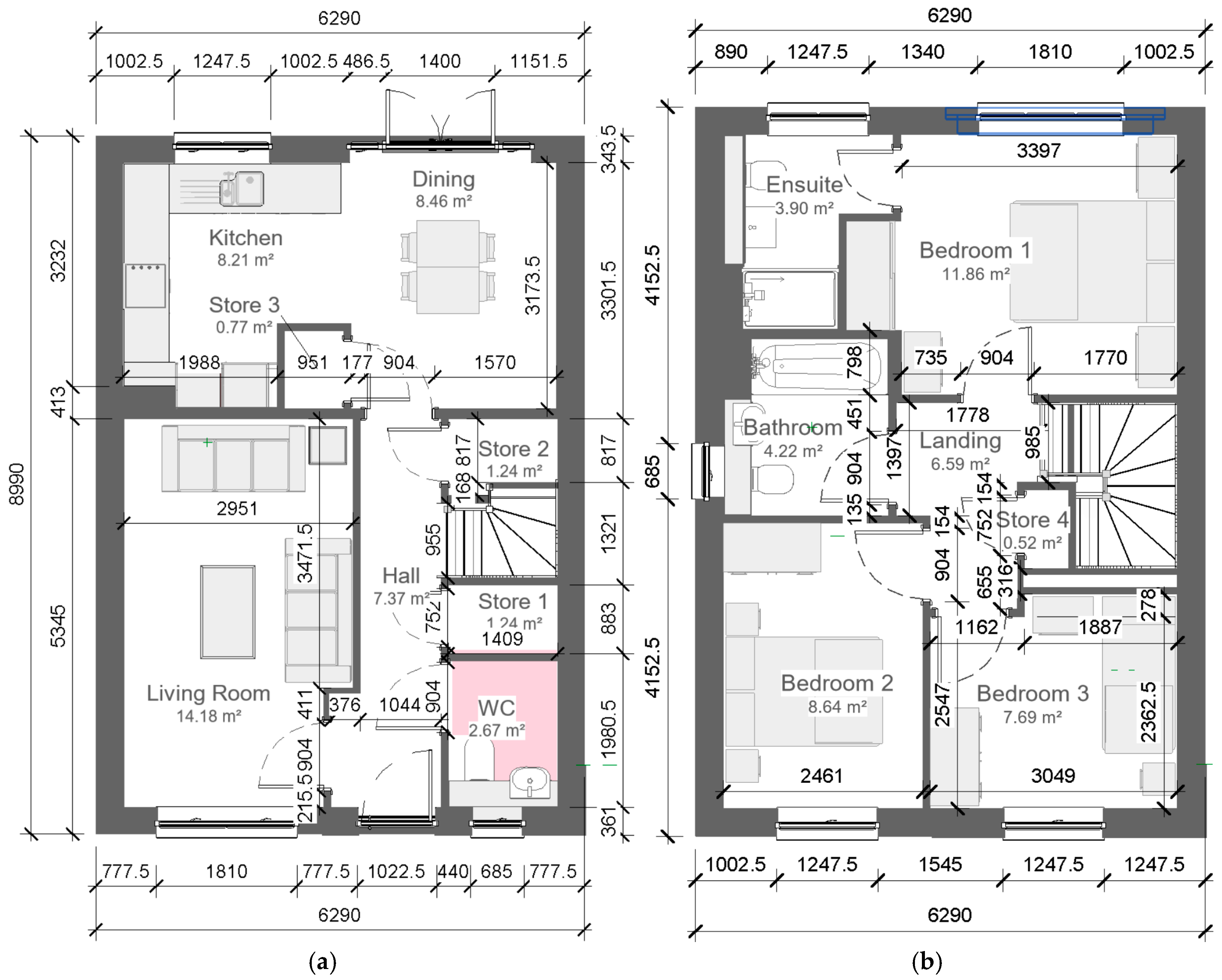
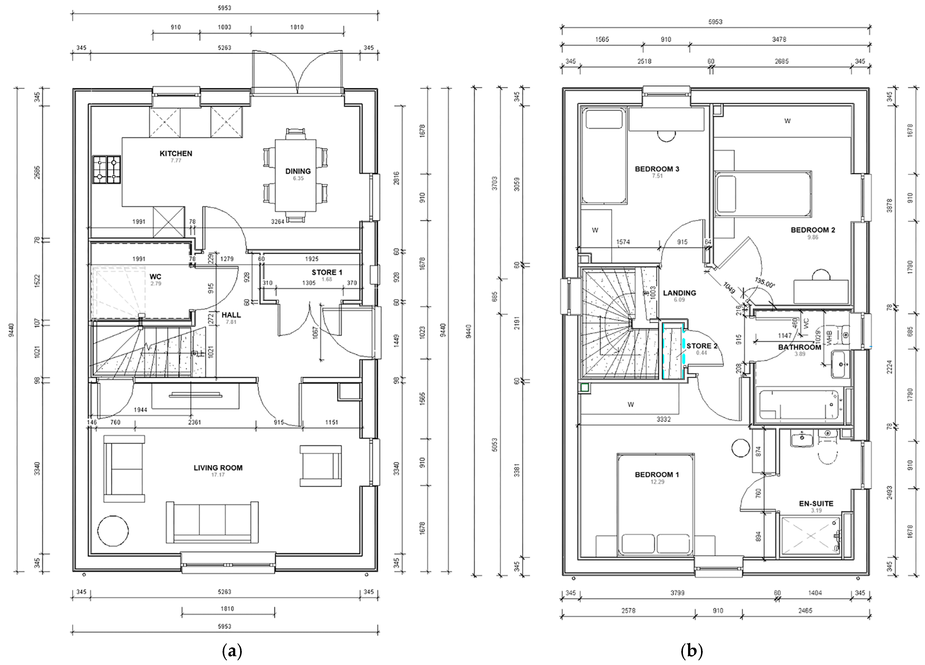
2.3.1. Floor Plans and General Description

Figure 1a,b show the front and rear elevations of TFH, respectively, while Figure 2a,b show the front and rear elevations of eHome2. Both are three-bedroom detached houses, including a kitchen diner, living room, bathroom, ensuite, toilet and three bedrooms, designed to meet the UK’s anticipated FHS. The floor plan provided modellers with the necessary resources to create DTS models for TFH (Figure 3a,b) and eHome2 (Figure 4a,b). Please refer to the Supplementary Files for more detailed geometric information (Tables S1–S3), comprehensive elevation plans (Figures S2 and S3), and window dimensions (Tables S4 and S5).

2.3.2. Differences in Floor Area and Ceiling Heights Between DTS and SAP

Figure 5 shows the DTS model rendered in DesignBuilder replicating the TFH and eHome2. Table 1 presents a detailed breakdown of the defined thermal zones, illustrating that the total floor area measures 88.49 m2 for TFH and 86.64 m2 for eHome2. In contrast, the SAP calculations indicate a total floor area of 92.82 m2 for TFH and 91.26 m2 for eHome2. This discrepancy arises from the DesignBuilder model’s inclusion of cupboards, storerooms, and internal partitions in its calculations. Additionally, for SAP calculations, the ground floor ceiling height is 2.39 m in TFH and 2.32 m in eHome2, while on the first floor, it is 2.69 m for TFH and 2.61 m for eHome2. For DesignBuilder, it has the same ground floor ceiling height with SAP but for the first floor it is 2.35 m for TFH and 2.30 m as the internal floor thickness (0.34 m for TFH and 0.31 m for eHome2), which was taken into account. The roof pitch is 35 degrees for TFH and 45 degrees for eHome2.

2.3.3. Definition of Zones, Blocks, Surfaces and Loft Hatch

In this study, blocks are drawn using outer dimensions. The loft hatch was modelled by specifying its construction materials and insulation levels, while a stairwell was incorporated to connect the ground floor to the first floor, necessitating the creation of an opening that merged the “Landing” and “Hall” spaces.

2.4. Construction Details

2.4.1. U-Values

This section presents the key thermal properties affecting the designed and model-predicted HTC. Table 2 presents the detailed construction specifications, including layer-by-layer material thickness and conductivity, and cavity specifications, for TFH and eHome2. A detailed breakdown of all construction materials and layers is provided in the Supplementary Material (Tables S6–S20). Table 3 presents a comparison of the design parameters for TFH, eHome2 and FHS [2]. In terms of external wall U-values, both TFH and FHS align at 0.18 W/m2K for brick walls, whereas eHome2 demonstrates greater efficiency with a lower U-value of 0.13 W/m2K. A similar trend is observed for rendered walls. For loft ceiling U-values, TFH performs better at 0.09 W/m2K, surpassing both eHome2 and the FHS benchmark of 0.11 W/m2K. When examining the ground floor U-value, both TFH and eHome2 meet the FHS standard of 0.13 W/m2K with a more efficient value of 0.11 W/m2K. Window U-values (including frames) for both homes, based on manufacturer specifications, are consistent with the FHS standard of 1.2 W/m2K. The FHS does not specify a limiting U-values for internal partitions, floors, and doors.

2.4.2. Thermal Bridging Inputs

Thermal bridges for both homes were modelled using TRISCO software [42], with detailed calculations available in the TFH [40] and eHome2 [41] reports. The y-value, an indicator of thermal bridging heat loss, can be determined by dividing the thermal bridging heat transfer coefficient by the total area of the home’s exposed elements. Both TFH and eHome2 achieve a calculated y-value of 0.05, meeting the FHS requirement [2]. DesignBuilder software facilitates the modelling of linear thermal bridging at various junctions by allowing users to input psi-values in the linear thermal bridges at the junctions section under the Construction tab; these data are illustrated in Table 4.

2.4.3. Roof Ventilation, Ground Temperature and Sub-Floor Voids

While the models are already highly detailed, certain additional modelling parameters warrant particular attention. Previous studies have emphasised the importance of elements such as roof ventilation, ground temperature, and sub-floor void modelling [7,28]. Incorporating these could substantially improve model accuracy and thermal performance representation.
The loft space was modelled as a semi-exterior, unconditioned zone in DesignBuilder, with an assumed ventilation rate of 0 Air Changes per Hour (ACH) of the cold roof, as the roof’s air tightness tab was disabled. However, the eHome2 report indicates that the roof features ventilation through soffit vents and a ventilated ridge [41], while the TFH report specifies the use of over fascia vents and a vented ridge tile system [40]. Therefore, it is expected that the roof incorporates some form of intended ventilation. Previous studies have highlighted the significance of modelling roof ventilation. Sanders et al. established guidelines from 80 properties, finding unventilated lofts’ ventilation rates roughly equalled wind speed (m/s) [43]. Applying these guidelines, Beizaee estimated loft ventilation rates for average wind speeds of 2.7–4.0 m/s, yielding 2.7–4.0 ACH in unventilated lofts in the study [7]. For ventilated lofts, Allinson examined UK pitched roofs under low wind speed conditions [44], proposing a ventilation rate of 2 ACH based on assumptions established by Burch [45]. Given that both homes are situated in an environmental chamber with low wind speed (0.2 m/s) and feature ventilated lofts, their conditions align with Allinson’s study; consequently, a ventilation rate of 2 ACH is applied in this study.
DesignBuilder’s default ground temperature is set at 18 °C, primarily suited for large non-residential buildings. However, ground temperatures beneath homes differ significantly. For residential structures, the actual ground temperature typically lies between the undisturbed soil temperature and the home’s average internal temperature [38]. In this study, during the aggregate heat loss testing period at Energy House 2.0, measurements indicated that the average ground floor temperature was 10.1 °C for TFH and 9.5 °C for eHome2 [40,41]. Ground floor temperatures were measured using soil sensors located approximately 1 m belowground under TFH and eHome2.
When modelling ground floors in DesignBuilder, the default setting assumes a single layer in direct contact with the soil [38]. While this configuration can be modified, it may not accurately represent real-world conditions. In reality, suspended concrete floors often have an air void between the floor and the soil, altering the heat transfer mechanism. This arrangement results in heat loss occurring through the suspended floor to the void and then to the soil, rather than directly from floor to soil as modelled. Previous studies have investigated this discrepancy and its impact on thermal performance calculations [7,28]. Therefore, this calibration step will include modelling the sub-floor void with a depth of 150 mm, along with the below-grade walls. The sub-floor void ground floor is in touch with the ground soil; it is set to a construction in DesignBuilder with thickness 0.5 m and conductivity of 1.2 W/mK. The below-grade walls were made of 0.14 m aerated concrete block (λ = 0.24 W/mK), 0.072 m of Knauf insulation Dri Therm (λ = 0.038 W/mK) and another 0.1 m of aerated concrete block.

2.5. Weather File Adjustments—Controlled Chamber Conditions

The weather file was modified to reflect the test conditions (Table 5). The EnergyPlus IWEC weather file served as the base [46], with modifications for the dates from 1 Jan to 8 Jan to mirror the aggregate heat loss environment. During these eight days, the recorded temperature was 5.2 °C (day 2 and 4) and 5.3 °C (day 1, 3 and 5–8), and the relative humidity was 81% (Table 5); see the Supplementary Material (Tables S21 and S22) for additional information. The dew-point temperature, though not directly measured, was calculated using the measured dry-bulb temperature and relative humidity using the psychrometric chart [47]. Additionally, solar radiation variables were reduced to zero in the weather files to match the absence of these elements in the controlled test chambers. The atmospheric pressure inside the chamber was maintained at a constant of 101,325 Pa, which corresponds to standard atmospheric pressure at sea level [47]. Opaque Sky Cover represents the fraction of the sky covered by dense clouds that block sunlight, while Total Sky Cover includes all types of clouds, both measured in tenths. In an environmental chamber modelled in EnergyPlus, these values are set to zero to ensure a controlled, consistent environment without cloud-induced variability. Also, snow depth and liquid precipitation depth are set to 0 to eliminate the influence of external precipitation factors. The horizontal infrared radiation (IRH) is determined using Equation (1) and the sky emissivity from Equation (2). Assuming a sky emissivity of 0.793 and N being 0, when the dry-bulb temperature is 5.2 °C, the IRH is 269.59 W/m2. At a dry-bulb temperature of 5.3 °C, the IRH increases slightly to 269.87 W/m2. The wind speed was measured in the chamber to be a constant 0.2 m/s.
I R H = ε σ T 4 ,
where IRH = Horizontal Infrared Radiation Intensity (W/m2), ε = sky emissivity = 1, σ = Stefan-Boltzmann constant = 5.6697 × 10⁻⁸ W/(m2K4) and T = dry-bulb temperature in Kelvin.
ε = ( 0.787 + 0.764 ln T d 273 1 + 0.0224 N 0.0035 N 2 + 0.00028 N 3
where Td is the dewpoint temperature (K), N is the opaque sky cover (tenths),

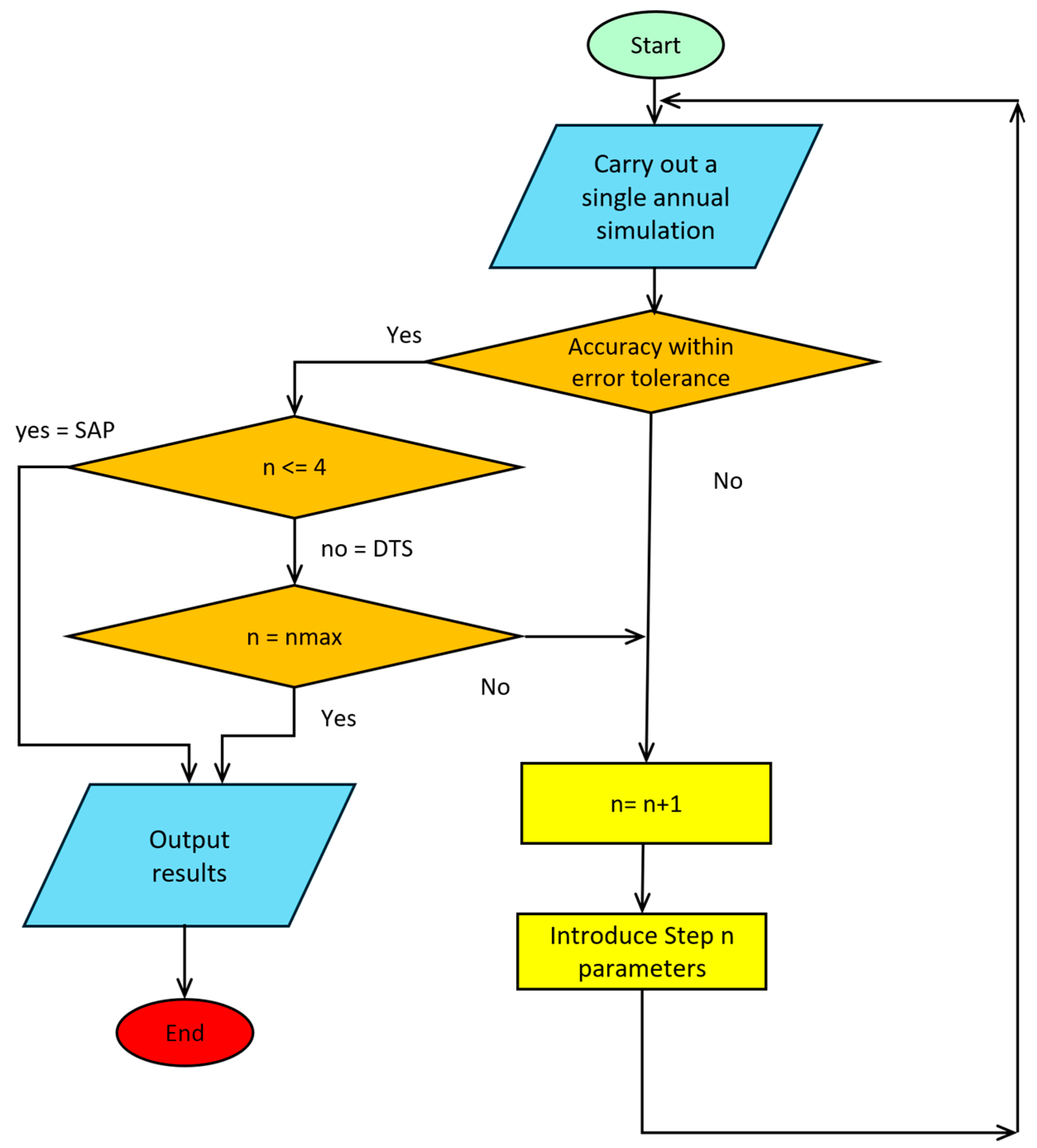
2.6. Development of Calibration Procedure

The values selected for weather file parameters were chosen to accurately replicate the controlled environment conditions within Energy House 2.0 during the aggregate heat loss test. To setup an aggregate heat loss test in DesignBuilder, the first step involved eliminating occupancy and scheduling and all internal gains (including equipment and hot water), ensuring each thermal zone was declared as having no activity, with occupancy density at zero and occupancy scheduling set to off. Lighting was set to be permanently off, and natural ventilation was excluded as all internal doors were closed. The heating schedule was assumed to be on for 24 h with a set-point of 21 °C, using electric convectors with a COP of 1.0, to maintain consistency with the conditions during the aggregate heat loss test.
Initial values for key parameters such as U-values and air permeability rates were taken from design documentation and manufacturer data. Following construction, these values were updated with measured as-built data, as described below, to ensure the simulation matched the actual building performance. Table 6 provides a comparison between the design and as-built values for various building fabric parameters of TFH and eHome2. The U-values for both homes were determined using a network of heat flux plates (HFPs). These measurement locations were selected through preliminary thermographic analysis to capture both thermally bridged and non-bridged sections of the building envelope. The HFPs were installed in 3 × 3 grid arrangements across ceiling, floor, and wall surfaces using thermal contact paste and adhesive tape to ensure proper thermal coupling. For each element, the U-value was calculated as a weighted average of the grid readings, with 15% weight assigned to the timber/stud locations and 85% to the insulated panel areas, following BR443 conventions [48]. For each measurement point, the temperature gradient was established by recording the adjacent internal and external air temperatures [49]. Note that for internal partition, floor and door U-value, they were measured by creating a temperature difference between two zones of interest and measuring the heat loss with HFPs. The air permeability rates for both homes were evaluated through standardised air permeability testing protocols, i.e., ATTMA Technical Standard L1 protocols [50]. This assessment was conducted under controlled conditions where all intentional ventilation pathways were temporarily sealed, and a reference pressure differential of 50 pascals was established across the building envelope [50]. The “Point Thermal Transmittance” (PTT) metric is employed for ground floors instead of U-values, as it accounts for various influencing factors such as thermal bridging, air brick impact, perimeter effect and insulation geometry [40,41]. PTT-values are reported as ranges rather than averages to address the limitations of comparing average HFPs measurements to design U-values. The whole-house HTC was measured using aggregate heat loss test, following the “Whole-House Heat Loss Test Method (Coheating)” developed by Johnston et al. [26]. This post-construction technique involves maintaining the unoccupied building at a consistent internal temperature while measuring the energy input required to sustain these conditions. It enables quantification of the combined thermal losses occurring through the various building elements including walls, floors, roofing systems, doors, and windows [26,51].
Table 7 outlines the calibration steps, including the in situ measurement updates for steps 2–4 and the modelling details updates for steps 5–8. Calibration steps 1–4 were conducted for both DesignBuilder (DTS) and SAP models, while steps 5–8 were carried out solely for DesignBuilder (DTS) models. Figure 6 serves as a visual flowchart summary of the overall calibration workflow. After each simulation, model accuracy is checked against the error tolerance. If not met, additional modelling parameters are introduced, and n (the calibration step) is incremented. Calibration ends when tolerance is achieved or n reaches its maximum value (nmax). Results are then output.

3. Results

Table 8 below presents a comparison of the measured, model-predicted, and design HTC values for TFH and eHome2, using the aggregate heat loss test, simulated aggregate heat loss test in the DTS, and SAP model, respectively. The measured HTC values from aggregate heat loss tests were 82.2 (±1.8) W/K for TFH and 76.7 (±2.01) W/K for eHome2.
In Step 1, the HTC model predicted by the DTS model for TFH showed a thermal performance gap of 6.8 W/K lower than the measured value. This 6.0% difference highlights the importance of post-construction evaluations. Applying as-built U-values (step 2) increased the model-predicted HTC by 2.7 W/K, mainly due to higher loft U-values and ground floor PTT-values. Incorporating as-built air permeability (step 3) further increased model-predicted HTC by 4.8 W/K. This increase was greater than the U-value impact, as the actual air permeability was 1.6 times higher than the design value. In step 4, the model-predicted HTC aligned closely with aggregate heat loss test results, with just a 2.1 W/K overprediction. The total of the model-predicted HTC increases of 7.5 W/K was the sum of the adjustments from U-values and air permeability. Regarding the initial (step 1) design HTC calculated by the SAP model for TFH, the difference was just 0.3 W/K compared with the model-predicted HTC. SAP showed more sensitivity to air permeability, with a 5.4 W/K increase in HTC versus the DTS model’s 4.8 W/K.
For eHome2, the trend differed. As-built U-values increased model-predicted HTC by 5.7 W/K, as these values exceeded the design specifications, particularly in external walls. Using as-built air permeability reduced model-predicted HTC by 0.6 W/K because the measured air permeability was lower than the design value, which contrasts with the TFH results. The combined impact of as-built U-values and air permeability led to a 5.1 W/K increase in model-predicted HTC, with the change in U-values playing a larger role. Additionally, SAP’s design HTC differed from DTS predictions by 1.3 W/K, a larger gap than TFH. In the eHome2 case, SAP demonstrated greater sensitivity to U-values, with an increase in HTC of 6.9 W/K compared to the DTS model’s 5.7 W/K.
Additional modelling parameters (step 5–8) were taken to calibrate the model-predicted HTC from the DTS simulation of the aggregate heat loss test. Changing the roof ventilation had a minimal effect on the model-predicted HTC for both houses, reducing it by just 0.1 W/K. This may be due to the highly insulated lofts which decouple roof ventilation from the indoor air. Adjusting ground temperatures led to an HTC increase of 3.9 W/K for TFH and 4.1 W/K for eHome2, as actual ground temperatures were lower than had been assumed; this indicates that ground temperature was a significant source of discrepancy pre-calibration. Sub-floor void modelling reduced HTC by 4.2 W/K for TFH and 4 W/K for eHome2, as the air void increased thermal resistance between the floor and soil. This suggests that default DesignBuilder settings may overestimate heat loss without more detailed sub-floor void modelling.
When all refinements were applied, the DTS models closely matched the aggregate heat loss test results. The final DTS predictions differed by just 0.4 W/K (0.5%) for TFH and 0.5 W/K (0.6%) for eHome2. This is a much smaller thermal performance gap than SAP models, which could not include the additional calibration steps. The SAP design HTC values showed greater discrepancies with the measured HTC, with differences of 2.6% for TFH and 4.3% for eHome2 (Table 8).

4. Discussion

The final DTS model-predicted HTC results demonstrate a high level of accuracy, with differences from measured HTC of only 0.5% for TFH and 0.6% for eHome2. These differences fall within the aggregate heat loss test uncertainty range; the aggregate heat loss test itself had an uncertainty range of ±2.19% for TFH and ±2.62% for eHome2. These uncertainties were lower than the uncertainty reported by other studies (±8%), such as in Jack et al. [52], due to the controlled testing environment. As discussed in the introduction, the smallest previously reported performance gap was 2.4% by Marshall et al. [28], with typical performance gaps being much higher [4,29,30]. Consequently, to the authors’ knowledge, this study achieves the smallest performance gap and highest modelling accuracy in the field to date and highlights the value of controlled environmental chambers in reducing uncertainty in measurement. While such facilities are not widely accessible, these results provide a benchmark for best-case model calibration and can inform improvements in field-based studies. However, it should be noted that close agreement in HTC values does not necessarily validate all individual assumptions within the model, as different parameter combinations can yield similar HTC results. Future work will therefore focus on sensitivity analysis to more robustly identify the influence of specific model parameters and further refine the calibration process.
The SAP design HTC results, even when using as-built U-values and air permeability, did not provide results with the same accuracy as the DTS. The model-predicted HTC by DTS models was more accurate than SAP design HTC for two homes. The discrepancies between SAP and DTS models stem from their distinct methodologies, with DTS offering greater customisation for detailed modelling, highlighting SAP’s limitations in this regard. It is hoped that the precise geometrical and construction details provided in this paper will enable other modellers to test other DTS models, such as EnergyPlus [53], IES [54] or TRNSYS [55]. Utilising these openly accessible floor plans allows for the theoretical generation of similar outputs across different modelling efforts [51,56].
The UK government plan to move to dynamic Home Energy Model (HEM) from steady-state SAP models [1]. Thus, if the results are generalisable to a wider set of houses, it supports the value of a transition from SAP to HEM. HEM could incorporate options for detailed modelling of sub-floor voids in suspended floor constructions and allow for different ground floor temperature inputs. It will be useful to implement the simulated aggregate heat loss tests in HEM to allow easy comparison of model-predicted with measured HTC in future studies. More accurate assessment of energy performance, as enabled by DTS models in this paper, is essential to ensure that policy targets for zero carbon homes are achieved in reality, not just in regulatory calculations. This transition supports not only compliance but also builds confidence among policymakers, industry, and homeowners in the reliability of projected energy and carbon savings.
This study found that achieving the best results, where model-predicted HTC matches the aggregate heat loss test, requires accurate as-built U-values, as-built air permeability, and modelling of roof ventilation, ground floor, and sub-floor void. In the context of newly built homes with unoccupied loft spaces and high levels of loft insulation, this study indicates that the specific value of the roof ventilation rate has minimal impact. However, this finding may not extend to older buildings lacking loft insulation, warranting further investigation into the effects of roof ventilation in less insulated structures. While measuring ground floor temperatures in homes can be challenging, modellers can reference Met Office data [57] or use 10 °C in this study measured during testing with average UK winter temperature (5.3 °C). Modelling the sub-floor void was found to be crucial in this study, significantly affecting HTC predictions and potentially indicating lower model-predicted heat loss in suspended floor constructions.
The environmental chamber used in this study eliminates uncertainties, such as solar radiation and wind, yielding highly accurate aggregate heat loss test results. Both homes in this study exhibit significant differences when as-built U-values are employed, aligning with Johnston et al.’s findings that U-value discrepancies in newly built houses are a primary cause of large variations in HTC [4]. Moreover, the magnitude of change observed in calibration steps 2 and 3 (employing as-built values) varied between TFH and eHome2. This variation suggests that construction quality’s impact on thermal performance can differ substantially between buildings, even within the same project. Such observations underscore the necessity for individual building assessment rather than sole reliance on standardised assumptions in thermal performance evaluations, as models are only as good as their inputs. While heat flux plates and air permeability tests offer high accuracy, portable U-value kits and quick air permeability assessments can provide alternative methods for obtaining as-built values. However, aggregate heat loss tests are expensive and require empty rooms. Alternative commercial methods like QUB offer faster testing with reduced accuracy. The application of SMETER methods [58] is likely to make measured HTC much more commonplace in future. The use of Energy House 2.0 means any of these methods can be completed in a very short time.
The calibration framework presented here could, in principle, be extended to multi-zone or more complex buildings using similar DTS modelling approaches. However, additional challenges would include the allocation of appropriate heating power across different rooms and the increased complexity of modelling internal heat transfer dynamics. Larger buildings may require more detailed input data and calibration for each zone to maintain accuracy.
This study demonstrates the feasibility of precise whole-house HTC calibration under steady-state conditions. As part of the ongoing Future Homes project, subsequent phases will expand the scope of investigation. The Energy House 2.0 facility will host testing of heating systems, ventilation, domestic hot water, smart systems, etc., for both TFH and eHome2. These tests will form the basis for future modelling and calibration efforts, extending beyond the current study’s steady-state fabric focus to encompass dynamic conditions and system interactions. The calibrated model developed in this study offers significant potential for further research applications. The authors will utilise this calibrated model as a foundation for advanced calibration using data from the Future Homes project in the future.
In the broader policy context, the FHS is set to become mandatory in the UK and will require all new homes to be zero carbon ready, meaning they will achieve zero carbon emissions once the electricity grid is fully decarbonised. Utilising TFH and eHome2 within the controlled environment of Energy House 2.0 ensures that the results are representative of new-build homes in the UK, although it should be noted that controlled chamber conditions do not capture all real-world variables, such as occupant behaviour and weather. Even so, the controlled environment provides a valuable best-case benchmark for homes built to the FHS. The calibration method described here could also be adapted for in-use settings by incorporating measured data from occupied buildings and accounting for real-world variability. Future work will include sensitivity analysis to identify which input parameters most influence calibration accuracy, as suggested by recent studies [59,60,61]. In addition, integrating calibrated models into building design workflows and exploring advanced approaches, such as physics-informed neural networks (PINNs), for improved simulation and regulatory assessment will be valuable directions for further research [62].
The current open access dataset is primarily intended to support HTC calibration and benchmarking. Future updates will include annual simulation results using DesignBuilder’s default occupancy and operational schedules, making it a more versatile resource for researchers interested in annual performance and facilitating integration with existing building performance assessment workflows.

5. Conclusions

This study demonstrates an accurate calibration methodology for using DTS models to predict whole-house HTC under steady-state conditions. By systematically incorporating as-built measurements and modelling refinements, the research achieved a high level of accuracy in closing the thermal performance gap between model-predicted and measured HTCs for two zero carbon ready homes: TFH and eHome2.
The main findings of this paper can be summarised as follows, where the first bullet point below answers the first research question, the second and third bullet points answer the second research question, and the last two bullet point answers the third research question:
  • Incorporating as-built U-values and air permeability rates significantly improved model accuracy, with their relative impact varying between the two houses.
  • The calibrated DTS models achieved remarkably low performance gaps of 0.5% for TFH and 0.6% for eHome2, falling within the uncertainty range of aggregate heat loss test measurements.
  • DTS models outperformed SAP calculations in accuracy, supporting the UK’s planned transition to more dynamic assessment methods.
  • Modelling sub-floor voids in suspended floor constructions substantially affected HTC predictions, indicating lower heat loss than previously assumed.
  • Roof ventilation rates had minimal impact on HTC for these highly insulated homes, but may be more significant for older, less insulated buildings.
This study demonstrates the feasibility of precise whole-house HTC calibration under steady-state conditions, surpassing previous calibration efforts in the literature. The open access of the calibrated models and methodology provides a valuable resource for future research in building energy performance. Freely available datasets enable academics to replicate and extend the analysis, support policymakers in developing and validating energy standards, and offer software developers robust test cases for tool innovation. The findings support the transition from steady-state to dynamic modelling approaches in building energy assessments. The unique contribution of this work is the reduced uncertainty of the results achieved under a controlled environment in Energy House 2.0 environmental chambers. Future work will include uncertainty analysis, such as Monte Carlo or sensitivity analysis, to further substantiate the robustness of the calibration results.

Supplementary Materials

The following supporting information can be downloaded at: https://www.mdpi.com/article/10.3390/su17156673/s1: Please refer to Tables S1–S3 for more detailed geometric information, Figures S1–S3 for comprehensive elevation plans, and Tables S4 and S5 for window dimensions. A detailed breakdown of all construction materials and layers is provided in Tables S6–S20. Additional information on Chamber conditions is provided in Tables S21 and S22.

Author Contributions

Conceptualization, C.T., R.F., X.Z., G.H., D.F. and D.A.; methodology, C.T., R.F., X.Z., G.H., H.P.D.-H., D.F., D.A. and M.D.; software, C.T., X.Z. and A.S.; validation, C.T., X.Z., G.H., H.P.D.-H. and D.A.; formal analysis, C.T., R.F., X.Z., G.H., H.P.D.-H. and D.F.; investigation, C.T., R.F., X.Z., G.H., H.P.D.-H., D.F. and A.S.; resources, R.F.; data curation, C.T., X.Z., G.H., H.P.D.-H. and A.S.; writing—original draft preparation, C.T., R.F., X.Z., G.H., D.A. and M.D.; writing—review and editing, C.T., R.F., X.Z., G.H., H.P.D.-H., D.F., D.A., M.D., L.J. and W.S.; visualization, C.T., X.Z., G.H., H.P.D.-H. and A.S.; supervision, R.F., D.F., D.A. and L.J.; project administration, R.F., L.J. and W.S.; funding acquisition, R.F. and W.S. All authors have read and agreed to the published version of the manuscript.

Funding

This work was conducted as part of a Future Homes initiative, funded by Innovate UK Application Number 10054845, which strives to establish a globally competitive hub for research and innovation in net zero housing within Greater Manchester. The project represents a collaborative effort between Barratt Developments, Bellway Homes, the Energy Innovation Agency, Q-bot, RED Cooperative, RSK Environment, Saint-Gobain, the University of Manchester, and the University of Salford. The APC was funded by the University of Salford.

Institutional Review Board Statement

Not applicable.

Informed Consent Statement

Not applicable.

Data Availability Statement

Data supporting this study are openly available from University of Salford Repository (USIR) at DOI: https://doi.org/10.17866/rd.salford.28473599 (accessed on 1 June 2025).

Conflicts of Interest

The authors declare no conflicts of interest. The funders had no role in the design of the study; in the collection, analyses, or interpretation of data; in the writing of the manuscript; or in the decision to publish the results.

Abbreviations

The following abbreviations are used in this manuscript:
FHSFuture Homes Standard
HTCHeat Transfer Coefficient
DTSDynamic Thermal Simulation
SAPStandard Assessment Procedure
TFHThe Future Home in Energy House Labs Environmental Chamber 1 developed in collaboration between Bellway Homes and the University of Salford
eHome2Experimental house in Energy House Labs Environmental Chamber 1 developed in collaboration between Barratt Developments, Saint-Gobain, and the University of Salford
PTTPoint Thermal Transmittance
LoDLevel of Detail
HEMHome Energy Model
EPCEnergy Performance Certificate
HFPHeat Flux Plates
USIRUniversity of Salford Institutional Repository

References

  1. Home Energy Model: Future Homes Standard Assessment. Available online: https://www.gov.uk/government/consultations/home-energy-model-future-homes-standard-assessment (accessed on 30 September 2024).
  2. HM Government. The Future Homes and Buildings Standards: 2023 Consultation; Department for Levelling Up, Housing and Communities: London, UK, 2023. [Google Scholar]
  3. HM Government. Climate Change Act 2008; Statute Law Database; HM Government: London, UK, 2008. [Google Scholar]
  4. Johnston, D.; Miles-Shenton, D.; Farmer, D. Quantifying the Domestic Building Fabric ‘Performance Gap. Build. Serv. Eng. Res. Technol. 2015, 36, 614–627. [Google Scholar] [CrossRef]
  5. HM Government BEIS. SAP 10.2: The Government’s Standard Assessment Procedure for Energy Rating of Dwellings; BRE Garston: Watford, UK, 2023. [Google Scholar]
  6. BS EN 17887-1:2024; Thermal Performance of Buildings. In Situ Testing of Completed Buildings. Data Collection for Aggregate Heat Loss Test (Part 1). BSI: London, UK, 2024.
  7. Beizaee, A. Measuring and Modelling the Energy Demand Reduction Potential of Using Zonal Space Heating Control in a UK Home. Ph.D. Thesis, Loughborough University, Loughborough, UK, 2016. [Google Scholar]
  8. Bou-Saada, T.E.; Haberl, J.S. An Improved Procedure for Developing Calibrated Hourly Simulation Models. In Proceedings of the Building Simulation 1995: 4th Conference of IBPSA, Madison, WI, USA, 14–16 August 1995; pp. 475–484. [Google Scholar]
  9. Coakley, D.; Raftery, P.; Keane, M. A Review of Methods to Match Building Energy Simulation Models to Measured Data. Renew. Sustain. Energy Rev. 2014, 37, 123–141. [Google Scholar] [CrossRef]
  10. Georgiou, G.; Eftekhari, M.; Eames, P. Calibration and Validation of Residential Buildings: 8 Case Studies of Detached Houses; IBPSA: Las Cruces, NM, USA, 2013. [Google Scholar]
  11. Marini, D.; Webb, L.H.; Diamantis, G.; Buswell, R.A. Exploring the Impact of Model Calibration on Estimating Energy Savings Through Better Space Heating Control. In Proceedings of the Building Simulation and Optimization: Second Conference of IBPSA-England Conference, UCL, London, UK, 10–11 June 2014. [Google Scholar]
  12. Mustafaraj, G.; Marini, D.; Costa, A.; Keane, M. Model Calibration for Building Energy Efficiency Simulation. Appl. Energy 2014, 130, 72–85. [Google Scholar] [CrossRef]
  13. Yoon, J.; Lee, E.J.; Claridge, D.E. Calibration Procedure for Energy Performance Simulation of a Commercial Building. J. Sol. Energy Eng. Trans. ASME 2003, 125, 251–257. [Google Scholar] [CrossRef]
  14. Reddy, T. Literature Review on Calibration of Building Energy Simulation Programs: Uses, Problems, Procedures, Uncertainty and Tools. ASHRAE Trans. 2006, 112, 226–240. [Google Scholar]
  15. Gillich, A.; Saber, E.M.; Mohareb, E. Limits and Uncertainty for Energy Efficiency in the UK Housing Stock. Energy Policy 2019, 133, 110889. [Google Scholar] [CrossRef]
  16. De Wilde, P.; Tian, W. Towards Probabilistic Performance Metrics for Climate Change Impact Studies. Energy Build. 2011, 43, 3013–3018. [Google Scholar] [CrossRef]
  17. Srivastav, A.; Tewari, A.; Dong, B. Baseline Building Energy Modeling and Localized Uncertainty Quantification Using Gaussian Mixture Models. Energy Build. 2013, 65, 438–447. [Google Scholar] [CrossRef]
  18. Kumbaroglu, G.; Madlener, R. Evaluation of Economically Optimal Retrofit Investment Options for Energy Savings in Buildings. Energy Build. 2012, 49, 327–334. [Google Scholar] [CrossRef]
  19. Tian, W.; Heo, Y.; de Wilde, P.; Li, Z.; Yan, D.; Park, C.S.; Feng, X.; Augenbroe, G. A Review of Uncertainty Analysis in Building Energy Assessment. Renew. Sustain. Energy Rev. 2018, 93, 285–301. [Google Scholar] [CrossRef]
  20. Kershaw, T.; Eames, M.; Coley, D. Assessing the Risk of Climate Change for Buildings: A Comparison between Multi-Year and Probabilistic Reference Year Simulations. Build. Environ. 2011, 46, 1303–1308. [Google Scholar] [CrossRef]
  21. Jenkins, D.P.; Gul, M.; Patidar, S.; Banfill, P.F.G.; Gibson, G.; Menzies, G. Designing a Methodology for Integrating Industry Practice into a Probabilistic Overheating Tool for Future Building Performance. Energy Build. 2012, 54, 73–80. [Google Scholar] [CrossRef]
  22. Gaetani, I.; Hoes, P.-J.; Hensen, J.L.M. A Stepwise Approach for Assessing the Appropriate Occupant Behaviour Modelling in Building Performance Simulation. J. Build. Perform. Simul. 2020, 13, 362–377. [Google Scholar] [CrossRef]
  23. Yu, J.; Chang, W.-S.; Dong, Y. Building Energy Prediction Models and Related Uncertainties: A Review. Buildings 2022, 12, 1284. [Google Scholar] [CrossRef]
  24. Pan, Y.; Zhu, M.; Lv, Y.; Yang, Y.; Liang, Y.; Yin, R.; Yang, Y.; Jia, X.; Wang, X.; Zeng, F.; et al. Building Energy Simulation and Its Application for Building Performance Optimization: A Review of Methods, Tools, and Case Studies. Adv. Appl. Energy 2023, 10, 100135. [Google Scholar] [CrossRef]
  25. Belazi, W.; Ouldboukhitine, S.-E.; Chateauneuf, A.; Bouchair, A. Uncertainty Analysis of Occupant Behavior and Building Envelope Materials in Office Building Performance Simulation. J. Build. Eng. 2018, 19, 434–448. [Google Scholar] [CrossRef]
  26. Johnston, D.; Miles-Shenton, D.; Wingfield, J.; Farmer, D.; Bell, M. Whole House Heat Loss Test Method (Coheating); Leeds Metropolitan University: Leeds, UK, 2012. [Google Scholar]
  27. Parker, J.; Farmer, D.; Johnston, D.; Fletcher, M.; Thomas, F.; Gorse, C.; Stenlund, S. Measuring and Modelling Retrofit Fabric Performance in Solid Wall Conjoined Dwellings. Energy Build. 2019, 185, 49–65. [Google Scholar] [CrossRef]
  28. Marshall, A.; Fitton, R.; Swan, W.; Farmer, D.; Johnston, D.; Benjaber, M.; Ji, Y. Domestic Building Fabric Performance: Closing the Gap between the in Situ Measured and Modelled Performance. Energy Build. 2017, 150, 307–317. [Google Scholar] [CrossRef]
  29. Glew, D.; Collet, M.; Fletcher, M.; Hardy, A.; Jones, B.; Miles-Shenton, D.; Morland, K.; Parker, J.; Rakhshanbabanari, K.; Thomas, F.; et al. Demonstration of Energy Efficiency Potential (DEEP) Report 2.00 Case Studies Summary; Technical Report; Department for Energy Security and Net Zero and Department of Business, Energy and Industrial Strategy: London, UK, 2024. [Google Scholar]
  30. Farmer, D.; Henshaw, G.; Tsang, C.; Roberts, B.; Fitton, R.; Swan, W. DEEP Report 5.01 Salford Energy House Fabric Performance Testing; Department for Energy Security and Net Zero: London, UK, 2024. [Google Scholar]
  31. Jankovic, L.; Henshaw, G.; Tsang, C.; Zhang, X.; Fitton, R.; Swan, W. Heat Transfer Coefficient of a Building: A Constant with Limited Variability or Dynamically Variable? Energies 2025, 18, 2182. [Google Scholar] [CrossRef]
  32. Kolbe, T.H. Representing and Exchanging 3D City Models with CityGML. In 3D Geo-Information Sciences; Springer: Berlin/Heidelberg, Germany, 2009; pp. 15–31. [Google Scholar] [CrossRef]
  33. Gerrish, T.; Ruikar, K.; Cook, M.; Johnson, M.; Phillip, M. Using BIM Capabilities to Improve Existing Building Energy Modelling Practices. Eng. Constr. Archit. Manag. 2017, 24, 190–208. [Google Scholar] [CrossRef]
  34. Allen, E.A.; Pinney, A.A. Standard Dwellings for Modelling Details of Dimensions, Construction and Occupancy Schedules; Building Research Establishment: Watford, UK, 1990. [Google Scholar]
  35. Taylor, S.; Allinson, D.; Firth, S.; Lomas, K. Dynamic Energy Modelling of UK Housing: Evaluation of Alternative Approaches. In Proceedings of the 13th Conference of International Building Performance Simulation Association, Chambery, France, 25–28 August 2013; pp. 745–752. [Google Scholar]
  36. Monien, D.; Strzalka, A.; Koukofikis, A.; Coors, V.; Eicker, U. Comparison of Building Modelling Assumptions and Methods for Urban Scale Heat Demand Forecasting. Future Cities Environ. 2017, 3, 2. [Google Scholar] [CrossRef]
  37. Purdy, J.; Beausoleil-Morrison, I. The Significant Factors in Modelling Residential Buildings. In Proceedings of the 7th International Conference of the International Building Performance Simulation Association, Rio de Janeiro, Brazil, 13–15 August 2001; pp. 207–214. [Google Scholar]
  38. DesignBuilder Software Ltd. DesignBuilder; Version 7.3.0.044; DesignBuilder Software Ltd.: Stroud, UK, 2024. [Google Scholar]
  39. Tsang, C.; Fitton, R.; Zhang, X.; Henshaw, G.; Hernandez, H.D.; Farmer, D.; Allinson, D.; Dagli, M.; Jankovic, L.; Swan, W. Dataset for Article: “Calibration of Building Performance Simulations for Zero Carbon Ready Homes: Two Open Access Case Studies in Controlled Conditions”; School of Science, Engineering & Environment, University of Salford: Salford, UK, 2025. [Google Scholar]
  40. Fitton, R.; Diaz, H.; Farmer, D.; Henshaw, G.; Sitmalidis, A.; Swan, W. Bellway Homes “The Future Home” Baseline Performance Report; ERDF & Innovate: Salford, UK, 2024. [Google Scholar]
  41. Fitton, R.; Diaz, H.; Farmer, D.; Henshaw, G.; Sitmalidis, A.; Swan, W. Saint Gobain & Barratt Developments “eHome2” Baseline Performance Report; ERDF & Innovate: Salford, UK, 2024. [Google Scholar]
  42. Physibel. TRISCO, Version 14.0w; Physibel: Maldegem, Belgium, 2020. [Google Scholar]
  43. Sanders, C.; Haig, J.; Rideout, N. Airtightness of Ceilings. Energy Loss and Condensation Risk; BRE: Watford, UK, 2016. [Google Scholar]
  44. Allinson, D. Evaluation of Aerial Thermography to Discriminate Loft Insulation in Residential Housing. Available online: https://eprints.nottingham.ac.uk/10284/ (accessed on 30 September 2024).
  45. Burch, D.M. Infrared Audits of Roof Heat Loss. ASHRAE Trans. 1980, 86 Pt 2, 209–226. [Google Scholar]
  46. EnergyPlus. EnergyPlus Weather Data. Available online: https://energyplus.net/weather (accessed on 6 June 2025).
  47. ASHRAE. ASHRAE Handbook Fundamentals; ASHRAE Standard: Atlanta, GA, USA, 2018. [Google Scholar]
  48. Anderson, B.; Kosmina, L. Conventions for U-Value Calculations (BR443 2019); BRE: Watford, UK, 2020. [Google Scholar]
  49. ISO 9869-1:2014; Thermal Insulation—Building Elements—In-Situ Measurement of Thermal Resistance and Thermal Transmittance Part 1: Heat Flow Meter Method. International Organization for Standardization: Geneva, Switzerland, 2014.
  50. ATTMA. ATTMA Technical Standard L1. Measuring the Air Permeability of Building Envelopes (Dwellings); Air Tightness Testing and Measurement Association: Northampton, UK, 2010. [Google Scholar]
  51. Roberts, B.M.; Allinson, D.; Diamond, S.; Abel, B.; Bhaumik, C.D.; Khatami, N.; Lomas, K.J. Predictions of Summertime Overheating: Comparison of Dynamic Thermal Models and Measurements in Synthetically Occupied Test Houses. Build. Serv. Eng. Res. Technol. 2019, 40, 512–552. [Google Scholar] [CrossRef]
  52. Jack, R.; Loveday, D.; Allinson, D.; Lomas, K. First Evidence for the Reliability of Building Co-Heating Tests. Build. Res. Inf. 2018, 46, 383–401. [Google Scholar] [CrossRef]
  53. DOE (U.S. Department of Energy). EnergyPlus, Version 9.4.0 Documentation; DOE (U.S. Department of Energy): Washington, DC, USA, 2020. [Google Scholar]
  54. Integrated Environmental Solutions Ltd. IES Virtual Environment; Version 2024; Integrated Environmental Solutions Ltd.: Glasgow, UK, 2024; Available online: https://iesve.com/ (accessed on 1 October 2024).
  55. Thermal Energy System Specialists, LLC. TRNSYS: Transient System Simulation Tool; Madison, WI, USA, 2024; Available online: https://www.trnsys.com/ (accessed on 1 October 2024).
  56. Lomas, K.J.; Eppel, H.; Martin, C.J.; Bloomfield, D.P. Empirical Validation of Building Energy Simulation Programs. Energy Build. 1997, 26, 253–275. [Google Scholar] [CrossRef]
  57. Met Office. Met Office Integrated Data Archive System (MIDAS) Land and Marine Surface Stations Data (1853–Current); Met Office: Exeter, UK, 2019. [Google Scholar]
  58. Allinson, D.; Roberts, B.M.; Lomas, K.; Loveday, D.; Gorse, C.; Hardy, A.; Thomas, F.; Miles-Shenton, D.; Johnston, D.; Glew, D.; et al. Technical Evaluation of SMETER Technologies (TEST) Project; Loughborough University: Loughborough, UK, 2022. [Google Scholar]
  59. Liu, B.; Vu-Bac, N.; Zhuang, X.; Rabczuk, T. Stochastic Multiscale Modeling of Heat Conductivity of Polymeric Clay Nanocomposites. Mech. Mater. 2020, 142, 103280. [Google Scholar] [CrossRef]
  60. Liu, B.; Penaka, S.R.; Lu, W.; Feng, K.; Rebbling, A.; Olofsson, T. Data-Driven Quantitative Analysis of an Integrated Open Digital Ecosystems Platform for User-Centric Energy Retrofits: A Case Study in Northern Sweden. Technol. Soc. 2023, 75, 102347. [Google Scholar] [CrossRef]
  61. Liu, B.; Liu, P.; Lu, W.; Olofsson, T. Explainable Artificial Intelligence (XAI) for Material Design and Engineering Applications: A Quantitative Computational Framework. Int. J. Mech. Syst. Dyn. 2025, 5, 236–265. [Google Scholar] [CrossRef]
  62. Liu, B.; Wang, Y.; Rabczuk, T.; Olofsson, T.; Lu, W. Multi-Scale Modeling in Thermal Conductivity of Polyurethane Incorporated with Phase Change Materials Using Physics-Informed Neural Networks. Renew. Energy 2024, 220, 119565. [Google Scholar] [CrossRef]
Figure 1. Elevations of The Future Home (TFH), one of the case study homes constructed in Energy House 2.0 environmental chamber one: (a) front elevation; (b) rear elevation.
Sustainability 17 06673 g001
Figure 2. Elevations of eHome2, another case study home constructed in Energy House 2.0 environmental chamber one: (a) front elevation; (b) rear elevation.
Sustainability 17 06673 g002
Figure 3. Design layout floor plans of TFH: (a) ground floor; (b) first floor.
Sustainability 17 06673 g003
Figure 4. Design layout floor plans of eHome2: (a) ground floor; (b) first floor.
Sustainability 17 06673 g004
Figure 5. 3D Models of the case study homes as rendered in DesignBuilder software: (a) TFH; (b) eHome2.
Sustainability 17 06673 g005
Figure 6. Flowchart summarising the sequential calibration workflow for SAP and DesignBuilder (DTS) models.
Sustainability 17 06673 g006
Table 1. Room dimensions for TFH and eHome2 in DTS models.
LevelThermal ZoneTFH Floor Area (m2)eHome2
Floor Area (m2)
Ground FloorKitchen & Dining17.0413.87
Living Room14.4217.75
WC2.783.40
Store 11.071.87
Store 21.34n/a *
Store 30.70n/a *
Hall12.9212.08
First FloorBedroom 112.0012.02
Bedroom 29.029.86
Bedroom 38.237.66
Ensuite3.873.43
Bathroom4.504.44
Store 40.600.57
Total88.4986.84
* Only ‘Store 1’ is applicable for calculations in eHome2.
Table 2. Thickness and conductivity of fabric used in TFH and eHome2. Note: ‘R = ‘ indicates thermal resistance (in m2·K/W) for air gaps or cavities; values in brackets are thermal conductivity (W/m·K) of bridging layers.
ConstructionLayerMaterialThickness (mm)Conductivity (W/mK)
External wall (TFH)1Brick outer leaf102.50.77
2Slightly ventilated cavity50R = 0.71
1R 1Render201.0
2R 1Blockwork, 6.7% bridging with standard aircrete1000.15 (0.88)
3Oriented Strand Board (OSB)90.13
4Mineral fibre insulation, 15% bridging with timber frame890.035 (0.12)
5PIR insulation board400.022
6Service void, 11.8% bridging with wooden battens25/38 2R = 0.67 (0.292)
7Gypsum plasterboard150.19
External wall (eHome2)1Weberwall brick slip finishing system150.72
1R 1Webersill TF finish coat and Weberend LCA rapid base coat7.50.72
2BG glassroc x12.50.1865
3Ventilated cavity25R = 0.71
4Oriented Strand Board90.13
5TFR35 Insulation, 8.8% bridging with flange470.035 (0.13)
6TFR35 Insulation, 1.7% bridging with flange1510.035 (0.13)
7TFR35 Insulation, 8.8% bridging with flange470.035 (0.13)
8Oriented Strand Board90.13
9Service void with 8.8% bridging with wooden battens35R = 0.67 (0.269)
10BG Gyproc Wallboard150.19
Loft ceiling (TFH)1Knauf insulation loft roll4000.044
2Knauf insulation loft roll, 9% bridging with wooden battens1000.044 (0.13)
3BG Gyproc Wallboard150.19
Loft ceiling (eHome2)1Isover Spacesaver roof insulation3000.044
2Isover Spacesaver roof insulation, 9% bridging with wooden battens1000.044 (0.13)
3BG Gyproc Wallboard150.19
Unoccupied pitched roof1Concrete tiles (roofing)101.5
2Air gap10R = 0.15
3Roofing Felt50.19
Internal partitions1Gypsum plasterboard150.19
2Air gap100R = 0.15
3Gypsum plasterboard150.19
Ground floor1450 mm NUG375 + 75 mm Screed4500.058
Internal floor (TFH)1Caberdek chipboard floor220.13
2Air gap 300 mm300R = 0.23
3Gypsum plasterboard150.19
Internal floor (eHome2)1Caberdek chipboard floor220.13
2Oriented Strand Board150.13
3Air gap 254 mm254R = 0.23
4BG Gyproc wallboard150.19
External door1Painted Oak350.19
1 Layer 1R indicates layer 1 of the rendered external wall construction. 2 Two service void thicknesses (25 mm and 38 mm) used, both achieving the same design U-values.
Table 3. Summary of design parameters for DTS models inputs.
ParameterTFHeHome2Future Homes Standard
Brick external wall U-value (W/m2K)0.180.130.18
Rendered external wall U-value (W/m2K)0.170.130.18
Loft ceiling U-value (W/m2K)0.090.110.11
Ground floor U-value (W/m2K)0.110.110.13
Windows U-value (W/m2K)1.201.201.20
Windows Solar Heat Gain Coefficient (-)0.510.51/
French door U-value (W/m2K)1.40/1.20
External door U-value (W/m2K)1.001.201.00
Air infiltration rate @ 50 Pa (m3/hm2)2.503.005.00
Internal partition U-value (W/m2K)1.891.89/
Internal floor U-value (W/m2K)1.341.16/
Internal door U-value (W/m2K)2.822.82/
Table 4. Linear thermal transmittance (psi-value) inputs for DTS models in DesignBuilder.
Thermal Bridging InputsTFHeHome2
Roof-Wall (W/mK)0.0590.066
Wall–ground floor (W/mK)0.1900.151
Wall–wall (corner) (W/mK)0.0400.046
Wall–floor (Int–not ground floor) (W/mK)0.0600.062
Lintel above window or door (W/mK)0.0500.060
Sill below window (W/mK)0.0300.092
Jamb below window (W/mK)0.0500.044
Table 5. Key parameters of the EnergyPlus weather file applied in the aggregate heat loss test.
ParameterValue
Dry-Blub Temperature5.2 and 5.3 °C
Dew Point Temperature2.16 and 2.31 °C
Relative Humidity81%
Atmospheric Pressure101,325 Pa
Horizontal Infrared Radiation Intensity from Sky269.59 and 269.87 W/m2
Global Horizontal Radiation0 Wh/m2
Direct Normal Radiation0 Wh/m2
Diffuse Horizontal Radiation0 Wh/m2
Wind Speed0.2 m/s
Total Sky Cover0
Opaque Sky Cover0
Snow Depth0 cm
Liquid Precipitation Depth0 cm
Table 6. Comparison of design and as-built thermal parameters for TFH and eHome2.
Building Fabric ParameterTFH
Design
TFH
As-Built
eHome2
Design
eHome2
As-Built
Brick external wall U-value (W/m2K)0.180.170.130.15
Rendered external wall U-value (W/m2K)0.170.170.130.16
Loft ceiling U-value (W/m2K)0.090.140.110.14
Ground floor PTT-value (W/m2K)0.110.140.110.14
Air permeability rate (m3/(h.m2) @ 50 Pa)2.504.003.002.81
Internal partition U-value (W/m2K)1.891.281.761.28
Internal floor U-value (W/m2K)1.340.731.160.73
Internal door U-value (W/m2K)2.822.692.822.69
Table 7. Calibration steps for SAP and DesignBuilder (DTS) models.
Calibration StepU-ValuesAir PermeabilityAdditional Modelling Parameters
1DesignDesign-
2As-builtDesign-
3DesignAs-built-
4As-builtAs-built-
5As-builtAs-builtAdded roof ventilation modelling
6Added ground modelling
7Added sub-floor void modelling
8Combined modelling parameters
Table 8. HTC calibration results for DTS and SAP models, with brackets showing the percentage difference from aggregate heat loss test for both model-predicted HTC using DTS models and design HTC using SAP models.
Calibration StepDetailsTFH
DTS (W/K)
TFH
SAP (W/K)
eHome2 DTS (W/K)eHome2 SAP (W/K)
1Design U-values and air permeability76.0 (−6.0%) 76.3 (−7.2%)72.5 (−5.5%)73.8 (−3.8%)
2As-built U-values and design air permeability78.7 (−4.3%)78.9 (−4.0%)78.2 (2.0%)80.7 (5.2%)
3Design U-values and as-built air permeability80.9 (−1.6%)81.7(−0.6%)71.9 (−6.3%)73.1 (−4.7%)
4As-built U-values and air permeability83.6 (1.7%)84.3 (2.6%)77.6 (1.2%)80.0 (4.3%)
5Step 4 + Added roof ventilation modelling83.5 (1.6%)n/a *77.5 (1.0%)n/a *
6Step 4 + Added ground modelling87.4 (6.3%)81.8 (6.6%)
7Step 4 + Added sub-floor void modelling79.4 (−3.4%)73.6 (−4.0%)
8Step 4 + Combined modelling parameters81.8 (−0.5%) 77.1 (0.5%)
* Calibration steps 5–8 are not applicable to SAP.
Disclaimer/Publisher’s Note: The statements, opinions and data contained in all publications are solely those of the individual author(s) and contributor(s) and not of MDPI and/or the editor(s). MDPI and/or the editor(s) disclaim responsibility for any injury to people or property resulting from any ideas, methods, instructions or products referred to in the content.

