Explaining and Predicting Microbiological Water Quality for Sustainable Management of Drinking Water Treatment Facilities

Abstract

The continuous variability in the microbiological quality of surface waters presents significant challenges for ensuring the production of safe drinking water in compliance with public health regulations. Inadequate treatment of surface waters can lead to the presence of pathogenic microorganisms in the drinking water supply, posing serious risks to public health. This research presents an in-depth data analysis using machine learning tools for the induction of models to describe and predict microbiological water quality for the sustainable management of the Butoniga drinking water treatment facility in Istria (Croatia). Specifically, descriptive and predictive models for total coliforms and E. coli bacteria (i.e., classes), which are recognized as key sanitary indicators of microbiological contamination under both EU and Croatian water quality legislation, were developed. The descriptive models provided useful information about the main environmental factors that influence the microbiological water quality. The most significant influential factors were found to be pH, water temperature, and water turbidity. On the other hand, the predictive models were developed to estimate the concentrations of total coliforms and E. coli bacteria seven days in advance using several machine learning methods, including model trees, random forests, multi-layer perceptron, bagging, and XGBoost. Among these, model trees were selected for their interpretability and potential integration into decision support systems. The predictive models demonstrated satisfactory performance, with a correlation coefficient of 0.72 for total coliforms, and moderate predictive accuracy for E. coli bacteria, with a correlation coefficient of 0.48. The resulting models offer actionable insights for optimizing operational responses in water treatment processes based on real-time and predicted microbiological conditions in the Butoniga reservoir. Moreover, this research contributes to the development of predictive frameworks for microbiological water quality management and highlights the importance of further research and monitoring of this key aspect of the preservation of the environment and public health.

1. Introduction

Microbiological water quality is a crucial factor that affects the health of people, animals, and the surrounding environment. Numerous joint initiatives are focused on researching methodologies for monitoring, predicting, and managing microbiological water quality [1]. Agriculture, urbanization, and industrialization have significantly disturbed the balance of the environment. Aquatic systems are significantly affected by anthropogenic activities, which compromise microbiological water quality through contamination from sources such as agricultural fertilizers, untreated wastewater, and other pollutants of human origin [2].

Microbiological water quality is a fundamental determinant of public health, especially in the context of the quality and sanitation of drinking water. Among the various indicators used to assess microbiological water quality, total coliforms and Escherichia coli (E. coli) bacteria stand out as key parameters that serve as indicators of fecal contamination in drinking water supply systems [3]. The presence of total coliforms and E. coli bacteria indicates potential pathogenic microorganisms that could pose a health risk to individuals consuming the water [4]. E. coli bacteria, as members of the fecal coliform group, serve as a more specific indicator of fecal contamination compared with other fecal coliform species. Their detection indicates the possible presence of harmful bacteria that can cause diseases as well as the extent and origin of the contamination [4]. The presence of bacteria as an indicator of microbiological pollution (E. coli, total and fecal coliforms) is also used as a sanitary parameter to assess the quality of drinking water in the legislation of the EU and the Republic of Croatia [3,5].

Researchers have explored the relationships between fecal microorganisms and various water quality parameters, including dissolved oxygen, pH, turbidity, nutrient levels, and hydro-climatic variables, with the aim of improving our understanding of these relationships and the predictability of microorganism concentrations in various water sources [6,7,8,9,10,11,12]. However, these relationships have shown considerable variability across different studies, which may, in part, be attributed to the complex and nonlinear interactions between fecal microorganisms and various water quality parameters, which themselves exhibit complex relationships [6].

Machine learning (ML) methods are capable of uncovering complex, nonlinear patterns in environmental data. They have been successfully applied to the prediction of water quality trends, analyzing and predicting its status, and identifying the movement of and changes in pollutants [13]. Such capabilities support a transition from reactive management toward the proactive identification of potential risks and the continuous optimization of water treatment systems [14]. A comprehensive review of ML methods for water quality prediction in 2018–2023 was presented in the study by Yan et al. [15]. Several recent studies have also demonstrated the application of ML methods for the identification and prediction of microbiological water quality, as reported in [6,8,11,12,16,17,18]. Stocker et al. [6] predicted E. coli concentrations in agricultural pond waters using several ML methods: Stochastic Gradient Boosting (SGB) machines, Random Forest (RF), Support Vector Machines (SVMs), and k-Nearest Neighbor (kNN) algorithms. Sokolova et al. [8] also used various ML methods, such as Autoregressive Integrated Moving Average (ARIMA), Least Absolute Shrinkage and Selection Operator (LASSO) Regression, RF, and the Tree-based Pipeline Optimization Tool (TPOT), to predict microbiological water quality using E. coli bacteria monitoring and hydro-meteorological data. Lecerda et al. [16] predicted the presence of total coliforms and E. coli in water reservoirs using Artificial Neural Networks (ANNs) and RF algorithms. Kaur et al. [17] conducted a water quality assessment with a focus on Coliform prediction using various ML techniques, such as Linear Regression (LR), Support Vector Regression (SVR), and Gradient Boosting Regression (GBR). Hannan and Anmala [11] used Decision Tree (DT) algorithms such as the Classification and Regression Tree (CART), Iterative Dichotomiser (ID3), and RF, and ensemble methods such as Bagging and Boosting for the classification and prediction of fecal coliforms in stream waters. Li et al. [12] used tree-based ML models, namely, the classification tree (CT), RF, CatBoost, Extreme Gradient Boosting (XGBoost), and Light Gradient Boosting Machine (LightGBM) to predict E. coli concentrations in lake waters. Suh et al. [18] improved fecal bacteria estimation in rivers using ML and explainable AI, such as RF, XGBoost, Deep Neural Networks (DNNs), and Convolutional Neural Networks (CNNs).

The Butoniga reservoir and related drinking water treatment facility (DWTF) are part of the Istrian Water Supply System, which supplies most of the Istrian peninsula with potable water; thus, efficient management of the Butoniga reservoir and the DWTF is of great importance in handling rapid variations in water quality. The primary issue with managing a small reservoir, such as Butoniga, is balancing its roles in flood defense and water supply. For effective flood defense, the reservoir must be kept “as empty as possible” to allow sufficient space for water retention during storm events. Conversely, for its water supply function, the reservoir should be “as full as possible” to ensure adequate water availability during the dry period from July to October. Therefore, it is crucial to fill the reservoir during the autumn months when rainfall is frequent [19]. Regarding the microbiological water quality of the Butoniga reservoir, a previous study indicated that turbidity may serve as a potential indicator of E. coli bacteria [10].

This study aims to develop models for describing, explaining, and predicting microbiological water quality parameters, specifically total coliforms and E. coli bacteria, with the goal of enhancing the management, optimization, and long-term sustainability of the Butoniga DWTF. Descriptive models are designed to identify, explain, and interpret the environmental conditions that promote or inhibit the occurrence of E. coli and total coliforms, whereas predictive models focus on forecasting the values of these microbiological parameters. ML methods such as DTs, Model Trees (MTs), RF, Multi-Layer Perceptron (M-LP), Bagging, and XGBoost were used to develop and comparatively evaluate descriptive and predictive models. Due to their simplicity, interpretability, and transparency—attributes that are especially important in microbiological water quality management and data-driven decision-making—DTs and MTs were selected for further application and integration into the future development of a decision support system (DSS). The trade-off between predictive accuracy and model interpretability makes both DTs and MTs particularly suitable for operational implementation at the Butoniga DWTF.

The novelty of this research lies in the development of descriptive and predictive models for microbiological water quality management using ML methods, which can support timely and informed decision-making during water treatment processes. The research also emphasizes the importance of further research and continuous monitoring to protect both environmental and public health.

Additionally, through this research, innovative methods, techniques, and tools for modeling and managing microbiological water quality can be implemented into the strategic and operational management of water resources.

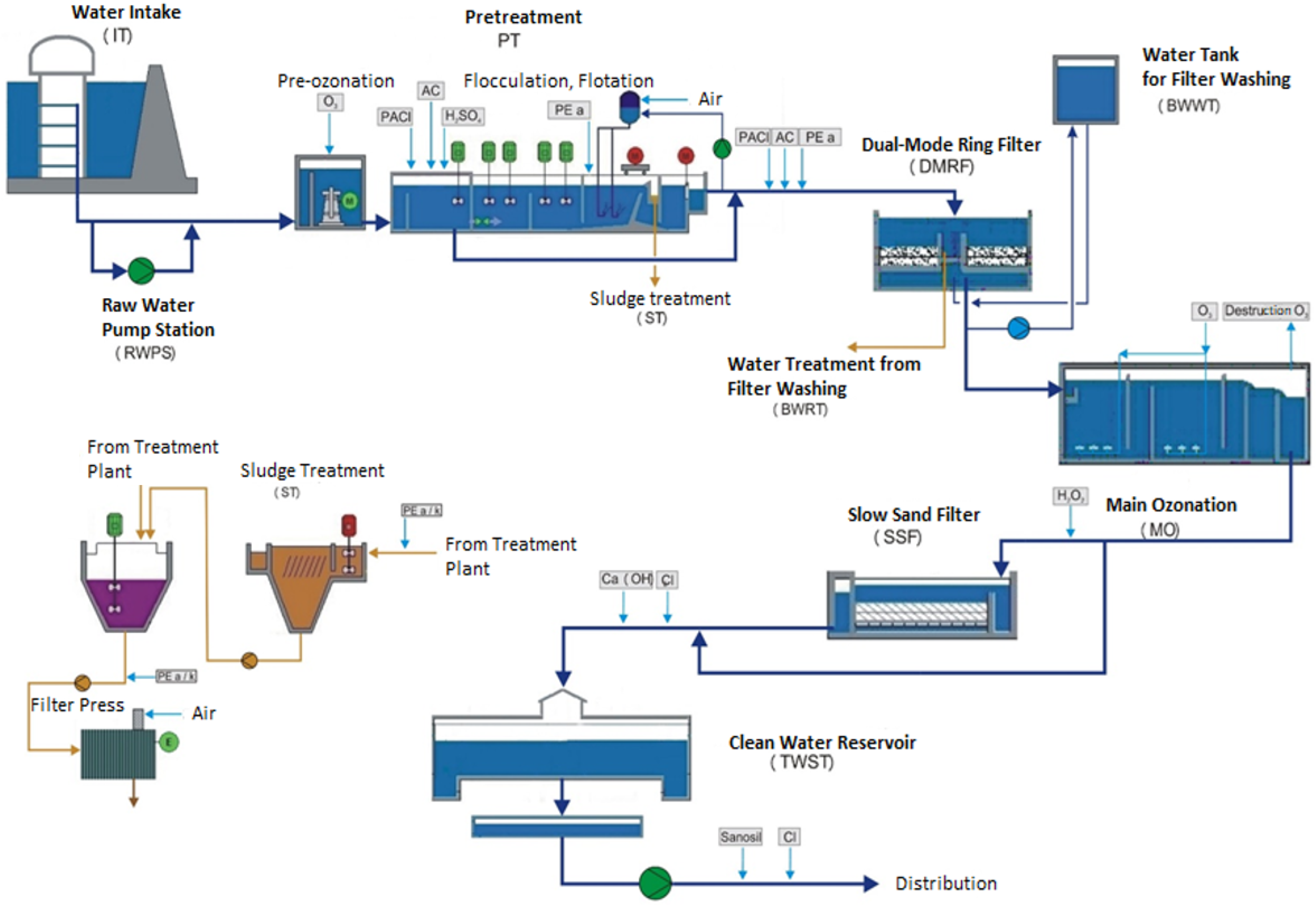
2. Study Area and Data Description

To obtain drinking water at the Butoniga DWTF, raw water is captured from the Butoniga reservoir (Figure 1). The Butoniga reservoir was created in 1987 with two primary objectives: 1. protection against adverse water impacts (floods), and 2. drinking water supply. The reservoir has a watershed area of approximately 73 km², with elevations ranging from 40 to 500 m above sea level. The reservoir has a volume of 19.5 million m³, with a surface area of approximately 2.5 km². The average depth of the reservoir is 7.8 m, and the maximum depth is 17.5 m [19].

As a small and relatively shallow reservoir, it is subjected to eutrophication and degradation processes influenced by climate change and human activities. Typical pressures in the surrounding watershed include erosion and nutrient leaching from agricultural lands, as well as untreated wastewater from nearby settlements (although in small numbers), which drains into the reservoir through black pits or open sewers. This is mainly because the sewage system is not yet completed [19].

The Butoniga DWTF is situated approximately 600 m downstream of the Butoniga reservoir dam and covers an area of 80,000 m² (Figure 1). The initial phase of the DWTF is designed to process 1000 L/s or 3600 m³/h. The treatment system is set up for a final capacity of 2000 L/s, which is planned for the second phase of the development. All process units are designed to operate at full capacity for 24 h, with a hydraulic reserve of 25%. The facility can adjust its operation flexibly, ranging from 20% to 100% of the nominal capacity [20].

Figure 1. Study area: location of the Butoniga reservoir and the drinking water treatment facility.

Figure 1. Study area: location of the Butoniga reservoir and the drinking water treatment facility.

The main drinking water treatment processes are illustrated in Figure 2 and include the following steps: raw water intake, pre-ozonation, coagulation–flocculation, flotation, rapid filtration, main ozonation, slow sand filtration, disinfection, final pH correction, pressure pumping, and chlorination. The auxiliary processes (Figure 2) include sand treatment from slow sand filters, treating the water from the rapid filter washing, sludge treatment, and neutralization of wastewater from chemical processes [20].

The facility started operating in June 2002, with continuous operation starting in the spring of 2004. The operation of the DWTF is closely linked to the tourist season. Of the 5,000,000 m³ of water produced and distributed annually, 3,000,000 m³ is produced and distributed between 15 June and 15 September, a period during which water quality in the Butoniga reservoir is at its lowest [20].

Figure 2. Schematic of the processes at the Butoniga drinking water treatment facility [14].

Figure 2. Schematic of the processes at the Butoniga drinking water treatment facility [14].

The dataset used in the modeling experiments for developing the descriptive and predictive models is presented in Table 1. The dataset consists of various physico-chemical and microbiological parameters measured once a day at the inflow of raw water from the Butoniga reservoir to the DWTF from 2011 to 2020. The time period from 2011 to 2020 was selected due to the continuity and completeness of the dataset, as it contains no gaps or missing values. Ensuring data consistency and reliability over such an extended period is crucial for building robust models and obtaining meaningful, generalizable results.

The physico-chemical parameters include water temperature (Temp), pH, water turbidity (Turbidity), oxygen concentration (O₂), total organic carbon (TOC), potassium permanganate (KMnO₄), ammonia (NH₄), manganese (Mn), aluminum (Al), iron (Fe), and the concentration of organic matter in the water (UV 254), which are determined at the internal laboratory of the Butoniga DWTF using standard analytical methods based on ISO standards, i.e., HRN EN ISO 5667-3 [21].

Among the microbiological parameters, total coliforms and E. coli bacteria are used as indicators of fecal pollution in aquatic ecosystems used for water supply, i.e., the production of potable water [3,5]. Total coliforms and E. coli bacteria were measured using the Colilert method, as specified in the standard HRN EN ISO 9308-2:2014 [22].

All the data were pre-processed in accordance with the modeling and research goals. The entire span of the measured data, collected from 2011 to 2020, was used to build the models; additionally, for the predictive models, missing data were handled using cubic spline interpolation, which uses a set of cubic polynomials between each pair of data points. Cubic spline interpolation ensures continuity of the function, as well as its first and second derivatives, resulting in a smooth and stable curve. Cubic spline interpolation is widely preferred because it produces smooth curves by ensuring continuity of the function and its first two derivatives. Unlike global polynomial methods, it offers local control; changes in one point affect only nearby segments, and it avoids unwanted oscillations. It also balances flexibility with computational efficiency and is numerically stable, even with large datasets [23].

Table 1. Physico-chemical and microbiological parameters used in the modeling experiments.

Symbol	Description	Unit
Temp	Water temperature	°C
O2	Oxygen concentration	mg/L
pH	pH	-
Tur	Water turbidity	NTU
TOC	Total organic carbon	mg/L
KMnO4	Potassium permanganate	mg/L
UV 254	Concentration of the organic matter in the water	1/cm
NH4	Ammonia	mg/L
Mn	Manganese	mg/L
Al	Aluminum	mg/L
Fe	Iron	mg/L
Tot. coliforms 1	Total coliforms	CFU/100 mL
E. coli 2	Escherichia coli	CFU/100 mL

^1,2 Total coliforms and E. coli data shifted 7 days in advance were used in the predictive models.

Table 1. Physico-chemical and microbiological parameters used in the modeling experiments.

Symbol	Description	Unit
Temp	Water temperature	°C
O2	Oxygen concentration	mg/L
pH	pH	-
Tur	Water turbidity	NTU
TOC	Total organic carbon	mg/L
KMnO4	Potassium permanganate	mg/L
UV 254	Concentration of the organic matter in the water	1/cm
NH4	Ammonia	mg/L
Mn	Manganese	mg/L
Al	Aluminum	mg/L
Fe	Iron	mg/L
Tot. coliforms 1	Total coliforms	CFU/100 mL
E. coli 2	Escherichia coli	CFU/100 mL

^1,2 Total coliforms and E. coli data shifted 7 days in advance were used in the predictive models.

3. Materials and Methods

3.1. Modeling Methods

The main modeling was performed using two different ML methods implemented within the Weka software package 3.9.6 [24]: 1. Decision trees were used for the classification of categorical outcomes, i.e., models describing and explaining total coliforms and E. coli bacteria, and 2. model trees were used for the prediction of numeric variables, i.e., models simulating/predicting total coliforms and E. coli bacteria seven days in advance. For prediction purposes, models such as RF, Multi-Layer Perceptron (M-LP), Bagging, and XGBoost were also used and comparatively evaluated in this research. All the models were implemented in the Weka software package 3.9.6, where the XGBoost model can be uploaded through a plugin package [24].

RF is an ensemble method that builds multiple DTs using different subsets of data and combines their predictions (e.g., majority voting for classification or averaging for regression). It uses random feature selection at each split, which reduces the correlation between trees and improves generalization. RF has been described as robust, accurate, and resistant to overfitting, often requiring minimal hyperparameter tuning [25].

M-LP is a type of artificial neural network (ANN) composed of at least three layers: an input layer, one or more hidden layers, and an output layer. Each neuron applies a nonlinear activation function (e.g., sigmoid, ReLU) to model complex relationships in the data. M-LP is powerful when it comes to learning nonlinear functions but can be sensitive to hyperparameters (number of hidden units, learning rate, etc.) and generally requires longer training times compared with classic methods such as trees [24].

Bagging is an ensemble technique that trains multiple models on different bootstrap samples (random sampling with replacement) of the original dataset. Its strength lies in reducing model variance, especially for decision trees, while maintaining low bias. Bagging is a common method for improving the performance of “unstable” models, making predictions more robust and less sensitive to noise [26].

Extreme Gradient Boosting (XGBoost) is an efficient implementation of the gradient boosting algorithm, which sequentially trains weak learners (usually trees) to correct the errors of previous models. It is known for high accuracy, speed, and control over overfitting through regularization. XGBoost can be considered an advanced evolution of boosting approaches, with emphasis on engineering optimization and scalability [27].

The procedure for building the DTs and MTs is provided in the text below.

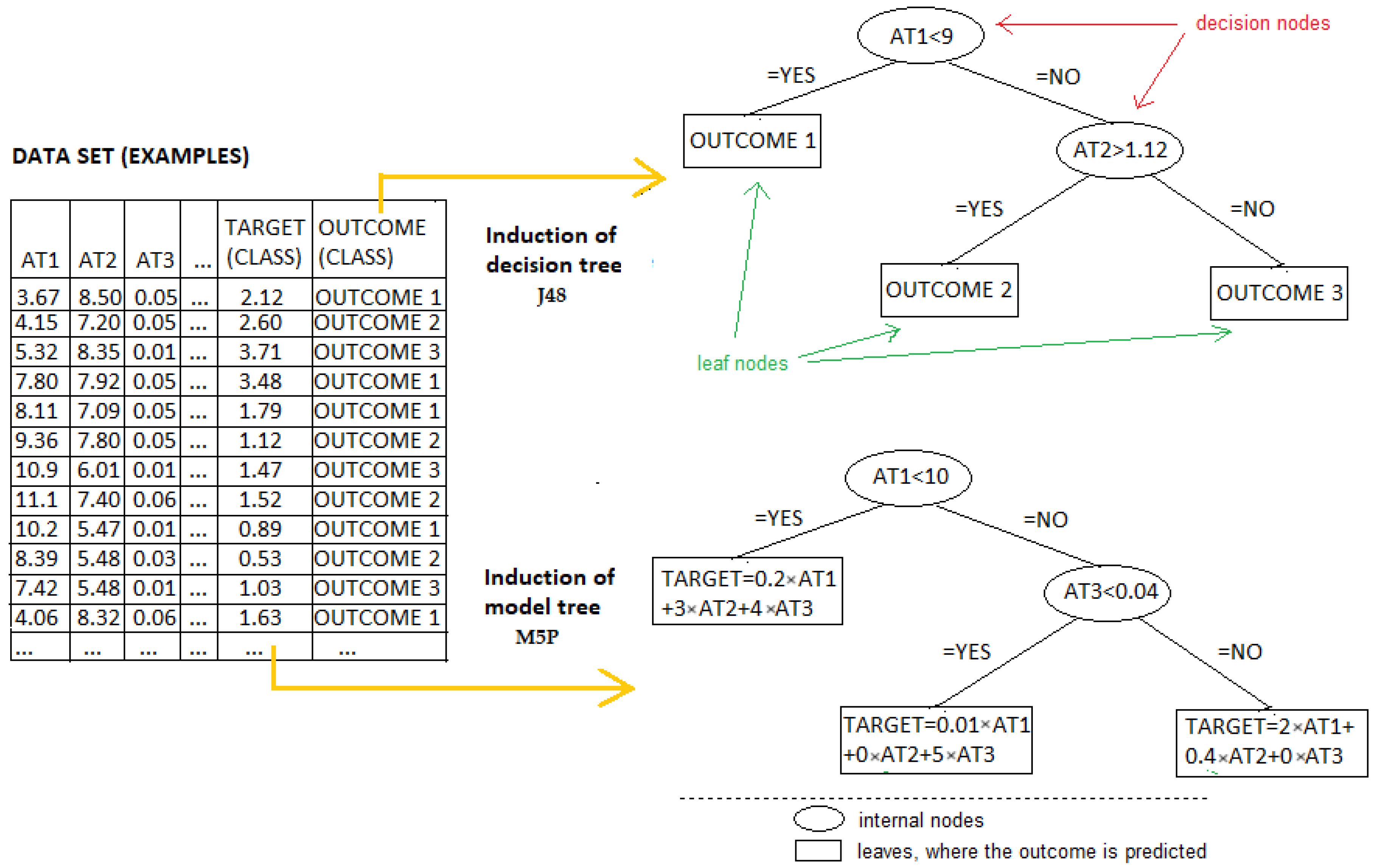
3.2. Building Decision and Model Trees

DTs are one of the concepts in ML schemes that are generated by an ML algorithm, in this case, the J48 classification based on the C4.5 algorithm [28], implemented in the Weka software package 3.9.6 [24] from given instances of that concept. Instances are characterized by the values of the attributes (independent variables) and by the outcome, which is learned by the algorithm, i.e., the class (dependent variable). The DT consists of two nodes, one called the decision node and the other the leaf node (Figure 3). Decision nodes are used to make decisions based on selected attributes and have multiple branches, whereas leaf nodes are the outcomes of those decisions and do not contain any further branches. Outcomes are presented as target (dependent) variables, while decisions or tests are performed based on the features of a given dataset [24]. DTs have more descriptive characters or capabilities, and because of this, they have been used in research to build explainable descriptive models [29].

Unlike DTs, MTs use a regression equation in the terminal leaves (Figure 3), which enables them to make a more accurate prediction of the class value; however, they are less interpretable, so this method was applied to build the predictive models. One of the most used algorithms for the induction of regression trees (RTs) and MTs is the M5 algorithm, which is based on the top-down induction of the decision tree (TDIDT) algorithm [30]. A variation of the M5 algorithm, known as M5P, was employed in the experiments conducted in this research. The algorithm was implemented in the Weka software package 3.9.6 [24,30]. Figure 3 shows the procedure for building the DTs and MTs. Like DTs, MTs also have more descriptive character or capabilities, and as a result, have been used in this research to build explainable predictive models that can be easily incorporated into future DSS development [29].

Figure 3. The procedures for building decision and model trees.

Figure 3. The procedures for building decision and model trees.

3.3. Model Evaluation and Assessment

After models have been built from the training (learning) dataset, it is necessary to assess the quality of the models, i.e., the accuracy of prediction. This can be accomplished by simulating the models on a testing dataset and comparing the predicted values of the target with the actual values. Another option is to employ the cross-validation method, where the given (training) dataset is partitioned into a chosen number of folds (n), usually 10. Each fold is used for testing, while the remaining (n−1 folds) are used for training. The final error is the average error of all the models obtained throughout the procedure [24]. The cross-validation method was used to evaluate the quality of all the models generated in the modeling experiments conducted in this study.

The size of the error between the actual and predicted values can be calculated using several measures to evaluate the model’s accuracy: root mean-squared error (RMSE), mean absolute error (MAE), root relative squared error (RRSE), relative absolute error (RAE), and the correlation coefficient (R). RMSE measures the square root of the average of the squared differences between the predicted and actual values; it gives higher weight to larger errors and is sensitive to outliers. MAE represents the average of the absolute differences between the predicted and actual values; it provides a straightforward interpretation of the average prediction error. RRSE normalizes the RMSE by the error of a simple predictor (typically the mean of the actual values), allowing for performance comparison across different datasets. RAE is similar to RRSE but is based on absolute errors; it measures the total absolute error relative to a naive baseline. The correlation coefficient (R) indicates the strength and direction of the linear relationship between the predicted and actual values; values closer to 1 or −1 imply a stronger linear relationship, while values near 0 indicate a weak or no linear correlation [24]. All these measures were used to evaluate model accuracy in the modeling experiments conducted here.

3.4. Statistical Analysis and Experimental Setup

The modeling experiments were designed to develop both descriptive and predictive models for the concentrations of total coliforms and E. coli bacteria. All the data were pre-processed in accordance with the specific objectives of the modeling task; additionally, expert knowledge from the Butoniga DWTF was incorporated into the modeling process.

For the development of the descriptive models, the J48 classification, implemented in the Weka software package [24], was used. DT models were generated to provide insight into the distribution and concentrations (classes) of total coliforms and E. coli bacteria. As mentioned, DTs are simple and easy to understand. They work well for data with categorical features and provide interpretability that other models lack. Additionally, model generation is quick, and if the pruning method is used, the models can be simple and easy to understand [29].

To ensure the reliability of the descriptive models, the input parameters in Table 1 were first subjected to attribute selection using Weka’s software package 3.9.6 built-in attribute selection algorithm [24]. For the total coliform classes, the selected attributes for building the models were pH, water temperature, water turbidity, and Mn. For the E. coli bacterial classes, the selected attributes for building the models included water turbidity, water temperature, and pH.

The corresponding histograms illustrating the distributions of the selected attributes (parameters) used for building the models based on the defined classes are presented in Figure 4 and Figure 5. The definitions of the classes are provided below.

Analysis of the histograms showing the distribution of the physico-chemical parameters across the total coliform classes (Class 0, Class 1, and Class 2) revealed notable differences between the groups (Figure 4). Temperature and pH emerged as influential factors, with Class 2 (higher concentrations) dominating at higher temperatures (above 15 °C) and elevated pH values (above 7.8), suggesting favorable conditions for the growth and survival of total coliforms. In contrast, water turbidity and Mn concentrations were generally low (but not negligible) across all the classes, including Class 2, implying that microbiological contamination can occur even at low levels of water turbidity with low metal content. The seasonal distribution showed a higher occurrence of Class 2 total coliforms in winter and early spring months, potentially linked to rainfall and/or surface runoff.

Figure 4. Histograms of selected attributes (parameters) for total coliforms.

Figure 4. Histograms of selected attributes (parameters) for total coliforms.

Figure 5. Histograms of selected attributes (parameters) for E. coli bacteria.

Figure 5. Histograms of selected attributes (parameters) for E. coli bacteria.

The distribution of the physico-chemical parameters across the E. coli classes (Class 0, Class 1, and Class 2) provides insight into the potential environmental and seasonal influences on the microbiological water quality (Figure 5). Temperature appears to play a significant role, with Class 1 (medium concentrations) and Class 2 (higher concentrations) occurring more frequently at higher temperatures (above 15 °C), which supports the hypothesis that warmer conditions favor bacterial survival and proliferation [31]. Similarly, elevated pH values (particularly above 7.8) are correlated with a higher prevalence of contaminated samples, especially in Class 1. Interestingly, turbidity does not show a strong differentiation between classes, as most samples, including those in Class 1 and Class 2, occur at low turbidity levels. The seasonal distribution highlights an increased presence of E. coli in the warmer months, particularly from May to September, which could be linked to increased rainfall, runoff, or higher biological activity.

To develop more robust and reliable models, total coliforms and E. coli bacterial concentrations were categorized into classes (Table 2), and the dataset was structured accordingly. The class definitions were established using Weka’s software package 3.9.6 clustering techniques [24], including mean values, standard deviations (STDEVs), and simple k-Means algorithms, followed by refinement based on input from expert technologists at the treatment facility (Table 2).

Table 2. Total coliform and E. coli bacterial classes defined using clustering techniques.

	Total Coliforms				E. coli Bacteria
Classes	Mean	STDEV	k-Means	Selected	Mean	STDEV	k-Means	Selected
Class 0	0–136.91	0–99.46	0–113.81	0–100	0–5.06	0–5.04	0–8.47	0–5
Class 1	136.91–417.38	99.46–356.74	113.81–476.77	100–500	5.06–47.69	5.06–44.88	8.47–57.08	5–50
Class 2	>417.38	>356.74	>476.77	>500	>47.69	>44.88	>57.08	>50

Table 2. Total coliform and E. coli bacterial classes defined using clustering techniques.

	Total Coliforms				E. coli Bacteria
Classes	Mean	STDEV	k-Means	Selected	Mean	STDEV	k-Means	Selected
Class 0	0–136.91	0–99.46	0–113.81	0–100	0–5.06	0–5.04	0–8.47	0–5
Class 1	136.91–417.38	99.46–356.74	113.81–476.77	100–500	5.06–47.69	5.06–44.88	8.47–57.08	5–50
Class 2	>417.38	>356.74	>476.77	>500	>47.69	>44.88	>57.08	>50

During model construction, the total coliform and E. coli bacterial classes were set as the target (dependent) variables, whereas water temperature, pH, water turbidity, and Mn (attributes selected by Weka’s software package 3.9.6 built-in attribute selection algorithm [15]), as listed in Table 1, were treated as the independent variables (descriptors) used to model the defined classes.

A basic statistical analysis overview, along with the chosen class boundaries for total coliforms and E. coli, is illustrated in Figure 6 and Figure 7, respectively.

Figure 6 summarizes the average monthly variation in the total coliform concentrations in the raw water at the DWTF over a ten-year period (2011–2020). The summary statistics include minimum (MIN), maximum (MAX), standard deviation (STDEV), and average values for each month, providing insight into long-term seasonal dynamics. The monthly average concentrations ranged from 230 to 477, with the lowest values observed in the winter months (e.g., January and February) and the highest values typically occurring during the summer and early autumn (e.g., July and September). This pattern suggests a clear seasonal trend, with elevated total coliform levels during the warmer months likely influenced by higher temperatures and increased biological activity [31]. The maximum concentrations peaked at 991 CFU/100 mL, with the extreme values also concentrated in the summer and early autumn period. In contrast, the minimum values ranged between 26 and 248 CFU/100 mL, generally corresponding to the colder months. The standard deviation values, which ranged from 149 to 340, indicated considerable intra-month variability over the years. Higher standard deviations were typically associated with months exhibiting both high maximum values and elevated averages, reflecting the episodic nature of contamination events, likely driven by variable hydro-meteorological and land-use conditions. Overall, the data reveal a recurring seasonal pattern for total coliform levels.

Figure 6. Basic statistical analysis and chosen class limits for total coliforms.

Figure 6. Basic statistical analysis and chosen class limits for total coliforms.

Figure 7 illustrates the average monthly E. coli concentrations in the raw water at the DWTF over a ten-year period (2011–2020). The descriptive statistics include MIN, MAX, STDEV, and average values (AVERAGE), highlighting long-term seasonal and inter-annual trends in the microbial water quality. The average E. coli concentrations show clear temporal variability, ranging from as low as 3 CFU/100 mL (April) to peaks of 55 CFU/100 mL (August). The lowest monthly averages were consistently observed during late winter and early spring (February to April), while the highest values were recorded in the summer and early autumn months (August to October). This seasonal pattern aligns with warmer temperatures, which are known to influence fecal contamination levels in surface water bodies [31]. The monthly maximum concentrations varied substantially, reaching up to 195 CFU/100 mL in December, indicating sporadic contamination events even during the colder months. In contrast, the minimum values were close to zero for several months, confirming low baseline levels during periods of reduced microbial activity or favorable hydrological conditions. The standard deviation values ranged from 2 to 58, with higher values in the second half of the year, particularly in late summer and autumn, suggesting greater temporal fluctuations and potential short-term spikes in contamination. This variability may be linked to recreational activities or agricultural practices in the watershed area [20]. These findings underscore the importance of dynamic and seasonal monitoring strategies for E. coli, especially in the summer months when levels are more likely to exceed regulatory thresholds.

Total coliforms act as a broad indicator of environmental contamination, influenced by various physico-chemical and seasonal factors; in contrast, E. coli serves as a more targeted indicator of recent fecal contamination and exhibits a stronger association with elevated temperatures and summer months. These complementary patterns underscore the importance of using both indicators for comprehensive microbial water quality assessment [3,4].

Figure 7. Basic statistical analysis and chosen class limits for E. coli bacteria.

Figure 7. Basic statistical analysis and chosen class limits for E. coli bacteria.

Predictive models were developed using the M5P algorithm for MT induction, as implemented in the Weka software package 3.9.6 [24]. The training dataset was structured so that the concentrations of total coliforms and E. coli bacteria, predicted seven days in advance, served as the target variables. The independent variables included all relevant parameters necessary for building accurate models: water temperature, pH, water turbidity, KMnO₄, NH₄⁺, Mn, Al, Fe, O₂, TOC, UV 254, and the current concentrations of total coliforms and E. coli bacteria (Table 1). MTs are simple and easy to understand, and they can be easily (when pruned) incorporated into MS Excel. They work well and provide interpretability that other models lack. Additionally, model generation is quick, and if pruning is used, the generated models can be simple and easy to understand [29]. As a result, such models can support a DSS and inform timely decision-making during water treatment operations, contributing to more resilient and proactive management of raw water quality. RF, M-LP, Bagging, and XGBoost predictive models were also developed and comparatively evaluated according to the above guidelines.

In consultation with the facility’s chief technologist, a seven-day prediction window was selected to provide sufficient time for intervention and appropriate operational responses in the event of elevated total coliform or E. coli bacterial concentrations in the raw water.

The selected parameters accurately reflect the main characteristics of the analyzed system, namely, the Butoniga reservoir and the DWTF on which the target variables rely.

The cross-validation method was used to assess the quality of the obtained models, where the given dataset (for training the model) is divided into a selected number of parts (n), in this case 10, and each part is then used for testing, while the rest (n-1 parts) are used for training the model. The final error is the average error of all the models obtained during the entire procedure [24].

To assess model accuracy, the size of the error between the actual and simulated (predicted) values was calculated using several methods: RMSE, MAE, RRSE, RAE, and R [24].

4. Results and Discussion

The models were developed to describe, i.e., explain and predict, microbiological activity and dynamics, specifically, the concentrations of total coliforms and E. coli bacteria up to seven days in advance. The primary objective of the generated models was to support and improve the optimization of water treatment processes and enhance the long-term sustainability of the DWTF as part of the DSS by enabling timely responses to fluctuations in the quality of the raw water originating from the Butoniga reservoir. Accordingly, the resulting models provide a valuable decision support tool for managing treatment operations that are highly sensitive to variations in source water conditions.

4.1. Descriptive Models

Descriptive models in the form of DTs were developed for the microbiological indicators, specifically the classes of total coliforms and E. coli bacteria outlined in Section 3.4. When constructing the models, the respective bacterial classes (as defined in Table 2) were used as the target (dependent) variables, while water temperature, pH, water turbidity, and Mn (Table 1) served as the independent variables (descriptors) to model the defined classes. These variables acted as descriptors for modeling the total coliform and E. coli bacterial classes.

The resulting DT models for total coliform and E. coli bacterial classes are presented in Figure 8 and Figure 9, respectively. Although the models exhibit a relatively low correlation, they provide a meaningful representation of the dynamics of the total coliforms and E. coli bacteria in the water intended for treatment at the DWTF, particularly considering the complexity of the problem domain.

4.1.1. Descriptive Model for Total Coliforms

The model for total coliforms is presented in Figure 8, showing a classification accuracy exceeding 60%. Additional model performance metrics include an MAE of 0.346, an RMSE of 0.413, an RAE of 88.14%, and an RRSE of 92.46%.

As illustrated in Figure 8, pH emerges as the most influential parameter in the classification of total coliforms. According to the model, higher concentrations of total coliforms (Class 2) are primarily associated with lower pH values (pH < 8.1), higher water turbidity levels (Turbidity > 8.83), and elevated water temperatures (Temp > 15.5), as observed on the left side of the decision tree. pH is a critical factor influencing both the growth and survival of bacteria in aquatic environments [32]. Elevated water turbidity is commonly associated with microbiological contamination, including total coliforms, as previously reported in [8]. Water turbidity also reflects the presence of suspended particles in the water column and is influenced by various sources of organic material, including algae, colloids, decaying matter, and sediment [31]. Water temperature also plays a key role in microbial dynamics; higher temperatures tend to accelerate bacterial growth, while lower temperatures inhibit it [31].

Lower concentrations of total coliforms (Class 0) are associated with higher pH levels (pH > 8.1), lower water temperatures (Temp < 11.1), and elevated Mn concentrations (Mn > 0.092), as seen on the right side of the decision tree, an outcome consistent with the explanations provided above. On the left side of the tree, Class 0 is linked to lower pH values (pH < 8.1) but only in combination with low water turbidity (Turbidity < 8.83 and <1.85) and lower water temperatures (Temp < 15.5 °C). Mn, along with iron (Fe) and ammonium (NH₄), represents a key parameter for water quality in the Butoniga reservoir. During the summer months, increased concentrations of Mn, Fe, and NH₄ in the raw water, especially under lower pH conditions when the water is captured from the lowest water intake, require enhanced process control and greater chemical consumption during treatment at the DWTF [20]. Mn may also influence microbiological water quality, as higher Mn concentrations are often associated with increased levels of total coliforms [33].

Class 1 of total coliforms, which represents concentrations between the lowest and highest concentrations, is associated with a combination of parameters like pH, water turbidity, water temperature, and Mn, all of which influence total coliform levels.

Figure 8. Descriptive model for concentrations of total coliforms in water captured from the Butoniga reservoir during the study period from 2011 to 2020.

Figure 8. Descriptive model for concentrations of total coliforms in water captured from the Butoniga reservoir during the study period from 2011 to 2020.

4.1.2. Descriptive Model for E. coli Bacteria

The DT model for E. coli bacteria, presented in Figure 9, achieved a classification accuracy of over 70%. The model’s performance was further evaluated using standard regression metrics, yielding an MAE of 0.304, an RMSE of 0.3885, an RAE of 76.64%, and an RRSE of 87.19%.

As indicated in Figure 9, water turbidity was identified as the most significant predictor of E. coli bacterial class assignment. Higher concentrations of E. coli (Class 2) were associated with elevated water turbidity levels (Turbidity > 3.4 and >7.46) and pH values between 7.5 and 8.1. Increased water turbidity is commonly associated with microbiological contamination, including E. coli bacteria, as previously reported [8]. In addition, the study [34] demonstrated strong correlations between E. coli levels and pH (R² = 0.84), water turbidity (R² = 0.83), and total dissolved solids (TDSs, R² = 0.70). The pH is also a critical factor in evaluating water system toxicity, as local fluctuations are often associated with microbiological activity and the growth of potentially harmful organisms [9].

Lower E. coli bacterial concentrations (Class 0) were predominantly observed under conditions of reduced water turbidity (Turbidity ≤ 3.4) and lower water temperatures (Temp ≤ 16.1), which aligns with the findings reported above. As previously noted, water temperature is a key environmental variable influencing the growth of microorganisms, with lower water temperatures slowing their growth [31].

Class 1, representing intermediate E. coli bacterial levels, corresponded to more variable combinations of water turbidity, pH, and water temperature, indicating more complex interactions among these parameters.

Figure 9. Descriptive model for E. coli bacterial concentrations in water captured from the Butoniga reservoir for the study period from 2011 to 2020.

Figure 9. Descriptive model for E. coli bacterial concentrations in water captured from the Butoniga reservoir for the study period from 2011 to 2020.

4.2. Predictive Models

To build the predictive models, the MT, RF, M-LP, Bagging, and XGBoost methods were employed, and MT was chosen for final consideration (Table 3). In these models, the concentrations of total coliforms and E. coli bacteria, shifted seven days ahead, were used as target (dependent) variables. The independent variables included water temperature, pH, water turbidity, KMnO₄, NH₄, Mn, Al, Fe, O₂, TOC, UV 254, and the current concentrations of total coliforms and E. coli bacteria (Table 1).

The resulting predictive models generated using MTs are presented in Figure 10 and Figure 11, with the corresponding model equations detailed in Table 4 and Table 5. Although the models do not yield high correlation coefficients, they provide acceptable predictive performance for describing the dynamics of total coliforms and E. coli bacteria, particularly in light of the inherent complexity of the domain.

Importantly, such models can support the DSS and inform timely decision-making during water treatment operations, contributing to more resilient and proactive management of raw water quality.

RF, M-LP, Bagging, and XGBoost models were also developed and comparatively evaluated as part of this modeling experiment (Table 3). The quality of the models, i.e., the accuracy of prediction, was determined by employing a 10-fold cross-validation method [24]. The size of the error between the actual and predicted values was measured using RMSE, MAE, RRSE, RAE, and R to evaluate model accuracy.

Table 3. Accuracies of the developed predictive models based on standard regression accuracy metrics.

	Total Coliforms					E. coli Bacteria
Measures	Model Trees	RF	M-LP	Bagging	XGBoost	Model Trees	RF	M-LP	Bagging	XGBoost
R	0.72	0.80	0.45	0.73	0.89	0.48	0.60	0.42	0.55	0.78
MAE	205.28	138.79	273.17	165.94	111.82	26.5	17.41	28.87	20.13	15.11
RMSE	267.32	203.19	350.37	230.66	185.06	57.7	50.10	58.96	51.89	46.62
RAE (%)	70.06	48.70	95.84	58.22	44.56	69.3	55.89	92.70	64.63	49.62
RRSE (%)	78.8	59.94	103.37	68.05	53.47	73.8	80.30	94.51	83.19	75.23

Table 3. Accuracies of the developed predictive models based on standard regression accuracy metrics.

	Total Coliforms					E. coli Bacteria
Measures	Model Trees	RF	M-LP	Bagging	XGBoost	Model Trees	RF	M-LP	Bagging	XGBoost
R	0.72	0.80	0.45	0.73	0.89	0.48	0.60	0.42	0.55	0.78
MAE	205.28	138.79	273.17	165.94	111.82	26.5	17.41	28.87	20.13	15.11
RMSE	267.32	203.19	350.37	230.66	185.06	57.7	50.10	58.96	51.89	46.62
RAE (%)	70.06	48.70	95.84	58.22	44.56	69.3	55.89	92.70	64.63	49.62
RRSE (%)	78.8	59.94	103.37	68.05	53.47	73.8	80.30	94.51	83.19	75.23

As shown in Table 3, a comparison of the MT, RF, M-LP, Bagging, and XGBoost predictive models was performed using standard regression accuracy metrics: R, MAE, RMSE, RAE, and RRSE.

The results show that XGBoost and RF achieved the best performance for both target variables; specifically, for total coliforms, XGBoost gave the highest R value (0.89) and the lowest error values (MAE = 111.82, RMSE = 185.06), while RF also demonstrated competitive results. Similarly, for E. coli, XGBoost gave the best results (R = 0.78, MAE = 15.11, RMSE = 46.62).

On the other hand, the M-LP model showed the weakest performance, with the lowest R values and the highest error metrics, indicating limited suitability for the given dataset.

In [16], the RF algorithm outperformed an ANN in over 90% of the trained binary classification models. Based on the results reported in [18], the XGBoost model achieved superior estimation accuracy and offered better explanations of the variable contributions compared with the RF, DNN, and CNN models. In [11], although RF, Gradient Boosting, and Extremely Randomized Trees (ERTs) produced consistent classification results, the highest testing accuracies were achieved using DTs with Adaptive Boosting and Bagging techniques.

Overall, despite the superior accuracy of the XGBoost model, the MT was selected as the final model due to its simplicity, interpretability, and transparency, aspects that are particularly important in the context of microbiological water quality management and data-driven decision-making. The trade-off between accuracy and interpretability makes MTs (in this case) a suitable choice for operational implementation as part of a DSS at the Butoniga DWTF [11].

The results of the predictive models using MTs for total coliforms and E. coli bacteria are provided in the following subsections.

4.2.1. Predictive Model for Total Coliforms

The predictive model for total coliforms is presented in Figure 10, with the corresponding regression equations provided in Table 4. The model consists of ten terminal nodes (leaves), each associated with a specific equation used to estimate total coliform concentrations seven days in advance, based on the input variables defined in the internal nodes of the MT (Figure 10).

Analysis of the model structure indicates that the most influential predictors include the current concentration of total coliforms (as anticipated), along with NH₄ levels, pH values, water temperature, UV 254 absorbance, and TOC. Table 4 provides the equations corresponding to each leaf of the model tree, which incorporate various combinations of these parameters, such as water temperature, O₂, pH, TOC, UV 254, NH₄, and the current total coliform levels.

The model operates by selecting the appropriate leaf based on the values of the variables at each decision node. Once a specific path is followed through the tree, the associated linear equation is applied to predict total coliform concentrations seven days ahead.

While the model provides a reasonable approximation of microbiological prediction dynamics under varying water quality conditions, its predictive reliability may be influenced by local environmental variability and unmeasured external factors not captured in the dataset.

Figure 10. Predictive model for total coliforms 7 days in advance in water captured from the Butoniga reservoir.

Figure 10. Predictive model for total coliforms 7 days in advance in water captured from the Butoniga reservoir.

Table 4. Equations for the model tree presented in Figure 10 (total coliforms prediction).

Equation No.	Equation
1.	Tot. coliforms pred = 0.1099 × Temp − 12.6543 × pH − 1.514 × TOC + 20.0651 × UV 254 − 14.1254 × NH4 + 0.0189 × Tot. coliforms + 286.8738
2.	Tot. coliforms pred = 0.1099 × Temp − 14.835 × pH − 1.514 × TOC + 20.0651 × UV 254 − 5.2055 × NH4 + 0.0189 × Tot. coliforms + 262.9118
3.	Tot. coliforms pred = 0.1099 × Temp − 12.0872 × pH − 1.514 × TOC + 20.0651 × UV 254 − 5.2055 × NH4 + 0.0189 × Tot. coliforms + 175.9947
4.	Tot. coliforms pred = 0.351 × Temp − 0.8502 × pH − 4.4381 × TOC + 78.196 × UV 254 − 0.551 × NH4 + 0.0125 × Tot. coliforms + 226.4315
5.	Tot. coliforms pred = 0.1619 × Temp − 0.8502 × pH − 5.5019 × TOC + 160.9756 × UV 254 − 0.551 × NH4 + 0.0125 × Tot. coliforms + 246.5877
6.	Tot. coliforms pred = 0.1619 × Temp − 0.8502 × pH − 5.9023 × TOC + 90.2781 × UV 254 − 0.551 × NH4 + 0.0125 × Tot. coliforms + 373.1973
7.	Tot. coliforms pred = 0.1619 × Temp − 0.8502 × pH − 11.999 × TOC + 90.2781 × UV 254 − 0.551 × NH4 + 0.0125 × Tot. coliforms + 288.8409
8.	Tot. coliforms pred = − 0.0978 × Temp − 0.4027 × pH − 0.4387 × TOC + 7.7413 × UV 254 + 0.0143 × Tot. coliforms + 532.73
9.	Tot. coliforms pred = − 0.1405 × Temp − 0.4027 × pH − 0.4387 × TOC + 7.7413 × UV 254 + 0.0143 × Tot. coliforms + 23.2427
10.	Tot. coliforms pred = 0.0508 × Temp − 0.4027 × pH − 0.4387 × TOC + 7.7413 × UV 254 + 0.0189 × Tot. coliforms + 727.1597

Table 4. Equations for the model tree presented in Figure 10 (total coliforms prediction).

Equation No.	Equation
1.	Tot. coliforms pred = 0.1099 × Temp − 12.6543 × pH − 1.514 × TOC + 20.0651 × UV 254 − 14.1254 × NH4 + 0.0189 × Tot. coliforms + 286.8738
2.	Tot. coliforms pred = 0.1099 × Temp − 14.835 × pH − 1.514 × TOC + 20.0651 × UV 254 − 5.2055 × NH4 + 0.0189 × Tot. coliforms + 262.9118
3.	Tot. coliforms pred = 0.1099 × Temp − 12.0872 × pH − 1.514 × TOC + 20.0651 × UV 254 − 5.2055 × NH4 + 0.0189 × Tot. coliforms + 175.9947
4.	Tot. coliforms pred = 0.351 × Temp − 0.8502 × pH − 4.4381 × TOC + 78.196 × UV 254 − 0.551 × NH4 + 0.0125 × Tot. coliforms + 226.4315
5.	Tot. coliforms pred = 0.1619 × Temp − 0.8502 × pH − 5.5019 × TOC + 160.9756 × UV 254 − 0.551 × NH4 + 0.0125 × Tot. coliforms + 246.5877
6.	Tot. coliforms pred = 0.1619 × Temp − 0.8502 × pH − 5.9023 × TOC + 90.2781 × UV 254 − 0.551 × NH4 + 0.0125 × Tot. coliforms + 373.1973
7.	Tot. coliforms pred = 0.1619 × Temp − 0.8502 × pH − 11.999 × TOC + 90.2781 × UV 254 − 0.551 × NH4 + 0.0125 × Tot. coliforms + 288.8409
8.	Tot. coliforms pred = − 0.0978 × Temp − 0.4027 × pH − 0.4387 × TOC + 7.7413 × UV 254 + 0.0143 × Tot. coliforms + 532.73
9.	Tot. coliforms pred = − 0.1405 × Temp − 0.4027 × pH − 0.4387 × TOC + 7.7413 × UV 254 + 0.0143 × Tot. coliforms + 23.2427
10.	Tot. coliforms pred = 0.0508 × Temp − 0.4027 × pH − 0.4387 × TOC + 7.7413 × UV 254 + 0.0189 × Tot. coliforms + 727.1597

The model presented in Figure 10 and Table 4 achieved a correlation coefficient of 0.72, indicating a strong linear relationship between the predicted and observed values. Additional performance metrics include an MAE of 205.28, an RMSE of 267.32, an RAE of 70.06%, and an RRSE of 78.8%. The predictive performance of the model is illustrated in Figure 11.

As shown in Figure 11, the model performs well in estimating total coliform concentrations up to approximately 750 CFU/100 mL; however, it tends to under-predict higher values. This underestimation may be attributed to the lower frequency of and higher variability in extreme values, which increases the difficulty of accurately capturing them through regression-based methods.

An error analysis was conducted specifically for all the extreme cases within the dataset where the prediction performance significantly decreased, particularly for samples with total coliform concentrations above 750 CFU/100 mL. These cases are especially important from a microbiological and public health perspective and require special attention during model evaluation. For these extreme cases, the model yielded an MAE of 398.12 and an RMSE of 437.13, indicating substantial deviations between the predicted and actual values; in contrast, the overall dataset (including all values) resulted in an MAE of 205.28 and an RMSE of 26.327. This comparison suggests that the model struggles to maintain accuracy when dealing with high total coliform concentrations, with error levels nearly doubling in extreme cases. Identifying these limitations is crucial for guiding future model improvements and potentially developing targeted sub-models or correction strategies focused on high-risk events.

Furthermore, the structure of the model (Figure 10, Table 4) confirms that the parameters selected in the MT play a significant role in influencing total coliform concentrations, consistent with the findings discussed in Section 4.1.1 [31,32,33].

Figure 11. Comparison of measured (shifted) versus predicted values obtained by the model for total coliforms during the modeled period.

Figure 11. Comparison of measured (shifted) versus predicted values obtained by the model for total coliforms during the modeled period.

4.2.2. Predictive Model for E. coli Bacteria

The predictive model for E. coli bacterial concentrations is illustrated in Figure 12, with the corresponding regression equations detailed in Table 5. This model consists of ten terminal nodes (leaves), each associated with a specific equation used to predict the E. coli concentrations seven days in advance based on the input variables defined at the internal nodes of the MT (Figure 12).

An analysis of the MT structure identifies the most influential predictors as the current concentration of E. coli (as anticipated), pH values, and O₂ levels, followed by the NH₄, Fe, and KMnO₄ concentrations, along with water turbidity. Table 5 provides the equations associated with each leaf, which incorporate various combinations of these parameters together with the current E. coli concentration.

The model operates by navigating through the decision nodes based on the values of these variables; once the appropriate leaf is reached, the corresponding equation is applied to predict E. coli concentrations seven days ahead.

Figure 12. Predictive model for E. coli bacteria 7 days in advance in water captured from the Butoniga reservoir.

Figure 12. Predictive model for E. coli bacteria 7 days in advance in water captured from the Butoniga reservoir.

Table 5. Equations for the model tree presented in Figure 8 (E. coli bacteria prediction).

Equation No.	Equation
1.	E. coli pred = − 0.0094 × O2 − 1.0048 × pH + 0.0719 × KMnO4 − 0.302 × NH4 + 0.6454 × Fe + 0.0017 × E. coli + 27.4774
2.	E. coli pred = − 0.0094 × O2 − 1.7702 × pH + 0.0719 × KMnO4 − 0.6939 × NH4 + 0.6454 × Fe + 0.0017 × E. coli + 23.4384
3.	E. coli pred = − 0.0094 × O2 − 1.4932 × pH + 0.0719 × KMnO4 − 0.3272 × NH4 + 0.6454 × Fe + 0.0017 × E. coli + 19.8177
4.	E. coli pred = − 0.0094 × O2 − 1.5966 × pH + 0.0719 × KMnO4 − 0.3272 × NH4 + 0.6454 × Fe + 0.0017 × E. coli + 17.6368
5.	E. coli pred = − 0.0445 × O2 − 0.4569 × pH + 0.2575 × Turbidity − 0.1558 × KMnO4 + 1.4384 × Fe + 0.0014 × E. coli + 47.3177
6.	E. coli pred = − 0.0445 × O2 − 0.4569 × pH + 0.2575 × Turbidity − 0.1558 × KMnO4 + 1.4384 × Fe + 0.0014 × E. coli + 35.5702
7.	E. coli pred = − 0.0445 × O2 − 0.4569 × pH + 0.6061 × Turbidity − 0.744 × KMnO4 + 1.4384 × Fe + 0.0014 × E. coli + 90.2576
8.	E. coli pred = − 0.0445 × O2 − 0.4569 × pH + 0.3106 × Turbidity + 0.0609 × KMnO4 + 1.4384 × Fe + 0.0014 × E. coli + 69.5288
9.	E. coli pred = − 0.0525 × O2 − 0.5132 × pH + 0.0291 × Turbidity + 0.0609 × KMnO4 + 3.8009 × Fe + 0.0014 × E. coli + 20.6872
10.	E. coli pred = − 0.0525 × O2 − 0.5132 × pH + 0.0291 × Turbidity + 0.0609 × KMnO4 + 3.3453 × Fe + 0.0014 × E. coli + 39.9425

Table 5. Equations for the model tree presented in Figure 8 (E. coli bacteria prediction).

Equation No.	Equation
1.	E. coli pred = − 0.0094 × O2 − 1.0048 × pH + 0.0719 × KMnO4 − 0.302 × NH4 + 0.6454 × Fe + 0.0017 × E. coli + 27.4774
2.	E. coli pred = − 0.0094 × O2 − 1.7702 × pH + 0.0719 × KMnO4 − 0.6939 × NH4 + 0.6454 × Fe + 0.0017 × E. coli + 23.4384
3.	E. coli pred = − 0.0094 × O2 − 1.4932 × pH + 0.0719 × KMnO4 − 0.3272 × NH4 + 0.6454 × Fe + 0.0017 × E. coli + 19.8177
4.	E. coli pred = − 0.0094 × O2 − 1.5966 × pH + 0.0719 × KMnO4 − 0.3272 × NH4 + 0.6454 × Fe + 0.0017 × E. coli + 17.6368
5.	E. coli pred = − 0.0445 × O2 − 0.4569 × pH + 0.2575 × Turbidity − 0.1558 × KMnO4 + 1.4384 × Fe + 0.0014 × E. coli + 47.3177
6.	E. coli pred = − 0.0445 × O2 − 0.4569 × pH + 0.2575 × Turbidity − 0.1558 × KMnO4 + 1.4384 × Fe + 0.0014 × E. coli + 35.5702
7.	E. coli pred = − 0.0445 × O2 − 0.4569 × pH + 0.6061 × Turbidity − 0.744 × KMnO4 + 1.4384 × Fe + 0.0014 × E. coli + 90.2576
8.	E. coli pred = − 0.0445 × O2 − 0.4569 × pH + 0.3106 × Turbidity + 0.0609 × KMnO4 + 1.4384 × Fe + 0.0014 × E. coli + 69.5288
9.	E. coli pred = − 0.0525 × O2 − 0.5132 × pH + 0.0291 × Turbidity + 0.0609 × KMnO4 + 3.8009 × Fe + 0.0014 × E. coli + 20.6872
10.	E. coli pred = − 0.0525 × O2 − 0.5132 × pH + 0.0291 × Turbidity + 0.0609 × KMnO4 + 3.3453 × Fe + 0.0014 × E. coli + 39.9425

The model presented in Figure 12 and Table 5 exhibits a moderate correlation coefficient of 0.48. Additional performance metrics include an MAE of 26.5, an RMSE of 57.7, an RAE of 69.3%, and an RRSE of 73.8%. The prediction performance is illustrated in Figure 13.

As observed in Figure 13, the relatively low correlation coefficient is largely attributable to the model’s limited ability to accurately predict peak E. coli concentrations. While the model reliably estimates concentrations up to approximately 100 CFU/100 mL, it tends to underestimate higher values. This under-prediction likely arises from the scarcity of and high variability in extreme observations, which pose challenges for regression-based approaches.

An error analysis was also conducted for the E. coli predictions, focusing on all the extreme cases within the dataset (E. coli > 100 CFU/100 mL). The results revealed a substantial decrease in prediction accuracy in these high-concentration instances. For the extreme E. coli values, the model produced an MAE of 844.55 and an RMSE of 848.84. These values are significantly higher than the error metrics calculated across the entire dataset, where the MAE was 26.5 and the RMSE was 57.5. This sharp increase in both MAE and RMSE indicates that the model struggles to generalize well when handling unusually high E. coli concentrations. Such results underline the need for enhanced model robustness or possibly the introduction of threshold-specific calibration strategies. Recognizing and quantifying these error patterns helps improve risk-based decision-making and supports the future development of more resilient prediction frameworks.

Furthermore, the structure of the model (Figure 12, Table 5) confirms that the variables incorporated in the model tree significantly influence E. coli concentrations, as discussed in Section 4.1.2 [8,9,31,34].

Figure 13. Comparison of measured (shifted) versus predicted values obtained by the model of E. coli bacteria for the modeled period.

Figure 13. Comparison of measured (shifted) versus predicted values obtained by the model of E. coli bacteria for the modeled period.

4.3. Final Discussion and Remarks

Regardless of the inherent challenges, models predicting total coliforms and E. coli bacterial concentrations seven days in advance can significantly aid in managing specific drinking water treatment processes, depending on the biological quality of the raw water from the Butoniga reservoir. While predicting microbiological parameters is inherently complex and no model can be expected to perfectly reproduce all peak values, discrepancies between measured and predicted concentrations can provide valuable operational insights. Such deviations may indicate potential issues requiring attention, such as failures in wastewater infrastructure or diffuse contamination sources [8].

The models developed in this research were constructed using ML methods implemented in the Weka software package [24]. ML methods such as DT, MT, RF, M-LP, Bagging, and XGBoost were used to build descriptive and predictive models and were comparatively evaluated. Despite the superior accuracy of the XGBoost model, DTs and MTs, which fall under the category of “transparent-box” models, were chosen for further use. DTs and MTs are advantageous due to their simplicity, interpretability, and transparency, attributes that are particularly important in microbiological water quality management and data-driven decision-making [35]. These characteristics make DTs and MTs more understandable compared with more complex “black-box” models. As such, DT and MT were selected for further application and integration into the future development of a DSS.

The trade-off between predictive accuracy and model interpretability makes both DT and MT models particularly suitable for operational implementation into the DSS at the Butoniga DWTF.

Despite the satisfactory performance of the MT model compared with the other models (Table 3) in predicting total coliform and E. coli bacterial concentrations, the model exhibits limited accuracy in forecasting extreme values. This limitation is primarily attributed to the low frequency of and high variability in peak concentrations within the dataset, which constrains the model’s generalizability beyond typical conditions [36,37]. Although the error analysis for extreme concentrations (above typical operational ranges) showed higher values, this is not considered critical in the context of model application. Peak values are not the primary focus of routine operational decision-making. The model performs well within the regular range of concentrations, where most real-time decisions are made; therefore, while the errors for extreme cases are higher, they do not significantly affect the practical usability of the model for supporting day-to-day microbiological water quality assessments. More complex ML approaches such as RF, SVM, kNN, ANN, GBR, Bagging, Boosting, and XGBoost may improve prediction accuracy but are sometimes less practical for direct implementation in routine operational environments due to their complexity and need for specialized expertise [11,12,16,17,18,38,39].

Additionally, incorporating external environmental variables, such as rainfall, reservoir inflow, and other hydrological or meteorological factors, may enhance the robustness and reliability of predictions under highly dynamic water quality conditions [38,39].

Currently, the adoption of ML techniques is steadily increasing across various aspects of DWTF modeling, including prediction, optimization, and facility management. For instance, Khan et al. [9] employed a superposition learning-based model to predict E. coli levels in groundwater using physico-chemical water quality parameters. Their results indicated that the model, which included inputs such as turbidity, pH, total dissolved solids (TDSs), and electrical conductivity (EC), achieved the best performance with an R value of 0.90 and a lowest mean squared error (MSE) of 0.0892. Stocker et al. [6] predicted E. coli concentrations in agricultural pond waters using several ML methods: SGB machines and the RF, SVM, and kNN algorithms. The RF algorithm offered better predictions in more cases than the other models when assessed in terms of the average values of RMSE, coefficient of determination, and MAE; nevertheless, when the performance metrics were treated as statistics, there was no significant difference between the performance of the ML algorithms in most cases. Similarly, Sokolova et al. [8] focused on predicting microbial water quality in drinking water sources by monitoring E. coli and utilizing hydro-meteorological data with data-driven models. Their study revealed that models incorporating multiple predictors, such as VAR, LASSO Regression, RF, and TPOT, performed better than univariate models, such as the naive baseline, exponential smoothing, and ARIMA. For example, the coefficient of determination (R²) for the test data was 0.35 for ARIMA, 0.56 for VAR, 0.51 for LASSO, 0.46 for RF, and 0.60 for TPOT. Additionally, the inclusion of external predictors enhanced model performance, suggesting that some of these models are effective for forecasting E. coli concentrations at water intakes. Mohammed et al. [40] presented comparative predictive modeling of the occurrence of fecal indicator bacteria in a drinking water source in Norway. For prediction modeling of coliform bacteria, E. coli, intestinal enterococci, and Clostridium perfringens, Mohammed et al. [40] used zero-inflated (ZI) regression models, RF, and an adaptive neuro-fuzzy inference system (ANFIS). The ANFIS model performed the best, with MSE = 39.49, 0.35, 0.09, and 0.23 CFU/100 mL, respectively, for coliform bacteria, E. coli, intestinal enterococci, and Clostridium perfringens in predicting variations in the raw water during model testing. Models such as RF and ANFIS can explain the relationships and importance of model input variables to the outputs [40]. Lacerda et al. [16] predicted the presence of total coliforms and E. coli in water supply reservoirs using the ML models ANN and RF, with RF outperforming ANNs in over 90% of trained models. Average accuracies reached 77.8% for total coliforms and 80.3% for E. coli, with contaminated sample identification rates of 78.7% and 81.4%, respectively. Kaur et al. [17] conducted water quality assessments using ML methods such as LR, SVR, and GBR to predict the presence of coliforms in water. GBR outperformed LR and SVR, achieving a high accuracy, with an MAE of 0.0349, MSE of 0.0038, and RMSE of 0.0620. Hannan and Anmala [11] conducted classification and prediction analyses of fecal coliforms in stream waters using DT algorithms such as CART, ID3, RF, ERT, and Gradient Boosting (GBM), and ensemble methods such as Bagging and Boosting. The GBM model had the third-best testing accuracy of 69.12% and the best overall accuracy of 89.33% among all the models. The ERT had the fourth-best testing accuracy of 66.17% and the second-best overall accuracy of 88.89% among all the models. Li et al. [12] used tree-based ML models, namely CT, RF, CatBoost, XGBoost, and LightGBM, to predict E. coli concentration in lake waters. LightGBM performed the best overall, followed by XGBoost. Both LightGBM and XGBoost performed much better than CatBoost, RF, and CT. Suh et al. [18] improved the estimation of fecal bacteria in rivers by applying ML and explainable AI techniques such as RF, XGBoost, DNN, and CNN. The optimal result was obtained using XGBoost, which had a validation Nash–Sutcliffe efficiency of 0.597.

In light of the increasing threat of pollution to water sources and the introduction of the new European Union Drinking Water Directive (EU DWD) [3], which came into force at the beginning of 2021, predicting the quality of water resources has become crucial for water treatment technologies. The new EU DWD has tightened certain drinking water parameters, added new limits for water quality standards, and introduced stricter requirements for monitoring the quality of drinking water and its sources [3].

Finally, the primary objective of obtaining descriptive and predictive models in this case is to enable swift and efficient management of the Butoniga DWTF through the development of a DSS, particularly during critical periods marked by elevated concentrations of total coliforms and E. coli bacteria. This situation requires providential and continuous process monitoring. Additionally, elevated concentrations require increased chemical usage to maintain stability in the treatment process and ensure that all effluent water samples remain below the Maximum Allowable Concentration (MAC) [5]. It is advisable to tighten the protective zones around the Butoniga reservoir to prevent future pollution.

5. Conclusions

DWTFs play an essential role in providing safe drinking water. Developing an accurate model to capture the operations of a DWTF is crucial for enhancing efficiency and resource utilization while reducing the risks associated with inadequate management.

This study presented descriptive and predictive models for microbiological parameters, i.e., total coliform and E. coli bacterial concentrations in raw water, using ML approaches based on DTs and MTs. RF, M-LP, Bagging, and XGBoost predictive models were also developed and comparatively evaluated. Due to their simplicity, interpretability, and transparency—attributes that are especially important in microbiological water quality management and data-driven decision-making—the DT and MT models were selected for further application and integration into the future development of a DSS. The trade-off between predictive accuracy and model interpretability makes both the DT and MT models particularly suitable for operational implementation at the Butoniga DWTF. The descriptive and predictive models applied to the data from the Butoniga DWTF focused on identifying the key variables that influence elevated levels of total coliforms and E. coli bacteria. This issue is particularly significant during the summer months, when water is taken from the lowest level of the Butoniga reservoir. The descriptive models for total coliforms and E. coli bacteria achieve classification rates of more than 60% and 70%, respectively. Despite the lower number of correctly classified instances, the descriptive models successfully identify the influential variables (i.e., pH, water temperature, and water turbidity) and the dynamics of total coliforms and E. coli bacteria (Classes); on the other hand, the predictive models of bacterial concentrations seven days in advance show a strong correlation for total coliforms, with a correlation coefficient of 0.72, and a moderate correlation for E. coli bacteria, with a correlation coefficient of 0.48. The model for total coliforms can reasonably predict concentrations up to 750 CFU/100 mL, while the model for E. coli bacteria can predict concentrations up to 100 CFU/100 mL. Both models tend to underestimate peak values, for which a separate error analysis of extreme values was performed. Despite this, the models can aid in managing specific drinking water treatment processes, depending on the biological quality of the raw water in the Butoniga reservoir, and can be easily incorporated into the DSS due to their simplicity.

Future work will focus on improving prediction accuracy by using new data and incorporating models into the DSS through the direct measurement of total coliform and E. coli bacterial concentrations in the reservoir and by comparing the results from parallel modeling. The proposed DSS will make it easier to undertake systematic actions and conduct maintenance of the Butoniga DWTF and will assist in daily decision-making based on various scenarios, such as a lack of knowledge due to lack of experience, loss of knowledge when experienced operators leave, and insufficient time to acquire knowledge under abnormal operational conditions (e.g., variations in spring water quality and when chlorine levels are lower than the regulatory requirements). Since a DSS will be used, data will be stored; the results will then be used to improve DSS calculations and provide information and recommendations specific to the Butoniga DWTF. Additionally, models based on the ERT ML method will be developed using more recent data, and their behavior will be compared with that of other models. To address the underestimation of peak values, ensemble methods and sub-model variations will be explored to improve model performance in predicting extreme values.

In summary, innovative methods and tools for managing microbiological water quality have been implemented to help achieve Sustainable Development Goal 6: Clean Water and Sanitation.

References

1. Pachepsky, Y.A.; Allende, A.; Boithias, L.; Cho, K.; Jamieson, R.; Hofstra, N.; Molina, M. Microbial Water Quality: Monitoring and Modeling. J. Environ. Qual. 2018, 47, 931–938. [Google Scholar] [CrossRef] [PubMed]
2. Shahid Iqbal, M.; Nauman Ahmad, M.; Hofstra, N. The Relationship between Hydro-Climatic Variables and E. coli Concentrations in Surface and Drinking Water of the Kabul River Basin in Pakistan. AIMS Environ. Sci. 2017, 4, 690–708. [Google Scholar] [CrossRef]
3. EU Drinking Water Directive Directive. (EU) 2020/2184 of the European Parliament and of the Council of 16 December 2020 on the Quality of Water Intended for Human Consumption. Available online: https://eur-lex.europa.eu/eli/dir/2020/2184/oj/eng (accessed on 18 October 2024).
4. Odonkor, S.T.; Ampofo, J.K. Escherichia coli as an indicator of bacteriological quality of water: An overview. Microbiol. Res. 2013, 4, e2. [Google Scholar] [CrossRef]
5. Ministry of Health. Regulation on compliance parameters, methods of analysis and monitoring of water intended for human consumption. National Newspapers, 15 December 2017. Available online: https://narodne-novine.nn.hr/clanci/sluzbeni/2017_12_125_2848.html (accessed on 14 October 2024).
6. Stocker, M.D.; Pachepsky, Y.A.; Hill, R.L. Prediction of E. coli Concentrations in Agricultural Pond Waters: Application and Comparison of Machine Learning Algorithms. Front. Artif. Intell. 2022, 4, 768650. [Google Scholar] [CrossRef] [PubMed]
7. Seo, M.; Lee, H.; Kim, Y. Relationship between Coliform Bacteria and Water Quality Factors at Weir Stations in the Nakdong River, South Korea. Water 2019, 11, 1171. [Google Scholar] [CrossRef]
8. Sokolova, E.; Ivarsson, O.; Lillieström, A.; Speicher, N.K.; Rydberg, H.; Bondelind, M. Data-driven models for predicting microbial water quality in the drinking water source using E. coli monitoring and hydrometeorological data. Sci. Total Environ. 2022, 802, 149798. [Google Scholar] [CrossRef] [PubMed]
9. Khan, F.M.; Gupta, R.; Sekhri, S. Superposition learning-based model for prediction of E. coli in groundwater using physico-chemical water quality parameters. Groundw. Sustain. Dev. 2021, 13, 100580. [Google Scholar] [CrossRef]
10. Volf, G.; Sušanj Čule, I.; Zorko, S. Influence of the physiochemical parameters on the occurrence of E. coli bacteria in a small and shallow reservoir. J. Water Health 2024, 22, 2206. [Google Scholar] [CrossRef] [PubMed]
11. Hannan, A.; Anmala, J. Classification and Prediction of Fecal Coliform in Stream Waters Using Decision Trees (DTs) for Upper Green River Watershed, Kentucky, USA. Water 2021, 13, 2790. [Google Scholar] [CrossRef]
12. Li, L.; Qiao, J.; Yu, G.; Wang, L.; Li, H.-Y.; Liao, C.; Zhu, Z. Interpretable Tree-Based Ensemble Model for Predicting Beach Water Quality. Water Res. 2022, 211, 118078. [Google Scholar] [CrossRef] [PubMed]
13. Zhu, M.; Wang, J.; Yang, X.; Zhang, Y.; Zhang, L.; Ren, H.; Wu, B.; Ye, L. A review of the application of machine learning in water quality evaluation. Eco-Environ. Health 2022, 1, 107–116. [Google Scholar] [CrossRef] [PubMed]
14. Godo-Pla, L.; Emiliano, P.; Valero, F.; Sin, G.; Monclus, H. Predicting the oxidant demand in full-scale drinking water treatment using an artificial neural network: Uncertainty and sensitivity analysis. Process Saf. Environ. Prot. 2019, 125, 317–327. [Google Scholar] [CrossRef]
15. Yan, X.; Zhang, T.; Du, W.; Meng, Q.; Xu, X.; Zhao, X. A Comprehensive Review of Machine Learning for Water Quality Prediction over the Past Five Years. J. Mar. Sci. Eng. 2024, 12, 159. [Google Scholar] [CrossRef]
16. de Lacerda, M.C.; Batista, G.S.; de Souza, A.F.N.; Aragão, D.P.; Cabral de Araújo, M.M.; Cunha, P.H. Predicting the Presence of Total Coliforms and Escherichia coli in Water Supply Reservoirs Using Machine Learning Models. J. Water Process Eng. 2025, 76, 108146. [Google Scholar] [CrossRef]
17. Kaur, I.; Gulati, A.; Lamba, P.S.; Jain, A.; Taneja, H.; Syal, J.S. Water Quality Assessment Using Machine Learning: A Focus on Coliform Prediction in Water. Asian J. Water Environ. Pollut. 2024, 21, 19–26. [Google Scholar] [CrossRef]
18. Suh, S.M.; Moon, J.G.; Jung, S.; Pyo, J.C. Improving Fecal Bacteria Estimation Using Machine Learning and Explainable AI in Four Major Rivers, South Korea. Sci. Total Environ. 2024, 957, 177459. [Google Scholar] [CrossRef] [PubMed]
19. Hajduk Černeha, B. Akumulacija Butoniga u Istri-Prva iskustva u korištenju za vodoopskrbu. In Proceedings of the Vodni dnevi, Rimske Toplice, Slovenia, 17–18 September 2021. [Google Scholar]
20. Zorko, S. Akumulacija Butoniga-pritisci u slijevu i zaštita voda. In Proceedings of the Upravljanje jezerima i akumulacijama u Hrvatskoj i Okrugli stol o aktualnoj problematici Vranskog jezera kod Biograda na Moru, Biograd na Moru, Croatia, 4–6 May 2017. [Google Scholar]
21. HRN EN ISO 5667-3:2024; Water Quality-Sampling-Part 3: Preservation and Handling of Water Samples (ISO 5667-3:2024; EN ISO 5667-3:2024). Croatian Standards Institute, HZN e-Glasilo 5/2024: Zagreb, Croatia, 2024.
22. HRN EN ISO 9308-2:2014; Water Quality-Enumeration of Escherichia coli and Coliform Bacteria-Part 2: Most Probable Number Method (ISO 9308-2:2012; EN ISO 9308-2:2014). Croatian Standards Institute, HZN e-Glasilo 5/2014: Zagreb, Croatia, 2014.
23. Burden, R.L.; Faires, J.D. Numerical Analysis, 9th ed.; Brooks/Cole, Cengage Learning: Boston, MA, USA, 2011. [Google Scholar]
24. Witten, I.H.; Frank, E.; Hall, M.A. Data Mining: Practical Machine Learning Tools and Techniques, 4th ed.; Morgan Kaufmann: San Francisco, CA, USA, 2016. [Google Scholar]
25. Breiman, L. Random Forests. Mach. Learn. 1996, 45, 5–32. [Google Scholar] [CrossRef]
26. Breiman, L. Bagging Predictors. Mach. Learn. 2001, 24, 123–140. [Google Scholar] [CrossRef]
27. Chen, T.; Guestrin, C. XGBoost: A Scalable Tree Boosting System. In Proceedings of the 22nd ACM SIGKDD International Conference on Knowledge Discovery and Data Mining, San Francisco, CA, USA, 13–17 August 2016; pp. 785–794. [Google Scholar] [CrossRef]
28. Quinlan, J.R. C4.5: Programs for Machine Learning; Morgan Kaufmann: San Francisco, CA, USA, 1993. [Google Scholar]
29. Géron, A. Hands-On Machine Learning with Scikit-Learn, Keras, and TensorFlow, 2nd ed.; O’Reilly Media: Sebastopol, CA, USA, 2019. [Google Scholar]
30. Wang, Y.; Witten, I.H. Inducing model trees for continuous classes. In Proceedings of the European Conference on Machine Learning. 9th European Conference on Machine Learning, Prague, Czech Republic, 23–25 April 1997. [Google Scholar]
31. Blaustein, R.A.; Pachepsky, Y.; Hill, R.L.; Shelton, D.R.; Whelan, G. Escherichia coli survival in waters: Temperature dependence. Water Res. 2013, 47, 569–578. [Google Scholar] [CrossRef] [PubMed]
32. Wahyuni, E.A. The Influence of pH Characteristics on The Occurance of Coliform Bacteria in Madura Strait. Procedia Environ. Sci. 2015, 23, 130–135. [Google Scholar] [CrossRef]
33. Smith, P.R.; Paiba, G.A.; Ellis-Iversen, J. Short Communication: Turbidity as an Indicator of Escherichia coli Presence in Water Troughs on Cattle Farms. J. Dairy Sci. 2008, 91, 2082–2085. [Google Scholar] [CrossRef] [PubMed]
34. Aram, S.A.; Saalidong, B.M.; Lartey, P.O. Comparative assessment of the relationship between coliform bacteria and water geochemistry in surface and ground water systems. PLoS ONE 2021, 16, e0257715. [Google Scholar] [CrossRef] [PubMed]
35. Džeroski, S. Machine learning applications in habitat suitability modelling. In Artificial Intelligence Methods in the Environmental Sciences II; Springer: New York, NY, USA, 2009; pp. 397–411. [Google Scholar]
36. Domingos, P. A Few Useful Things to Know About Machine Learning. Commun. ACM 2012, 55, 78–87. [Google Scholar] [CrossRef]
37. Gharari, S.; Hrachowitz, M.; Fenicia, F.; Savenije, H.H.G. Hydrological Model Calibration Using Multi-Objective Optimization. Water Resour. Res. 2013, 49, 8356–8376. [Google Scholar] [CrossRef]
38. Biau, G. Analysis of a Random Forests Model. J. Mach. Learn. Res. 2012, 13, 1063–1095. [Google Scholar]
39. Wang, X.; Li, Y.; Qiao, Q.; Tavares, A.; Liang, Y. Water Quality Prediction Based on Machine Learning and Comprehensive Weighting Methods. Entropy 2023, 25, 1186. [Google Scholar] [CrossRef] [PubMed]
40. Mohammed, H.; Hameed, I.A.; Seidu, R. Comparative predictive modelling of the occurrence of faecal indicator bacteria in a drinking water source in Norway. Sci. Total Environ. 2018, 628–629, 1178–1190. [Google Scholar] [CrossRef] [PubMed]
Disclaimer/Publisher’s Note: The statements, opinions and data contained in all publications are solely those of the individual author(s) and contributor(s) and not of MDPI and/or the editor(s). MDPI and/or the editor(s) disclaim responsibility for any injury to people or property resulting from any ideas, methods, instructions or products referred to in the content.