Abstract
To achieve regional sustainable development, the low-carbon transformation of agriculture is essential, as it serves both as a significant carbon source and as a potential carbon sink. This study calculated the agricultural carbon emissions in Liaocheng from 2010 to 2022 by analyzing processes including crop cultivation, animal husbandry, and agricultural input. Additionally, a simulation model of the water–energy–food–carbon nexus (WEFC-Nexus) for Liaocheng’s agricultural production process was developed. Using Vensim PLE 10.0.0 software, this study constructed a WEFC-Nexus model encompassing four major subsystems: economic development, agricultural production, agricultural inputs, and water use. The model explored four policy scenarios: business-as-usual scenario (S1), ideal agricultural development (S2), strengthening agricultural investment (S3), and reducing agricultural input costs (S4). It also forecast the trends in carbon emissions and primary sector GDP under these different scenarios from 2023 to 2030. The conclusions were as follows: (1) Total agricultural carbon emissions exhibited a three-phase trajectory, namely, “rapid growth (2010–2014)–sharp decline (2015–2020)–gradual rebound (2021–2022)”, with sectoral contributions ranked as livestock farming (50%) > agricultural inputs (27%) > crop cultivation (23%). (2) The carbon emissions per unit of primary sector GDP (CEAG) for S2, S3, and S4 decreased by 8.86%, 5.79%, and 7.72%, respectively, compared to S1. The relationship between the carbon emissions under the four scenarios is S3 > S1 > S2 > S4. The relationship between the four scenarios in the primary sector GDP is S3 > S2 > S4 > S1. S2 can both control carbon emissions and achieve growth in primary industry output. Policy recommendations emphasize reducing chemical fertilizer use, optimizing livestock management, enhancing agricultural technology efficiency, and adjusting agricultural structures to balance economic development with environmental sustainability.
1. Introduction
Agricultural ecosystems are key components of terrestrial ecosystems, serving both as significant carbon sources and as substantial carbon sinks. Therefore, ensuring food security and the safety of arable land is paramount. While maintaining these priorities, optimizing the use of agricultural water resources and materials, alongside promoting low-carbon agricultural development, will contribute to reducing carbon emissions and advancing the achievement of the dual-carbon goals.
Agricultural production activities constitute a major global emission source, driving extensive domestic and international research efforts [1]. These studies primarily focus on assessing the current state of agricultural carbon emissions, identifying influencing factors, and forecasting future trends. To evaluate current agricultural carbon emissions, various accounting methods have been employed, including the life cycle assessment method, the emission factor approach, model simulations, and field measurements. Among these, the emission factor method is the most widely used for measuring carbon emissions, and this study adopts this approach. Agricultural carbon emissions are systematically categorized into three principal processes: crop cultivation, livestock production, and agricultural water utilization [2]. Within crop systems, emissions come from two main sources: agricultural inputs and cultivation practices [3]. Emissions related to inputs come from several activities. These include applying fertilizer, using pesticides, deploying plastic mulch, burning diesel in farm machinery, and consuming energy for irrigation. The second main source is cultivation practices. Emissions during this phase mostly come from N2O. This N2O is released during staple crop growth Livestock-associated emissions account for CH4 from enteric fermentation and combined CH4/N2O emissions from manure management systems for cattle, sheep, swine, and poultry.
Different scholars have estimated agricultural carbon emissions at various spatial scales, including national [4,5], provincial [6], and county [7] levels, exploring the spatial and temporal variations of these emissions. The factors influencing agricultural carbon emissions are complex and diverse. Research has shown that factors such as economic development [8], the growth of the digital economy [9], farmers’ policy awareness [10], innovation in green agricultural technology [11], urbanization [12], and mechanization [13,14] significantly impact agricultural carbon emissions. While such factor-specific analyses provide foundational insights, their fragmented nature limits the ability to address the interconnectedness of water, energy, food, and carbon (WEFC- Nexus) within agricultural systems.
Water, food, energy, and carbon are interconnected, forming a complex ecological network within agricultural systems. Recent studies have identified water and soil resources [15] as key factors affecting agricultural carbon emissions, prompting researchers to examine these elements collectively. For example, Xue Yunan [16] analyzed inter-provincial carbon emissions in China from a water–soil–energy–carbon perspective, concluding that agricultural production efficiency is the most critical factor in reducing agricultural carbon emissions. However, there is no in-depth discussion of the dynamic feedback mechanisms within the agricultural system. Other scholars have developed models to assess regional sustainable development and propose policy recommendations. For instance, Ren [17] created a multi-objective optimization model for the Yellow River Basin based on the water–energy–carbon nexus system, while He [18] established a framework for the grain–energy–water–carbon complex in Australia. Feng [19] designed an optimization model for the coordinated development of sustainable agriculture based on a coupled water–energy–soil–carbon system. The WEFC-Nexus framework offers a comprehensive approach to integrating regional economies, agricultural practices, and ecological systems.
System dynamics (SD) is widely applied across various fields, including commerce, agriculture, military, logistics, economics, industry, scientific research, environmental studies, and urban planning. SD models are powerful tools. They can combine biophysical processes (like the water cycle and soil erosion) with socioeconomic factors (like policy, markets, and farmer behavior). Using tools like causal loop diagrams (CLDs) and stock-flow diagrams (SFDs), these models build dynamic feedback systems. The application of SD in agriculture has evolved from traditional resource management to the analysis of complex system interactions, emphasizing the interconnections between environmental, economic, and social systems. Examples of this include simulating, predicting, and analyzing scenarios involving the interrelationships among the four subsystems of water, energy, food, and carbon. This approach effectively integrates different subsystems, allowing for the analysis of how changes in external factors impact the overall system. SD models have been established at multiple scales—national [20], provincial [21], and household [22,23] levels—to better illustrate the interactions within the water–energy–food (W-E-F) nexus. These models are also used to assess the impacts of local policy changes on water, energy, food, and carbon systems. Additionally, SD can be employed to simulate and predict trends in carbon emissions [21] and the W-E-F nexus systems [24,25], as well as to forecast developments under different scenarios [26]. Traditional research often uses static data. In contrast, SD models allow for analyzing how systems develop over time (dynamic development). SD models also highlight how multiple factors influence agricultural systems.
In conclusion, most current research focuses on the national or provincial scale, examining linear static relationships within the WEFC-Nexus. However, studies on the agricultural production process, particularly regarding system dynamic feedback mechanisms, remain limited. To address this gap, this paper uses Liaocheng, a typical agricultural city, as a case study. It constructs an agricultural carbon emissions feedback model based on SD, simulating the interconnected mechanisms of the WEFC-Nexus in the Liaocheng agricultural system. The model integrates nonlinear relationships among agricultural inputs, economic outputs, and carbon emissions, with a focus on dynamic feedback pathways of carbon emissions. Through scenario simulations, this study assesses future agricultural carbon emission trajectories and their economic impacts, providing empirical evidence and policy recommendations for regional low-carbon agricultural development.
2. Materials and Methods
2.1. Study Area
Liaocheng, a nationally recognized agricultural hub designated as a critical grain and vegetable production base, a national high-quality wheat cultivation zone, and one of Shandong Province’s three principal grain storage centers, confronts significant challenges in mitigating carbon emissions from agricultural activities. Its carbon emission intensity ranges from 25 to 50 t/km2 [27], categorizing it as a medium-intensity emission area within Shandong. The city’s high carbon emissions can be attributed to the heavy reliance on chemical fertilizers in agriculture and the large-scale expansion of animal husbandry. Liaocheng confronts severe water scarcity. The region’s per capita water availability registers at <10% of China’s national mean and merely 67% of Shandong Province’s average. Total water reserves measure 1.186 billion m3, of which 839 million m3 constitute technically accessible supplies. Agricultural irrigation dominates consumption patterns, appropriating 76% of available water resources. Figure 1 shows the geographical location and land use types of Liaocheng.
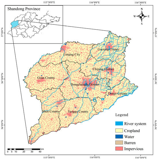
Figure 1.
The location of Liaocheng in Shandong.
2.2. Data Sources
Data on the amount of fertilizer application, labor, crop yield, and machinery used come from the Liaocheng Statistical Yearbook (2010–2022). Information on irrigation water comes from the Liaocheng Water Resources Bulletin (2010–2022) and the Shandong Water Resources Bulletin (2010–2022). The carbon data were calculated based on existing studies, and the carbon emission calculation for the water use system was derived from the research results of Zhao Rongqin [15] and Zuo Qiting [28].
2.3. Research Methods Carbon Emissions Accounting
Following Intergovernmental Panel on Climate Change (IPCC) Fifth Assessment Report guidelines, CH4 and N2O emissions are converted to CO2-equivalent values using 100-year global warming potential (GWP) coefficients of 28 and 265, respectively. Detailed calculation methodologies are presented in Table 1.

Table 1.
Formulas for carbon source and sink calculation.
Current carbon emission factors derive from internationally recognized sources. (1) Agricultural inputs: Fertilizer (nitrogen, phosphorus, potash) and pesticide (insecticides, herbicides, fungicides) coefficients established by the U.S. Oak Ridge National Laboratory (ORNL) through analysis of American agricultural production systems. ORNL, a premier national laboratory under the U.S. Department of Energy, is globally recognized as a leading authority in the fields of energy and environmental science. (2) Farming practices: Agricultural plastic mulch and tillage coefficients determined through joint research by the Institute of Agricultural Resources and Ecological Environment at Nanjing Agricultural University (IREEA) and the College of Biological Sciences at China Agricultural University (CABs). The coefficient was determined through field sampling in the North China Plain and is applicable to Liaocheng. Detailed emission coefficients for specific carbon sources are presented in Table 2.
Table 2.
Carbon emission factors.
2.4. System Dynamics
System dynamics, a methodology pioneered by Professor Jay W. Forrester at the Massachusetts Institute of Technology (MIT) in 1956, represents an interdisciplinary simulation framework grounded in feedback control theory and systems science. The standard workflow for applying system dynamics to address practical challenges involves three sequential phases: (1) defining the research problem; (2) constructing a boundary-constrained structural model with validation protocols; (3) conducting policy simulations through scenario analysis to identify optimal solutions. This study employs Vensim Personal Learning Edition (PLE) 10.0.0. software for model development and simulation.
2.5. Model Building
2.5.1. Modeling
The cyclical process of system dynamics is a specific dynamic simulation process tailored to the research direction, making the setting of system boundaries crucial for the accuracy of the system and the definition of the research content. This paper focuses on the agricultural production process and establishes causal feedback loops involving population, economy, and energy. Key variables of the system include agricultural machinery usage, agricultural inputs, carbon emissions, grain yield per unit area, grain production, grain planting area, and agricultural water use.
Based on the timeliness of the research and data availability, this study selects data from the past 13 years (2010–2022) as the research foundation to explore the constraint relationships within the system. It aims to predict resource demand over the seven years (2023–2030) under different development scenarios.
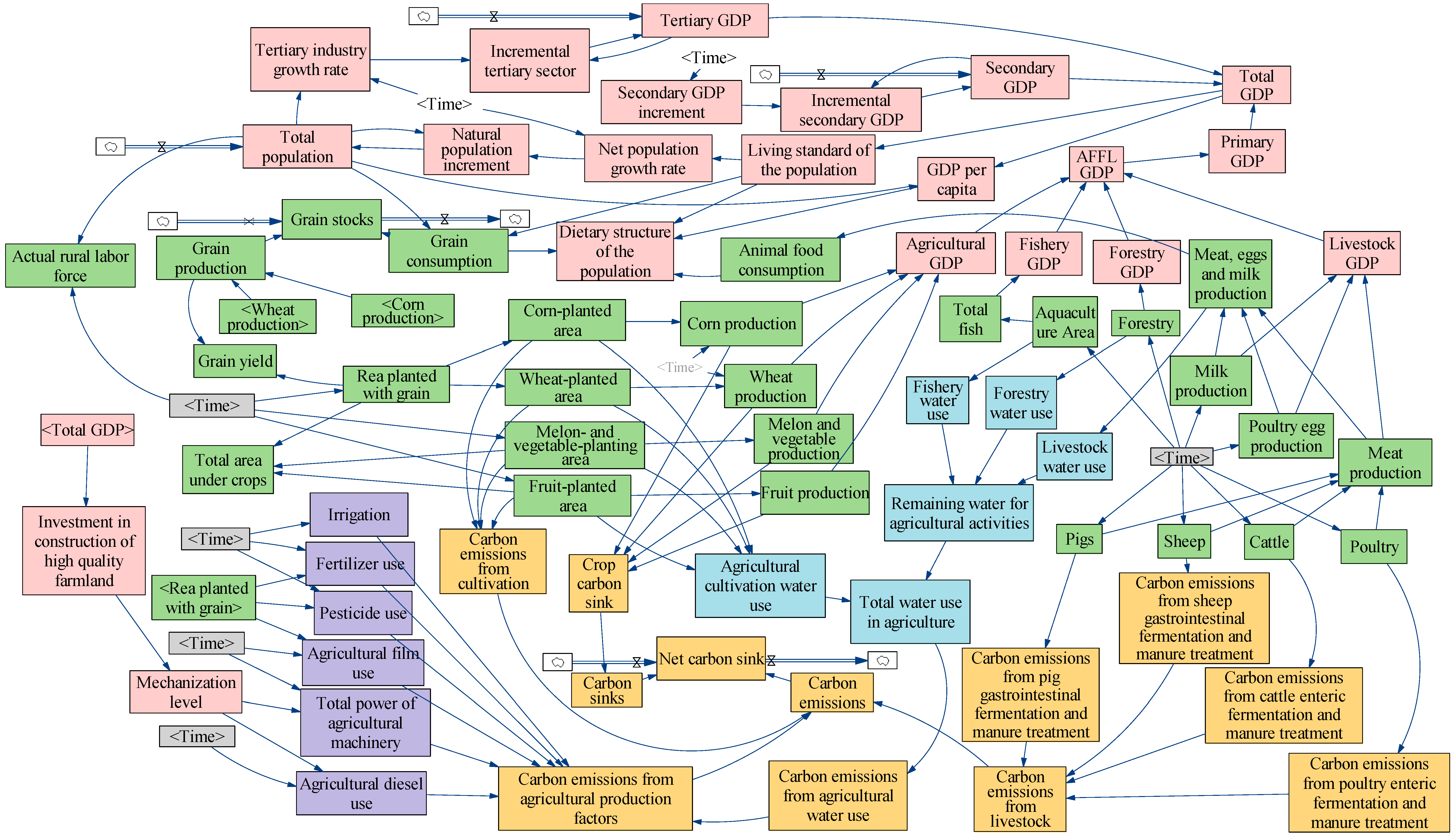
System flowchart is developed and constructed (Figure 2) based on the system structure, feedback mechanisms, and feedback loops. The flowchart systematically presents the dynamic structure and interaction mechanisms within the agricultural WEFC-Nexus system. In the diagram, each subsystem and its associated variables are represented in different colors: water, energy, food, carbon, and socio-economic indicators are represented in blue, purple, green, yellow, and pink, respectively, visually reflecting the interactions and hierarchical relationships among the system’s components. The SD model is displayed in Supplementary S1.

Figure 2.
System dynamics (SD) model of agricultural water–energy–food–carbon in Liaocheng.
2.5.2. Main Equations
The equations constructed based on the relationships of variables in the stock flow diagram are important components of the system dynamics model. The SD model of agricultural water–energy–food–carbon in Liaocheng contains 69 variables, and the equations of the main variables are selected for presentation. These are shown in Table 3. The model equations associated with each variable are presented in Supplementary S2.
Table 3.
Equations for the main variables.
2.5.3. Model Validation
The model’s accuracy is primarily evaluated through error analysis. This involves comparing the simulation results of the Liaocheng WEFC-Nexus system dynamics model with historical data to assess the model’s performance. The results indicate that when the relative error value is within 5% [30], the model’s simulation effect is considered good, and the model’s stability is deemed satisfactory. This study uses relative error (), coefffcient of determination (R2), coefffcient of variation (CV), root mean square error (RMSE), and mean average error (MAE) to evaluate the accuracy of the model. MAE and RMSE metrics are used to assess the difference between simulated and observed values. Smaller MAE and RMSE values indicate higher model accuracy. However, MAE and RMSE are influenced by dimensions and should be considered alongside other indicators to assess model stability.
where θ is the error value, X1i is the predicted value, and X2i is the history value.
A structurally stable model with good robustness is insensitive to changes in most parameters. This paper studies the sensitivity of the model by adjusting the input values of the parameters and observing the effect of parameter changes on the output variables of the model. The sensitivity calculation formula is as follows:
where S is the sensitivity of the output variable Q to the parameter; X0 and Q0 are the values of X and Q under the initial conditions; ΔX and ΔQ are the absolute values of the change in X and the corresponding change in Q, respectively.
In actual calculations, multiple state variables (i.e., multiple time points) are involved. To enhance the accuracy of the sensitivity analysis, k sets of parameter changes (ΔX) are selected, and sensitivity is calculated for each set, with the results then averaged. Thus, the average sensitivity of any parameter X across different states is defined as follows:
where SX is the average sensitivity of parameter X; k is the number of parameter changes; T is the time order, i.e., the number of time points; represents the sensitivity of parameter X at the jth time point in the ith group of parameters.
The model’s final output variable is selected to test sensitivity when parameter changes occur. During the model’s historical period (2010–2022), parameter is altered (increased or decreased by 10% and 20% annually), and the model is run under these conditions, along with the original scenario, to generate a total of five data sets. Sensitivity is then calculated using Formulas (6) and (7).
2.6. Scenario Setting
The scenarios in this paper are based on current research on the factors influencing carbon emissions and are set out as follows:
Scenario 1 (S1): Business-as-usual scenario, no policy intervention, i.e., predictions based on past data.
Scenario 2 (S2): Ideal development scenario: According to Liaocheng’s “14th Five-Year Plan” for the modernization of agriculture and rural areas, each variable is modified, and the policy proposes that by 2025, the comprehensive grain production capacity will be guaranteed to exceed 5.5 million tons. The output of meat, eggs, and milk will stabilize at more than 1.1 million tons, the area of aquaculture will stabilize at over 4000 hectares, and the area of planted green vegetables will exceed 210,000 hectares. The area under cultivation will increase to more than 210,000 hectares, with a total output of about 1.36 million tons. The efficiency of agricultural capital use will be improved, the construction of highly efficient water-saving irrigation will be strengthened, and the goal of adding 114,000 hectares of water-saving irrigation area by 2030 will be achieved.
Scenario 3 (S3): Strengthening agricultural investment development, adjusting the structure of food crops, and increasing crop yields based on the ideal development scenario. This scenario aims to realize a 5% increase in food production and a 10% increase in meat, egg, and milk production compared to the ideal scenario.
Scenario 4 (S4): Strengthening energy conservation and emission reduction development, under the ideal development situation, by improving the efficiency of agricultural fertilizer and pesticide use, as well as the efficiency of agricultural film use. This will reduce the use of chemical fertilizers, agricultural films, and pesticides by 5%.
The detailed scenario designs and key parameter changes are provided in Supplementary S2.
3. Results
3.1. Model Validation Results
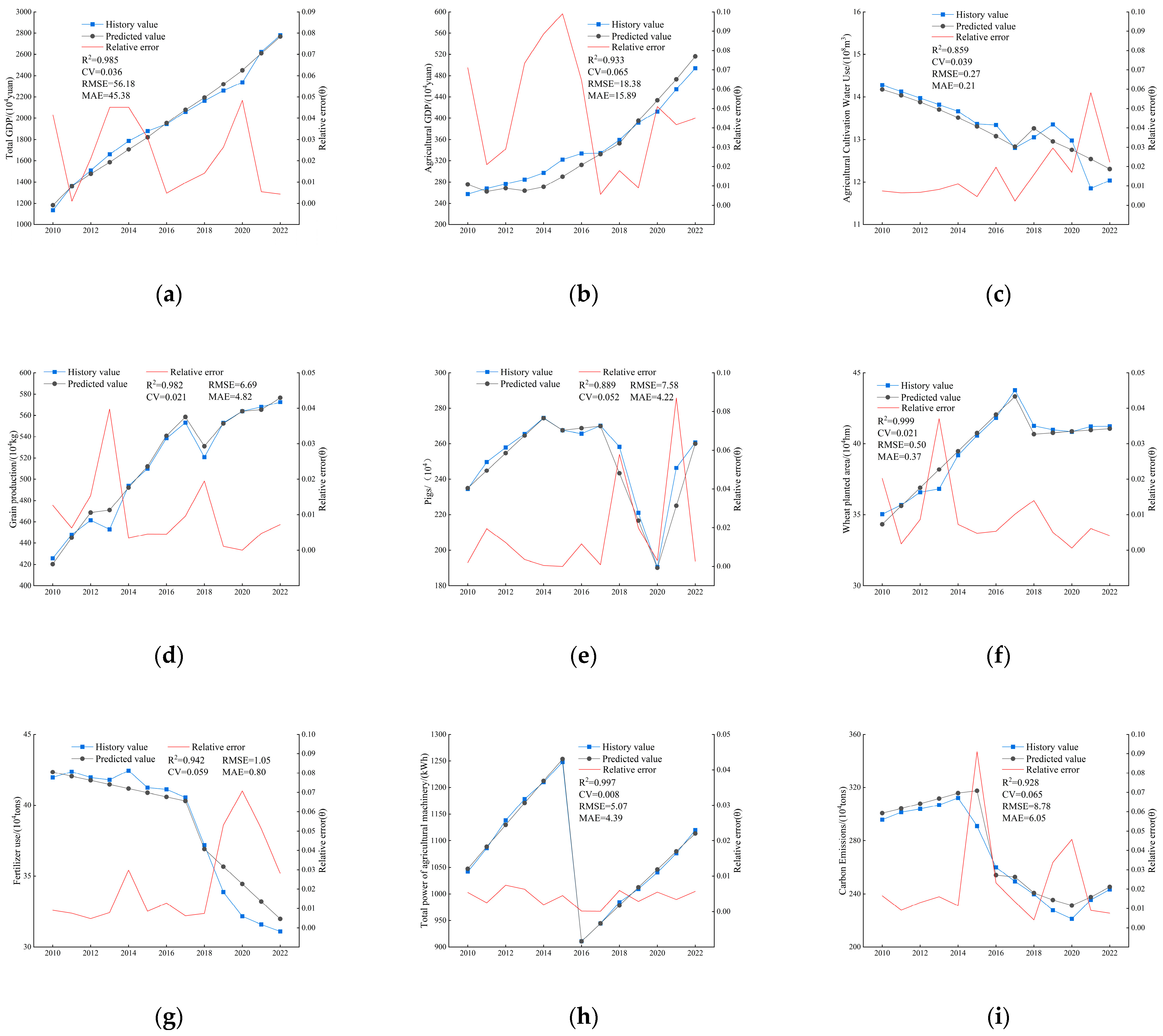
This study constructed the model using the equations in Table 3. Indicators were selected from five aspects—economic output, agricultural structure, water input, agricultural input, and carbon emissions—to evaluate the effectiveness of the model. For economic output, the following indicators were selected: total GDP, agricultural GDP, and grain production. For agricultural structure, the following indicators were selected: wheat-planted area and pigs. For water use, the following indicator was selected: agricultural cultivation water use. For agricultural input, the following indicators were selected: fertilizer use and total power of agricultural machinery. Each selected variable represents the most fundamental and essential characteristic or input/output indicator of the WEFC-Nexus system. The results are shown in Figure 3.
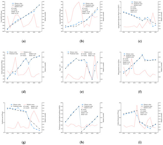
Figure 3.
Error values of main variables: (a) Total GDP, (b) Agricultural GDP, (c) Agricultural cultivation Water use, (d) Grain production, (e) Pigs, (f) Wheat-planted area, (g) Fertilizer use, (h) Total power of agricultural machinery, (i) Carbon emissions.
The results indicate that the simulated data for these variables aligned closely with the historical data in both values and trends, maintaining a relative error margin within 5%. The R2 values all exceeded 0.85, indicating minimal differences between the actual and simulated data [31]. Furthermore, the CV values for all the variables are close to zero, confirming that the model effectively simulated the dynamic development of agricultural carbon emissions in Liaocheng. The results indicate that some factors exhibit high RMSE and MAE values. However, when considered alongside other core indicators, the model still demonstrates effective fitting to the variables. The constructed SDM for Liaocheng exhibited robust simulation performance, providing a reliable foundation for future scenario simulations. For details of the calculation results for each parameter, please refer to Table S3.
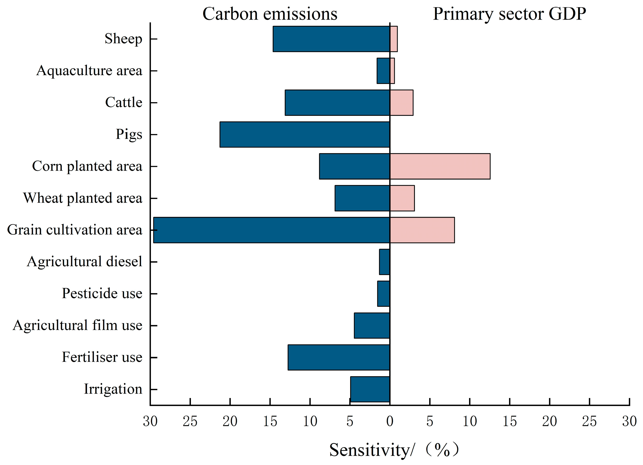
Figure 4 presents the sensitivity of carbon emissions and primary sector GDP to various parameters. These parameters were selected from three key areas: agricultural inputs, crop cultivation, and livestock. These factors were chosen for sensitivity analysis due to their critical role in the agricultural WEFC-Nexus system and their potential for policy intervention. As direct drivers of agricultural carbon emissions, analyzing their sensitivity provides insights into the primary factors influencing carbon emissions. Additionally, these factors underpin the model’s structure. The selected parameters reflect agricultural resource input conditions, cropping structure, and livestock composition, collectively representing the fundamental agricultural conditions in Liaocheng. In the scenario development, the analysis focused on modifying these core variables to assess their impact.
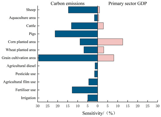
Figure 4.
Statistical figure of variable sensitivity analysis results.
The sensitivity analysis reveals that the factors with the greatest impact on carbon emissions are the grain cultivation area and the populations of pigs and sheep. The factor that is most influential on the GDP of the primary sector is the area dedicated to corn cultivation. The sensitivity of most of the parameters is less than 10%, indicating that the system is not sensitive to changes in most of the parameters. The parameters with higher sensitivity are the key factors that significantly influence the system. Based on the historical validation and sensitivity analysis of the model, it can be concluded that the model possesses good stability and is suitable for simulating real-world systems. For details of the calculation results for each parameter, please refer to Table S4.
The model developed in this paper integrates multiple factors and analyzes dynamic data to explore the feedback mechanisms of carbon emissions within agricultural systems. However, it places greater emphasis on the agricultural production process, and certain influencing factors have not been fully accounted for. This study assumes a stable and orderly future, with the system evolving at a consistent rate of change. In reality, however, future developments may be uncertain, and unexpected situations may arise. In the future, we will focus on reconstructing the mathematical relationships between various factors to better align the model with actual conditions, thereby improving the system dynamics approach.
3.2. Analysis of Trends in Agricultural Carbon Emissions
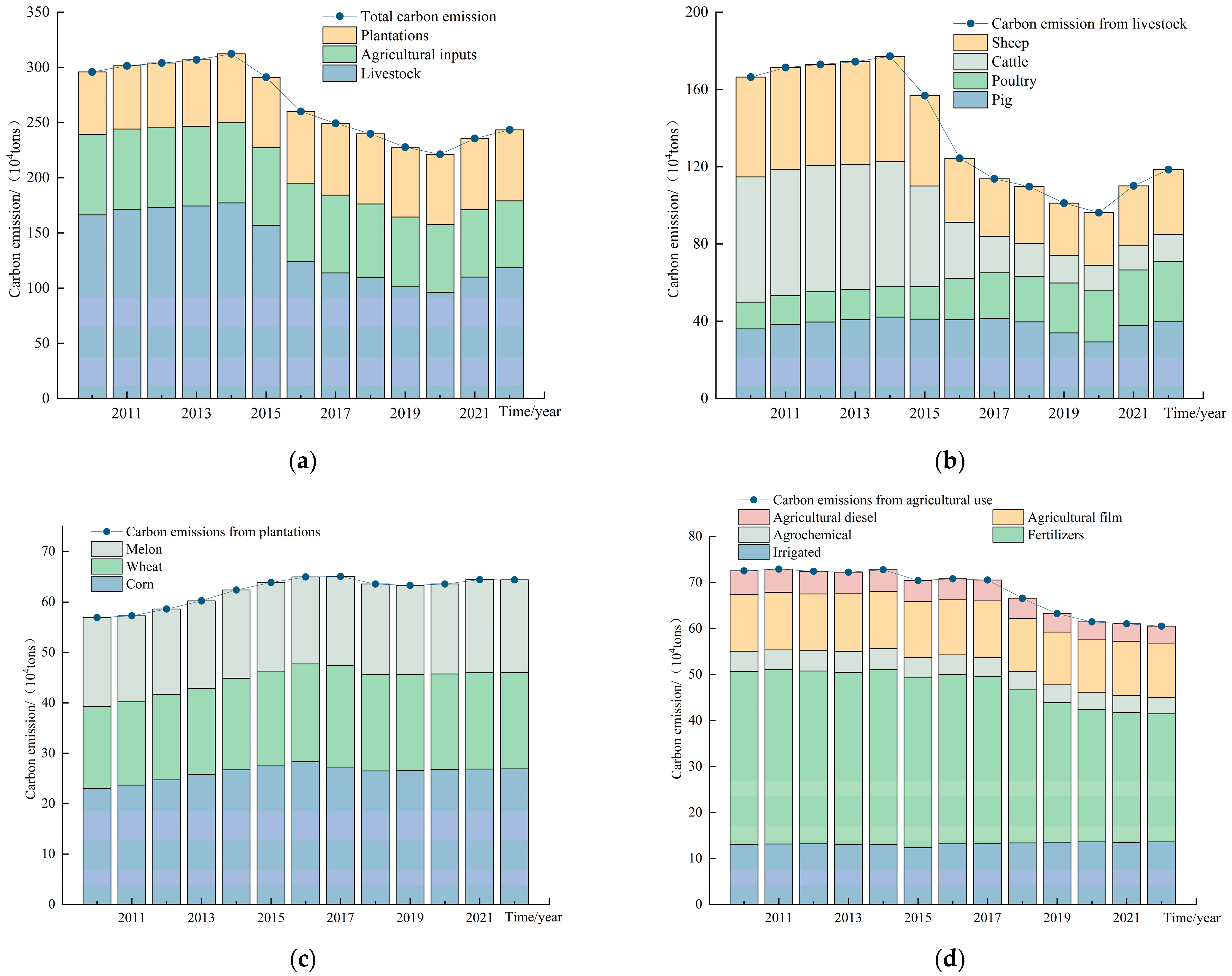
From Figure 5a, we can see that during the period of 2010–2022, the total amount of agricultural carbon emissions in Liaocheng presented a three-stage trend of “growth–sudden drop–steady rise,” reaching a peak of 3.12 million tons in 2014. It then gradually declined, but after 2020, it showed an overall rising trend, with agricultural carbon emissions reaching 2.46 million tons in 2022. In 2022, agricultural carbon emissions amounted to 2.46 million tons, with the livestock industry having the greatest impact. Its emissions accounted for nearly 50% of the total agricultural carbon emissions, followed by emissions from agricultural utilization (27%) and plantation (23%). This demonstrates that the implementation of carbon emission reduction policies in Liaocheng has had a remarkable effect, and agriculture is transitioning into a low-carbon, conservation-oriented green agriculture model.
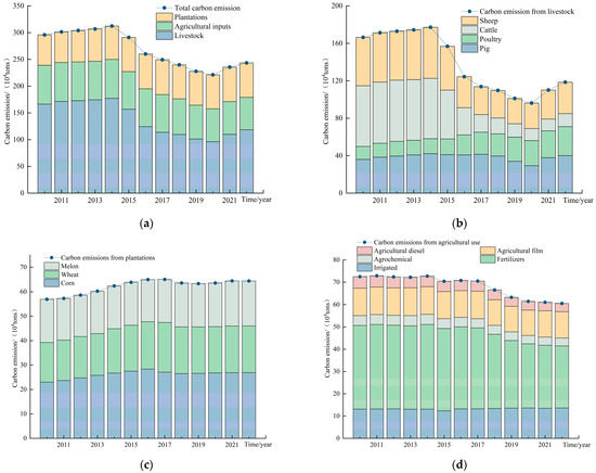
Figure 5.
Structure of carbon emissions, 2010–2022: (a) Agricultural total carbon emissions; (b) Carbon emissions from livestock farming; (c) Carbon emissions from crop cultivation; (d) Carbon emissions from agricultural inputs.
The estimation of carbon emissions from the livestock industry in Liaocheng mainly considered two major sources: livestock and poultry gastrointestinal fermentation, and the livestock and poultry manure management system. Liaocheng is a traditional livestock city with a wide variety of breeds, including pigs and poultry, which are heavily concentrated in the province. Livestock industry carbon emissions fluctuate annually, primarily influenced by the number of cattle (Figure 5b). Emissions reached a peak of 1.7718 million tons in 2014. However, after 2015, industrial structure adjustments within the livestock sector, including a reduction in cattle stock, led to a clear downward trend in emissions, reaching a minimum of 962,200 tons in 2020. The establishment of no-farming zones in 2015 and the implementation of mandatory manure treatment standards in 2018 have effectively reduced carbon emissions from the livestock industry in Liaocheng, steering the industry toward a greener and more sustainable transformation. The livestock industry accounts for nearly 50% of agricultural carbon emissions. Ensuring the high-quality development of the livestock industry while achieving green development in Liaocheng is a key issue that needs to be addressed.
Liaocheng is a major grain-producing area, with wheat and corn as the primary grain crops. These crops are also the main sources of carbon emissions from planting. The estimation of crop carbon emissions in Liaocheng primarily considered wheat, corn, and vegetables, the three major crops. The planting area has a significant impact. The growth from 2010 to 2016 was large, with an average annual growth rate of 2%, resulting in an increase of nearly 80,000 tons of carbon emissions over seven years, reaching a peak of 649,400 tons in 2016 (Figure 5c). However, the annual growth rate stabilized after 2016, with an average annual growth rate of −0.14%.
Carbon emissions from agricultural inputs showed a downward trend year by year, and in 2022, carbon emissions from agricultural inputs decreased by 16.1% compared to 2010. This indicates that Liaocheng has implemented a series of measures to improve the utilization efficiency of fertilizers, pesticides, agricultural films, and other agricultural inputs over the past 13 years, achieving a reduction in carbon emissions from agricultural inputs. Regarding internal carbon sources, the average proportion of carbon emissions over the past 13 years is as follows (Figure 5d): fertilizer (50.44%) > agricultural irrigation (19.40%) > agricultural film (17.59%) > agricultural diesel (6.49%) > pesticides (6.08%). Among these, fertilizer carbon emissions dominate, followed by agricultural irrigation and agricultural films, reflecting the essential role of these three factors in agricultural production. Pesticides contribute a relatively small percentage of carbon emissions but are still part of the overall agricultural input carbon emissions. A clear understanding of the structure of carbon emissions from agricultural inputs can help us better grasp the contribution of each agricultural factor to carbon emissions and provide an important basis for the formulation of targeted emission reduction policies and technological innovations.
3.3. Analysis of Agricultural Forecast Development Under Each Scenario
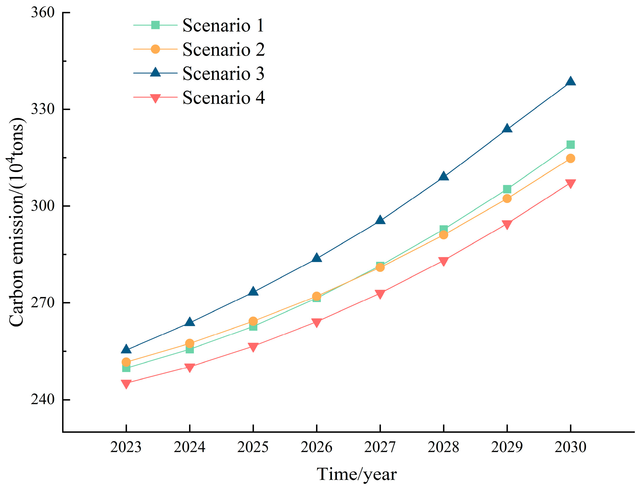
An analysis of Figure 6 shows the relationship between the size of carbon emissions under the four scenarios: S3 > S1 > S2 > S4. Liaocheng’s 14th Five-Year Plan policy adoption can more effectively reduce carbon emissions by 2030 than the conventional scenarios, with a reduction of nearly 4583.8 tons. The policy focuses on the optimization of the grain cultivation structure, the construction of high-quality farmland, and the improvement of the efficiency of the use of agricultural resources. S3 focuses solely on the development of agricultural reinforcement, and pursues the improvement of grain production, which increases carbon emissions by nearly 4.5% compared to S1. S4 can effectively reduce carbon emissions, and the reduction in agricultural input volume makes the agricultural carbon emissions have a significant reduction.
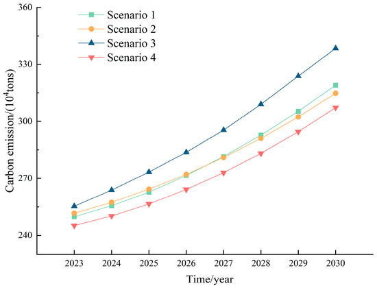
Figure 6.
Carbon emission projections by scenario. Scenario 1 (S1): Business-as-usual scenario; Scenario 2 (S2): Ideal development scenario; Scenario 3 (S3): Strengthening agricultural investment development; Scenario 4 (S4): Strengthening energy conservation and emission reduction development.
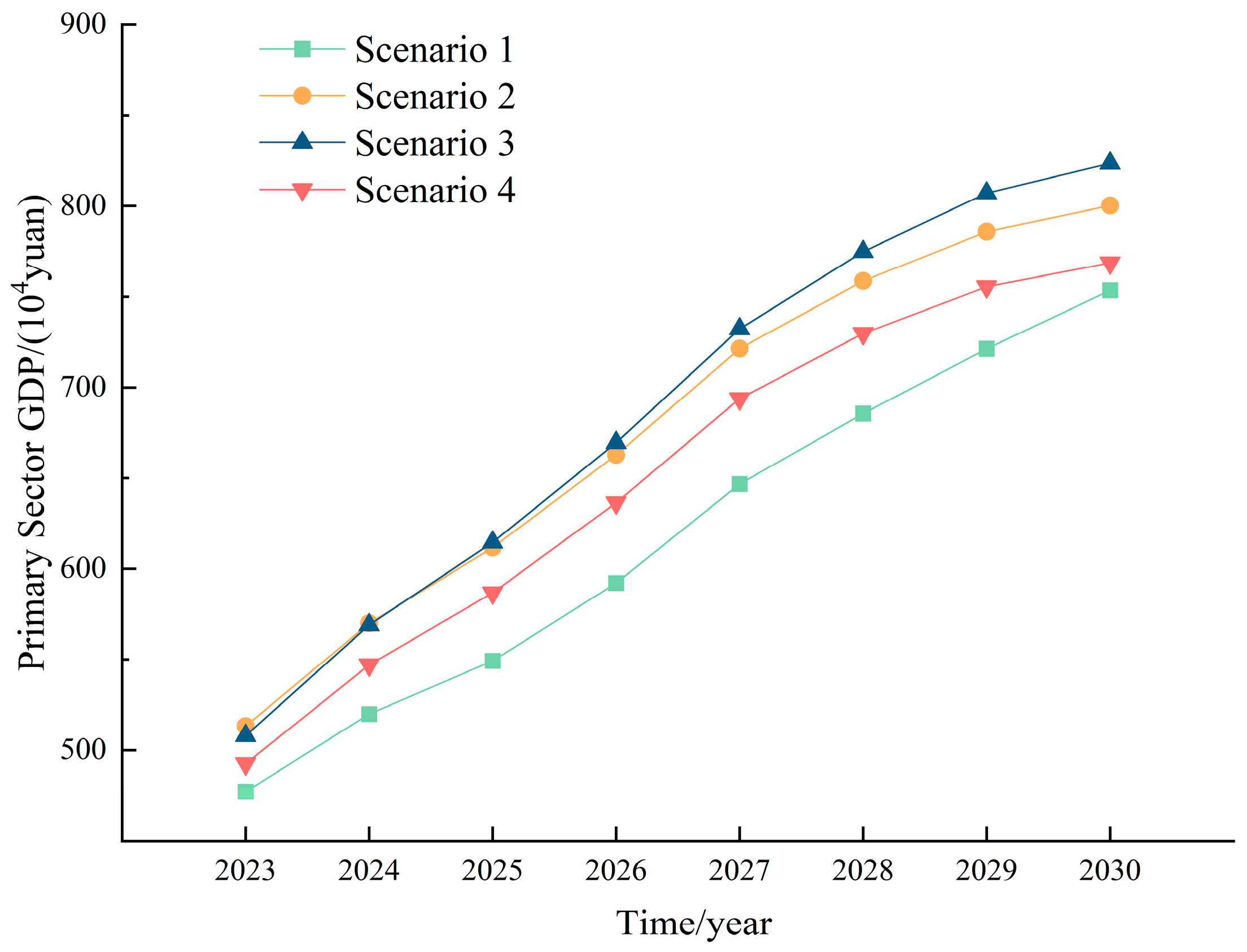
An analysis of Figure 7 shows that the size of the primary sector GDP relationship is ranked as follows: S3 > S2 > S4 > S1. S1 does not involve any policy interventions, with the irrational planning of farmland use, as well as agricultural input, leading to the lowest GDP compared to the other scenarios; S2 is ideal, and with the support of the 14th Five-Year Plan policy, primary sector GDP has increased to a large extent; S3 strengthens the development of agricultural investment, focusing on agricultural development, and primary sector GDP has increased by 10.06% compared to S1 and nearly 1.36% compared to S2, significantly improving the economic level of agricultural development; S4 strengthens the development of energy conservation and emission reduction, and the reduction in agricultural inputs such as fertilizers, pesticides, and agricultural films affects the primary sector GDP at the same time, so that the primary sector GDP has a small reduction compared with S2.
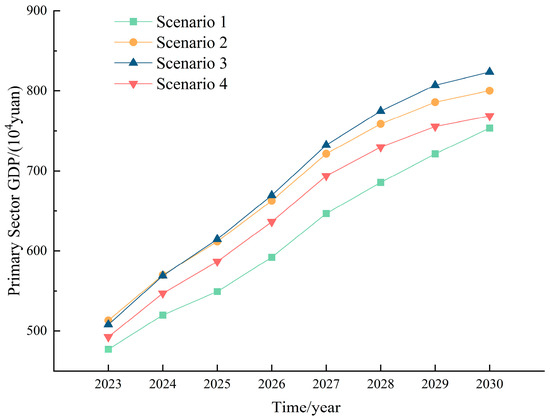
Figure 7.
Primary sector GDP industry forecast by scenario. Scenario 1 (S1): Business-as-usual scenario; Scenario 2 (S2): Ideal development scenario; Scenario 3 (S3): Strengthening agricultural investment development; Scenario 4 (S4): Strengthening energy conservation and emission reduction development.
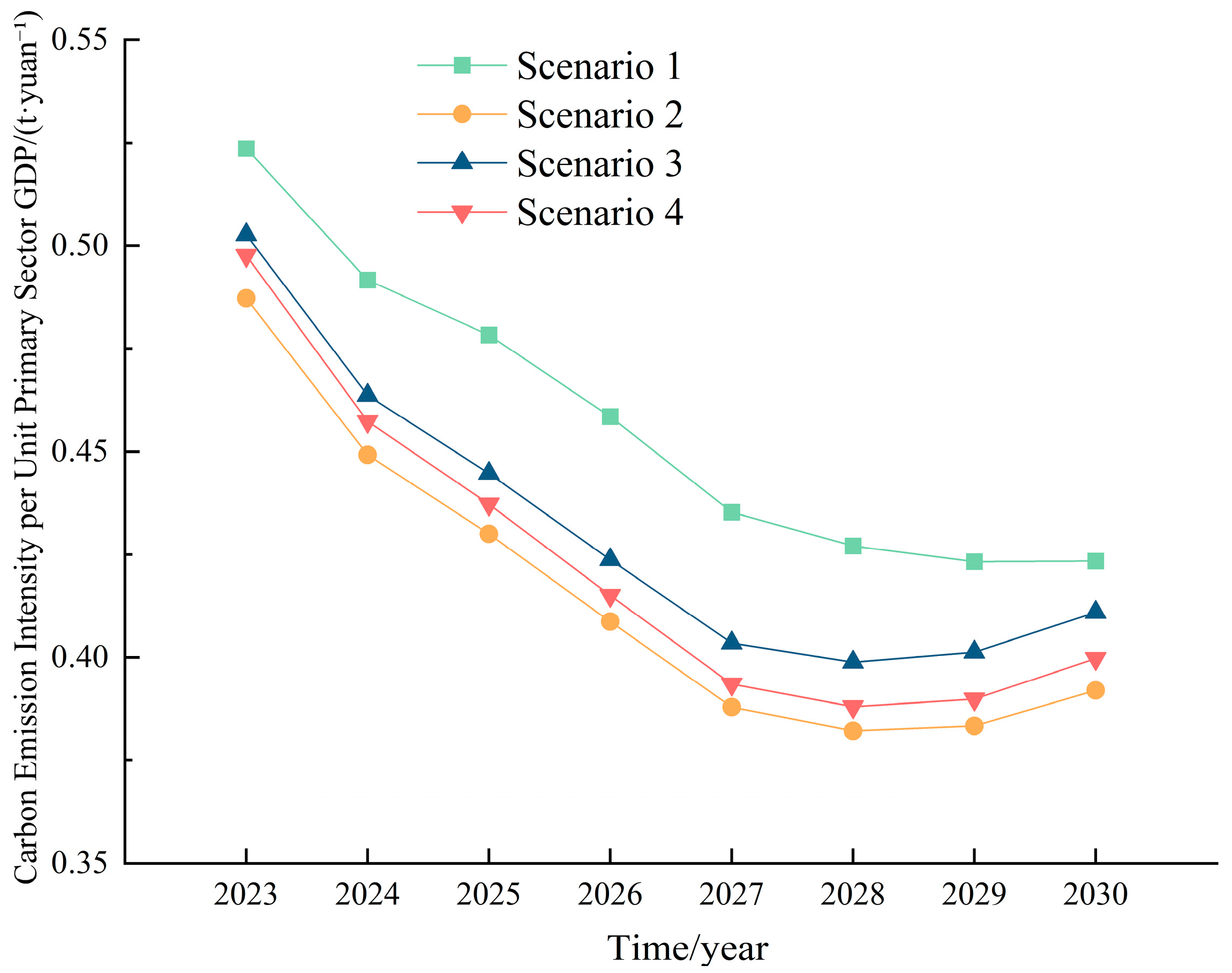
Based on the predictions of carbon emissions and primary sector GDP, we calculated the carbon emissions per unit of primary sector GDP (CEAG) to evaluate the relative merits of each scenario. The results are shown in Figure 8. By analyzing the average results for the CEAG, the following order of magnitude emerges: S2 < S4 < S3 < S1. The CEAG in S2 is 8.89% lower than in S1, ranking first among the four scenarios. This indicates that S2 effectively balances agricultural production with low-carbon goals. S3 and S4 show carbon intensities per unit of agricultural output that are 5.79% and 7.72% lower than in S1, respectively.
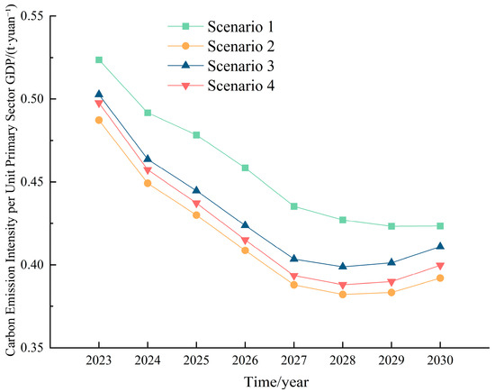
Figure 8.
Carbon emission intensity per unit primary sector GDP. Scenario 1 (S1): Business-as-usual scenario; Scenario 2 (S2): Ideal development scenario; Scenario 3 (S3): Strengthening agricultural investment development; Scenario 4 (S4): Strengthening energy conservation and emission reduction development.
When the agricultural development of Liaocheng is comprehensively analyzed from both ecological and economic perspectives, combining carbon emissions and primary sector GDP, it can be seen that the pursuit of economic development will occur at the cost of carbon emissions surging and environmental degradation, but only focusing on environmental protection and simply reducing agricultural inputs, will also inhibit the development of the agricultural economy to a certain extent. In summary, the ideal scenario of S2 can both control carbon emissions and realize the increase in primary industry production. How to balance the relationship between the environment and economic development is an area that needs to be emphasized in future policy formulation.
4. Discussion
4.1. Impact of Different Scenarios on WEFC-Nexus System
S1: Under natural development without policy intervention, this scenario not only fails to control carbon emissions but also shows a limited contribution to primary sector GDP growth. Carbon emissions are projected to reach 3.19 million tons by 2030, while the average annual growth rates of agriculture, forestry, animal husbandry, and fishery outputs remain stagnant at 1.2%. Persistent reliance on historical development paths would result in a “high-carbon lock-in” effect. Under this scenario, the carbon emission intensity in 2030 (0.42 tons/CNY) would fall short of Liaocheng’s 14th Five-Year Plan.
S2: This scenario achieves synergistic optimization of economic and environmental outcomes through full implementation of the 14th Five-Year Plan targets, effectively controlling carbon emissions while boosting primary industry output. However, its significant comprehensive benefits depend on high initial investments (e.g., smart drip irrigation systems costing CNY 1200 per mu) that require support from an Ecological Compensation Fund [10].
S3: With intensified agricultural investment focusing on food security, this approach achieves a 5% increase in grain production and 10% growth in meat/egg/milk outputs, but at the cost of surging carbon emissions (3.384 million tons). This reveals the inherent paradox between production enhancement and emission reduction [32], particularly regarding technological innovations for food security under natural resource constraints.
S4: This energy-efficient S achieves a 3% carbon reduction through agricultural input restrictions, mainly due to smallholders’ limited capacity for technological adaptation [10]. Implementing [20] a multi-sectoral synergy framework through water-saving irrigation subsidies linked to carbon allowances could mitigate equity pressures in policy execution.
The holistic analysis reveals strong water–carbon coupling: irrigation energy consumption accounts for 19.4% of agricultural emissions, while water efficiency dominates interannual carbon balance variations in terrestrial ecosystems [33]. Promoting water-saving technologies therefore constitutes the key to resolving the water–carbon dilemma while balancing environmental and economic objectives.
4.2. Policy Implications
(1) Developing low-carbon animal husbandry. As the primary source of agricultural carbon emissions, animal husbandry requires focused improvements in breeding technology, feed optimization, and manure management in Liaocheng—a traditional livestock hub. It is recommended to reduce methane gas emissions from livestock animals, and to carry out technological innovation to recycle and treat the methane generated. The biogas-based recycling model is an effective means to achieve efficient conversion of biomethane from poor-quality biomass and is an effective means to save energy and reduce emissions [34]. For example, it is recommended to adopt a biogas circular economy model for pig farming. This approach delivers high environmental and economic benefits. Based on carbon trading, the adoption of the circular economic model in pig farming could generate an economic benefit of CNY193 million [16]. An additional recommendation is to develop more productive pastures and use these to replace low-productivity pastures. This reduces greenhouse gas emissions [35]. Optimizing manure management can reduce the nitrogen footprint by more than 30% [36], and choosing a more advanced and scientific manure management system is also of great importance.
Although low-carbon livestock farming offers significant benefits in resource recycling, its development faces several challenges. First, the cost of transitioning to low-carbon practices is high. Second, the adoption of environmentally friendly production methods by farmers remains limited. Third, supportive measures are insufficient, and external assistance is lacking. To promote low-carbon livestock farming, the government should implement policies that combine mandatory regulations with incentives. These policies should focus on promoting low-carbon practices and supporting industry participants in adopting standardized farming methods. As the scale of low-carbon livestock farming grows, rural areas should develop long-term strategies for high-quality development. Relevant departments must provide ongoing support to ensure sustainability.
(2) Adjustment of the agricultural structure. Under the premise of guaranteeing food security, combined with the actual situation of agricultural production and market demand, the optimization of the agricultural industrial structure should be carried out. Studies show that increasing crop density stabilizes yield. It also reduces greenhouse gas emissions [37]. Mixed-crop layouts from Heilongjiang Province offer solutions. These methods are replicable [18]. Agricultural structural adjustment can reduce carbon emissions while facilitating the gradual decoupling of economic growth from agricultural carbon emissions [38]. However, achieving complete decoupling requires continuous optimization of the agricultural structure. It is also crucial to recognize that structural adjustments may incur opportunity costs, generate positive externalities, and result in direct economic losses. Therefore, a systematic strategy for structural adjustment must be established, along with a supporting policy and legal framework, to enable effective macro-regulation. It is recommended to reasonably adjust the proportion of agriculture and animal husbandry, consider the combination of planting and raising, and develop local specialty agriculture. In the agricultural sector, efforts should focus on expanding the cultivation scale of key crops and strengthening the market presence of the “Liaocheng Three Treasures,” which include donkey hide gelatin, reishi mushrooms, and mulberry mushrooms. In the livestock sector, a distinctive livestock system known as the “Three Blacks, Two Whites, and One Yellow” should be established. The “Three Blacks” refer to black-haired donkeys, black-headed sheep, and Yellow River black cattle; the “Two Whites” refer to white rabbits and white pigeons; and the “One Yellow” refers to Lu Xi yellow cattle. High-quality farmland construction should be undertaken, and grain yields should be improved.
(3) It is recommended to enhance the efficiency of the use of agricultural materials, increase capital investment in agricultural technology, achieve a reduction in the amount of chemical fertilizers and pesticides and increase efficiency, levy a higher value-added tax (VAT) on fertilizer producers, while exempting organic fertilizers from VAT, and, where possible, use animal manure to replace traditional fertilizers [39], or dig deeper into the value of applying compost from planting and farming wastes to increase the recycling rate of nitrogen [40], phosphorus, and potassium. From a cost–benefit perspective, the use of organic fertilizer by farmers is expected to increase the average profit per acre by USD 60.70 [41]. It is recommended to improve mechanization, develop biomass energy, and reduce the use of heavy polluting agricultural machinery. Concurrently, the expansion of water-saving irrigation infrastructure must be accelerated. Although investments in water-saving irrigation projects enhance yields and efficiency, the direct economic benefits do not fully offset the initial investment costs. The 10-year average annual return on investment for water-saving irrigation projects in food production ranges from CNY −0.52 to CNY 0.21. However, when considering the broader economic spillover effects, the overall return on investment is much higher. The combined return, accounting for both the industry-wide benefits and the savings in water usage within the plantation sector, yields a net return on investment ranging from CNY 0.60 to CNY 5.55 [42] after deducting the initial investment costs.
Water-saving irrigation projects offer substantial economic and environmental benefits, playing a critical role in fostering sustainable agricultural development. The development of water-saving irrigation technology faces several challenges, including limited technological adaptability, low farmer acceptance, and inadequate policy and funding support. Future progress should focus on technological innovation, cost control, and regional adaptability, particularly in promoting the widespread use of smart irrigation systems. Additionally, the government should enhance policy support by providing farmers with accessible technical training and financial assistance to facilitate the adoption of efficient water-saving technologies. Only through coordinated development in technology, policy, and management can agricultural water use efficiency be significantly improved.
5. Conclusions
This study establishes a WEFC-Nexus model for the agricultural production process on the basis of the fine accounting of agricultural carbon emissions, using Liaocheng as a case study. The carbon emissions in the agricultural production process in Liaocheng were specifically split to understand the situation. Considering the specific conditions of the study area and the local development plan, four scenarios were developed. Through simulation and analysis, the carbon emissions and economic development of Liaocheng under different scenarios were studied. The key conclusions are as follows:
(1) By calculating and analyzing the carbon emissions from the agricultural production process in Liaocheng, it can be seen that the total agricultural carbon emissions in Liaocheng showed a three-stage trend of “growth–plunge–steady rise” between 2010 and 2022, and reached a peak of 3,125,200 tons in 2014. Specifically, animal husbandry had the greatest impact, and its emissions account for nearly 50% of the total agricultural carbon emissions. This is followed by agricultural utilization emissions (27%) and plantation emissions (23%). From the point of view of the total carbon emissions from livestock, the reason for the fluctuation is mainly focused on the changes in cattle stock. In terms of carbon emissions from cultivation, the annual growth rate stabilized after 2016. In terms of carbon emissions from agricultural input supplies, the average carbon emission ratio over the past 13 years is as follows: fertilizer (50.44%) > agricultural irrigation (19.40%) > agricultural film (17.59%) > agricultural diesel (6.49%) > pesticides (6.08%), with fertilizer carbon emissions dominating.
(2) Through the scenario simulation prediction analysis, the carbon emission size relationship under four scenarios was obtained as S3 > S1 > S2 > S4, and the size relationship of the primary industry output value is S3 > S2 > S4 > S1. The size relationship of the CEAG is S2 < S4 < S3 < S1. The CEAG for S2, S3, and S4 decreased by 8.86%, 5.79%, and 7.72%, respectively, compared to S1. S2 can control carbon emission and realize the increase in the output of the primary industry at the same time. The future agricultural policy of Liaocheng should consider both economic development and ecological protection. The policy focus should be on developing low-carbon livestock, restructuring agriculture and improving the efficiency of agricultural utilization.
(3) Future research should focus on two key areas. First, improving the precision of carbon emission factor systems. Currently, emission factors rely heavily on international databases, such as the ORNL fertilizer coefficients, which have not been sufficiently validated locally. In situ monitoring technologies can be employed to analyze the nonlinear effects of variables such as soil pH, tillage patterns, and feed conversion efficiency on carbon source/sink intensity in agricultural soils in Liaocheng, allowing for the development of a dynamically updated, localized factor database. Then, further investigation into the impact of climate change on the system is needed. Understanding the effects of climate change on agricultural production will enable the adoption of scientifically sound and effective strategies to enhance agricultural resilience and promote sustainable development.
Supplementary Materials
The following supporting information can be downloaded at https://www.mdpi.com/article/10.3390/su17146607/s1. Supplementary S1: S1-Model; Supplementary S2: S2-model equations; Table S3: Error values of main variables; Table S4: Statistical table of variable sensitivity analysis results.
Author Contributions
Conceptualization, Y.L. and H.W.; methodology, Y.L.; software, W.Y.; validation, W.Y.; formal analysis, W.Y.; resources, Y.L.; data curation, W.Y.; writing—original draft preparation, W.Y.; writing—review and editing, Y.L., W.Y., and S.H.; supervision, Z.X. and S.H.; project administration, X.C.; funding acquisition, Y.L. All authors have read and agreed to the published version of the manuscript.
Funding
This research was funded by the Social Science Planning Project of Shandong Province (No. 23CGLJ04); Philosophy and Social Sciences Research Project for Higher Education Institutions of Shandong Province (No. 2024ZSMS071); Postdoctoral Workstation of Shandong Institute of Water Resources Research (No. 2024-09); the Open Research Fund of Henan Key Laboratory of Water Resources Conservation and Intensive Utilization in the Yellow River Basin (No. HAKF202105; HAKF202202).
Institutional Review Board Statement
Not applicable.
Informed Consent Statement
Not applicable.
Data Availability Statement
Data are contained within the article.
Conflicts of Interest
The authors declare no conflicts of interest.
References
- Assa, N.; Ma, R.; Li, J.; Luo, H.; Zhao, Q.; Tomka, J.; Zhang, M. Tackling climate change in agriculture: A global evaluation of the effectiveness of carbon emission reduction policies. J. Clean. Prod. 2024, 468, 142973. [Google Scholar] [CrossRef]
- Wang, J.H.; Sun, S.K.; Yin, Y.L.; Wang, K.X.; Sun, J.X.; Tang, Y.H.; Zhao, J.F. Water-Food-Carbon Nexus related to the producer-consumer link: A review. Adv. Nutr. 2022, 13, 938–952. [Google Scholar] [CrossRef]
- Zhang, P.Y.; He, J.; Pang, B.; Lu, C.P.; Qin, M.Z.; Lu, Q.C. Temporal and spatial differences in carbon footprint in farmland ecosystem: A case study of Henan Province, China. Chin. J. Appl. Ecol. 2017, 28, 3050–3060. [Google Scholar]
- Tian, Y.; Yin, Y. Re-evaluation of China’s Agricultural carbon emissions: Basic status, dynamic evolution and spatial spillover effects. Chin. Rural Econ. 2022, 03, 104–127. [Google Scholar]
- Yuan, X.; Hua, L.C.; Wen, L.J.; Hui, L.; Yan, L.Q.; Lin, K.Z.; Peng, Y.; Jiahui, L. Analysis of spatial and temporal characteristics and drivers of agricultural carbon emissions in China. Chin. J. Eco-Agric. 2024, 32, 1805–1817. [Google Scholar]
- Qian, F.K.; Wang, X.G.; Gu, H.L.; Wang, D.P.; Li, P.F. Characteristics of spatial and temporal divergence of agricultural carbon emissions in three northeastern provinces and its key driving factors. Chin. J. Eco-Agric. 2024, 32, 30–40. [Google Scholar]
- Zhou, Y.F.; Li, B.; Zhang, R.Q. Spatiotemporal evolution and influencing factors of agricultural carbon emissions in Hebei Province at the county scale. Chin. J. Eco-Agric. 2022, 30, 570–581. [Google Scholar]
- Cao, Y.L.; Ni, X.; Gong, H.Y. Influencing factors and decoupling effects of agricultural carbon emissions in the Yangtze river economic belt. Huanjing Kexue 2025, 46, 1535–1547. [Google Scholar]
- Liu, Y.; Xu, S.X. Study on the impact of digital economy development on agricultural carbon emissions in China. Chin. J. Agric. Resour. Reg. Plan 2025, 46, 1–12. [Google Scholar]
- Shang, G.Y.; Yang, X. Impacts of policy cognition on low-carbon agricultural technology adoption of farmers. Chin. J. Appl. Ecol. 2021, 32, 1373–1382. [Google Scholar]
- Tang, J.; Lu, Y. Emission-reduction effect of green agricultural technology innovation in China. J. Agro-For. Econ. Manag. 2024, 23, 720–730. [Google Scholar]
- Geng, L.; Peng, L.T.; Wei, B.; An, Y. Impact of urbanization on agricultural carbon emission and its coupling relationship in the Yangtze river economic belt. Ecol. Econ. 2024, 40, 128–138. [Google Scholar]
- Hu, W.L.; Zhang, J.X.; Wang, H.L. Study on the characteristics and influencing factors of agricultural carbon emissions in china. Stat. Decis. 2020, 36, 56–62. [Google Scholar]
- Xu, Q.H.; Zhang, G.S. Spatial spillover effect of agricultural mechanization on agricultural carbon emission intensity: An empirical analysis of panel data from 282 cities. China Popul. Resour. Environ. 2022, 32, 23–33. [Google Scholar]
- Zhao, R.Q.; Liu, Y.; Tian, M.M.; Ding, M.L.; Cao, L.H.; Zhang, Z.P.; Chuai, X.W.; Xiao, L.G.; Yao, L.G. Impacts of water and land resources exploitation on agricultural carbon emissions: The water-land-energy-carbon nexus. Land Use Policy 2018, 72, 480–492. [Google Scholar] [CrossRef]
- Xue, Y.N.; Luan, W.X.; Wang, H.; Yang, Y.J. Environmental and economic benefits of carbon emission reduction in animal husbandry via the circular economy: Case study of pig farming in Liaoning, China. J. Clean. Prod. 2019, 238, 117968. [Google Scholar] [CrossRef]
- Ren, H.R.; Liu, B.; Zhang, Z.R.; Li, F.X.; Pan, K.; Zhou, Z.L.; Xu, X.S. A water-energy-food-carbon nexus optimization model for sustainable agricultural development in the Yellow River Basin under uncertainty. Appl. Energy 2022, 326, 120008. [Google Scholar] [CrossRef]
- Hu, M.M.; Tang, H.J.; Yu, Q.Y.; Wu, W.B. A new approach for spatial optimization of crop planting structure to balance economic and environmental benefits. Sustain. Prod. Consum. 2024, 53, 109–124. [Google Scholar] [CrossRef]
- Feng, T.T.; Liu, B.; Ren, H.R.; Yang, J.J.; Zhou, Z.L. Optimized model for coordinated development of regional sustainable agriculture based on water–energy–land–carbon nexus system: A case study of Sichuan Province. Energy Convers. Manag. 2023, 291, 117261. [Google Scholar] [CrossRef]
- Halbe, J.; Pahl-Wostl, C.; Lange, M.A.; Velonis, C. Governance of transitions towards sustainable development—The water–energy–food nexus in Cyprus. Water Int. 2015, 40, 877–894. [Google Scholar] [CrossRef]
- Li, G.H.; Chen, X.; You, X.Y. System dynamics prediction and development path optimization of regional carbon emissions: A case study of Tianjin. Renew. Sustain. Energy Rev. 2023, 184, 113579. [Google Scholar] [CrossRef]
- Du, S.P.; Liu, G.Y.; Li, H.; Zhang, W.; Santagata, R. System dynamic analysis of urban household food-energy-water nexus in Melbourne (Australia). J. Clean. Prod. 2022, 379, 113579. [Google Scholar] [CrossRef]
- Hussien, W.A.; Memon, F.A.; Savic, D.A. An integrated model to evaluate water-energy-food nexus at a household scale. Environ. Model. Softw. 2017, 93, 366–380. [Google Scholar] [CrossRef]
- Li, G.J.; Li, Y.L.; Jia, X.J.; Du, L.; Huang, D.H. Establishment and simulation study of system dynamic model on sustainable development of water-energy-food nexus in Beijing. Manag. Rev. 2016, 28, 11–26. [Google Scholar]
- Mi, H.; Zhou, W. The System Simulation of China’s grain, fresh water and energy demand in the next 30 years. Popul. Econ. 2010, 01, 1–7. [Google Scholar]
- Francisco, É.C.; Ignácio, P.S.d.A.; Piolli, A.L.; Dal Poz, M.E.S. Food-energy-water (FEW) nexus: Sustainable food production governance through system dynamics modelling journal of cleaner production. J. Clean. Prod. 2023, 386, 135825. [Google Scholar] [CrossRef]
- Jie, L.; Hongmei, L.; Yelong, Z.; Weishan, Q.; Mengwei, L.; Zhaorui, J. Input perspective-based decoupling of carbon emissions of agricultural land utilization and economic development in Shandong Province. Bull. Soil Water Conserv. 2016, 36, 303–308. [Google Scholar]
- Ting, Z.Q.; Guang, Z.C.; Xia, M.J.; Xi, Q.; Zhuo, Z.Z. Carbon dioxide emission equivalen analysis method of water resource behaviors and its application. South-North Water Transf. Water Sci. Technol. 2023, 21, 1–12. [Google Scholar]
- Min, J.S.; Hu, H. Calculation of greenhouse gases emission from agricultural production in China. China Popul. Resour. Environ. 2012, 22, 21–27. [Google Scholar]
- Chao, B.; Jie, W.H.; Siao, S. Comprehensive simulation of resources and environment carrying capacity for Urban Agglomeration: A system dynamics approach. Ecol. Indic. 2022, 138, 108874. [Google Scholar] [CrossRef]
- Purwanto, A.; Susnik, J.; Suryadi, F.X.; Fraiture, C.d. Quantitative simulation of the water-energy-food (WEF) security nexus in a local planning context in Indonesia. Sustain. Prod. Consum. 2021, 25, 198–216. [Google Scholar] [CrossRef]
- Mok, W.K.; Tan, Y.X.; Chen, W.N. Technology innovations for food security in Singapore: A case study of future food systems for an increasingly natural resource-scarce world. Trends Food Sci. Technol. 2020, 102, 155–168. [Google Scholar] [CrossRef]
- Jung, M.; Reichstein, M.; Schwalm, C.R.; Huntingford, C.; Sitch, S.; Ahlström, A.; Arneth, A.; Camps-Valls, G.; Ciais, P.; Friedlingstein, P.; et al. Compensatory water effects link yearly global land CO2 sink changes to temperature. Nature 2017, 541, 516–520. [Google Scholar] [CrossRef]
- Beer, C.; Reichstein, M.; Tomelleri, E.; Ciais, P.; Jung, M.; Carvalhais, N.; Rödenbeck, C.; Arain, M.A.; Baldocchi, D.; Bonan, G.B.; et al. Terrestrial gross carbon dioxide uptake: Global distribution and covariation with climate. Science 2010, 329, 834–838. [Google Scholar] [CrossRef]
- Gutiérrez-Peña, R.; Mena, Y.; Batalla, I.; Mancilla-Leytón, J.M. Carbon footprint of dairy goat production systems: A comparison of three contrasting grazing levels in the Sierra de Grazalema Natural Park (Southern Spain). J. Environ. Manag. 2018, 232, 993–998. [Google Scholar] [CrossRef]
- Ledgard, S.F.; Wei, S.; Wang, X.; Falconer, S.; Zhang, N.; Zhang, X.; Ma, L. Nitrogen and carbon footprints of dairy farm systems in China and New Zealand, as influenced by productivity, feed sources and mitigations. Agric. Water Manag. 2019, 213, 155–163. [Google Scholar] [CrossRef]
- She, W.; Wu, Y.; Huang, H.; Chen, Z.D.; Cui, G.X.; Zheng, H.B.; Guan, C.Y.; Chen, F. Integrative analysis of carbon structure and carbon sink function for major crop production in China’s typical agriculture regions. J. Clean. Prod. 2017, 162, 702–708. [Google Scholar] [CrossRef]
- Ding, D.; Liang, R. Construction of The rule of law system for the adjustment of agricultural structure in the northern farming-pastoral ecotone from the perspective of carbon reduction. Acta Agrestia Sin. 2025, 33, 1557–1566. [Google Scholar]
- Luo, Y.S.; Long, X.L.; Wu, C.; Zhang, J.J. Decoupling CO2 emissions from economic growth in agricultural sector across 30 Chinese provinces from 1997 to 2014. J. Clean. Prod. 2017, 159, 220–228. [Google Scholar] [CrossRef]
- Tie, J.Z.; Gao, X.Q.; Liu, Y.Y.; Chen, W.X.; Hu, L.L.; Yu, J.H.; Li, T.L. Improving the value of planting and breeding waste compost in agricultural applications: A zucchini cultivation case and circular agricultural models analysis. Chem. Eng. J. 2024, 496, 153984. [Google Scholar] [CrossRef]
- Jieyan, L.; Hongli, Z.; Huiqi, T. Impact of organic fertilizer application on farmers’ profit. J. Arid Land Resour. Environ. 2022, 36, 70–78. [Google Scholar]
- Xiangmin, L.; Yumei, Z. Economic and environmental impacts of water-saving irrigation projects in China. Chin. J. Agric. Resour. Reg. Plan. 2025, 46, 68–78. [Google Scholar]

Disclaimer/Publisher’s Note: The statements, opinions and data contained in all publications are solely those of the individual author(s) and contributor(s) and not of MDPI and/or the editor(s). MDPI and/or the editor(s) disclaim responsibility for any injury to people or property resulting from any ideas, methods, instructions or products referred to in the content. |
© 2025 by the authors. Licensee MDPI, Basel, Switzerland. This article is an open access article distributed under the terms and conditions of the Creative Commons Attribution (CC BY) license (https://creativecommons.org/licenses/by/4.0/).