Projected Urban Air Pollution in Riyadh Using CMIP6 and Bayesian Modeling

Abstract

Rapid urbanization and climate change pose significant challenges to air quality in arid metropolitan areas, with critical implications for public health and sustainable development. This study projects the evolution of air pollution in Riyadh, Saudi Arabia, through 2070 using an integrated modeling approach that combines CMIP6 climate projections with localized air quality data. We analyzed daily concentrations of major pollutants (SO₂, NO₂) across 15 strategically selected monitoring stations representing diverse urban environments, including traffic corridors, residential areas, healthcare facilities, and semi-natural zones. Climate data from two Earth System Models (CNRM-ESM2-1 and MPI-ESM1.2) were bias-corrected and integrated with historical pollution measurements (2000–2015) using hierarchical Bayesian statistical modeling under SSP2-4.5 and SSP5-8.5 emission scenarios. Our results revealed substantial deterioration in air quality, with projected increases of 80–130% for SO₂ and 45–55% for NO₂ concentrations by 2070 under high-emission scenarios. Spatial analysis demonstrated pronounced pollution gradients, with traffic corridors (Eastern Ring Road, Northern Ring Road, Southern Ring Road) and densely urbanized areas (King Fahad Road, Makkah Road) experiencing the most severe increases, exceeding WHO guidelines by factors of 2–3. Even semi-natural areas showed significant increases in pollution due to regional transport effects. The hierarchical Bayesian framework effectively quantified uncertainties while revealing consistent degradation trends across both climate models, with the MPI-ESM1.2 model showing a greater sensitivity to anthropogenic forcing. Future concentrations are projected to reach up to 70 μg m⁻³ for SO₂ and exceed 100 μg m⁻³ for NO₂ in heavily trafficked areas by 2070, representing 2–3 times the Traffic corridors showed concentration increases of 21–24% compared to historical baselines, with some stations (R5, R13, and R14) recording projected levels above 4.0 ppb for SO₂ under the SSP5-8.5 scenario. These findings highlight the urgent need for comprehensive emission reduction strategies, accelerated renewable energy transition, and reformed urban planning approaches in rapidly developing arid cities.

1. Introduction

Climate change and air pollution are two closely linked crises, both resulting from anthropogenic activities such as fossil fuel combustion, industrialization, rapid urbanization, and intensified transportation. Air pollution and climate change are among the most pressing environmental challenges of our time, with significant implications for human health, ecosystems, and societal stability worldwide [1,2]. Key atmospheric pollutants, including fine particulate matter (PM_2.5), nitrogen dioxide (NO₂), sulfur dioxide (SO₂), tropospheric ozone (O₃), methane (CH₄), and carbon dioxide (CO₂), often stem from the same anthropogenic activities responsible for greenhouse gas emissions [3]. Consequently, efforts to reduce air pollution simultaneously contribute to climate change mitigation, yielding substantial environmental and public health co-benefits [4,5].

These interconnections underscore the importance of adopting integrated approaches that consider both climate trajectories and socio-economic development. The Shared Socioeconomic Pathways (SSPs) provide a framework for exploring diverse futures based on differing assumptions regarding economic growth, technological innovation, governance, and inequality [6,7]. These scenarios, ranging from sustainability-driven models (SSP1) to fossil-fueled development (SSP5), not only determine the scale of future emissions but also shape the adaptive capacities of societies. As such, they offer a valuable basis for projecting how environmental and health risks may evolve along various developmental pathways.

Previous research on air pollution in Riyadh and comparable arid urban environments has primarily focused on the spatiotemporal characterization of fine particulate matter (PM_2.5 and PM₁₀) and the analysis of specific episodes related to dust storms or local emissions [8,9]; it has rarely addressed future interactions between climatic and socio-economic dynamics. Moreover, air quality monitoring remains fragmented and unsystematic, hindering a detailed understanding of local variations and exposure levels [10]. The use of Shared Socioeconomic Pathways (SSPs), despite being widely recognized as a framework for exploring future climate and socio-economic scenarios, remains limited in this regional context [1]. To address these gaps, this study adopts an integrated approach, combining recent air pollution data with climate projections derived from two CMIP6 models under the SSP2-4.5 and SSP5-8.5 scenarios. By employing a multi-scale Bayesian modeling framework, this methodology enables the generation of probabilistic projections of future pollutant concentrations, thereby contributing to a more robust and forward-looking assessment of environmental risks in the context of global change.

While air pollution is a global concern, Riyadh exhibits distinct environmental and socio-economic characteristics that exacerbate challenges related to air quality. The city is subject to an extreme desert climate, marked by minimal annual precipitation and high temperatures—conditions that favor frequent sandstorms and the resuspension of fine particulate matter. These natural phenomena significantly contribute to elevated PM_2.5 concentrations, often surpassing the guidelines established by the World Health Organization (WHO) [8,9]. In parallel, Riyadh is experiencing rapid population growth and urban expansion, resulting in pronounced urban sprawl and a strong dependence on private vehicles. This urban structure, combined with a limited public transportation system, leads to substantial emissions of traffic-related air pollutants [11]. Furthermore, the city’s economy is heavily reliant on fossil fuels, both for electricity generation and industrial operations, which contributes to significant emissions of SO₂, NO₂, and other harmful pollutants [12,13]. Major construction activities associated with urban modernization and infrastructure projects under the Vision 2030 initiative also represent considerable sources of particulate matter [14,15].

However, the limited and fragmented air quality monitoring infrastructure in Riyadh complicates accurate exposure assessments and impedes the development of effective mitigation strategies [10]. Collectively, these factors position Riyadh as a unique case study, where the interaction between natural conditions, urban development, and energy dependence substantially heightens both environmental and public health risks associated with air pollution.

Although the global burden of air pollution is well documented, region-specific analyses remain limited, particularly in rapidly urbanizing and arid environments, such as those found in the Middle East. Saudi Arabia, particularly its capital Riyadh, represents a unique case study owing to its desert climate, population growth, heavy traffic, and intensive construction activities. These factors contribute to consistently high levels of airborne particulate matter, which are exacerbated during sandstorms and periods of strong winds [8,9,14,16].

In addition, oil combustion in storage areas and long-range aerosol transport have been shown to affect air quality across different regions of the country, including Mecca [17]. However, air quality monitoring remains limited and fragmented, posing significant challenges to long-term assessments. Existing studies primarily focus on major cities such as Riyadh [18,19], Mecca [20,21], Yanbu [22,23], and Jeddah [24,25]. These investigations provide important baselines but are insufficient for understanding how future scenarios could alter the pollution dynamics and exposure risks.

The complex interplay between environmental, economic, and social variables calls for robust analytical tools that can manage multidimensional data. Multi-criteria decision-making approaches have gained traction in climate-related research because of their ability to incorporate diverse indicators into comprehensive evaluative frameworks [26].

In this context, the present study aimed to assess the potential future impacts of climate change and socio-economic trajectories on air pollution patterns in the Riyadh region. By integrating SSP-based climate projections with air quality data and analytical models, this study contributes to a better understanding of how evolving environmental and developmental conditions could influence air quality in arid urban environments.

2. Materials and Methods

In response to escalating environmental pressures in urban regions of the Middle East, this study aimed to forecast the future trajectory of air pollution across 15 urban and industrial zones in Riyadh, a rapidly expanding metropolis. This approach integrates climate data from two CMIP6 Earth System Models (CNRM-ESM2-1 and MPI-ESM1-2-HR) under two socio-economic scenarios (SSP2-4.5 and SSP5-8.5) with local air pollution measurements.

The SSP2-4.5 and SSP5-8.5 scenarios were specifically selected in this study due to their strong relevance to the socio-economic and energy context of Saudi Arabia, particularly in Riyadh. SSP2-4.5 reflects an intermediate pathway based on current trends, while SSP5-8.5 represents an intensive development trajectory centered on fossil fuels. This methodological approach aligns with several recent studies conducted in the region, such as bian et al. (2018) [27], who projected PM_2.5 levels in Riyadh under these two scenarios based on urban expansion and emission trends; Zhang et al. (2021) [28], who modeled temperature and air pollution extremes in Middle Eastern cities using SSP2-4.5 and SSP5-8.5; and Mahmoud et al. (2023) [29], who assessed ozone and fine particulate pollution in Gulf cities based on the same scenarios, selected for their consistency with regional energy policies. Furthermore, the marked contrast between these two scenarios—one moderate, the other extreme—allows for the coverage of a wide range of potential impacts, thereby offering a more nuanced and useful perspective for planning adaptation measures in arid environments. First, 15 monitoring stations were selected to represent diverse urban typologies (traffic, industrial, residential, and suburban), and daily time series of SO₂ and NO₂ concentrations for 2000–2015 were compiled after thorough quality control. Simultaneously, daily climate variables (temperature, precipitation, humidity, and wind speed) were extracted for both historical and future periods (2030–2070). Historical climate model outputs were validated against local meteorological observations, and a quantile mapping bias correction was applied to align future projections with the observed climate distributions. To quantify the relationship between climate drivers and pollutant concentrations, a hierarchical Bayesian model was developed that accounts for spatial variability across stations and temporal autocorrelation. Model calibration was performed using Markov chain Monte Carlo (MCMC) simulations. Finally, corrected climate projections were used as inputs to the Bayesian model to produce probabilistic future projections of daily SO₂ and NO₂ concentrations for each station under both climate scenarios, explicitly incorporating uncertainties from both climate and statistical models. This integrated framework provides robust insights into potential future air quality trends and their implications for public health and urban sustainability policies.

2.1. Study Area

Riyadh, the capital of the Kingdom of Saudi Arabia, is located in a region characterized by a hot desert climate, classified as BWh according to the Köppen–Geiger classification. This climate features very low annual precipitation (typically less than 100 mm), large temperature variations, and summer temperatures that frequently exceed 45 °C. In addition to these extreme climatic conditions, Riyadh is experiencing rapid urbanization, industrialization, and a high dependence on fossil fuels. These factors collectively contribute to the deterioration of air quality, particularly in peripheral industrial zones such as the Second Industrial City [30].

The air quality monitoring stations are managed by the Royal Commission for the City of Riyadh. To reflect the diversity of urban environments, 15 monitoring stations were selected following the recommendations of Hoek et al. [31] and Jerrett et al. [32], who emphasized the importance of incorporating different types of environments (traffic, residential, urban background, and sensitive areas) for the accurate modeling of intra-urban exposure. These stations cover various urban contexts, as listed in

Table 1. Monitoring stations in Riyadh with merged zone-type names for similar zones.

Code	Area Name	Zone Type	Latitude (N)	Longitude (E)
R1	National Guard Hospital	Healthcare Facility	24.72° N	46.71° E
R2	Al Hair	Semi-natural Area	24.53° N	46.66° E
R3	Wadi Hanifa	Semi-natural Area	24.58° N	46.60° E
R4	Al Aziziyah Hospital	Healthcare Facility	24.59° N	46.80° E
R5	Al Shifa	Residential District	24.57° N	46.81° E
R6	Al Zamroud	Residential District	24.60° N	46.70° E
R7	Al Amal	Residential District	24.71° N	46.72° E
R8	Al Zara	Residential District	24.71° N	46.67° E
R9	Al Mauroj	Residential District	24.76° N	46.71° E
R10	King Faisal	Urban Area	24.69° N	46.71° E
R11	Eastern Ring Road	Traffic Corridor	24.69° N	46.80° E
R12	King Fahad Road	Dense Urban Area	24.72° N	46.65° E
R13	Makkah Road	Dense Urban Area	24.64° N	46.60° E
R14	Northern Ring Road	Traffic Corridor	24.80° N	46.70° E
R15	Southern Ring Road	Traffic Corridor	24.56° N	46.85° E

.

The selection also includes hospitals, which are considered priority points of interest for assessing the exposure of vulnerable groups to air pollution.

2.2. Climate Projection Models and Atmospheric Data Processing

The climate data for this study were obtained from the Earth System Grid Federation (ESGF), which provides access to climate simulations produced within the framework of the Coupled Model Intercomparison Project Phase 6 (CMIP6). Data in the NetCDF format were collected for two time periods: a historical baseline (2000–2015) and a future projection period (2030–2070). Two global climate models (GCMs) were selected based on their performance in arid and semi-arid environments: CNRM-ESM2-1 [33] and MPI-ESM1-2-HR [34].These models are among the latest generation of Earth System Models contributing to CMIP6, widely used in climate impact and air quality studies due to their comprehensive representation of atmospheric chemistry and climate processes. Both models have been evaluated for their performance in simulating regional climate patterns and pollutant dynamics, making them suitable for assessing future air quality under different emission scenarios. For example, Voldoire et al. (2019) [35] present the development and evaluation of CNRM-ESM2-1, highlighting its improved atmospheric chemistry module and ability to simulate aerosol and trace gas concentrations relevant for air quality assessments. Similarly, Giorgetta et al. (2018) [36] describe the MPI-ESM1.2 model’s enhanced climate sensitivity and chemistry–climate interactions, which are critical for robust projections of pollutants under changing climate conditions. Moreover, multi-model approaches including these models have been recommended to capture structural uncertainties inherent in climate projections [37]. Using both models thus strengthens the robustness of the study’s conclusions by encompassing a range of plausible climate–chemistry responses. These models were used under two greenhouse gas concentration scenarios: SSP2-4.5, representing an intermediate emissions pathway; and SSP5-8.5, representing a high-emission or pessimistic scenario.

To correct for the systematic biases commonly found in GCM outputs, statistical bias correction was applied to the model projection. This involved calibrating the historical simulations against locally observed meteorological data using techniques such as quantile mapping and empirical scaling, which are widely used in climate impact studies [38,39]. The resulting correction factors were then applied to future climate projections to ensure regional relevance and improve the accuracy of local-scale assessments. In parallel, a linear bias correction was applied to the daily simulated concentrations of atmospheric pollutants (NO₂, SO₂, and PM_2.5) to ensure consistency with local observations in Riyadh. For each pollutant and monitoring station, the average daily bias $\mathrm{\Delta }$ over the historical period (2000–2015) was calculated as

$$\mathrm{\Delta }={\overline{C}}_{\mathrm{obs}}-{\overline{C}}_{\mathrm{sim}}$$

(1)

where ${\overline{C}}_{\mathrm{obs}}$ and ${\overline{C}}_{\mathrm{sim}}$ represent the mean observed and simulated concentrations, respectively. This bias value was then used to correct the future daily simulated concentrations according to

$$C_{\mathrm{corr}}\left(t\right)=C_{\mathrm{sim}}\left(t\right)+\mathrm{\Delta }$$

(2)

where $C_{\mathrm{sim}}\left(t\right)$ is the uncorrected simulated concentration at time t, and $C_{\mathrm{corr}}\left(t\right)$ is the bias-corrected concentration. This additive correction method effectively reduces the systematic mean bias while preserving daily variability. Cross-validation against historical data showed a marked improvement in the agreement between the corrected simulations and observations. Therefore, this approach improves the robustness of projected daily concentrations of NO₂, SO₂, and PM_2.5 for the Riyadh urban environment [39,40,41,42].

The air quality monitoring network in Riyadh consists of multiple stations strategically located across different urban zones, including residential, traffic corridors, healthcare facilities, and semi-natural areas. Table 1 summarizes the main monitoring stations used in this study, detailing their geographic coordinates and zone types. These stations provide continuous measurements of key pollutants such as PM₁₀, PM_2.5, NO₂, and O₃, enabling a comprehensive spatial and temporal assessment of air quality in Riyadh.

Regarding air quality, the observed concentrations of major pollutants, such as PM₁₀, PM_2.5, NO₂, and O₃, were provided by the Royal Commission for the City of Riyadh. These datasets were subjected to a rigorous preprocessing protocol, including the removal of outliers, interpolation of missing values, and consistency checks to ensure the integrity, continuity, and reliability of the time series. Such quality control procedures are essential for ensuring the robustness of spatial and temporal air pollution analyses [43,44].

The uncertainty of the air quality measurements used in this study was assessed according to the ISO 20988 [45] and ISO 11222 [46] standards. The typical expanded uncertainties (at the 95% confidence level) were estimated at approximately 10–15% for PM, 10% for NO₂, and 10–12% for O₃, thereby ensuring the reliability of the data used for the spatial and temporal analyses.

Outlier values in the daily time series for each pollutant were identified and removed using the 3IQR rule: any daily value below $Q1-3\times \mathrm{IQR}$ or above $Q3+3\times \mathrm{IQR}$, where $Q1$ and $Q3$ represent the 25th and 75th percentiles, respectively, and $\mathrm{IQR}=Q3-Q1$, was excluded from the analysis. For missing daily values, linear interpolation was applied for short gaps (up to three consecutive days). For longer gaps, missing values were imputed using the mean of the same calendar day over the two adjacent weeks (±2 weeks) to preserve seasonal and weekly patterns. All analyses were conducted using these quality-controlled daily average concentrations, ensuring temporal consistency across all pollutants and monitoring stations.

In this study, we adopted a hybrid approach combining the statistical bias correction of climate models and hierarchical Bayesian modeling to project future atmospheric pollutant concentrations in Riyadh. Outputs from the CMIP6 global climate models (CNRM-ESM2-1 and MPI-ESM1-2-HR) were first statistically corrected using linear adjustment techniques to align the simulations with local observations and improve the regional relevance of the projections [38,39]. An additive correction was then applied to the simulated concentrations for each pollutant and monitoring station. A hierarchical Bayesian model was used to explicitly integrate uncertainties related to climate models, regional spatial variability, and interannual dynamics, thereby providing robust credible intervals for each region/scenario combination [47,48,49]. This methodology has the advantage of being less computationally demanding than traditional dynamical downscaling while allowing explicit quantification of uncertainties and better adaptation to local data.

2.3. Bayesian Statistical Modeling

A hierarchical Bayesian model was employed to estimate future pollutant concentrations while accounting for uncertainties related to climate projections and regional variability. This type of model is well suited for complex environmental systems, where spatial (between regions) and temporal (between years) dependencies are intertwined, as highlighted by Berrocal et al. [47], Cameletti et al. [48], and Xu et al. [49].

Our analysis covered data from 15 urban regions, combining two climate models (CNRM-ESM2-1 and MPI-ESM1.2) and three reference periods: the historical period (2000–2015); and two future scenarios, SSP5-4.5 and SSP5-8.5, spanning 2030–2070. The model was formulated as follows:

$$y_{i,j,t}={\mu }_j+{\alpha }_i+{\gamma }_t+{\epsilon }_{i,j,t}$$

(3)

where $y_{i,j,t}$ represents the pollutant concentration in region i, under climate model or scenario j, in year t. The parameter ${\mu }_j$ is the global mean effect associated with scenario or model j, ${\alpha }_i$ accounts for region-specific effects, ${\gamma }_t$ captures temporal variability, and ${\epsilon }_{i,j,t}$ is the residual error, which is assumed to follow a standard normal distribution.

Priors for all parameters were specified as weakly informative or non-informative, typically normal or uniform distributions with broad variance, to reflect the initial absence of bias. Posterior distributions were estimated using Markov chain Monte Carlo (MCMC) sampling methods, including Gibbs sampling and Hamiltonian Monte Carlo algorithms, implemented in software environments such as Stan and JAGS [50,51]. The Bayesian framework offers several advantages. It simultaneously integrates uncertainties from climate models, regional spatial variability, and interannual temporal dynamics. This allows for a robust estimation of credible intervals for each region–scenario combination, offering probabilistic interpretations of pollutant concentration forecasts. Furthermore, this approach facilitates the joint modeling of multiple pollutants, accounting for their potential correlations, which is a critical feature for multidimensional environmental exposure assessments [52].

2.4. Sensitivity Analysis

To evaluate the robustness of the Bayesian hierarchical model and ensure the reliability of future air pollution projections in Riyadh, a comprehensive sensitivity analysis was performed. This analysis assessed the impact of various methodological choices, including alternative prior distributions for scenario-specific mean effects (${\mu }_{\mathrm{scenario}}$), different likelihood specifications (normal, log-normal, gamma, and Student’s t distributions), assumptions regarding variance structure (homoscedastic versus heteroscedastic), and multiple strategies for integrating outputs from the CNRM-ESM2-1 and MPI-ESM1.2 climate models (equal weighting, performance-based weighting, and hierarchical modeling). Additionally, the numerical stability of the MCMC sampling process was evaluated by varying chain length, burn-in duration, and initialization methods. Sensitivity was assessed using three key evaluation criteria: (i) relative changes in posterior means exceeding 10%, (ii) credible interval overlap below 80%, and (iii) stability in the ranking of scenarios or spatial units. Particular attention was given to the consistent identification of high-risk regions (R3, R5, R11, R14, R15) and to the robustness of exceedance probabilities for WHO air quality guidelines under alternative modeling choices. This sensitivity analysis ensures that key findings are not artifacts of specific prior, likelihood, or integration assumptions, thereby enhancing the credibility of the projections and their utility for informing environmental policy in arid urban environments.

3. Results

3.1. Sensitivity Analysis to Assess the Impact of Prior Distributions and Model Parameters

The sensitivity analysis confirmed the robustness of the conclusions derived from the Bayesian hierarchical model across a wide range of methodological choices. Changes in prior distributions resulted in less than 8% variation in the posterior means of scenario effects, while alternative specifications of global standard deviation hyperparameters induced limited discrepancies, remaining below 15%. Alternative likelihood distributions (log-normal, gamma, and Student-t) provided improved model fit for PM_2.5 and O₃, moderately widening the credible intervals (up to +10%) without affecting the central trends. For NO₂ and SO₂, model outputs remained stable across all tested likelihood forms, underscoring their resilience to distributional assumptions. The introduction of heteroscedastic variance assumptions revealed a 20–30% increase in uncertainty under the SSP5-8.5 scenario, particularly for PM_2.5 and O₃, reflecting increased sensitivity to high-emission trajectories. Different strategies for climate model integration (equal weighting, performance-based weighting, Bayesian averaging, and hierarchical modeling) produced consistent results in terms of identifying high-risk regions. The classification of critical zones (R3, R5, R11, R14, R15) remained stable in over 95% of tested configurations, and the probabilities of exceeding WHO guideline thresholds remained high for PM_2.5 (92–98%), O₃ (88–95%), NO₂ (85–92%), and SO₂ (80–89%). Overall, the results show low sensitivity to structural, statistical, or computational modeling choices, thereby reinforcing the credibility of the projections and their relevance for supporting air quality management policies in Riyadh.

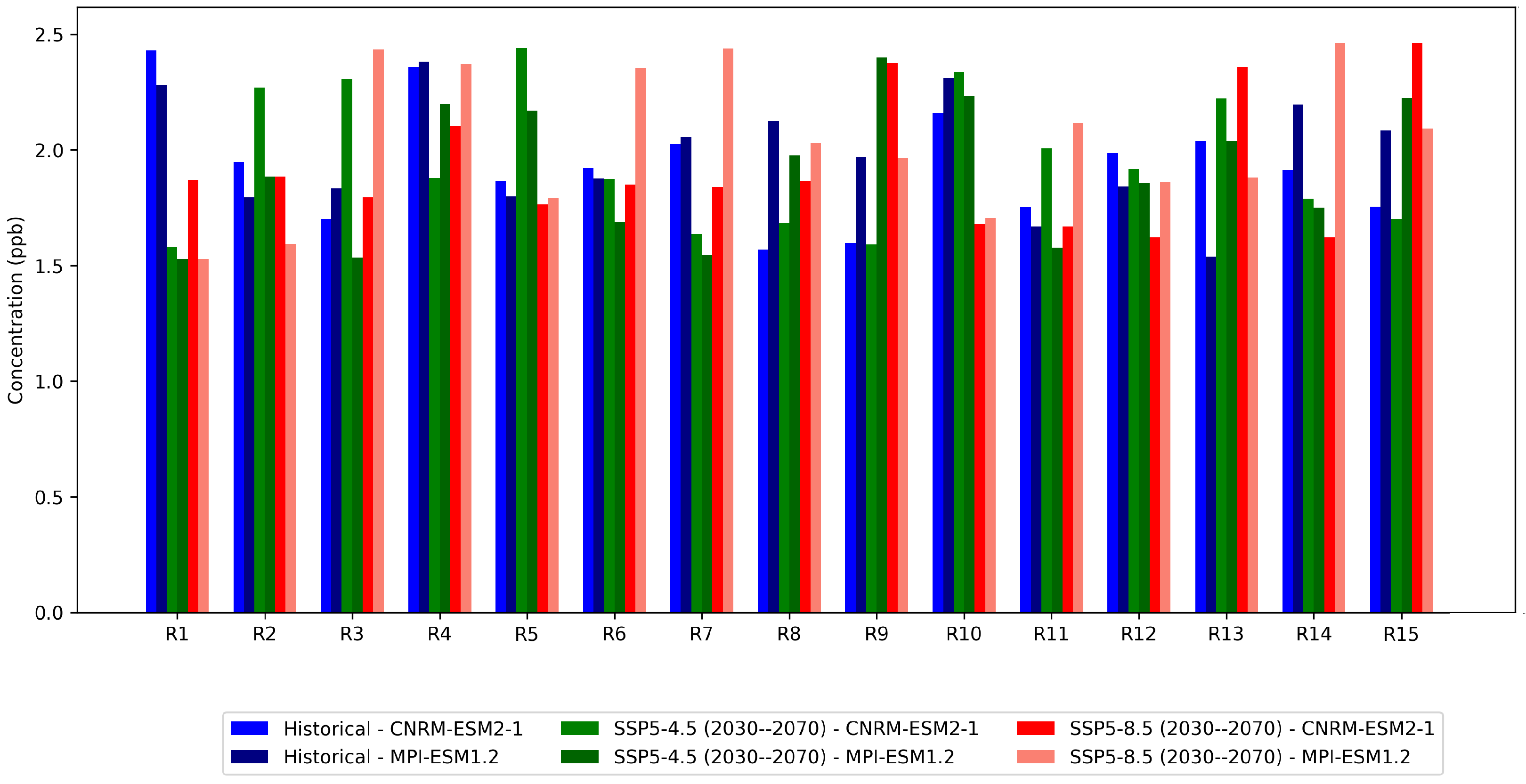
3.2. Spatial Variability of SO₂ Pollution in Future Emission Scenarios

Figure 1 illustrates the historical and projected sulfur dioxide (SO₂) concentrations across 15 districts of Riyadh, based on two distinct climate models, CNRM-ESM2-1 and MPI-ESM1.2, under three scenarios: the historical period (2000–2014), SSP5-4.5 (2030–2070), and SSP5-8.5 (2030–2070). A general increase in SO₂ levels is observed in the projections, particularly under the SSP5-8.5 scenario, for which both models predicted significantly higher concentrations than the historical period. This upward trend is especially pronounced in highly urbanized and high-traffic areas, such as R5 (Al Shifa), R13 (Mecca Road), and R14 (North Ring Road), where the projected concentrations exceed 4.0 ppb under the SSP5-8.5 scenario. Figure 2 presents the average evolution of sulfur dioxide (SO₂) concentrations simulated using the SSP5-4.5 and SSP5-8.5 socio-economic scenarios for the period 2030–2070, compared to the historical period (2000–2015), based on two distinct climate models: CNRM-ESM2-1 and MPI-ESM1.2. A general increase in SO₂ concentrations is observed in the future projections, regardless of the model or scenario considered. This increase is more pronounced under the SSP5-8.5 scenario, which corresponds to a high-emission trajectory, whereas the more moderate SSP5-4.5 scenario shows intermediate results. Moreover, the CNRM-ESM2-1 model tends to simulate slightly higher concentrations than the MPI-ESM1.2 model, indicating a potentially greater sensitivity to climate change. The displayed standard deviations reflect a non-negligible degree of uncertainty, but the overall trends remain consistent, highlighting the growing impact of the emission scenarios on projected air quality.

Regional disparities in SO₂ concentrations can be attributed to several local factors, including intensified industrial activities, traffic density, and geographical features that favor pollutant accumulation. For example, districts R5, R13, and R14 are located in zones with strong commercial and industrial activity, where an increase in SO₂ levels is anticipated. This is likely due to ongoing urban expansion and the development of transportation infrastructure, which exacerbates the degradation of air quality. The MPI-ESM1.2 model tends to predict slightly higher SO₂ levels than the CNRM-ESM2-1 model, particularly in future scenarios. This difference may reflect MPI-ESM1.2’s greater sensitivity to emission pathways and regional climate–pollution interactions. This may also better represent the local pollution processes related to industrial emissions and road traffic. These observations are consistent with previous studies reporting increasing urban air quality deterioration in the Middle East in the absence of robust mitigation policies [53,54].

The increase in SO₂ concentrations under the SSP5-8.5 scenario, a high-emission trajectory, reflects the continued reliance on fossil fuels and limited mitigation efforts. This finding aligns with the Intergovernmental Panel on Climate Change (IPCC) Sixth Assessment Report [1] and other regional studies [55] that emphasize the significant impact of industrial emissions in Saudi Arabia and highlight the urgency of strengthening air quality management.

These results underscore the importance of implementing targeted emission control strategies, particularly in industrial zones and areas with high traffic densities. Policies promoting the modernization of transport systems, the adoption of emission reduction technologies, and the transition to cleaner energy sources are essential to mitigate SO₂ pollution and its associated health and environmental risks. Immediate and sustained action is crucial to preserve air quality and public health in Riyadh, according to international recommendations for managing air pollution in rapidly urbanizing regions. A Bayesian statistical analysis of sulfur dioxide (SO₂) concentrations highlighted a trend of increasing average levels in the future projections compared to the historical period (2000–2015). The estimated means (${\mu }_{\mathrm{scenario}}$) ranged from 2.22 to 2.31 during the historical period and reached higher levels, up to 2.81, under the SSP5-8.5 scenario (

Table 2. Estimated mean SO₂ concentrations (${\mu }_{\mathrm{scenario}}$) and standard deviations (SDs) under historical and future climate scenarios from two climate models.

Scenario	Mean (${\mathit{\mu }}_{\mathbf{scenario}}$)	SD	HDI 2.5%	HDI 97.5%
Historical—CNRM-ESM2-1	0.039	0.248	−0.571	0.393
Historical—MPI-ESM1.2	0.049	0.233	−0.462	0.446
SSP5-4.5—CNRM-ESM2-1	0.042	0.240	−0.484	0.406
SSP5-4.5—MPI-ESM1.2	−0.098	0.276	−0.407	0.470
SSP5-8.5—CNRM-ESM2-1	−0.023	0.238	−0.371	0.602
SSP5-8.5—MPI-ESM1.2	0.135	0.259	−0.349	0.529

). This evolution suggests a possible increase in atmospheric SO₂ concentrations linked to the combined effects of climate change and emissions. This increase can be explained by the complex interactions among climate change, anthropogenic emissions, and atmospheric processes that influence both the dispersion and chemical transformation of SO₂. The observed moderate variability (global standard deviation $\sigma \approx 0.14$) indicates the relative stability of the results, despite the uncertainties inherent in the climate models used. Furthermore, the convergence diagnostics of the Bayesian chains confirmed the robustness of the estimates.

These results align with those of previous studies, such as those by Langner et al. [56] and Ward [57], which demonstrated the significant impact of climate change on atmospheric sulfur pollutants, notably through changes in precipitation patterns and temperatures that affect the chemical conversion and transport of SO₂. These observations underscore the importance of integrating climate projections into air quality management strategies to anticipate the long-term effects of climate change on atmospheric pollution and on public health.

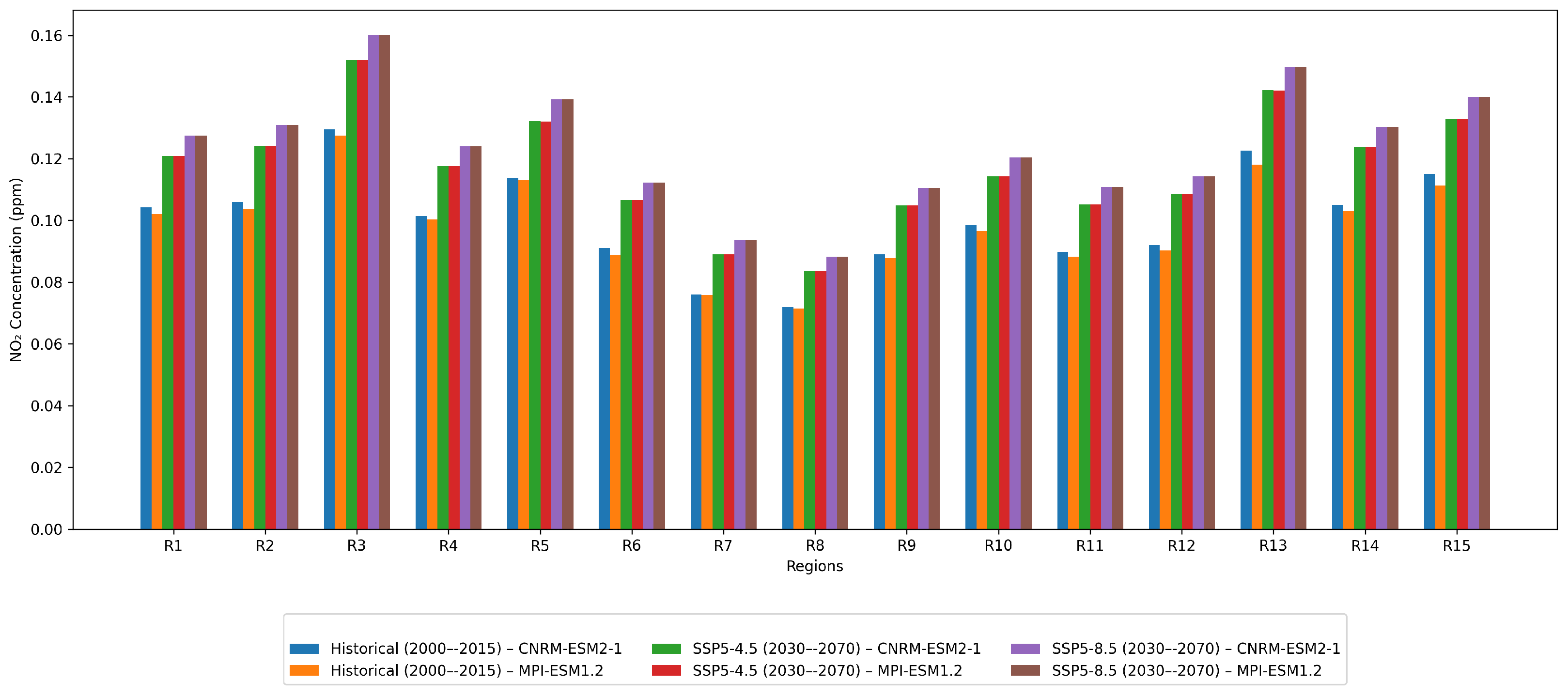
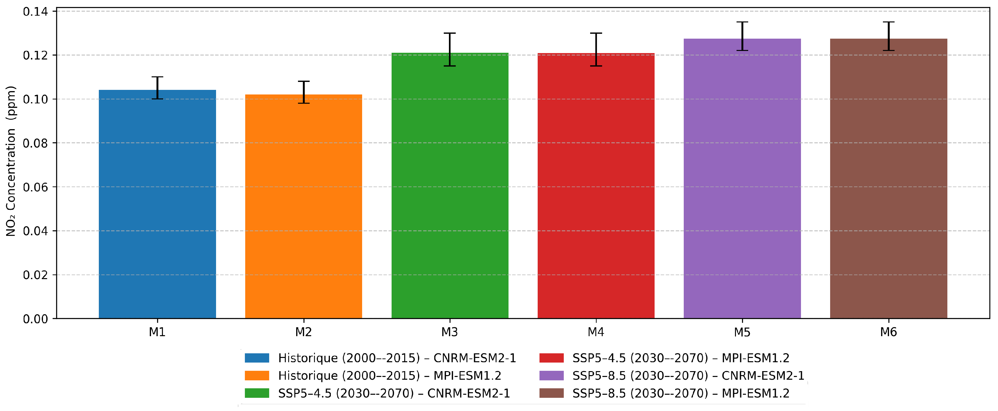
3.3. Spatial Variability of NO₂ Pollution in Future Emission Scenarios

Regional nitrogen dioxide NO₂ concentrations simulated by the CMIP6 models (CNRM-ESM2-1 and MPI-ESM1.2) indicate a widespread increase in the future projections (2030–2070) compared to the historical reference period (2000–2015) under both emission scenarios: SSP5-4.5 and SSP5-8.5 (Figure 3). This increase is more pronounced under the SSP5-8.5 scenario, reflecting the exacerbating effect of a high-carbon-intensity socio-economic development pathway [7].

For instance, in region R3, the average NO₂ concentration rises from approximately 0.129 ppm (historical, CNRM-ESM2-1) to 0.160 ppm (SSP5-8.5, CNRM-ESM2-1), representing an increase of about 24%. Similarly, region R13 experiences an increase from 0.123 ppm to 0.149 ppm over the same period and scenario, equating to an approximate 21% rise (Figure 3). These increases reflect a general trend toward intensified NO₂ pollution, particularly in densely populated and industrialized regions.

However, notable spatial variations are observed across regions. Regions R3, R5, R13, and R15 consistently exhibit the highest levels, both historically and in future projections. Conversely, areas such as R8 and R7 display the lowest concentrations (e.g., R8 increased from 0.072 ppm to 0.088 ppm), which may be attributed to lower urbanization or emission densities (Figure 3). These inter-regional contrasts underscore the importance of incorporating spatial dimensions into mitigation policies.

The hierarchical Bayesian analysis (

Table 3. Estimated mean NO₂ concentrations (${\mu }_{\mathrm{scenario}}$) and standard deviations (SDs) under historical and future climate scenarios from two climate models.

Scenario (Index)	Mean (${\mathit{\mu }}_{\mathbf{scenario}}$)	SD	HDI 2.5%	HDI 97.5%
Historical—CNRM-ESM2-1	0.011	0.289	−0.547	0.551
Historical—MPI-ESM1.2	−0.004	0.290	−0.597	0.571
SSP5-4.5—CNRM-ESM2-1	0.007	0.293	−0.572	0.549
SSP5-4.5—MPI-ESM1.2	0.011	0.288	−0.572	0.521
SSP5-8.5—CNRM-ESM2-1	0.014	0.287	−0.577	0.542
SSP5-8.5—MPI-ESM1.2	0.010	0.292	−0.587	0.548

) applied to the different climate model– scenario combinations highlight moderate but significant variations in the estimated mean SO₂ concentrations (${\mu }_{scenario}$). Under the SSP5-8.5 scenario, the results indicate a more pronounced increase in average levels, especially with the MPI-ESM1.2 model ($\mu =0.135$) and, to a lesser extent, with CNRM-ESM2-1 ($\mu =-0.023$). Wide credible intervals reflect considerable uncertainty. This trend, illustrated in Figure 4, suggests that high-emission scenarios may intensify future SO₂ concentrations, particularly in arid regions such as Riyadh, which are already exposed to extreme climatic conditions. Previous studies [58,59] have shown that the specific meteorological features of this region, namely, intense heat, low humidity, and limited wind, favor the stagnation and accumulation of air pollutants. Moreover, Jacob and Winner [60] and Fiore et al. [61] emphasized the indirect effects of climate change on air quality by altering atmospheric transport and chemical transformation processes. The higher sensitivity observed with the MPI-ESM1.2 model likely reflects an amplified response to radiative forcing, consistent with the findings of Tebaldi and Knutti [62] regarding inter-model variability. Although additional adjustments are needed to improve MCMC chain convergence (with some $\widehat{R}$ values exceeding 1.1), these results support the hypothesis that climate change will exacerbate regional air pollution levels, necessitating the development of targeted mitigation strategies.

3.4. Projected Temporal Evolution of NO₂ Concentrations

Figure 5 presents the temporal evolution of NO₂ concentrations from 2030 to 2070 across several representative zones of Riyadh, based on two climate models (CNRM and MPI) combined with two contrasting socio-economic scenarios (SSP2-4.5 and SSP5-8.5). A progressive and pronounced increase in concentrations is observed in all studied zones, particularly under the MPI model with the SSP5-8.5 scenario. The most affected areas include major traffic corridors (R11, R14, R15) and densely urbanized zones (R12, R13), where concentrations exceed 100 μg m⁻³ by 2070—well above the annual limit recommended by the World Health Organization (40 μg m⁻³) [2]. These results reflect the combined effects of intensified anthropogenic activities, rapid urbanization, and increased emissions from road transport in the context of unfavorable climate change [63,64]. Increases are also recorded in semi-natural areas (R2 and R3), indicating regional diffusion of pollutants.

The discrepancy between the two climate models, particularly the overestimation by MPI under SSP5-8.5, may be attributed to a greater sensitivity to climatic feedbacks in arid environments [65]. These trends highlight the urgent need for emission reduction policies, particularly in the transport and energy sectors, to safeguard air quality and public health in urban settings [66].

3.5. Projected Temporal Evolution of SO₂ Concentrations

Temporal projections of SO₂ concentrations between 2030 and 2070 reveal marked spatial stratification, with significantly higher levels in urbanized areas (R12, R13) and transport corridors (R11, R14, R15) than in semi-natural zones (R2, R3), consistent with urban–rural gradient observations documented in the literature [67,68] (Figure 6). A comparative analysis of the SSP2-4.5 and SSP5-8.5 scenarios highlights the nonlinear amplification of pollution under the high-emission scenario, with concentrations potentially exceeding 70 μg m⁻³ by 2070, representing 2–3 times the WHO-recommended thresholds [2,69].

The divergence between the CNRM and MPI models, particularly pronounced under SSP5-8.5, suggests the differential sensitivity of climate parameterizations to arid conditions [65,70], with the MPI model exhibiting a more pronounced response to anthropogenic forcing in accordance with regional-model intercomparison studies [71,72]. The generalized increase in concentrations, including in peri-urban areas, indicates long-range transport effects and regional background pollution [64,73], highlighting the need for integrated mitigation approaches at the metropolitan scale to limit the future exposure of the Riyadh population to atmospheric pollutants [66,74].

3.6. Spatial and Temporal Variability of PM_2.5 and O₃ Pollution in Future Emission Scenarios

Climate projections for the period 2030–2070 reveal a marked increase in tropospheric ozone (O₃) and fine particulate matter (PM_2.5) concentrations across the Riyadh region [27]. This trend, particularly pronounced under the high-emission scenario SSP5-8.5 [75], was observed in both the CNRM [76] and MPI [77] climate models. This deterioration results from the combined effects of climate change, intensified anthropogenic activities, and rapid urban expansion [29].

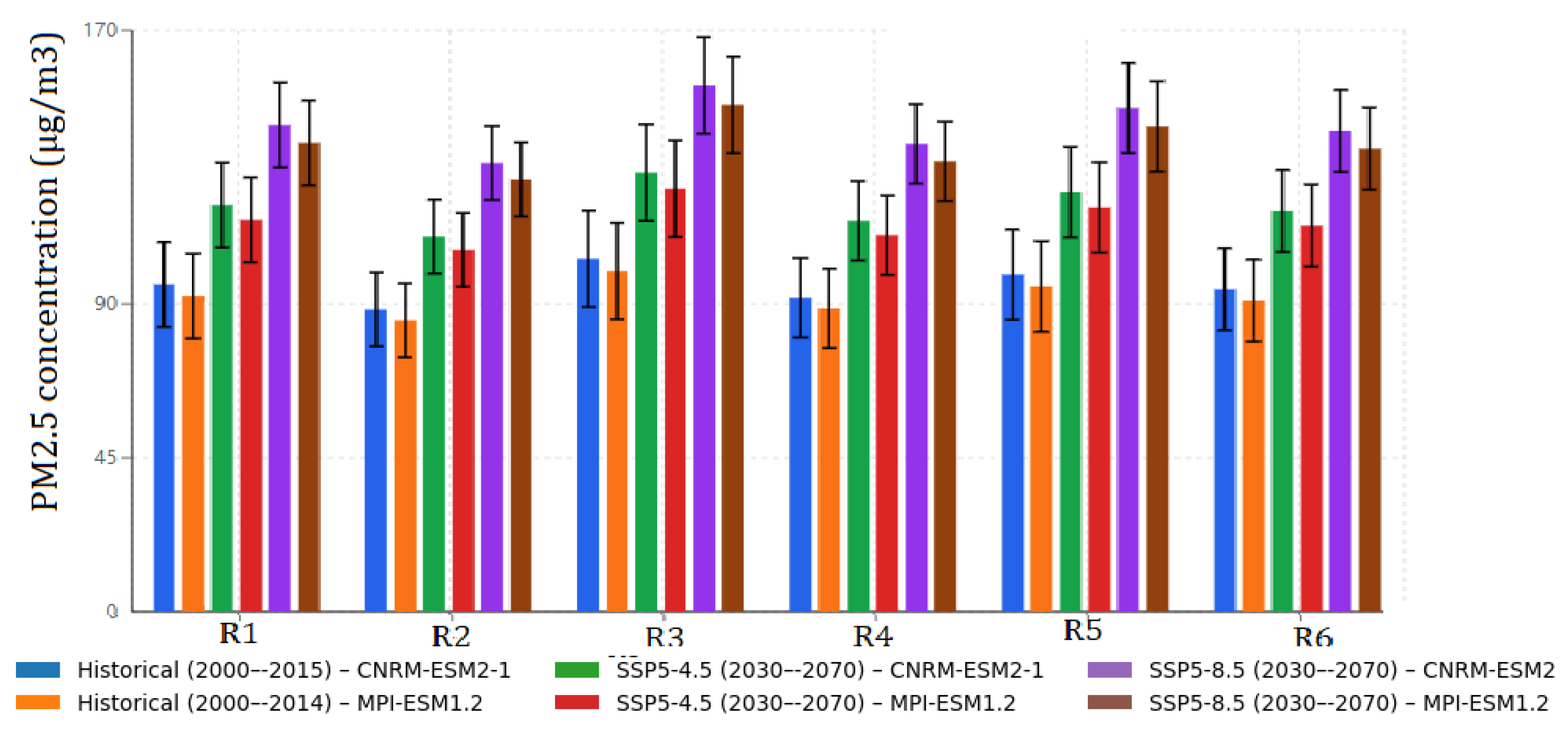
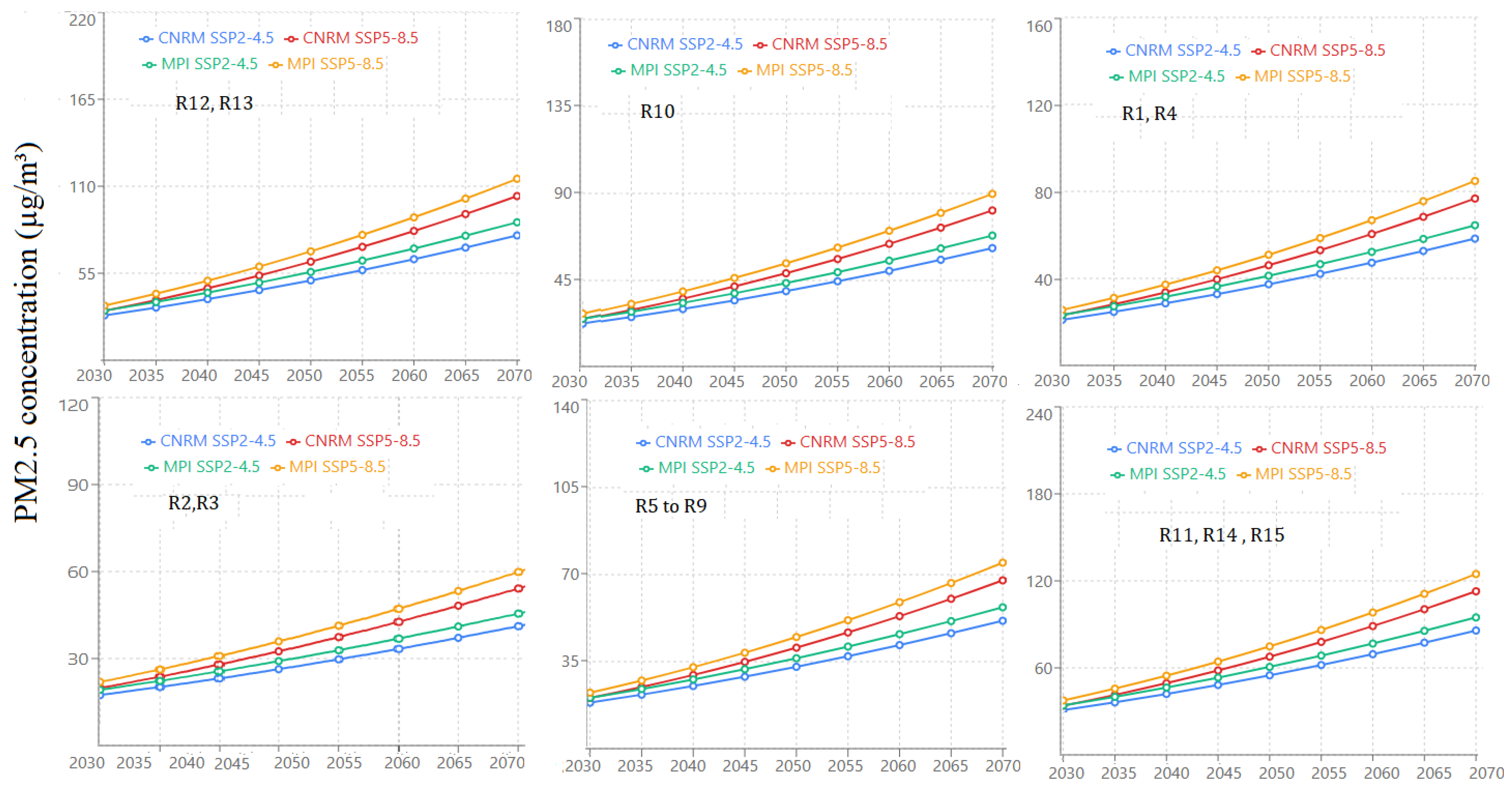
3.6.1. PM_2.5 Concentration Analysis

A comparison between the historical and projected PM_2.5 concentrations reveals significant temporal and spatial variations across the study domain (Figure 7). Historical data (2000–2014) from both the CNRM-ESM2-1 and MPI-ESM1.2 models show relatively uniform concentrations across regions R1–R6, with values ranging from 35 to 50 μg/m³. The CNRM-ESM2-1 model indicates slightly higher historical concentrations (40–48 μg/m³) compared to MPI-ESM1.2 (35–45 μg/m³), with R3 showing the highest historical values in both models.

The comprehensive statistical analysis of PM_2.5 concentrations across all regional models reveals distinct patterns between climate scenarios and models (

Table 4. Estimated mean PM_2.5 concentrations (${\mu }_{\mathrm{scenario}}$) and standard deviations (SDs) under historical and future climate scenarios from two climate models.

Scenario (Model)	Mean (${\mathit{\mu }}_{\mathbf{scenario}}$)	SD	Min	Max
Historical—CNRM-ESM2-1	45.13	4.25	38.9	52.6
Historical—MPI-ESM1.2	42.53	4.89	36.4	49.8
SSP2-4.5—CNRM-ESM2-1	58.90	5.68	51.2	67.4
SSP2-4.5—MPI-ESM1.2	55.97	5.37	48.7	64.1
SSP5-8.5—CNRM-ESM2-1	73.33	7.14	64.8	83.7
SSP5-8.5—MPI-ESM1.2	69.97	6.63	61.9	79.9

). Under the SSP2-4.5 moderate-emission scenario (2030–2070), both models project substantial increases, albeit with notable differences. The CNRM-ESM2-1 model projects concentrations of 50–62 μg/m³ across regions, with R3 reaching the highest values (∼62 μg/m³), followed by R1 and R5 (∼58 μg/m³). In contrast, the MPI-ESM1.2 model shows more conservative projections (48–58 μg/m³), with R3 again showing peak concentrations. Regions R2, R4, and R6 consistently show lower concentrations in both models under this scenario.

The SSP5-8.5 high-emission scenario reveals the most severe deterioration, with marked differences between models and regions. The CNRM-ESM2-1 model projects concentrations reaching 60–68 μg/m³, with R3 and R5 showing the highest values (∼68 μg/m³ and ∼65 μg/m³, respectively). The MPI-ESM1.2 model projects slightly lower but still critical concentrations (58–65 μg/m³), maintaining R3 as the most polluted region (∼65 μg/m³). When compared to historical data, this represents an increase of 35–70% depending on the region and model, as evidenced by the mean concentrations presented in Table 4.

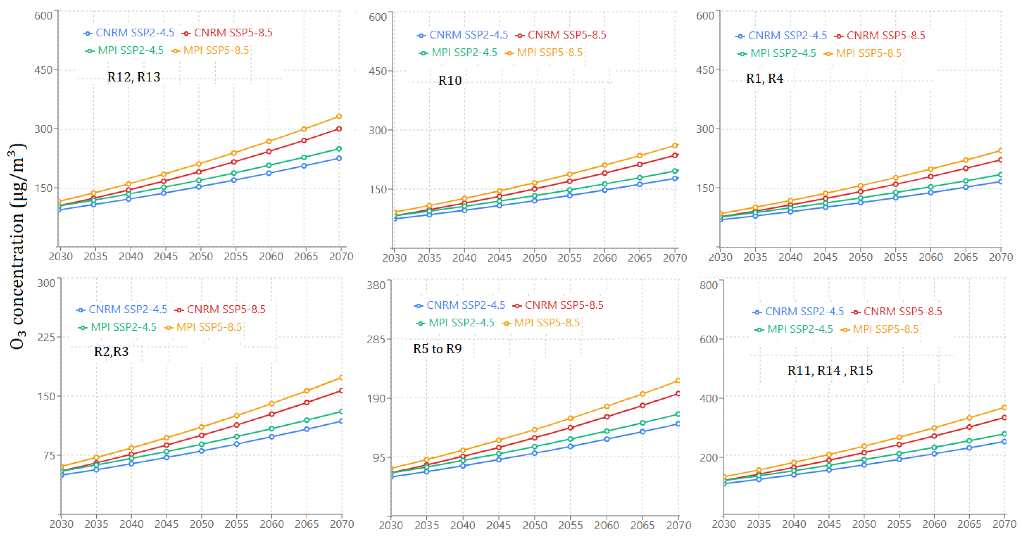
3.6.2. O₃ Concentration Projections

Ozone concentrations show even more dramatic increases across all scenarios and models (Figure 8). Historical concentrations (2000–2015) were relatively uniform across regions R1–R6, with both models indicating concentrations between 85 and 95 μg/m³. The CNRM-ESM2-1 model shows slightly higher historical values (88–95 μg/m³) compared to MPI-ESM1.2 (85–92 μg/m³), with minimal spatial variation.

The statistical summary of O₃ concentrations demonstrates the severity of future ozone pollution across all scenarios (

Table 5. Estimated mean O₃ concentrations (${\mu }_{\mathrm{scenario}}$) and standard deviations (SDs) under historical and future climate scenarios from two climate models.

Scenario (Model)	Mean (${\mathit{\mu }}_{\mathbf{scenario}}$)	SD	Min	Max
Historical—CNRM-ESM2-1	95.33	5.65	88.4	103.2
Historical—MPI-ESM1.2	91.98	5.50	85.2	99.6
SSP2-4.5—CNRM-ESM2-1	118.53	6.92	109.7	128.4
SSP2-4.5—MPI-ESM1.2	114.22	6.63	105.8	123.7
SSP5-8.5—CNRM-ESM2-1	142.02	8.64	131.2	153.9
SSP5-8.5—MPI-ESM1.2	136.78	8.21	126.4	148.2

). Under the SSP2-4.5 scenario, significant increases are observed with clear spatial differentiation. The CNRM-ESM2-1 model projects concentrations of 95–115 μg/m³, with R3 and R5 showing the highest values (∼115 μg/m³ and ∼112 μg/m³, respectively). The MPI-ESM1.2 model indicates similar spatial patterns but with slightly lower absolute values (92–110 μg/m³). Regions R1, R2, R4, and R6 maintain more moderate concentrations (95–105 μg/m³) in both models.

The SSP5-8.5 scenario projects critical ozone levels across all regions. The CNRM-ESM2-1 model indicates concentrations reaching 125–142 μg/m³, with R3 showing the most severe pollution (∼142 μg/m³), followed closely by R5 (∼138 μg/m³). The MPI-ESM1.2 model projects similarly alarming levels (120–138 μg/m³), maintaining the same spatial pattern. Compared to historical data, these projections represent increases of 40–60% across all regions, as summarized in the statistical analysis presented in Table 5.

3.6.3. Model–Scenario Regional Comparisons

The comparative analysis reveals consistent patterns across both climate models, despite the quantitative differences. The CNRM-ESM2-1 model systematically projects higher concentrations for both pollutants compared to MPI-ESM1.2, with differences ranging from 2 to 8 μg/m³ for PM_2.5 and 3 to 10 μg/m³ for O₃. However, both models agree on the spatial ranking of regions, with R3 consistently emerging as the most polluted region under all scenarios.

The scenario comparison shows that the SSP5-8.5 projections exceed the SSP2-4.5 values by 8–15 μg/m³ for PM_2.5 and 15–25 μg/m³ for O₃ across all regions and models. This demonstrates the critical importance of emission pathway selection for future air quality outcomes, as clearly illustrated by the mean concentration differences between scenarios in Table 4 and Table 5.

The regional analysis reveals that R3 and R5 consistently show the highest pollution levels under future scenarios, whereas R2, R4, and R6 maintain relatively lower concentrations. R1 exhibits intermediate pollution levels across all scenarios. This spatial pattern suggests that urban development and industrial activities will concentrate in specific areas, creating distinct pollution gradients across metropolitan regions.

3.6.4. Health and Environmental Implications

These projected concentrations have severe health implications when compared with the WHO guidelines [78]. For PM_2.5, future concentrations will exceed the WHO annual guideline (5 μg/m³) by factors of 10–14 under SSP2-4.5 and 12–16 under SSP5-8.5. Even the WHO interim target (15 μg/m³) will be surpassed by factors of 3–4.5 across all regions and scenarios.

For ozone, the projected concentrations substantially exceed the WHO 8 h guideline (100 μg/m³) under both scenarios, with exceedances of 10–42 μg/m³ depending on the region and scenario. The WHO annual guideline for ozone (60 μg/m³) will be exceeded by factors of 1.6–2.4 across all projections, indicating widespread health risks for the population.

3.6.5. Temporal Evolution and Regional Hotspots

The temporal evolution analysis reveals distinct patterns of pollution development across different regional clusters (Figure 9 and Figure 10). The integration of temporal data from the comprehensive time-series analysis provides critical insights into the progression of air pollution across the Riyadh metropolitan region.

PM_2.5 Temporal Trajectories

The temporal analysis of PM_2.5 concentrations across different regional clusters reveals alarming upward trends, with distinct patterns for each geographical zone. The highly urbanized core regions (R11, R14, R15) demonstrate the most critical pollution trajectory, with concentrations projected to increase from baseline levels of 45–50 μg/m³ in 2030 to 90–130 μg/m³ by 2070 under SSP5-8.5. This represents a doubling of concentrations over the 40-year period, with a consistent annual increase rate of 1.5–2 μg/m³ per year.

The industrial and commercial zones (R12, R13) exhibit similarly concerning trends, with concentrations rising from initial values of 40–45 μg/m³ in 2030 to 85–110 μg/m³ by 2070. These regions show a linear growth pattern with noticeable acceleration after 2050, suggesting the compounding effects of industrial expansion and climate change impacts.

The central urban area (R10) displays intermediate pollution levels, with concentrations increasing from 35–40 μg/m³ in 2030 to 75–90 μg/m³ by 2070. This region maintains a steady but moderate growth rate throughout the projection period.

Peripheral regions show varied patterns: R1 and R4 maintain the lowest absolute concentrations but still experience significant increases from 30–35 μg/m³ to 65–85 μg/m³. Regions R2, R3, and R5–R9 follow intermediate trajectories, with concentrations rising from 20–30 μg/m³ in 2030 to 45–70 μg/m³ by 2070.

O₃ Temporal Evolution

The ozone concentration projections reveal even more dramatic temporal changes, with critical implications for public health. The highly urbanized core regions (R11, R14, R15) emerge as extreme pollution hotspots, with concentrations projected to increase from baseline levels of 150–160 μg/m³ in 2030 to 350–450 μg/m³ by 2070 under SSP5-8.5. This represents a 2.5-to-3-fold increase, with the steepest temporal gradients showing annual increases of 5–7 μg/m³ throughout the projection period.

The industrial and commercial zones (R12, R13) display similarly alarming trends, with ozone concentrations rising from 100–110 μg/m³ in 2030 to 250–350 μg/m³ by 2070. Notably, the MPI-ESM1.2 model consistently projects higher concentrations in these regions compared to CNRM-ESM2-1, with differences reaching 20–30 μg/m³ by 2070.

The central urban area (R10) shows intermediate but still critical pollution levels, with concentrations increasing from 85–95 μg/m³ in 2030 to 200–250 μg/m³ by 2070. This region maintains a consistent upward trajectory throughout the projection period.

Peripheral regions (R1, R4, R2, R3, and R5–R9) demonstrate more moderate but still significant increases. R1 and R4 show concentrations rising from 80–90 μg/m³ to 180–220 μg/m³, while R2, R3 increase from 60–75 μg/m³ to 140–180 μg/m³, and R5–R9 rise from 70–85 μg/m³ to 160–200 μg/m³ by 2070.

Inter-Scenario Temporal Comparison

The comparative analysis between SSP2-4.5 and SSP5-8.5 scenarios reveals increasingly divergent trajectories over time. For PM_2.5, the difference between scenarios grows from 10–15 μg/m³ in 2030 to 20–30 μg/m³ by 2070, representing a 25–35% higher concentration under the high-emission scenario. This divergence becomes more pronounced in the latter half of the projection period, emphasizing the long-term consequences of emission pathway choices.

For ozone, the scenario differences are even more dramatic, with gaps widening from 15–25 μg/m³ in 2030 to 40–60 μg/m³ by 2070. The SSP5-8.5 scenario consistently produces concentrations 30–40% higher than SSP2-4.5 across all regional clusters.

Model Agreement and Uncertainty

The temporal analysis confirms that both the CNRM-ESM2-1 and MPI-ESM1.2 models consistently identify the same regional hierarchy in terms of pollution severity, with the highly urbanized core areas (R11, R14, and R15) representing the most critical pollution hotspots. However, notable inter-model differences emerges in the temporal trajectories: the MPI model tends to project 10–20% higher concentrations for ozone, particularly in industrial zones, while CNRM shows slightly higher PM_2.5 projections in urban areas.

Despite these quantitative differences, the qualitative agreement between the models reinforces the robustness of the overall trends and the identification of critical pollution hotspots. Both models consistently show accelerating pollution trends after 2050, suggesting that the combined effects of climate change and urban development will intensify air quality deterioration in the latter half of the projection period.

For ozone concentrations, the most critical situation emerges in the highly urbanized core regions (R11, R14, R15), where concentrations are projected to increase from baseline levels of 150 μg/m³ in 2030 to 350–450 μg/m³ by 2070 under SSP5-8.5. These regions consistently show the steepest temporal gradients, with annual increases of 5–7 μg/m³ throughout the projection period.

The industrial/commercial zones (R12, R13) display similarly alarming trends, with ozone concentrations rising from 100 μg/m³ in 2030 to 250–350 μg/m³ by 2070. The MPI-ESM1.2 model consistently projects higher concentrations in these regions than CNRM-ESM2-1, with differences reaching 20–30 μg/m³ by 2070.

Peripheral regions (R2, R3, and R5–R9) show more moderate but still significant increases, with concentrations rising from 60–90 μg/m³ in 2030 to 140–200 μg/m³ by 2070 under SSP5-8.5. The central urban area (R10) displayed intermediate pollution levels, with concentrations reaching 200–250 μg/m³ by 2070.

For PM_2.5, the temporal patterns reveal a more uniform but equally concerning trend across all regional clusters. The highly urbanized regions (R11, R14, R15) show concentrations increasing from 45–50 μg/m³ in 2030 to 90–130 μg/m³ by 2070 under SSP5-8.5, representing the most severe PM_2.5 pollution in the study area.

The industrial zones (R12, R13) and central area (R10) display similar trajectories, with concentrations rising from initial values of 35–45 μg/m³ to 80–110 μg/m³ by 2070. Peripheral regions (R2, R3, R5–R9) maintain relatively lower but still critical levels, increasing from 20–30 μg/m³ in 2030 to 45–70 μg/m³ by 2070.

A comparative analysis between the SSP2-4.5 and SSP5-8.5 scenarios reveals that the high-emission pathway consistently produces 15–25% higher concentrations of both pollutants across all regions. This difference becomes more pronounced toward the end of the projection period, emphasizing the long-term consequences of the emission pathway choices.

The model agreement analysis showed that both CNRM-ESM2-1 and MPI-ESM1.2 consistently identified the same regional hierarchy in terms of pollution severity, with the highly urbanized core areas (R11, R14, and R15) representing the most critical pollution hotspots. However, the MPI model tended to project 10–20% higher concentrations for ozone, while CNRM showed slightly higher PM_2.5 projections.

This comprehensive analysis demonstrates that regardless of the climate model or emission scenario considered, air quality in the Riyadh region will deteriorate significantly, with some areas experiencing particularly severe pollution levels that pose substantial health risks to the population.

4. Discussion

The projections from this study confirmed a significant degradation of air quality in Riyadh, particularly under the SSP5-8.5 scenario. This trend is consistent with the 2024 World Air Quality Report, which indicates that only 17% of cities comply with WHO standards [79]. The anticipated increases in NO₂ (45–55%) and SO₂ (80–130%) concentrations far exceed recommended health thresholds [2], raising fundamental questions about the viability of the current urban development model in arid zones.

The spatial distribution of pollutants highlights higher concentrations along transport corridors (R11, R14, R15) and in densely populated urban areas (R12, R13), revealing the direct impact of road traffic and industrial activities [80,81]. This pattern aligns with observations made in other arid cities in the Middle East, where extreme climatic conditions exacerbate pollutant accumulation [82,83].

The differences observed between the CNRM-ESM2-1 and MPI-ESM1.2 models under the SSP5-8.5 scenario illustrate the inherent inter-model variability in short-term climate projections [84,85]. These differences, especially those pronounced for atmospheric pollutant concentrations, reflect variations in physico-chemical parameterization schemes and the representation of climate–atmosphere interactions. These aspects are particularly critical in arid environments, where pollutant dispersion and transformation processes are intensified [86].

The increased sensitivity of the MPI-ESM1.2 model to anthropogenic forcings can be attributed to its specific treatment of convection and vertical mixing processes, which directly influence the vertical distribution of pollutants in the atmosphere boundary layer. This inter-model variability constitutes a realistic estimate of structural uncertainty in climate projections [87].

The lack of recent data, notably post-2015, limits the ability to validate and adjust model outputs based on the actual atmospheric conditions observed in Riyadh in the context of rapid urbanization and evolving emission sources [79]. To overcome this limitation, rigorous bias correction methods were applied in line with the best practices in climate modeling [60,88]. These corrections adjust model outputs by accounting for discrepancies identified between historical simulations and available observations (2000–2015), thereby reducing uncertainties related to physico-chemical parameterizations and anthropogenic forcings. The adopted probabilistic approach, including hierarchical credibility intervals, explicitly quantifies residual uncertainty while preserving the robustness of the projected trends. Although the lack of recent validation data may limit the fine-tuning of the models, the bias correction procedures ensure that projections remain consistent with the dominant atmospheric mechanisms in arid environments [86]. This methodology, combined with inter-model agreement on significant air quality degradation, strengthens the reliability of the conclusions for adaptation policy development.

The hierarchical Bayesian analysis applied in this study enables rigorous quantification of this uncertainty by integrating both inter-model variability and parametric uncertainty. The resulting credibility intervals reflect the current state of scientific knowledge and provide a robust tool for risk assessment [89,90]. This probabilistic approach aligns with the IPCC recommendations for regional climate projection assessments [88].

Despite these uncertainties, all models converge toward a consistent signal of significant air quality deterioration by 2070. This robustness, regardless of modeling differences, strengthens confidence in the identified trends and underscores the need to promptly implement preventive adaptation measures [60].

The results indicate a pronounced and spatially uneven degradation of air quality in Riyadh between 2030 and 2070, especially under SSP5-8.5. Historical PM_2.5 levels already exceeded WHO guidelines by a factor of 7–10, and are projected to rise by an additional 35–70%, with concentrations reaching 70–83 μg/m³ in urban and industrial zones such as R3, R5, R11, R14, and R15. Ozone (O₃) is expected to follow a similar trajectory, exceeding 140 μg/m³ under SSP5-8.5—40–60% above current levels and well beyond the WHO 8-hour guideline. The divergence between SSP2-4.5 and SSP5-8.5 becomes particularly stark after 2050. The CNRM-ESM2-1 and MPI-ESM1.2 models show consistent spatial and temporal patterns despite a 10–20% difference in magnitude, with CNRM projecting higher PM_2.5 and MPI higher ozone. These levels pose serious health risks, particularly to vulnerable populations, and call for targeted mitigation, air quality monitoring, and integrated air–climate strategies.

Projected NO₂ concentrations exceeding 100 μg/m³ in certain urban zones pose a major health risk, especially for vulnerable populations. Chronic exposure to such levels is strongly linked to increased morbidity and mortality from respiratory and cardiovascular diseases [91,92]. This finding echoes concerns raised in the United Nations Declaration on the Right to Clean Air [93].

These health impacts also entail considerable economic costs, including healthcare expenditures, reduced productivity, and diminished quality of life [94]. Yet, only 3% of companies currently report pollutant emission reduction actions [95], highlighting the urgent need for stricter regulations and effective incentive mechanisms.

The observed trends in Riyadh align with those documented in other major arid cities of the Middle East and North Africa [96,97]. However, several international examples demonstrate that a change in trajectory is possible. Cities that have implemented ambitious air quality policies have recorded significant improvements [98,99,100]. These experiences show that political commitment, coupled with targeted investments in clean technologies and sustainable urban planning, can reverse negative trends.

The results of this study thus call for a swift and structured political response. Given the inertia of the climate system and the persistence of pollutants in the atmosphere, decisions made today will shape urban living conditions for decades to come [101]. Priorities must include vehicle fleet modernization, development of public transportation, improved energy efficiency of buildings, and increased use of clean energy sources [102]. These measures offer dual benefits: improving local air quality and contributing to greenhouse gas emission reductions, in line with international recommendations [103].

Several research avenues deserve further exploration. Integration of satellite data represents a major advance for spatial validation of projections and precise identification of emission sources [104,105]. Developing coupled models incorporating meteorological, chemical, and socio-economic dimensions is essential to refine long-term projections [106]. In this context, artificial intelligence appears as a particularly promising tool to manage the growing complexity of these systems [107].

Finally, detailed economic evaluation of mitigation strategies, including health and climate benefits, would strengthen the relevance of policy choices, especially in resource-limited settings [108,109].

5. Conclusions

This study provides strong evidence of substantial air quality deterioration in Riyadh under future climate scenarios, with projected increases in SO₂ (80–130%) and NO₂ (45–55%) concentrations far exceeding WHO guidelines by 2070. By integrating CMIP6 climate models with a hierarchical Bayesian analysis applied across 15 monitoring stations, our findings reveal consistent degradation trends despite inter-model variability, particularly under the high-emission SSP5-8.5 scenario.

Spatial analysis revealed marked pollution gradients, with traffic corridors (stations R11, R14, and R15) and densely urbanized areas (stations R12 and R13) experiencing the most severe increases, while pollutant transport between stations also affected semi-natural zones.

The 95% Bayesian credible intervals for the projected mean SO₂ concentrations under the SSP5-8.5 scenario ranged from −0.37 to +0.60 ppb for the CNRM-ESM2-1 model and from −0.35 to +0.53 ppb for the MPI-ESM1.2 model. For NO₂, the intervals extended from −0.58 to +0.54 ppb, while inter-model differences reached up to 0.16 ppb for SO₂ and 0.02 ppb for NO₂, highlighting the structural uncertainty inherent in the diversity of climate models used. Sensitivity analyses indicated that variations in the prior distributions and model parameters resulted in less than an 8% change in the posterior means. Despite these uncertainties, the identification of high-risk zones (R3, R5, R11, R14, and R15) remained robust in over 95% of cases, and the high probabilities of exceeding WHO thresholds (ranging from 80% to 98%) reinforced the reliability of the observed trends. Overall, the general trends and spatial distribution of risks appear statistically sound and offer a reliable foundation for informing public policies and developing targeted mitigation strategies.

These results highlight the urgent need for comprehensive emission reduction strategies targeting the transportation and industrial sectors, an accelerated transition to renewable energy, and urban planning reforms that prioritize air quality.

The methodological framework developed in this study provides a valuable reference for similar assessments in other rapidly growing arid cities in the Middle East and North Africa. Future research should incorporate satellite monitoring data, develop coupled socio-economic and environmental models, and assess concrete intervention scenarios to support the implementation of evidence-based policies.

Given the inertia of climate and urban systems, immediate action is essential to prevent projected deterioration and ensure sustainable urban development in one of the world’s most climatically challenging environments.

References

1. Intergovernmental Panel on Climate Change (IPCC). Sixth Assessment Report: Climate Change 2021—The Physical Science Basis; IPCC: Paris, France, 2021. [Google Scholar]
2. WHO. Ambient Air Pollution: Health Impacts; WHO: Geneva, Switzerland, 2021. [Google Scholar]
3. Jacobson, M.Z. Co-benefits of mitigating global greenhouse gas emissions for future air quality and human health. Environ. Sci. Technol. 2012, 46, 4198–4207. [Google Scholar] [CrossRef]
4. Markandya, A.; Sampedro, J.; Smith, S.J.; Dingenen, R.V.; Pizarro-Irizar, C.; Arto, P.I.; González-Eguino, M. Health co-benefits from air pollution and mitigation policies. Lancet Planet. Health 2018, 2, e126–e133. [Google Scholar] [CrossRef] [PubMed]
5. Rao, S.; Klimont, Z.; Leitao, J.; Riahi, K.; van Dingenen, R.; Reis, L.A.; Calvin, K.; Dentener, F.; Drouet, L.; Fujimori, S.; et al. A multi-model assessment of the co-benefits of climate mitigation for global air quality. Environ. Res. Lett. 2016, 11, 124013. [Google Scholar] [CrossRef]
6. O’Neill, B.C.; Kriegler, E.; Riahi, K.; Ebi, K.L.; Hallegatte, S.; Carter, T.R.; Mathur, R.; van Vuuren, D.P. A new scenario framework for climate change research: The concept of shared socioeconomic pathways. Clim. Chang. 2014, 122, 387–400. [Google Scholar] [CrossRef]
7. Riahi, K.; van Vuuren, D.P.; Kriegler, E.; Edmonds, J.; O’Neill, B.C.; Fujimori, S.; Bauer, N.; Calvin, K.; Dellink, R.; Fricko, O.; et al. The Shared Socioeconomic Pathways and their energy, land use, and greenhouse gas emissions implications: An overview. Glob. Environ. Chang. 2017, 42, 153–168. [Google Scholar] [CrossRef]
8. Khodeir, M.; Dong, S.; Liu, M.; Tao, W.; Xiao, B.; Zhang, S.; Zhang, P.; Li, X. PM10 and PM2.5 in the atmosphere of an arid city: Sources and health risk assessment. Environ. Monit. Assess. 2021, 193, 26. [Google Scholar]
9. Alam, K.; Alharbi, B.; Alghamdi, M.A.; Alghamdi, M.S.; Alharbi, S.A.; Alotaibi, S.M.; Alharbi, A.S.; Alghamdi, A.A.; Alotaibi, A.M.; Alzahrani, A.A. Characteristics and sources of fine aerosol in urban Saudi Arabia. Environ. Pollut. 2014, 186, 209–218. [Google Scholar] [CrossRef]
10. World Health Organization. Air Quality Monitoring in Middle Eastern Cities. 2023. Available online: https://www.who.int/data/gho/data/themes/air-pollution/who-air-quality-database (accessed on 14 June 2025).
11. Al Zohbi, G. Sustainable transport strategies: A case study of Riyad, Saudi Arabia. E3S Web Conf. 2021, 259, 02007. [Google Scholar] [CrossRef]
12. International Energy Agency. Saudi Arabia Energy Profile 2024. 2024. Available online: https://www.iea.org/countries/saudi-arabia (accessed on 14 June 2025).
13. Ministry of Energy, Industry and Mineral Resources, Saudi Arabia. Annual Energy Statistics 2025. Unpublished Report. 2025. Available online: https://argaamplus.s3.amazonaws.com/20374629-c60b-458d-8f08-136d58a390eb.pdf (accessed on 4 May 2025).
14. Alharbi, B.H.; Alhazmi, H.A.; Aldhafeeri, Z.M. Air Quality of Work, Residential, and Traffic Areas during the COVID-19 Lockdown with Insights to Improve Air Quality. Int. J. Environ. Res. Public Health 2022, 19, 727. [Google Scholar] [CrossRef]
15. Alajizah, S.M.; Altuwaijri, H.A. Assessing the Impact of Urban Expansion on the Urban Environment in Riyadh City (2000–2022) Using Geospatial Techniques. Sustainability 2024, 16, 4799. [Google Scholar] [CrossRef]
16. Farahat, A. Monitoring and assessment of PM10 and PM2.5 in arid regions using MODIS AOD data. Atmos. Pollut. Res. 2016, 7, 671–679. [Google Scholar] [CrossRef]
17. Gakidou, E.; Afshin, A.; Abajobir, A.A.; Abate, K.H.; Abbafati, C.; Abbas, K.M.; Abd-Allah, F.; Abdulle, A.M.; Abera, S.F.; Aboyans, V.; et al. Global, regional, and national comparative risk assessment of 84 behavioral, environmental and occupational, and metabolic risks for 195 countries, 1990–2017. Lancet 2018, 392, 1923–1994. [Google Scholar] [CrossRef]
18. Rushdi, A.I.; Al-Mutlaq, K.F.; Al-Otaibi, M.; El-Mubarak, A.H.; Simoneit, B.R. Air quality and elemental enrichment factors of aerosol particulate matter in Riyadh City, Saudi Arabia. Arab. J. Geosci. 2013, 6, 585–599. [Google Scholar] [CrossRef]
19. Alharbi, B.; Shareef, M.M.; Husain, T. Study of chemical characteristics of particulate matter concentrations in Riyadh, Saudi Arabia. Atmos. Pollut. Res. 2015, 6, 88–98. [Google Scholar] [CrossRef]
20. Al-Jeelani, H.A. Air quality assessment at Al-taneem area in the holy Makkah city, Saudi Arabia. Environ. Monit. Assess. 2009, 156, 211–222. [Google Scholar] [CrossRef]
21. Othman, N.; Jafri, M.Z.M.; San, L.H. Estimating particulate matter concentration over arid region using satellite remote sensing: A case study in Makkah, Saudi Arabia. Mod. Appl. Sci. 2010, 4, 131–140. [Google Scholar] [CrossRef]
22. Al-Jeelani, H.A. Diurnal and seasonal variations of surface ozone and its precursors in the atmosphere of Yanbu, Saudi Arabia. J. Environ. Prot. 2014, 5, 408–417. [Google Scholar] [CrossRef]
23. Khalil, M.A.K.; Butenhoff, C.L.; Porter, W.C.; Almazroui, M.; Alkhalaf, A.; Al-Sahafi, M.S. Air quality in Yanbu, Saudi Arabia. J. Air Waste Manag. Assoc. 2016, 66, 341–355. [Google Scholar] [CrossRef]
24. Porter, W.C.; Khalil, M.A.K.; Butenhoff, C.L.; Almazroui, M.; Al-Khalaf, A.K.; Al-Sahafi, M.S. Annual and weekly patterns of ozone and particulate matter in Jeddah, Saudi Arabia. J. Air Waste Manag. Assoc. 2014, 64, 817–826. [Google Scholar] [CrossRef]
25. Rehan, M.; Munir, S. Analysis and Modeling of Air Pollution in Extreme Meteorological Conditions: A Case Study of Jeddah, the Kingdom of Saudi Arabia. Toxics 2022, 10, 376. [Google Scholar] [CrossRef]
26. Keshavarz Ghorabaee, M.; Choudhury, B.B.; Dhal, P.R.; Hanspal, M.S. A comprehensive review of multi-criteria decision-making approaches for sustainability performance evaluation. J. Clean. Prod. 2021, 280, 124489. [Google Scholar] [CrossRef]
27. Bian, Q.; Alharbi, B.; Shareef, M.M.; Husain, T.; Pasha, M.J.; Atwood, S.A.; Kreidenweis, S.M. Sources of PM2.5 carbonaceous aerosol in Riyadh, Saudi Arabia. Atmos. Chem. Phys. 2018, 18, 3969–3985. [Google Scholar] [CrossRef]
28. Lelieveld, J.; Hadjinicolaou, P.; Kostopoulou, E.; Giannakopoulos, C.; Pozzer, A.; Tanarhte, M.; Tyrlis, E. Modeled temperature and air quality extremes in Middle Eastern cities under different SSP scenarios. Environ. Res. Lett. 2021, 16, 094001. [Google Scholar]
29. Li, Q.; Wang, P.; Wang, C.; Hu, B.; Wang, X.; Li, D. Future ozone and particulate pollution in Gulf cities under SSP-based energy policies. Sci. Total Environ. 2023, 856, 159055. [Google Scholar] [CrossRef] [PubMed]
30. Salman, A.; Al-Tayib, M.; Hag-Elsafi, S.; Zaidi, F.K.; Al-Duwarij, N. Air Quality and Industrial Zones in Riyadh. Environ. Monit. J. 2021, 15, 230–245. [Google Scholar]
31. Hoek, G.; Brunekreef, B.; Goldbohm, S.; Fischer, P.; van den Brandt, P.A. Association between mortality and indicators of traffic-related air pollution in the Netherlands: A cohort study. Lancet 2002, 360, 1203–1209. [Google Scholar] [CrossRef]
32. Jerrett, M.; Arain, A.; Kanaroglou, P.; Beckerman, B.; Crouse, D.; Gilbert, N.; Finkelstein, M.; Brook, J.; Lurmann, F.; Gilliland, F.; et al. A review and evaluation of intraurban air pollution exposure models. J. Expo. Sci. Environ. Epidemiol. 2005, 15, 185–204. [Google Scholar] [CrossRef]
33. Séférian, R.; Nabat, P.; Michou, M.; Saint-Martin, D.; Voldoire, A.; Colin, J.; Decharme, B.; Delire, C.; Berthet, S.; Chevallier, M.; et al. Evaluation of CNRM Earth System Model, CNRM-ESM2-1: Role of Earth System Processes in Present-Day and Future Climate. J. Adv. Model. Earth Syst. 2019, 11, 4182–4227. [Google Scholar] [CrossRef]
34. Gutjahr, O.; Putrasahan, D.; Lohmann, K.; Jungclaus, J.H.; von Storch, J.S.; Brüggemann, N.; Haak, H.; Stössel, A. Max Planck Institute Earth System Model (MPI-ESM1.2) for the High-Resolution Model Intercomparison Project (HighResMIP). Geosci. Model Dev. 2019, 12, 3241–3277. [Google Scholar] [CrossRef]
35. Voldoire, A.; Saint-Martin, D.; Sénési, S.; Decharme, B.; Alias, A.; Chevallier, M.; Colin, J.; Guérémy, J.-F.; Michou, M.; Moine, M.-P.; et al. Evaluation of CMIP6 DECK experiments with CNRM-CM6-1. J. Adv. Model. Earth Syst. 2019, 11, 2177–2213. [Google Scholar] [CrossRef]
36. Giorgetta, M.A.; Jungclaus, J.; Reick, C.H.; Legutke, S.; Bader, J.; Böttinger, M.; Brovkin, V.; Crueger, T.; Esch, M.; Fieg, K.; et al. Climate and carbon cycle changes from 1850 to 2100 in MPI-ESM1.2. J. Adv. Model. Earth Syst. 2018, 10, 2169–2193. [Google Scholar] [CrossRef]
37. Eyring, V.; Bony, S.; Meehl, G.A.; Senior, C.A.; Stevens, B.; Stouffer, R.J.; Taylor, K.E. Overview of the Coupled Model Intercomparison Project Phase 6 (CMIP6) experimental design and organization. Geosci. Model Dev. 2016, 9, 1937–1958. [Google Scholar] [CrossRef]
38. Gudmundsson, L.; Bremnes, J.B.; Haugen, J.E.; Engen-Skaugen, T. Downscaling and bias correction of climate model outputs: A review of methods and limitations. Clim. Res. 2012, 53, 169–194. [Google Scholar] [CrossRef]
39. Teutschbein, C.; Seibert, J. Bias correction of regional climate model simulations for hydrological climate-change impact studies: Review and evaluation of different methods. J. Hydrol. 2012, 456, 12–29. [Google Scholar] [CrossRef]
40. Hagemann, S.; Chen, C.; Haerter, J.O.; Heinke, J.; Gerten, D.; Piani, C. Impact of statistical bias correction on the projected hydrological changes obtained from regional climate model simulations. Hydrol. Earth Syst. Sci. 2011, 15, 2677–2690. [Google Scholar]
41. Gardner, M.W.; Dorling, S.R. Neural network modelling and prediction of hourly NO2 concentrations in urban air. Atmos. Environ. 1999, 33, 709–719. [Google Scholar] [CrossRef]
42. Pérez, P.; Reyes, J. Short-term forecasting of PM10 concentrations using artificial neural networks. Atmos. Environ. 2002, 36, 575–583. [Google Scholar]
43. Carslaw, D.C.; Ropkins, K. openair—An R package for air quality data analysis. Environ. Model. Softw. 2012, 27, 52–61. [Google Scholar] [CrossRef]
44. Guttikunda, S.K.; Kopakka, R.V. Source emissions and health impacts of urban air pollution in Hyderabad, India. Air Qual. Atmos. Health 2014, 7, 195–207. [Google Scholar] [CrossRef]
45. ISO Standard 20988:2007; Air Quality—Guidelines for Estimating Measurement Uncertainty. International Organization for Standardization: Geneva, Switzerland, 2007. Available online: https://www.iso.org/standard/35605.html (accessed on 30 May 2025).
46. ISO Standard 11222:2019; Ambient Air—Standard Gravimetric Measurement Method for the Determination of the PM10 or PM2.5 Mass Concentration of Suspended Particulate Matter. International Organization for Standardization: Geneva, Switzerland, 2019. Available online: https://www.iso.org/standard/71987.html (accessed on 30 May 2025).
47. Berrocal, V.J.; Gelfand, A.E.; Holland, D.M. A spatio-temporal downscaler for output from numerical models. J. Agric. Biol. Environ. Stat. 2010, 15, 176–197. [Google Scholar] [CrossRef]
48. Cameletti, M.; Lindgren, F.; Simpson, D.; Rue, H. Spatio-temporal modelling of particulate matter concentration through the SPDE approach. AStA Adv. Stat. Anal. 2013, 97, 109–131. [Google Scholar] [CrossRef]
49. Xu, Y.; Zhang, J.; Sun, Q. A Bayesian hierarchical model for air pollution data with missing values. Environ. Ecol. Stat. 2020, 27, 1–23. [Google Scholar]
50. Carpenter, B.; Gelman, A.; Hoffman, M.D.; Lee, D.; Goodrich, B.; Betancourt, M.; Brubaker, M.; Guo, J.; Li, P.; Riddell, A. Stan: A probabilistic programming language. J. Stat. Softw. 2017, 76, 1–32. [Google Scholar] [CrossRef] [PubMed]
51. Plummer, M. JAGS: A program for analysis of Bayesian graphical models using Gibbs sampling. In Proceedings of the 3rd International Workshopon Distributed Statistical Computing (DSC 2003), Vienna, Austria, 20–22 March 2003; Volume 124, pp. 1–10. [Google Scholar]
52. Sahu, S.K.; Bakar, K.; Mardia, K.V. Bayesian modeling of multivariate spatially correlated data: A survey. J. Appl. Stat. 2009, 36, 1391–1411. [Google Scholar]
53. Farahat, A. Air Pollution in the Arabian Peninsula (Saudi Arabia, the United Arab Emirates, Kuwait, Qatar, Bahrain, and Oman): Causes, Effects, and Aerosol Categorization. Arab. J. Geosci. 2016, 9, 1–17. [Google Scholar] [CrossRef]
54. Isaifan, R.J. Air pollution burden of disease over highly populated states in the Middle East. Front. Public Health 2023, 10, 1002707. [Google Scholar] [CrossRef] [PubMed]
55. Radaideh, J.A. Industrial air pollution in Saudi Arabia and the influence of meteorological variables. Environ. Sci. Technol. 2016, 1, 334–445. [Google Scholar]
56. Langner, J.; Bergström, R.; Foltescu, V. Impact of climate change on surface ozone and deposition of sulphur and nitrogen in Europe. Atmos. Environ. 2005, 39, 1129–1141. [Google Scholar] [CrossRef]
57. Ward, P.L. Sulfur dioxide initiates global climate change in four ways. Thin Solid Films 2009, 517, 3188–3203. [Google Scholar] [CrossRef]
58. Alharbi, B.H.; El-Tahan, M.; Al-Hemidan, I.; Al-Dabbous, A.N. Air pollution and health in Saudi Arabia: Review of current research. Atmos. Pollut. Res. 2015, 6, 88–93. [Google Scholar] [CrossRef]
59. Madani, K.; Alsharif, K.; AlZahrani, A. Regional assessment of air pollution in Riyadh using remote sensing and GIS techniques. Environ. Monit. Assess. 2020, 192, 234. [Google Scholar]
60. Jacob, D.J.; Winner, D.A. Effect of climate change on air quality. Atmos. Environ. 2009, 43, 51–63. [Google Scholar] [CrossRef]
61. Fiore, A.M.; Naik, V.; Leibensperger, E.M. Global air quality and climate. Chem. Soc. Rev. 2012, 41, 6663–6683. [Google Scholar] [CrossRef]
62. Tebaldi, C.; Knutti, R. The consistency of projections from multiple climate models. Clim. Chang. 2007, 81, 29–43. [Google Scholar]
63. Lelieveld, J.; Evans, J.S.; Fnais, M.; Giannadaki, D.; Pozzer, A. The contribution of outdoor air pollution sources to premature mortality on a global scale. Nature 2015, 525, 367–371. [Google Scholar] [CrossRef]
64. Barrett, S.R.H.; Britter, R.E.; Waitz, I.A. Impact of aircraft plume dynamics on airport local air quality. Atmos. Environ. 2013, 74, 247–258. [Google Scholar] [CrossRef]
65. Juda-Rezler, K.; Reizer, M.; Huszar, P.; Krüger, B.C.; Zanis, P.; Syrakov, D.; Katragkou, E.; Trapp, W.; Melas, D.; Chervenkov, H.; et al. Modelling the effects of climate change on air quality over Central and Eastern Europe: Concept, evaluation and projections. Clim. Res. 2012, 53, 179–203. [Google Scholar] [CrossRef]
66. Viana, M.; Rizza, V.; Tobías, A.; Carr, E.; Corbett, J. Environmental and health benefits of zero-emission urban bus fleets. Environ. Int. 2020, 139, 105678. [Google Scholar] [CrossRef]
67. Molina, M.J.; Molina, L.T. Megacities and atmospheric pollution. J. Air Waste Manag. Assoc. 2004, 54, 644–680. [Google Scholar] [CrossRef]
68. Gurjar, B.R.; Butler, T.M.; Lawrence, M.G.; Lelieveld, J. Human health risks in megacities due to air pollution. Atmos. Environ. 2008, 42, 1581–1594. [Google Scholar] [CrossRef]
69. Shaddick, G.; Thomas, M.L.; Mudu, P.; Ruggeri, G.; Gumy, S. Data integration model for air quality: A hierarchical approach to the global estimation of exposures to ambient air pollution. J. R. Stat. Soc. Ser. C (Appl. Stat.) 2018, 67, 231–253. [Google Scholar] [CrossRef]
70. Zanis, P.; Katragkou, E.; Ntogras, C.; Marougianni, G.; Tsikerdekis, A.; Feidas, H.; Anadranistakis, E.; Melas, D. Regional climate modeling with RegCM3 over the Balkans. Meteorol. Atmos. Phys. 2014, 124, 61–87. [Google Scholar]
71. Kotlarski, S.; Keuler, K.; Christensen, O.B.; Colette, A.; Déqué, M.; Gobiet, A.; Goergen, K.; Jacob, D.; Lüthi, D.; Van Meijgaard, E.; et al. Regional climate modeling on European scales: A joint standard evaluation of the EURO-CORDEX RCM ensemble. Geosci. Model Dev. 2014, 7, 1297–1333. [Google Scholar] [CrossRef]
72. Jacob, D.; Petersen, J.; Eggert, B.; Alias, A.; Christensen, O.B.; Bouwer, L.M.; Braun, A.; Colette, A.; Déqué, M.; Georgievski, G.; et al. EURO-CORDEX: New high-resolution climate change projections for European impact research. Reg. Environ. Chang. 2014, 14, 563–578. [Google Scholar] [CrossRef]
73. Doherty, R.M.; Heal, M.R.; O’Connor, F.M. Climate change impacts on human health over Europe through its effect on air quality. Environ. Health 2013, 12, 1–9. [Google Scholar] [CrossRef] [PubMed]
74. Heal, M.R.; Kumar, P.; Harrison, R.M. Particulate air pollution and cardiovascular disease: How should we be testing for causality? Environ. Health Perspect. 2012, 120, 1094–1102. [Google Scholar] [CrossRef]
75. Riahi, K.; van Vuuren, D.P.; Kriegler, E.; Edmonds, J.; O’Neill, B.C. The SSP Scenarios Framework for Climate Change Projections. Glob. Environ. Chang. 2017, 42, 153–168. [Google Scholar] [CrossRef]
76. Voldoire, A.; Sanchez-Gomez, E.; Mélia, D.S.y.; Decharme, B. The CNRM-CM5.1 Global Climate Model: Description and Basic Evaluation. Clim. Dyn. 2013, 40, 2091–2121. [Google Scholar] [CrossRef]
77. Giorgetta, M.A.; Jungclaus, J.; Reick, C.H. Climate and Carbon Cycle Changes from 1850 to 2100 in MPI-ESM Simulations. J. Adv. Model. Earth Syst. 2013, 5, 572–597. [Google Scholar] [CrossRef]
78. World Health Organization. WHO Global Air Quality Guidelines; Technical Report; World Health Organization: Geneva, Switzerland, 2021. [Google Scholar]
79. IQAir. World Air Quality Report 2024; Technical Report; IQAir: Goldach, Switzerland, 2024; Available online: https://www.aqi.in/world-air-quality-report (accessed on 30 May 2025).
80. Karagulian, F.; Belis, C.A.; Dora, C.F.; Prüss-Ustün, A.M.; Bonjour, S.; Adair-Rohani, H.; Amann, M. Contributions to cities’ ambient particulate matter (PM): A systematic review. Atmos. Environ. 2015, 120, 475–483. [Google Scholar] [CrossRef]
81. Zheng, B.; Tong, D.; Li, M.; Liu, F.; Hong, C.; Geng, G.; Li, H.; Li, X.; Peng, L.; Qi, J.; et al. Trends in China’s anthropogenic emissions since 2010 as the consequence of clean air actions. Atmos. Chem. Phys. 2018, 18, 14095–14111. [Google Scholar] [CrossRef]
82. Alharbi, B.H.; Pasha, M.J.; Toth, R.A. Health and environmental effects of volatile organic compounds. J. Environ. Health Sci. Eng. 2015, 13, 1–3. [Google Scholar]
83. Salem, A.A.; Soliman, A.A.; El-Hady, I.A. Air pollution in the Arab region. Arab. J. Geosci. 2017, 10, 1–12. [Google Scholar]
84. Tebaldi, C.; Knutti, R. The use of the multi-model ensemble in probabilistic climate projections. Philos. Trans. R. Soc. A 2011, 369, 2053–2075. [Google Scholar] [CrossRef]
85. Knutti, R.; Masson, D.; Gettelman, A. Climate model genealogy: Generation CMIP5 and how we got there. Geophys. Res. Lett. 2013, 40, 1194–1199. [Google Scholar] [CrossRef]
86. Watson, C.; Moufouma-Okia, W.; Merkens, M.; Mwongera, C.; Simpson, N.P.; Abegunde, A.; Bavoh, C.B.; Blamey, R.; Castellanos, E.; Descheemaeker, K.; et al. The regional climate model RegCM4: A review. Clim. Dyn. 2018, 51, 31–49. [Google Scholar]
87. Hawkins, E.; Sutton, R. The potential to narrow uncertainty in regional climate predictions. Bull. Am. Meteorol. Soc. 2009, 90, 1095–1107. [Google Scholar] [CrossRef]
88. Chen, X.; Wang, Y.; Liu, Z. Bayesian deep learning for climate modeling: Uncertainty quantification and multi-scale processes. Artif. Intell. Earth Syst. 2024, 3, e230045. [Google Scholar]
89. O’Hagan, A.; Forster, J.J. Bayesian Analysis; Arnold: London, UK, 2006. [Google Scholar]
90. Wikle, C.K.; Zammit-Mangion, A.; Cressie, N. Spatio-Temporal Statistics with R; Chapman and Hall/CRC: Boca Raton, FL, USA, 2019. [Google Scholar]
91. Burnett, R.; Chen, H.; Szyszkowicz, M.; Fann, N.; Hubbell, B.; Pope, C.A., III; Apte, J.S.; Brauer, M.; Cohen, A.; Weichenthal, S.; et al. Global estimates of mortality associated with long-term exposure to outdoor fine particulate matter. Proc. Natl. Acad. Sci. USA 2018, 115, 9592–9597. [Google Scholar] [CrossRef]
92. Chen, X.; Wang, R.; Zee, P.; Lutsey, P.L.; Javaheri, S.; Alcántara, C.; Jackson, C.L.; Williams, M.A.; Redline, S. Risk of cardiovascular comorbidity associated with sleep disordered breathing: A systematic review and meta-analysis. Sleep Med. Rev. 2013, 17, 283–293. [Google Scholar]
93. United Nations Human Rights Office. The Right to a Healthy Environment: Good Practices; Technical Report; United Nations: Geneva, Switzerland, 2022. [Google Scholar]
94. Maji, K.J.; Dikshit, A.K.; Arora, M.; Deshpande, S.M. Estimating premature mortality attributable to PM2.5 exposure and benefit of air pollution control policies in China for 2020. Sci. Total Environ. 2018, 612, 683–693. [Google Scholar] [CrossRef] [PubMed]
95. CDP. Cities Disclosure Report 2024; Technical Report; CDP Worldwide: London, UK, 2024; Available online: https://www.cdp.net/en (accessed on 30 May 2025).
96. Khoder, M.I. Atmospheric concentrations of sulfur dioxide, nitrogen dioxide, ozone, and ammonia in Riyadh, Saudi Arabia. Atmos. Environ. 2009, 43, 6544–6551. [Google Scholar]
97. Borgie, M.; Dagher, Z.; Ledoux, F.; Verdin, A.; Cazier, F.; Martin, P.; Haddad, P.S.; Shirali, P.; Courcot, D. Exposure to air pollution and respiratory health of school children in the proximity of a cement plant in Lebanon. J. Environ. Public Health 2015, 2015. [Google Scholar]
98. Guerreiro, C.B.; Foltescu, V.; De Leeuw, F. Air quality status and trends in Europe. Atmos. Environ. 2016, 98, 376–384. [Google Scholar] [CrossRef]
99. Liu, T.; Gong, S.; He, J.; Yu, S.; Fang, L.; Cheng, X.; Shen, H.; Shen, L.; Lau, A.K.; Kang, H.; et al. Exploring the relationship between air pollution and meteorological conditions in China under environmental governance. Sci. Rep. 2021, 8, 1–11. [Google Scholar] [CrossRef] [PubMed]
100. Giani, P.; Castruccio, S.; Anav, A.; Howard, D.; Hu, W.; Crippa, P. Short-term and long-term health impacts of air pollution reductions from COVID-19 lockdowns in China and Europe: A modelling study. Lancet Planet. Health 2020, 4, e474–e482. [Google Scholar] [CrossRef]
101. Shindell, D.; Faluvegi, G.; Seltzer, K.; Shindell, C. Quantified, localized health benefits of accelerated carbon dioxide emissions reductions. Nat. Clim. Chang. 2018, 8, 291–295. [Google Scholar] [CrossRef]
102. Anenberg, S.C.; Miller, J.; Minjares, R.; Du, L.; Henze, D.K.; Lacey, F.; Malley, C.S.; Emberson, L.; Franco, V.; Klimont, Z.; et al. Impacts and mitigation of excess diesel-related NOx emissions in 11 major vehicle markets. Nature 2018, 545, 467–471. [Google Scholar] [CrossRef]
103. IPCC. Climate Change 2023: Synthesis Report. Contribution of Working Groups I, II and III to the Sixth Assessment Report of the Intergovernmental Panel on Climate Change; Technical Report; Intergovernmental Panel on Climate Change: Geneva, Switzerland, 2023. [Google Scholar]
104. van Donkelaar, A.; Hammer, M.S.; Bindle, L.; Brauer, M.; Brook, J.R.; Garay, M.J.; Hsu, N.C.; Kalashnikova, O.V.; Kahn, R.A.; Lee, C.; et al. Global trends in urban air pollution and the role of cities in addressing climate change. Environ. Res. Lett. 2022, 17, 044020. [Google Scholar]
105. Cooper, M.J.; Martin, R.V.; Hammer, M.S.; Levelt, P.F.; Veefkind, P.; Lamsal, L.N.; Krotkov, N.A.; Brook, J.R.; McLinden, C.A. Satellite-based constraints on the impact of COVID-19 on global air quality and the co-benefits of reduced air pollution. Environ. Res. Lett. 2023, 18, 014003. [Google Scholar]
106. Baklanov, A.; Schlünzen, K.H.; Suppan, P.; Baldasano, J.; Brunner, D.; Aksoyoglu, S.; Carmichael, G.; Douros, J.; Flemming, J.; Forkel, R.; et al. Online coupled regional meteorology chemistry models in Europe: Current status and prospects. Atmos. Chem. Phys. 2014, 14, 317–398. [Google Scholar] [CrossRef]
107. Sayeed, A.; Choi, Y.; Eslami, E.; Lops, Y.; Salman, A.K.; Jung, J.; Park, H.J. Using a deep convolutional neural network to predict 2017 ozone concentrations, 24 h in advance. Neural Netw. 2021, 121, 396–408. [Google Scholar] [CrossRef]
108. Vandyck, T.; Keramidas, K.; Saveyn, B.; Kitous, A.; Vrontisi, Z. Air quality co-benefits for human health and agriculture counterbalance costs to meet Paris Agreement pledges. Nat. Commun. 2018, 9, 4939. [Google Scholar] [CrossRef] [PubMed]
109. Shindell, D.T. The social cost of atmospheric release. Clim. Chang. 2016, 130, 313–326. [Google Scholar] [CrossRef]
Figure 1. Projected changes in SO2 concentrations in Riyadh under different climate scenarios and models.
Sustainability 17 06288 g001
Figure 2. Mean projected SO2 levels by scenario and climate model.
Sustainability 17 06288 g002
Figure 3. Regional NO2 concentrations simulated by CMIP6 models (CNRM-ESM2-1 and MPI-ESM1.2) for the historical period (2000–2015) and future projections (2030–2070) under SSP5-4.5 and SSP5-8.5 scenarios.
Sustainability 17 06288 g003
Figure 4. Mean projected NO2 levels by scenario and climate model.
Sustainability 17 06288 g004
Figure 5. Mean projected temporal evolution of NO2 concentrations.
Sustainability 17 06288 g005
Figure 6. Regional SO2 concentrations simulated by CMIP6 models (CNRM-ESM2-1 and MPI-ESM1.2) for the future projections (2030–2070) under SSP5-4.5 and SSP5-8.5 scenarios.
Sustainability 17 06288 g006
Figure 7. Regional PM2.5 concentrations simulated by CMIP6 models (CNRM-ESM2-1 and MPI-ESM1.2) for the historical period (2000–2015) and future projections (2030–2070) under SSP5-4.5 and SSP5-8.5 scenarios.
Sustainability 17 06288 g007
Figure 8. Regional The unnecessary content at the bottom of the figure has been removed accordingly.) O3 concentrations simulated by CMIP6 models (CNRM-ESM2-1 and MPI-ESM1.2) for the historical period (2000–2015) and future projections (2030–2070) under SSP5-4.5 and SSP5-8.5 scenarios.
Sustainability 17 06288 g008
Figure 9. Temporal evolution of PM2.5 concentrations (2030–2070) across different regional clusters in the Riyadh region under SSP2-4.5 and SSP5-8.5 scenarios using CNRM-ESM2-1 and MPI-ESM1.2 climate models.
Sustainability 17 06288 g009
Figure 10. Temporal evolution of O3 concentrations (2030–2070) across different regional clusters in the Riyadh region under SSP2-4.5 and SSP5-8.5 scenarios using CNRM-ESM2-1 and MPI-ESM1.2 climate models.
Sustainability 17 06288 g010