Simulating the Impacts of Climate Change on the Hydrology of Doğancı Dam in Bursa, Turkey, Using Feed-Forward Neural Networks

Abstract

Climate change continues to pose significant challenges to global water security, with dams being particularly vulnerable to hydrological cycle alterations. This study investigated the climate-based impact on the hydrology of the Doğancı dam, located in Bursa, Turkey, using feed-forward neural networks (FNNs). The modeling used meteorological parameters as inputs. The employed FNN comprised one input, hidden, and output layer. The efficacy of the models was evaluated by comparing the correlation coefficients (R), mean squared errors (MSE), and mean absolute percentage errors (MAPE). Furthermore, two training algorithms, namely Levenberg-Marquardt and resilient backpropagation, were employed to determine the algorithm that yields more accurate output predictions. The findings of the study showed that the model using air temperature, solar radiation, solar intensity, evaporation, and evapotranspiration as predictors for the water budget and water level of the Doğancı dam exhibited the lowest MSE (0.59) and MAPE (1.31%) and the highest R (0.99) compared to other models under LM training. The statistical analysis determined no significant difference (p > 0.05) between the Levenberg and Marquardt and resilient backpropagation training algorithms. However, a visual interpretation revealed that the Levenberg-Marquardt algorithm outperformed the resilient backpropagation, yielding lower errors, higher correlation values, and faster convergence for the models tested in this study. The novelty of this study lies in the use of certain meteorological inputs, particularly snow depth, for dam inflow forecasting, which has seldom been explored. Moreover, this study compared two widely used ANN training algorithms and applied the modeling framework to a region of strategic importance for Turkey’s water security. This study highlights the effectiveness of ANN-based modeling for hydrological forecasting and determining climate-induced impacts on water bodies such as dams and reservoirs.

1. Introduction

Climate change is currently one of the most significant environmental issues. The water flow in rivers and streams varies immensely with changing weather, which may cause floods during high flows and droughts [1]. Dams help store water during high flows and simultaneously allow the gradual release of water during periods of low flow [2]. In addition, the same dams act as a source of water for drinking and irrigation [3]. Hence, precise water budget predictions in dams are recommended to mitigate water management problems. In contrast, forecasting the water quantity in dams is challenging because it relies on various factors, such as streamflow parameters and climatic variations [4]. Water in a dam may also evaporate or seep into nearby rocks or soil [5]. A dam’s storage capacity may be reduced by the sediments transported by streams [6]. Therefore, several conditions may impact the water quantity in dams.

In recent times, modeling has helped simulate the water budget, that is, the volume of water coming in and out of a water body and water level variations depending on previously available data [7]. For decades, water budget modelling has relied on statistical methods such as autoregressive integrated moving average and linear and non-linear regression models, but attention has shifted to artificial intelligence (AI) techniques due to their prediction accuracy [8,9]. Traditional statistical models struggle to capture the non-linear and dynamic interactions that define hydrological processes. Some established models, such as the Penman-Monteith model, rely heavily on site-specific data. When generalized or non-local data are used, these models often produce overestimations and lead to significant uncertainty in the estimation results [10]. In contrast, artificial intelligence or machine learning techniques can learn complex patterns directly from data without assuming a functional relationship, making them highly suitable for non-linear systems [11,12]. Under the umbrella of AI techniques, fuzzy neural networks, artificial neural networks (ANNs), and genetic algorithms have been utilized for hydrological modeling [13,14]. Most models rely on ANN due to its robustness and low probability of errors [15]. ANNs can approximate complex functional relationships. This makes them particularly suitable for modeling hydrological systems influenced by multiple interdependent variables [16]. Furthermore, recent developments have improved artificial neural networks to more sophisticated architectures, such as long short-term memory networks and hybrid models that integrate fuzzy logic or ensemble learning to improve accuracy, data interpretation, and generalization [17].

Research has been conducted using ANNs to predict the dam’s water budget and water level. The USA’s Millers Ferry dam reservoir level was estimated using an ANN [18]. In one study, autoregressive ANN models were compared to evaluate the Dez dam’s monthly flow [19]. Different static and dynamic ANNs were used to predict the water budget of the Sefidroud Dam in Iran. These networks include static feedforward and non-linear autoregressive neural networks [20]. ANN applications for Sukhi reservoir water level estimation have been conducted in India [21]. Artificial neural networks are often preferred for estimating dam or reservoir-level fluctuations [22].

Similarly, ANN has been used to study the effects of climate change on water quantity within dams. Meteorological data, such as air temperature, relative humidity, wind speed, rainfall pattern, sunshine duration, and solar radiation, were used to determine evaporation from the Batu dam in Malaysia using ANN and climate-based models [23]. A long-term assessment of climate change impacts on the Norris Dam was conducted in the USA in 2017 using ANN [24]. The effect of climate variability on the Asa and Kampe dams was evaluated in Nigeria [25]. It has been shown that deep learning algorithms, especially long short-term memory models, can distinguish rainfall-runoff patterns derived from static catchment features and can be trained using a regional approach [26].

In recent years, the global scientific community has increasingly emphasized the resilience of water infrastructure, particularly dams and reservoirs, to resist the adverse impacts of climate change. The intensifying frequency of extreme weather events, including droughts and floods, underscores the urgent need for accurate forecasting tools to support climate-resilient water management strategies. In this regard, artificial neural networks have gained prominence. A related study modeled the impact of climate change on the water quality of a dam using artificial neural networks, demonstrating a high predictive accuracy [27]. Recent studies, such as Kim et al. [28], have demonstrated the effectiveness of ANN models in predicting monthly inflows to reservoirs using climate indices, enabling proactive adaptation to variable climatic conditions. Similarly, another study integrated ANN-based modeling with 30-year precipitation data to assess flood risk and operational vulnerability in Korean multipurpose dams, offering critical insights for infrastructure planning [29]. These advancements reflect a broader paradigm shift, as noted in the Intergovernmental Panel on Climate Change (IPCC) Sixth Assessment Report [30], which identifies machine learning models as key components of adaptive and anticipatory water governance.

Recent advances have expanded the capabilities of ANN-based models by incorporating deep learning architectures and hybrid approaches for improved climate impact predictions. For example, enhanced machine learning hydrological models (such as soil and water assessment tools and random forest algorithms) have been applied to the Yellow River Basin to assess the combined effects of climate change and anthropogenic activity on monthly runoff and drought [31]. While ANN is preferred for hydrological forecasting, its applications have also extended to interdisciplinary areas like regional economic integration and spatial planning under climate variability, as demonstrated in the Yangtze River Economic Belt study by Chen et al. [32]. These examples demonstrate the growing academic and practical relevance of ANN and related AI models for climate resilience and water systems. Despite these advantages, ANN-based models also face challenges, such as the risk of overfitting and dependency on high-quality input data [33]. These ongoing challenges have motivated the continuous refinement of model design, training algorithm selection, and input variable optimization to enhance the predictive performance and reliability of water resource applications.

The annual precipitation will decrease by 157 mm (25%) between 2020 and 2050, compared to 1970 to 2000 in Turkey [34]. These statistics show that Turkey’s risk of experiencing drought is higher, eventually leading to water scarcity. Hence, proper water management is needed, and predicting water quantity is crucial for this purpose. In Bursa, long-term meteorological data from 1984 to 2013 show that the highest and lowest average monthly temperatures recorded were 25.1 °C and 5.6 °C, with the mean annual temperature between 14 °C and 16 °C. This shows a significant fluctuation in air temperature over the years. Likewise, the simulations performed in a study by Katip [34] using the standardized precipitation index were indicative of meteorological and agricultural droughts in Bursa. This implies growing vulnerability to climate extremes in the region.

This research used artificial neural networks to determine the relationship between water quantity, i.e., water level, water inflow, and outflow fluctuations in the Doğancı dam in Bursa, Turkey, with changing climatic parameters relevant to meteorological drought. The water budget of the Doğancı dam decreased from 92% to 72% compared to that in 2011 [35]. The mentioned dam is one of the primary sources of meeting the water needs in Bursa, a city in Turkey with a population of 3,056,120 [36]. The basic aim of the study was to determine the accuracy of ANN in modeling the water quantity or hydrology-related data of the Doğancı dam and to analyze which meteorological parameters are the best fit for the models. These meteorological parameters were representative of climate data. Long-term variations in meteorological parameters are associated with climate change.

ANN, an accurate forecasting tool, has been used to predict the water budgets and water levels of dams in Turkey. The daily flow to Turkey’s Ermenek hydroelectric dam reservoir was simulated using deep recurrent neural network models [37]. Considering climatic factors, the effects of rainfall and temperature changes on Tahtalı and Gördes dam flows were evaluated for 2010–2099 [38]. The flow of the Namazgah dam was also predicted using ANN with air temperature, vapor pressure, and precipitation as input data [39]. The efficiency of ANN relies on the behavior between the chosen inputs and outputs and the understanding of the operation of neural networks [40].

Prior studies have often relied on single-variable models, such as precipitation or temperature alone. In contrast, this study systematically compared multiple combinations of meteorological inputs to identify the most predictive parameters using a robust feedforward neural network architecture. The comparative evaluation of two ANN training algorithms (Levenberg-Marquardt and resilient backpropagation) provides a methodological contribution to improving hydrological forecasting performance. Thus, beyond its local applicability, this study contributes to the advancement of ANN-based modeling frameworks for climate-resilient water management. Thus, tackling the widespread global issue of climate-related factors that pose a threat to water security worldwide. By enhancing the accuracy of hydrological forecasting under climate variability, the proposed modeling framework can support decision-makers in developing robust water management plans and adapting operational strategies to ensure long-term water security. For these reasons, this study is important for making an international scientific contribution to sustainable water management.

2. Materials and Methods

In the current study, ANNs were employed to simulate the hydrology (volume, water level, and incoming and outgoing water flow rates) of the Doğancı Dam using various combinations of meteorological parameters as inputs. The Doğancı dam is an earth-fill dam that started operating in 1983, with a net volume of 2,520,000 m³, a height of 65 m above the riverbank, a normal lake area of 1.55 km², and a maximum lake volume of 43.3 hm³. Each year, it delivers roughly 125 hm³ of drinking water [41]. It is one of the major dams for the drinking water supply in Bursa, along with the Nilufer dam. The mentioned dams receive their water supply primarily from Mount Uludağ. The Doğancı Dam is located in Bursa, which lies on the northwestern slopes of Mount Uludağ and in the southeast near the Marmara Sea, Turkey [42]. The main districts of Bursa are Osmangazi, Yildrim, Nilufer, Görukle, Mustafakemalpaşa, Gursu, and Kestel (Figure 1). Bursa experiences Mediterranean-style summers from June to September, which are hot and dry, preceded by chilly, wet winters. Bursa is one of Turkey’s major industrial and agricultural cities [43].

2.1. Artificial Neural Networks and Their Requisites

ANN prediction models are proven to be helpful, accurate, and easy-to-use forecasting tools, especially for many purposes in which processes are complex [44]. ANNs offer several benefits for water modeling, including: (i) modeling does not require a collection of integrated algorithms, enabling a quicker and more adaptable modeling approach; (ii) non-linear relationships can be dealt with carefully with minimal difficulty [45]; and (iii) individual expertise can be implemented into the model’s design [46,47]. The goal of ANNs is to swiftly provide findings by exploring the vast parallel network of processing units while being able to cater to the loss and failure of particular networks, which defines the robustness of the ANN [48]. Figure 2 highlights the important steps in ANN modeling.

2.2. Data Attainment

The first step in the analysis was the data collection. Monthly meteorological data were obtained from the Meteorological Department in Bursa. These data were representative of all districts within Bursa from 1999 to 2019. Conversely, the hydrological data for the Doğancı dam from 1999 to 2021 were obtained from Bursa’s Water and Sewage Authority (BUSKI). The inflow and outflow data used for the Doğancı Dam were obtained as aggregated values, representing the total flow at the dam from the upstream reservoirs or other similar sources. The meteorological data comprised the monthly average values of relative humidity, vapor pressure, air temperature, wind speed, total daily global solar radiation, solar intensity, precipitation, evaporation, evapotranspiration, and snow depth. The hydrological data comprised the monthly average volume, incoming and outgoing water flow rates, and water level of the Doğancı dam. As mentioned, monthly data of the parameters were used in this study due to the completeness of long-term meteorological and hydrological records in this format. Additionally, the use of monthly data supports the long-term trend analysis presented in this study and helps to smooth short-term variability, making it suitable for water resource planning.

The models were trained and tested for data associated with 1999–2019, as the values were complete for both sets. The meteorological data obtained over a long-term period of 20 years were used as indicators of climate change [49]. The statistical values for the parameters selected for this research are listed in

Table 1. Statistical values of meteorological and hydrological parameters (1999–2019).

Parameters	Average ± Standard Deviation	Range (Minimum–Maximum)
Meteorological Parameters of Bursa
Monthly Average Vapor Pressure (hPa)	12.09 ± 4.59	5.01–22.52
Monthly Average Air Temperature (°C)	15.24 ± 7.23	2.18–27.64
Monthly Average Relative Humidity (%)	69.56 ± 7.56	50.13–87.86
Monthly Average Wind Speed (m/s)	2.06 ± 0.46	0.77–3.30
Monthly Average Total Precipitation (mm)	1.94 ± 2.20	0.00–26.70
Monthly Average Total Daily Global Solar Radiation (kWh/m2)	3.38 ± 2.09	0.05–7.16
Monthly Average Total Daily Solar Intensity (cal/cm2)	323.12 ± 161.83	53.13–644.72
Monthly Average Total Evapotranspiration (mm)	4.60 ± 4.05	0.09–30.15
Monthly Average Total Evaporation (mm)	5.26 ± 2.55	1.00–13.30
Monthly Average Total Snow Depth (cm)	0.98 ± 3.18	0.00–30.75
Hydrological Parameters of Doğancı Dam
Monthly Average Volume (hm3)	29.80 ± 7.88	8.92–41.35
Monthly Average Incoming Water Flow Rate (m3/day)	497,783.67 ± 530,709.90	1555.20–2,959,638.17
Monthly Average Outgoing Water Flow Rate (m3/day)	239,507.67 ± 57,012.68	44,250.00–398,533.68
Monthly Average Water Level (m)	325.40 ± 6.05	305.38–333.35

.

The statistical analysis showed that the average flow rate of incoming water to the dam was higher over all the examined years than the outgoing flow rate. The inflow to the dam increases as the snowfall on Mount Uludağ melts after winter. However, climate change and an increasing population may alter these parameters.

2.3. The Selection of the ANN Model

A multi-layer feed-forward neural network was chosen for this study because it has yielded successful results in previous studies for forecasting the water quantity of dams, reservoirs, and lakes [22,24,50]. The typical architecture of a feedforward neural network is shown in Figure 3. In the given network structure, x and y represent the inputs and outputs, respectively, and h denotes the hidden nodes.

The input layer stores the provided data, the hidden layer processes the data using mathematical equations and functions, and the output layer provides the final output based on the set targets. Each layer has its own set of neurons. These neurons are linked to every neuron or node in the layer ahead. The output of the network is defined as

$$Output=f\left(\theta i\right)$$

(1)

where, $f\left(\theta i\right)$ is the transfer function. $\theta i$ is the potential of the ith neuron in the input layer, which can be given by the following formula:

$$\theta i={\sum }_{i=1}^R{w}_i{x}_i+{\beta }_i$$

(2)

In Equation (2), β_i is the bias, and w_i is the weight coefficient. x_i is the input parameter. The weight coefficient detects whether and how much of a signal from a certain neuron should be transferred to the next layer. R is the total number of input neurons [51].

In this study, meteorological parameters were selected as inputs for the feed-forward neural network. The water quantity parameters, i.e., the volume, water level, inflows, and outflows of the Doğancı Dam, were introduced as outputs.

2.4. Training of a Feed-Forward Neural Network

A feed-forward neural network operates in the training and prediction modes. In the training mode, the weights start with arbitrary values and are adjusted iteratively. Epochs are used to describe each repetition of the entire training set. The network modifies the values in each epoch to minimize the error [51].

Two types of training algorithms were used in the current analysis due to their successful application in previous similar studies. The first was resilient backpropagation [23,52], and the second was the Levenberg-Marquardt algorithm [53,54]. The resilient backpropagation (RProp) algorithms are extremely quick and accurate, especially compared to conjugate gradient methods. Rprop algorithms are quite rigorous regarding the selection of their hyperparameters and are only reliant on the sign of the integrals of the decision variables rather than their amount, making them appropriate for applications where the gradient is quantitatively projected. Some resilient backpropagation algorithms use weight-backtracking. The weight-backtracking algorithm differs because it considers the progress of the partial derivatives and aggregates inaccuracy [55].

The gradient descent and Gauss-Newton methods are two numerical optimization strategies integrated into the Levenberg-Marquardt (LM) algorithm. The gradient descent method reduces the sum of the squared errors by updating the variables along the steepest-descent direction, while the Gauss-Newton method minimizes the total squared errors by presuming that the least-squares function is quadratic in the parameters and calculating the smallest value of the quadratic. If the parameters are far from their optimal value, the Levenberg-Marquardt technique mimics a gradient-descent method, whereas when the parameters are close to their desired value, it appears like the Gauss-Newton method [56].

2.5. Performance Evaluation

A feed-forward neural network provides accurate predictions if the model has a high correlation coefficient R and low mean squared error (MSE) and mean absolute percentage error (MAPE). The correlation coefficient (R) shows how well the predicted output values correlate with the target outputs and provides an idea of the prediction efficiency of the model. The R-values can vary between −1 and 1, with 1 indicating a positive correlation [57]. In contrast, MSE is the error that is equated by using the following formula:

$$\mathrm{MSE}=\frac{1}{M}{\sum }_{j=1}^M(y_k-{{\widehat{y}}_k)}^2$$

(3)

In Equation (3), M is the total number of outputs, y_k represents the observed output value, and ${\widehat{\mathrm{y}}}_k$ is the predicted value of the same parameter. The lower the error value, the better the prediction [58].

MAPE is another metric used for regression models. It is calculated by comparing each predicted value with its corresponding actual output value in terms of relative errors. Thus, unbiased statistics are provided to evaluate the predictive performance of a model [59]. The formula for evaluating the mean absolute percentage error is as follows:

$$\mathrm{MAPE}=\frac{1}{M}{\sum }_{j=1}^M|(\frac{y_k-{\widehat{y}}_k}{y_k})|\times 100$$

(4)

2.6. ANN Application

As discussed, feed-forward neural networks were applied to examine the meteorological parameters that can impact the hydrological data of the Doğancı dam. The feedforward neural network was structured as one input, hidden, and output layer [18,21,50]. The artificial neural network toolbox in MATLAB version R2022a [60] was employed for the study. The typical structure of a feedforward neural network displayed on the MATLAB interface is shown in Figure 4. The monthly readings of the parameters considered from 1999 to 2019 were analyzed. Therefore, the dataset comprised approximately 252 values for each parameter, with very few missing values. These missing records were addressed by interpolating the adjacent data points. Linear interpolation was chosen because it is an appropriate technique for handling time-dependent datasets [61]. Next, 70% of the dataset was used for training, and 30% for testing and validation, i.e., 176 values of each variable were used for training, and the remaining were used for testing and validation [23,62]. Prior to model training, the data were normalized using the following equation:

$$D=\frac{D_i-D_{min}}{D_{max}-D_{min}}$$

(5)

where D represents a dimensionless normalized value. In contrast, D_i is the normalized value for the ith measurement in the data, and D_max and D_min are the maximum and minimum normalized scores of all the training and testing data taken.

A sigmoid activation function was used in the hidden layer, and a linear function was applied to the output layer. The epochs were set to 1000 [21,63]. The number of nodes in the hidden layer was determined using a hit-and-trial method. Through trials between one and fifty hidden nodes, the best results were acquired when the network had ten nodes in the hidden layer, while it failed to give any improvement in results if more than ten nodes were present. The MSE was set to target 0. Two training algorithms (RProp and LM) were also tested to determine which algorithm was best suited for the prediction. Both algorithms have associated advantages and disadvantages; however, the goal was to ascertain the most accurate algorithm for the data provided.

Three different models were trained and tested. In the first model, the monthly average data of air temperature, evaporation, evapotranspiration, total daily solar radiation, and solar intensity were used as input data, and the monthly average data of the Doğancı Dam’s water level, volume, and incoming and outgoing water flow rates were targeted as outputs. The outputs were maintained the same for each model. The only difference was the set of input parameters. For the second model, the monthly average wind speed and vapor pressure were used as inputs. For the last model, the monthly average precipitation, snow depth, and relative humidity were selected as input parameters. Therefore, the aim of this study was to explore which meteorological parameters can accurately predict the hydrological parameters of the Durance dam, so that such an analysis can aid in predicting the future water quantity. The R, MSE, and MAPE values were compared to determine the best model based on the best predictive fit.

3. Results and Discussion

The results obtained from the detailed analysis are presented in

Table 2. Results from Feed-forward Neural Network Application to Meteorological and Hydrological Data for Doğancı Dam.

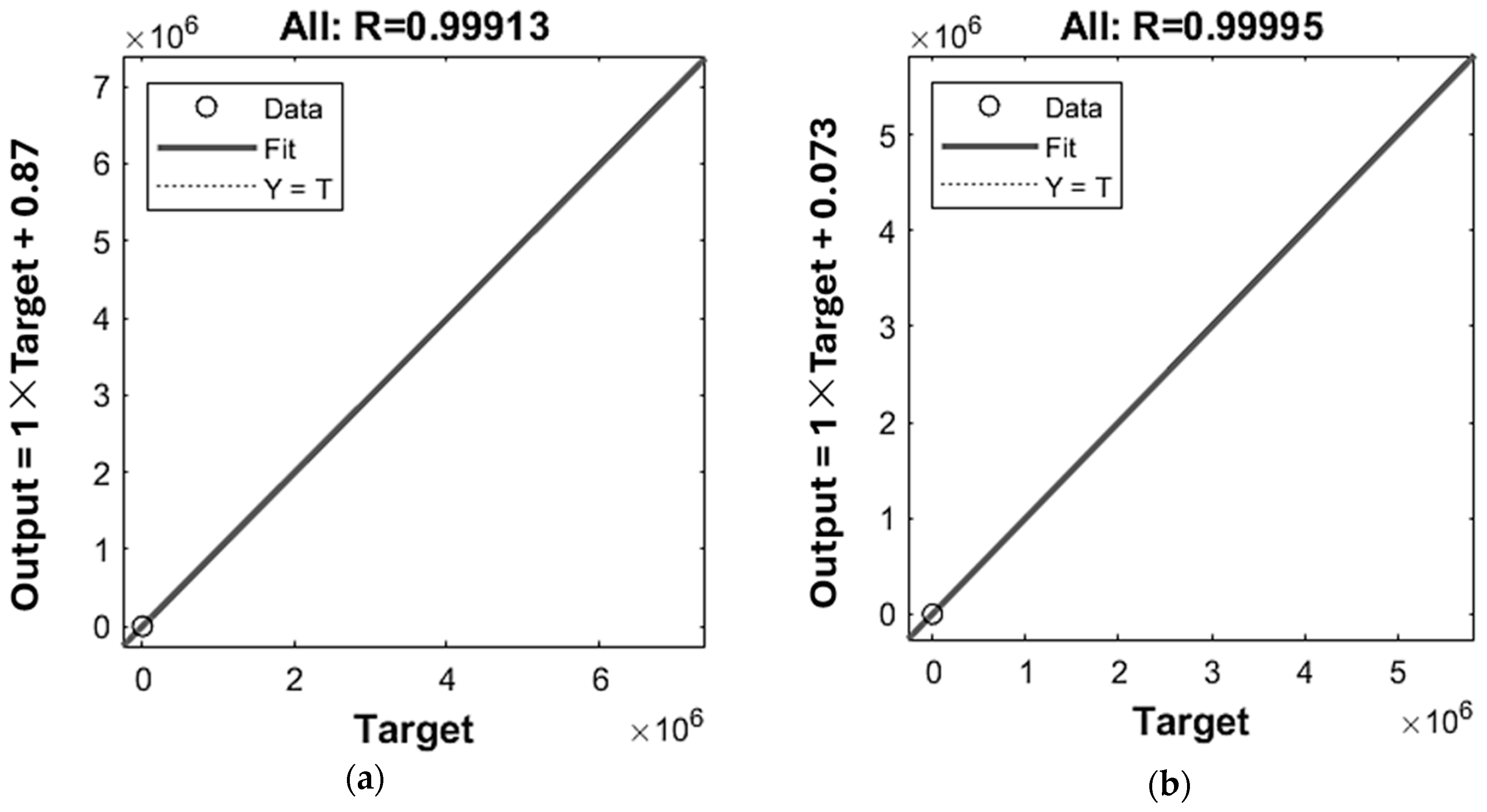
Model	Inputs	Outputs	ANN Layout	Checks
				R				MSE	MAPE (%)
				Training	Testing	Validation	Whole Dataset
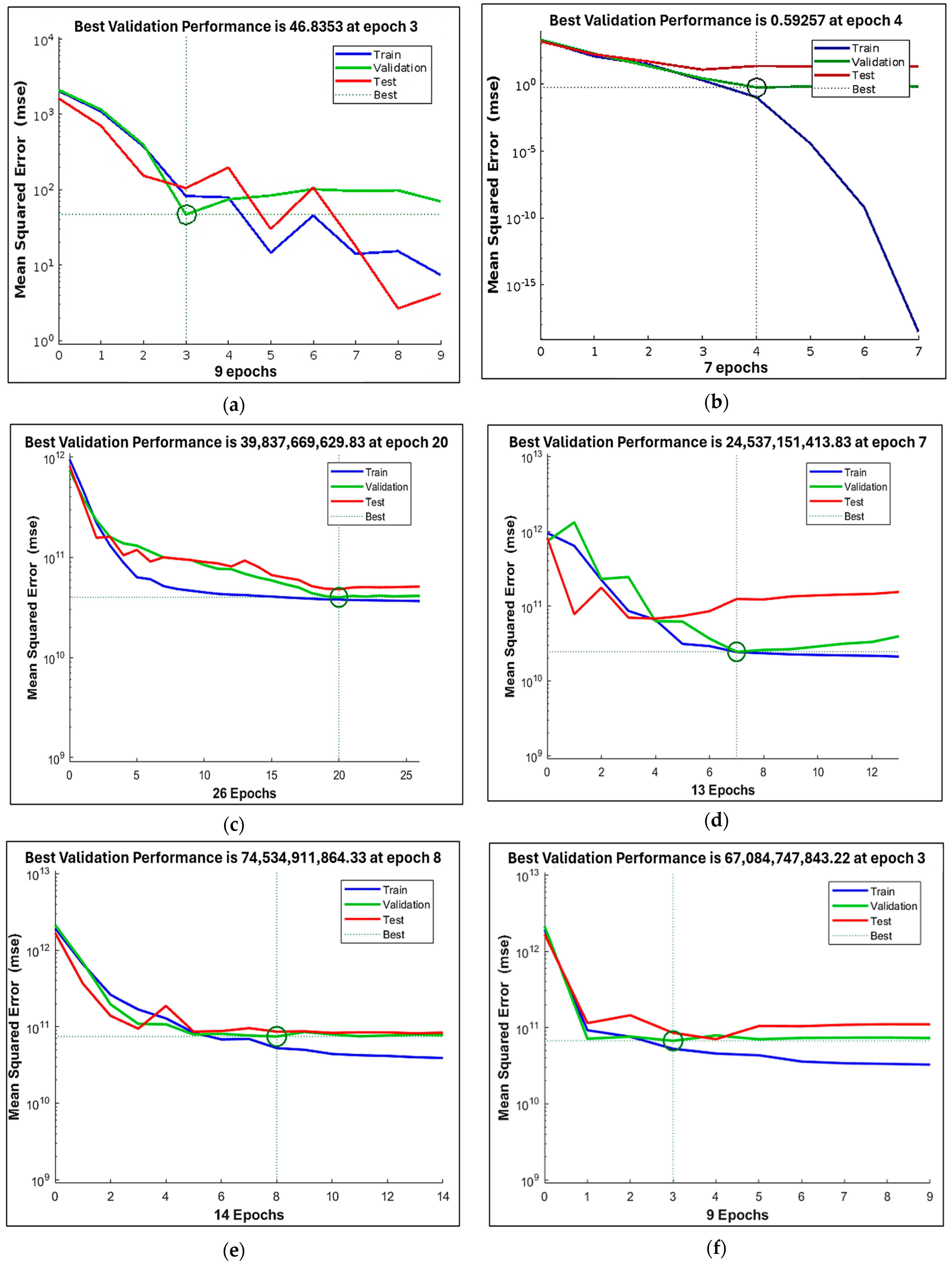
1	Monthly average: air temperature (°C) total daily global solar radiation (kWh/m2) total daily solar intensity (cal/cm2) evaporation (mm) evapotranspiration (mm)	Monthly average: volume (hm3) incoming water flow rate (m3/day) outgoing water flow rate (m3/day) water level (m)	5-10-4	RProp: 0.9908 LM: 1	RProp: 1 LM: 1	RProp: 1 LM: 1	RProp: 0.99913 LM: 0.99995	RProp: 46.8353 LM: 0.59257	RProp: 13.5 LM: 1.31
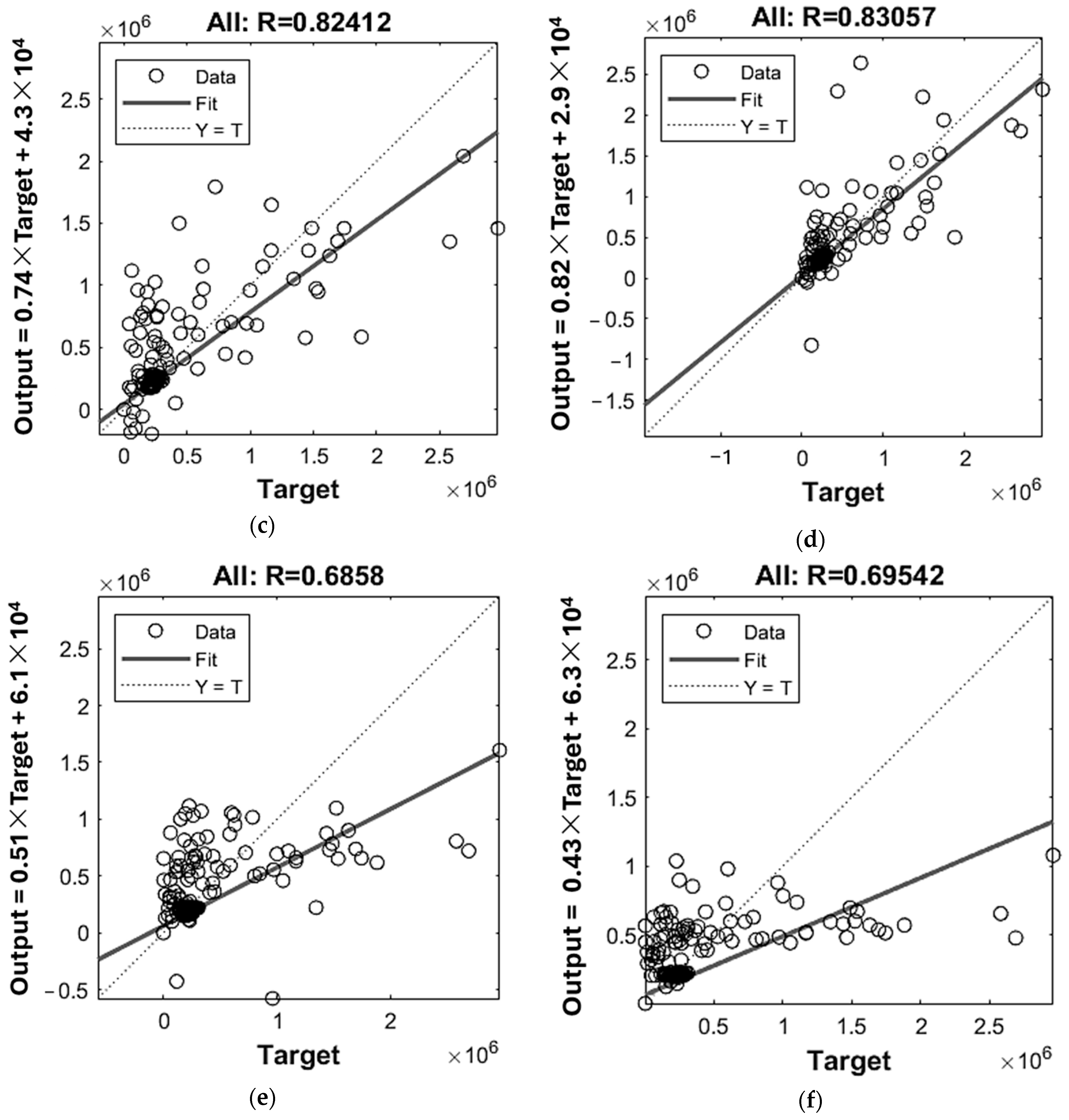
2	Monthly average: wind speed (m/s) vapor pressure (hPa)	Monthly average: volume (hm3) incoming water flow rate (m3/day) outgoing water flow rate (m3/day) water level (m)	2-10-4	RProp: 0.83633 LM: 0.89876	RProp: 0.79397 LM: 0.62345	RProp: 0.85413 LM: 0.93957	RProp: 0.82412 LM: 0.83057	RProp: 4.0 × 1010 LM: 2.4 × 1010	RProp: 38.88 LM: 37.3
3	Monthly average: precipitation (mm) total snow depth (cm) relative humidity (%)	Monthly average: volume (hm3) incoming water flow rate (m3/day) outgoing water flow rate (m3/day) water level (m)	3-10-4	RProp: 0.69929 LM: 0.69352	RProp: 0.70283 LM: 0.7626	RProp: 0.60448 LM: 0.65079	RProp: 0.6858 LM: 0.69542	RProp: 7.4 × 1010 LM: 6.7 × 1010	RProp: 152.52 LM: 184.27

. This can be portrayed by having an insight into the R, MSE, and MAPE values for all the models that model 1 gave the best fit. Considering both algorithms, Model 1 had a high R-value (0.99) for the entire dataset. In addition, it had the lowest MSE (0.59 in the case of LM and 46.8 using RProp) compared to the other models, which had considerably larger errors in the validation stage. In other words, all the models had the same output parameters, but the analysis showed that the model using air temperature, global solar radiation, solar intensity, evaporation, and evapotranspiration as input meteorological parameters defined and correlated best with the change in the hydrological data of the Doğancı dam. Hence, it can be interpreted that a change in the meteorological parameters of Model 1 can significantly impact the dam’s water volume, flow rates, and level. In previous studies, it has been observed that temperature and evaporation parameters (used in Model 1) had a greater effect on precipitation-flow changes and hydrological droughts in water resources [64,65].

The magnitude of errors in Models 2 and 3 was quite high (ranging between 2.4 × 10¹⁰ to 7.4 × 10¹⁰ overall), and R-values were also lower in comparison to Model 1 (approximately 0.82 to 0.83 in the case of Model 2 and 0.68 to 0.70 for Model 3). The inputs for Model 2 were wind speed and vapor pressure. Likewise, precipitation, snow depth, and relative humidity were the inputs for Model 3.

Model 2 indicated a good correlation between the observed and predicted values. However, considering the error, which was reasonably high (regardless of the type of training algorithm used), it may not be the preferred model for future prediction of the hydrology of the Doğancı dam. Model 3 showed a similar trend, with a lower correlation (up to 0.70) than Model 2 for the observed and predicted values of the hydrological parameters of the dam.

The mean absolute percentage error presented in Table 2 also offers a clear comparison of the predictive accuracy of Model 1. The aforementioned model trained using the Levenberg-Marquardt algorithm yielded the lowest MAPE value of 1.31%, indicating excellent predictive and generalization capabilities. In contrast, the same model trained with the resilient backpropagation algorithm yielded a higher MAPE of 13.5%, although it was still within an acceptable range. Model 2 showed moderate performance, with MAPE values ranging between 37% and 38%. Model 3 had the highest MAPE, reaching 184.27%, which indicated a substantial deviation between the predicted and observed output values. MAPE values over 100% exhibited nonlinear and weak correlations between the input and output parameters, leading to reduced predictive power. These limitations reduce the model’s ability to generalize effectively and highlight the importance of input selection. Therefore, this discussion further strengthens the reliability of Model 1, making it the optimal choice for forecasting the hydrological parameters of the Doğancı dam.

The acquired mean squared error and coefficient values from Model 1 were compared with those obtained from previous studies (

Table 3. References to past studies that used meteorological parameters as inputs to predict the water quantity parameters of a dam.

Study No.	Dam (Location)	Inputs (Meteorological Parameters)	Outputs (Hydrological Parameters)	Errors	Correlation Coefficient	Reference
1	Yalova Gökçe (Turkey)	Annual precipitation	Dam’s water level	0.11	0.87	[53]
2	Norris (America)	Annual precipitation and air temperature	Inflow volume to the dam and water level	11	0.81	[24]
3	Doroozdan (Iran)	Monthly precipitation	Inflow volume to the dam	34.60 × 106	0.64	[62]
4	Asa and Kampe (Nigeria)	Annual air temperature, precipitation, and evapotranspiration	Inflow rate to the dam	-	0.99	[25]
5	Batu (Malaysia)	Daily air temperature, wind speed, relative humidity, precipitation, sunshine duration, and solar radiation	Evaporation from the dam	1.22	0.96	[23]
6	Yarseli (Turkey)	Daily precipitation	Dam’s water level	0.135	0.99	[54]

). When considering the errors, the MSE obtained using the LM training algorithm in Model 1 was 0.59, which was higher than that of Studies 1 and 6, as listed in Table 3. However, it was still lower than similar studies on the Norris, Doroozdan, Asa, Kampe, and Batu dams, which still show its acceptability for predictions. The error for Model 1 using the Rprop training algorithm was 46.84, higher than all the enlisted studies except Study 3 (Doroozdan dam). Because the errors must be as low as possible, it was suggested that the LM training algorithm performed better in our study.

However, when comparing the correlation coefficients, R in Model 1 was approximated to be 0.99 for the entire dataset. This R-value was closest to those of studies 4, 5, and 6 and higher than those of the other relevant studies listed in Table 3. When discussing the training algorithms, LM and Rprop showed almost the same high correlation between the observed and predicted outcomes.

In addition to other inputs, precipitation is the preferred meteorological parameter when simulating water availability in dams (as perceived from previous studies). However, in our study, Model 1, which performed better than the other tested models, did not include precipitation as an input. Therefore, this study reveals that precipitation is not the sole parameter for such determinations. Rather, other parameters, such as air temperature, solar intensity or radiation, evaporation, or evapotranspiration, can also provide valuable outcomes regarding the water volume, flow rate, and/or level of the dam. The closest example of such a case is a study by Benzaghta, et al. [23] on the Batu dam.

Other modeling approaches have also been applied for dam inflow prediction, yielding varying levels of performance. For instance, Awan and Bae [66] utilized an adaptive neuro-fuzzy inference system to forecast long-term monthly inflows to major dams in South Korea using diverse meteorological input variables. Their optimal model achieved a correlation coefficient of 0.97. In a separate study on Egypt’s Aswan Dam, a forecast-based adaptive reservoir operation framework was implemented to evaluate the dam’s long-term resilience to climate change scenarios. This approach, which employed monthly precipitation and temperature data, achieved a maximum correlation coefficient of 0.92 [67]. Another model, the variation analog model, was modified by Amnatsan et al. [68] for the standardized inflow management of the Sirikit dam in Thailand during low-flow and high-flow periods. Their model produced a minimum root mean square error of 115.55 and a peak R-value of 0.98. In comparison, the present research demonstrates competitive predictive performance, further validating the reliability and robustness of the proposed ANN-based model.

The regression plots are shown in Figure 5. The line labeled Y = T represents the ideal case, where the predicted output exactly matches the actual output value. Hence, there was perfect agreement between the model prediction and actual data. The closer the regression fit line to Y = T, the better the predictions. In Model 1, the regression line lay almost exactly on the Y = T line, demonstrating that it fitted the target (water volume, flow rates, and water level of the dam) very well. In contrast, the plots for Models 2 and 3 exhibited significant deviations from the Y = T line, indicating underfitting and poor predictive alignment. The data are dispersed and have many outliers in Cleavage models 2 and 3, which shows that the data are heteroscedastic. This term indicates a significant variance in the errors for Models 2 and 3, which causes the data points on the regression graphs to move away from the Y = T line. This again revealed that Models 2 and 3 may not provide accurate predictions as Model 1.

The second objective was to identify the best training algorithm among the resilient backpropagation and Levenberg-Marquardt algorithms. Figure 6 shows the graphs of the MSE trend for the training, validation, and test sets across epochs. In all cases, the LM-trained models exhibited lower errors than those trained with Rprop. It can also be noted that the LM algorithm yielded the best performance for the models in terms of convergence with a lower number of epochs. Hence, stabilizing earlier indicates faster learning and better generalization. Model 1, which outperformed the other models, demonstrated high fluctuations in the error curves. Therefore, it indicates higher validation losses and lower predictive accuracy. Overall, the LM algorithm outperformed Rprop in all three models in terms of convergence speed, error minimization, and predictive reliability.

In addition, the gradient graphs in the training state showed similar outcomes (Figure 7). The gradient is a vector of partial derivatives that indicates the extent to which the error changes with respect to the weight in the networks and adjusts the weights to minimize the error. If the gradient is large, the model is far from the optimum, and vice versa. The Rprop algorithm displayed a slower and less smooth gradient reduction. Hence, this indicates that the Rprop training algorithm struggled to efficiently minimize the loss function for complex input patterns or non-linear relationships. This may contribute to suboptimal prediction accuracy and higher error metrics (as seen in the MAPE and MSE values). The LM algorithm reflected comparatively lower gradient values across all models, further confirming its suitability for training artificial neural networks in hydrological applications.

Resilient backpropagation has also been documented in the previous literature to have slow training speeds and instability over time, which can lead to oscillatory behavior during learning and susceptibility to getting stuck in local minima. In contrast, convergence is faster with the Levenberg–Marquardt algorithm, which offers a more efficient and stable approach for training artificial neural networks [69,70].

Analysis of variance (ANOVA) was performed on JASP (version 0.16.3) [71] for the correlation, mean squared error, and mean absolute percentage error values obtained from the neural network using the two training algorithms for all the tested models. As shown in

Table 4. ANOVA results for (a) R, (b) MSE, and (c) MAPE values of the models when comparing algorithms.

Cases	Sum of Squares	df	Mean Square	F	p	η2
Algorithms	5.298 × 10−5	1	5.298 × 10−5	0.002	0.965	5.541 × 10−4
Residuals	0.096	4	0.024
(a)
Algorithms	8.627 × 1019	1	8.627 × 1019	0.068	0.807	0.017
Residuals	5.086 × 1021	4	1.272 × 1021
(b)
Algorithms	54.361	1	54.361	0.007	0.936	0.002
Residuals	29,756.237	4	7439.059
(c)

(a), for a comparison between the R values for the examined algorithms, the p-value is 0.965 (as p > 0.05 with a 95% confidence level), which indicates that the difference was not significant between the R values provided for different models. The effect size (η²) was also minimal (5.541 × 10⁻⁴), indicating that the difference between the two training algorithms was negligible. The same was true for the MSE and MAPE values for both algorithms, where the p-values were 0.807 and 0.936, and the effect sizes were 0.017 and 0.002, respectively. Hence, both training algorithms performed the same with our data and can be applied when using feedforward neural networks to determine the climatic effects on the hydrology of a dam, as statistically proven.

However, visually interpreting the results and based on the discussion on the performance and training state of the models, a slight edge can be given to the Levenberg-Marquardt algorithm, where correlation values for all the studied models were slightly higher and error values lower compared to the resilient backpropagation training algorithm in most of the cases. The mean squared error values of Model 1 with the Levenberg-Marquardt training algorithm were also well related to previous studies in similar fields.

4. Conclusions

Climate change has adversely affected the environment. However, its impact on water resources is alarming, especially on the water budget of water bodies. This study investigated one such impact. Artificial neural networks were used to develop and predict the influence of meteorological changes on the hydrological characteristics of the Doğancı dam, which included volume, inflows, outflows, and the water level of the Doğancı dam. The results concluded that Model 1 performed the best, i.e., air temperature, solar radiation, solar intensity, evaporation, and evapotranspiration best predicted the water volume, flow rates, and water level of the Doğancı dam. Model 1 had the least mean squared and mean absolute percentage error, i.e., 0.59 and 1.31%, respectively, and the highest R (0.99) for the whole dataset among the other defined models tested using the Levenberg-Marquardt training algorithm. The analysis was based on the correlation values and mean squared errors. In addition, it was observed that using resilient backpropagation or Levenberg-Marquardt training algorithms does not statistically affect the analytical results. However, visually comparing the R, MSE, and MAPE values, graphical interpretations, and convergence patterns, the Levenberg-Marquardt algorithm performs slightly better than the resilient backpropagation. Hence, this study describes the appropriateness and efficiency of artificial neural networks for predictions in hydrology and the meteorological parameters that can most precisely simulate the water availability of dams. The results of this study offer practical value for government bodies, water resource planners, and climate adaptation policymakers. Accurate prediction of dam hydrology under changing climates can inform proactive reservoir management, drought preparedness, and long-term infrastructure planning.

However, certain limitations of this study must be acknowledged. The models were trained and tested on data from previous years without incorporating future climate projections, which may constrain their applicability for long-term planning. Additionally, the model’s performance is contingent on the quality and completeness of the input data, which may compromise prediction reliability. Future research should focus on integrating downscaled climate model outputs based on future scenarios and testing their generalizability across different hydrological systems. Additionally, future studies may explore other established algorithms, such as evolutionary algorithms, for training and comparing ANN models.

References

- Cooper, S.D.; Lake, P.S.; Sabater, S.; Melack, J.M.; Sabo, J.L. The effects of land use changes on streams and rivers in mediterranean climates. Hydrobiologia 2013, 719, 383–425. [Google Scholar] [CrossRef]
- Kondolf, G.M.; Gao, Y.; Annandale, G.W.; Morris, G.L.; Jiang, E.; Zhang, J.; Cao, Y.; Carling, P.; Fu, K.; Guo, Q.; et al. Sustainable sediment management in reservoirs and regulated rivers: Experiences from five continents. Earth’s Future 2014, 2, 256–280. [Google Scholar] [CrossRef]
- Hogeboom, R.J.; Knook, L.; Hoekstra, A.Y. The blue water footprint of the world’s artificial reservoirs for hydroelectricity, irrigation, residential and industrial water supply, flood protection, fishing and recreation. Adv. Water Resour. 2018, 113, 285–294. [Google Scholar] [CrossRef]
- Chamoglou, M.; Papadimitriou, T.; Kagalou, I. Key-descriptors for the functioning of a Mediterranean reservoir: The case of the new Lake Karla-Greece. Environ. Process. 2014, 1, 127–135. [Google Scholar] [CrossRef]
- Mahmood, R.; Pielke Sr, R.A.; Hubbard, K.G.; Niyogi, D.; Dirmeyer, P.A.; McAlpine, C.; Carleton, A.M.; Hale, R.; Gameda, S.; Beltrán-Przekurat, A.; et al. Land cover changes and their biogeophysical effects on climate. Int. J. Climatol. 2014, 34, 929–953. [Google Scholar] [CrossRef]
- Casserly, C.M.; Turner, J.N.; O’sullivan, J.J.; Bruen, M.; Bullock, C.; Atkinson, S.; Kelly-Quinn, M. Impact of low-head dams on bedload transport rates in coarse-bedded streams. Sci. Total Environ. 2020, 716, 136908. [Google Scholar] [CrossRef]
- Zhang, J.; Zhu, Y.; Zhang, X.; Ye, M.; Yang, J. Developing a Long Short-Term Memory (LSTM) based model for predicting water table depth in agricultural areas. J. Hydrol. 2018, 561, 918–929. [Google Scholar] [CrossRef]
- Awad, M.; Zaid-Alkelani, M. Prediction of water demand using artificial neural networks models and statistical model. Int. J. Intell. Syst. Appl. 2019, 11, 40. [Google Scholar] [CrossRef]
- Elshorbagy, A.; Simonovic, S.; Panu, U. Performance evaluation of artificial neural networks for runoff prediction. J. Hydrol. Eng. 2000, 5, 424–427. [Google Scholar] [CrossRef]
- McJannet, D.; Cook, F.; Burn, S. Comparison of techniques for estimating evaporation from an irrigation water storage. Water Resour. Res. 2013, 49, 1415–1428. [Google Scholar] [CrossRef]
- Ouali, D.; Chebana, F.; Ouarda, T.B. Fully nonlinear statistical and machine-learning approaches for hydrological frequency estimation at ungauged sites. J. Adv. Model. Earth Syst. 2017, 9, 1292–1306. [Google Scholar] [CrossRef]
- Yaseen, Z.M. A new benchmark on machine learning methodologies for hydrological processes modelling: A comprehensive review for limitations and future research directions. Knowl.-Based Eng. Sci. 2023, 4, 65–103. [Google Scholar] [CrossRef]
- Nourani, V.; Molajou, A.; Najafi, H.; Danandeh Mehr, A. Emotional ANN (EANN): A new generation of neural networks for hydrological modeling in IoT. In Artificial Intelligence in IoT; Springer: Cham, Switzerland; Geneva, Switzerland, 2019; pp. 45–61. [Google Scholar]
- Tabbussum, R.; Dar, A.Q. Performance evaluation of artificial intelligence paradigms—Artificial neural networks, fuzzy logic, and adaptive neuro-fuzzy inference system for flood prediction. Environ. Sci. Pollut. Res. 2021, 28, 25265–25282. [Google Scholar] [CrossRef]
- Yaseen, Z.M.; Naganna, S.R.; Sa’adi, Z.; Samui, P.; Ghorbani, M.A.; Salih, S.Q.; Shahid, S. Hourly river flow forecasting: Application of emotional neural network versus multiple machine learning paradigms. Water Resour. Manag. 2020, 34, 1075–1091. [Google Scholar] [CrossRef]
- Oyebode, O.; Stretch, D. Neural network modeling of hydrological systems: A review of implementation techniques. Nat. Resour. Model. 2019, 32, e12189. [Google Scholar] [CrossRef]
- Huang, Y. Advances in artificial neural networks–methodological development and application. Algorithms 2009, 2, 973–1007. [Google Scholar] [CrossRef]
- Üneş, F.; Demirci, M.; Kişi, Ö. Prediction of millers ferry dam reservoir level in USA using artificial neural network. Period. Polytech. Civ. Eng. 2015, 59, 309–318. [Google Scholar] [CrossRef]
- Valipour, M.; Banihabib, M.E.; Behbahani, S.M.R. Comparison of the ARMA, ARIMA, and the autoregressive artificial neural network models in forecasting the monthly inflow of Dez dam reservoir. J. Hydrol. 2013, 476, 433–441. [Google Scholar] [CrossRef]
- Hadiyan, P.P.; Moeini, R.; Ehsanzadeh, E. Application of static and dynamic artificial neural networks for forecasting inflow discharges, case study: Sefidroud Dam reservoir. Sustain. Comput. Inform. Syst. 2020, 27, 100401. [Google Scholar] [CrossRef]
- Rani, S.; Parekh, F. Application of artificial neural network (ANN) for reservoir water level forecasting. Int. J. Sci. Res. 2014, 3, 1077–1082. [Google Scholar]
- Üneş, F.; Demirci, M.; Başar, B.; Kaya, Y.Z.; Varçın, H. Estimating dam reservoir level fluctuations using data-driven techniques. Pol. J. Environ. Stud. 2019, 28, 3451–3462. [Google Scholar] [CrossRef] [PubMed]
- Benzaghta, M.A.; Mohammed, T.A.; Ghazali, A.H.; Soom, M.A.M. Prediction of evaporation in tropical climate using artificial neural network and climate based models. Sci. Res. Essays 2012, 7, 3133–3148. [Google Scholar]
- Rungee, J.; Kim, U. Long-term assessment of climate change impacts on Tennessee Valley Authority reservoir operations: Norris Dam. Water 2017, 9, 649. [Google Scholar] [CrossRef]
- Salami, A.W.; Ibrahim, H.; Sojobi, A.O. Evaluation of impact of climate variability on water resources and yield capacity of selected reservoirs in the north central Nigeria. Environ. Eng. Res. 2015, 20, 290–297. [Google Scholar] [CrossRef]
- Ley, A.; Bormann, H.; Casper, M. Climate change impact assessment on a German lowland river using long short-term memory and conceptual hydrological models. J. Hydrol. Reg. Stud. 2025, 59, 102426. [Google Scholar] [CrossRef]
- Katip, A.; Anwar, A. Modeling the Influence of Climate Change on the Water Quality of Doğancı Dam in Bursa, Turkey, Using Artificial Neural Networks. Water 2025, 17, 728. [Google Scholar] [CrossRef]
- Kim, T.; Shin, J.-Y.; Kim, H.; Kim, S.; Heo, J.-H. The use of large-scale climate indices in monthly reservoir inflow forecasting and its application on time series and artificial intelligence models. Water 2019, 11, 374. [Google Scholar] [CrossRef]
- Lee, J. A Study on the Improvement of Flood Season in Korea Considering the 21st Century Observations. Master’s Thesis, Department of Civil and Environmental Engineering, College of Engineering, Seoul National University, Seoul, Republic of Korea, 2022. Available online: https://dcollection.snu.ac.kr/common/orgView/000000173218 (accessed on 26 February 2025).
- IPCC. Climate Change 2022: Mitigation of Climate Change; Cambridge University Press: Cambridge, UK, 2022. [Google Scholar]
- Wang, L.; Li, Y.; Biswas, A.; Zhao, Y.; Niu, B.; Siddique, K.H. Assessing climate change and human impacts on runoff and hydrological droughts in the Yellow River Basin using a machine learning-enhanced hydrological modeling approach. J. Environ. Manag. 2025, 380, 125091. [Google Scholar] [CrossRef]
- Chen, D.; Hu, W.; Li, Y.; Zhang, C.; Lu, X.; Cheng, H. Exploring the temporal and spatial effects of city size on regional economic integration: Evidence from the Yangtze River Economic Belt in China. Land Use Policy 2023, 132, 106770. [Google Scholar] [CrossRef]
- Xu, L.; Pombo, N.; Pires, I.M.; Garcia, N.M. Is Overfitting in a Neural Network a Reliable Model for the Recognition of Activities of Daily Living? In Proceedings of the 5th EAI International Conference on Smart Objects and Technologies for Social Good, Valencia, Spain, 25–27 September 2019; pp. 223–226. [Google Scholar]
- Pachauri, R.K.; Pachauri, R.K.; Allen, M.R.; Barros, V.R.; Broome, J.; Cramer, W.; Christ, R.; Church, J.A.; Clarke, L.; Dahe, Q.; et al. Contribution of Working Groups I, II and III to the Fifth Assessment Report of the Intergovernmental Panel on Climate Change in Climate Change 2014: Synthesis Report; IPCC: Geneva, Switzerland, 2014. [Google Scholar]
- BUSKI. Baraj Doluluk Oranları. Available online: https://www.buski.gov.tr/baraj-detay (accessed on 7 January 2025).
- Koç, A.A.; Codron, J.M.; Tekelioğlu, Y.; Lemeilleur, S.; Tozanli, S.; Aksoy, Ş.; Bignebat, C.; Demirer, R.; Mencet, N. Restructuring of Agrifood Chains in Turkey. In Regoverning Markets Agrifood Sector Studies (A); IIED: London, UK, 2007. [Google Scholar]
- Apaydin, H.; Feizi, H.; Sattari, M.T.; Colak, M.S.; Shamshirband, S.; Chau, K.-W. Comparative analysis of recurrent neural network architectures for reservoir inflow forecasting. Water 2020, 12, 1500. [Google Scholar] [CrossRef]
- Okkan, U. Aylık Yağış ve Sıcaklık Değişimlerinin İzmir Içme Suyu Havzalarının Akımlarına Etkileri. Master’s Thesis, Fen Bilimleri Enstitüsü, Dokuz Eylül Üniversitesi, İzmir, Turkey, 2009. [Google Scholar]
- Raşit, A. Namazgâh Barajında Meteorolojik Veriler Kullanılarak Yapay Sinir Ağları ile Akışın Tahmin Edilmesi. Master’s Thesis, Fen Bilimleri Enstitüsü, Kocaeli Üniversitesi, İzmit, Turkey, 2019. Available online: http://dspace.kocaeli.edu.tr:8080/xmlui/handle/11493/16790 (accessed on 12 December 2024).
- Mata, J. Interpretation of concrete dam behaviour with artificial neural network and multiple linear regression models. Eng. Struct. 2011, 33, 903–910. [Google Scholar] [CrossRef]
- Ozsoy, G.; Aksoy, E.; Karaata, E. Estimating soil loss of Doganci Dam watershed, northwest Turkey and lifetime analyze of Doganci Dam using multi-year remotely sensed data and GIS techniques. Soil-Water J. 2013, 2, 927–934. [Google Scholar]
- Stotz, C.L. The Bursa region of Turkey. Geogr. Rev. 1939, 29, 81–100. [Google Scholar] [CrossRef]
- Erünal, E. Examining age structure and estimating mortality rates in Ottoman Bursa using mid-nineteenth-century population registers. Middle East. Stud. 2020, 57, 179–196. [Google Scholar] [CrossRef]
- Noor, R.M.; Ahmad, Z.; Don, M.M.; Uzir, M. Modelling and control of different types of polymerization processes using neural networks technique: A review. Can. J. Chem. Eng. 2010, 88, 1065–1084. [Google Scholar] [CrossRef]
- Tabari, H.; Talaee, P.H. Reconstruction of river water quality missing data using artificial neural networks. Water Qual. Res. J. Can. 2015, 50, 326–335. [Google Scholar] [CrossRef]
- O’Reilly, G.; Bezuidenhout, C.; Bezuidenhout, J. Artificial neural networks: Applications in the drinking water sector. Water Supply 2018, 18, 1869–1887. [Google Scholar] [CrossRef]
- Najah, A.; El-Shafie, A.; Karim, O.A.; El-Shafie, A.H. Application of artificial neural networks for water quality prediction. Neural Comput. Appl. 2013, 22, 187–201. [Google Scholar] [CrossRef]
- Kang, B.; Kim, Y.D.; Lee, J.M.; Kim, S.J. Hydro-environmental runoff projection under GCM scenario downscaled by artificial neural network in the Namgang Dam watershed, Korea. KSCE J. Civ. Eng. 2015, 19, 434–445. [Google Scholar] [CrossRef]
- Kruczyk, M. Long series of GNSS integrated precipitable water as a climate change indicator. Rep. Geod. Geoinform. 2015, 99, 1–18. [Google Scholar] [CrossRef]
- El-Mahdy, M.E.-S.; El-Abd, W.A.; Morsi, F.I. Forecasting lake evaporation under a changing climate with an integrated artificial neural network model: A case study Lake Nasser, Egypt. J. Afr. Earth Sci. 2021, 179, 104191. [Google Scholar] [CrossRef]
- Svozil, D.; Kvasnicka, V.; Pospichal, J. Introduction to multi-layer feed-forward neural networks. Chemom. Intell. Lab. Syst. 1997, 39, 43–62. [Google Scholar] [CrossRef]
- Mohamad, R.N.M.R.; Ishak, W.H.W. Forecasting the flood stage of a reservoir based on the changes in upstream rainfall pattern. J. Technol. Oper. Manag. 2019, 14, 46–52. [Google Scholar]
- Damla, Y.; Temiz, T.; Keskin, E. Yapay sinir ağı kullanılarak su seviyesinin tahmin edilmesi: Yalova Gökçe barajı örneği. Kırklareli Üniversitesi Mühendislik Fen Bilim. Derg. 2020, 6, 32–49. [Google Scholar] [CrossRef]
- Çalım, M.M. Estimation of Dam Reservoir Level with Artificial Neural Network Method. Master’s Thesis, Mustafa Kemal Üniversitesi, Antakya, Turkey, 2008. Available online: https://tez.yok.gov.tr/UlusalTezMerkezi/tezDetay.jsp?id=tPtS_heSMyicaKWhD0vd6w&no=hXyjBcHCUojyy4SSrKgk7A (accessed on 16 January 2025).
- Igel, C.; Toussaint, M.; Weishui, W. Rprop using the natural gradient. Trends Appl. Constr. Approx. 2005, 151, 259–272. [Google Scholar] [CrossRef]
- Gavin, H.P. The Levenberg-Marquardt Algorithm for Nonlinear Least Squares Curve-Fitting Problems. Master’s Thesis, Department of Civil and Environmental Engineering, Duke University, Durham, CA, USA, 2019. [Google Scholar]
- Taylor, R. Interpretation of the correlation coefficient: A basic review. J. Diagn. Med. Sonogr. 1990, 6, 35–39. [Google Scholar] [CrossRef]
- Wu, S.; McAuley, K.; Harris, T. Selection of simplified models: I. Analysis of model-selection criteria using mean-squared error. Can. J. Chem. Eng. 2011, 89, 148–158. [Google Scholar] [CrossRef]
- Chicco, D.; Warrens, M.J.; Jurman, G. The coefficient of determination R-squared is more informative than SMAPE, MAE, MAPE, MSE and RMSE in regression analysis evaluation. Peerj Comput. Sci. 2021, 7, e623. [Google Scholar] [CrossRef]
- Mathworks. Deep Learning Toolbox-Design, Train, Analyze, and Simulate Deep Learning Networks. In Deep Learning Toolbox; The Mathworks, Inc.: Natick, MA, USA, 2022. [Google Scholar]
- Wahir, N.; Nor, M.; Rusiman, M.; Gopal, K. Treatment of outliers via interpolation method with neural network forecast performances. J. Phys. Conf. Ser. 2017, 995, 012025. [Google Scholar] [CrossRef]
- Rezaeianzadeh, M.; Stein, A.; Cox, J.P. Drought forecasting using Markov chain model and artificial neural networks. Water Resour. Manag. 2016, 30, 2245–2259. [Google Scholar] [CrossRef]
- Üneş, F.; Varçın, H.; Dindar, K.K. Yapay sinir ağları yaklaşımı ile tahtaköprü barajındaki aylık buharlaşma tahmini. Eng. Sci. 2011, 6, 114–125. [Google Scholar]
- Khosravi, K.; Farooque, A.A.; Karbasi, M.; Ali, M.; Heddam, S.; Faghfouri, A.; Abolfathi, S. Enhanced water quality prediction model using advanced Hybridized resampling alternating tree-based and deep learning algorithms. Environ. Sci. Pollut. Res. 2025, 32, 6405–6424. [Google Scholar] [CrossRef] [PubMed]
- Khosravi, K.; Farooque, A.A.; Naghibi, A.; Heddam, S.; Sharafati, A.; Hatamiafkoueieh, J.; Abolfathi, S. Enhancing pan evaporation predictions: Accuracy and uncertainty in hybrid machine learning models. Ecol. Inform. 2025, 85, 102933. [Google Scholar] [CrossRef]
- Awan, J.A.; Bae, D.-H. Improving ANFIS based model for long-term dam inflow prediction by incorporating monthly rainfall forecasts. Water Resour. Manag. 2014, 28, 1185–1199. [Google Scholar] [CrossRef]
- Eldardiry, H.; Hossain, F. The value of long-term streamflow forecasts in adaptive reservoir operation: The case of the High Aswan Dam in the transboundary Nile River basin. J. Hydrometeorol. 2021, 22, 1099–1115. [Google Scholar] [CrossRef]
- Amnatsan, S.; Yoshikawa, S.; Kanae, S. Improved forecasting of extreme monthly reservoir inflow using an analogue-based forecasting method: A case study of the Sirikit Dam in Thailand. Water 2018, 10, 1614. [Google Scholar] [CrossRef]
- Beale, M.H.; Hagan, M.T.; Demuth, H.B. Neural network toolbox. In User’s Guide, MathWorks; The Mathworks, Inc.: Natick, MA, USA, 2010; Volume 2, pp. 77–81. [Google Scholar]
- Adeloye, A.; De Munari, A. Artificial neural network based generalized storage–yield–reliability models using the Levenberg–Marquardt algorithm. J. Hydrol. 2006, 326, 215–230. [Google Scholar] [CrossRef]
- Goss-Sampson, M. Statistical analysis in JASP: A Guide for Students; JASP: Amsterdam, The Netherlands, 2019. [Google Scholar]