Lightweight YOLOv8-Based Model for Weed Detection in Dryland Spring Wheat Fields

Abstract

Efficient weed detection in dryland spring wheat fields is crucial for sustainable agriculture, as it enables targeted interventions that reduce herbicide use, minimize environmental impact, and optimize resource allocation in water-limited farming systems. This paper presents HSG-Net, a novel lightweight object detection model based on YOLOv8 for weed identification in dryland spring wheat fields. The proposed architecture integrates three key innovations: an HGNetv2 backbone for efficient feature extraction, C2f-S modules with star-shaped attention mechanisms for enhanced feature representation, and Group Head detection heads for parameter-efficient prediction. Experiments on a dataset of eight common weed species in dryland spring wheat fields show that HSG-Net improves detection accuracy while cutting computational costs, outperforming modern deep learning approaches. The model effectively addresses the unique challenges of weed detection in dryland agriculture, including visual similarity between crops and weeds, variable illumination conditions, and complex backgrounds. Ablation studies confirm the complementary contributions of each architectural component, with the full HSG-Net model achieving an optimal balance between accuracy and resource efficiency. The lightweight nature of HSG-Net makes it particularly suitable for deployment on resource-constrained devices used in precision agriculture, enabling real-time weed detection and targeted intervention in field conditions. This work represents an important advancement in developing practical deep learning solutions for sustainable weed management in dryland farming systems.

1. Introduction

Weed infestation represents one of the most significant threats to global agricultural productivity, responsible for estimated annual crop yield losses of 34% worldwide [1]. Dryland spring wheat production systems, characterized by limited and often erratic precipitation (≤600 mm annually), represent a significant portion of global wheat acreage and are critical for food security in many semi-arid regions [2]. Spring wheat, planted in early spring rather than fall, faces unique weed management challenges as its growing cycle coincides with the emergence of problematic weed species like wild oat (Avena fatua), creating competition for limited soil moisture and nutrients during critical early growth stages [3].

According to Fahad et al. [4], these systems are particularly vulnerable to weed interference due to the already constrained water and nutrient resources. In such conditions, weeds represent a major bottleneck to productivity, with weed infestation accounting for more than 48% loss of potential wheat yield in some regions. The magnitude of yield losses depends on weed species, density, emergence timing, and crop management practices. Reductions are most severe when limited resources must be shared and weeds emerge simultaneously with the crop.

Traditional weed management relies heavily on broadcast herbicide applications, contributing to environmental pollution, herbicide resistance development, and escalating production costs [5]. The concept of precision agriculture, particularly site-specific weed management, has emerged as a promising approach to address these challenges by enabling targeted interventions only where weeds are present [6].

The successful implementation of site-specific weed management systems fundamentally depends on accurate and efficient weed detection technologies. Computer vision and deep learning approaches have revolutionized this field in recent years, transitioning from traditional machine learning methods with handcrafted features to more sophisticated deep neural networks that automatically extract hierarchical features from images [7]. In the domain of precision agriculture, object detection algorithms represent a significant technological advancement, enabling the simultaneous localization and classification of plant species within diverse agricultural settings. Tian et al. [8] demonstrated this potential through their improved YOLO-V3 model, which successfully detected apples under challenging conditions such as overlapping fruits, variable illumination, and complex backgrounds.

You Only Look Once (YOLO) is a leading real-time object detection method in agricultural computer vision, offering both high accuracy and fast processing. The evolution of YOLO architectures from YOLOv1 [9], YOLO9000 [10], YOLOv3 [11], YOLOv4 [12], YOLOv5 [13], YOLOv6 [14], YOLOv7 [15] to YOLOv8 [16] has progressively enhanced detection performance while maintaining computational efficiency. YOLOv8, one of the latest iterations in this series, incorporates architectural improvements including an anchor-free detection head, a more sophisticated backbone with C2f blocks, and advanced loss functions that have demonstrated superior performance across multiple object detection benchmarks.

Despite advances in deep learning for agricultural applications, implementing these models in field environments presents significant challenges, including the need for substantial labeled data and adaptation to various crop conditions [17], making lightweight models particularly valuable for practical deployment in agricultural machinery. Field-based weed detection systems face significant challenges, including visual similarity between crop and weed species, variable illumination conditions, leaf occlusion, and complex backgrounds, which all affect detection accuracy in agricultural environments such as dryland spring wheat fields [18]. Furthermore, the structural variability of weeds at different growth stages complicates the development of robust detection models [19].

Model compression techniques offer a promising approach to address the computational limitations of deploying deep learning models in agricultural weed detection systems. These techniques include pruning (removing redundant connections), quantization (reducing numerical precision), knowledge distillation (transferring knowledge from larger to smaller models), and efficient architecture design to optimize computational resources while maintaining detection accuracy [20]. For vision-based models like YOLOv8, these approaches can enable real-time weed detection on resource-constrained devices deployed in dryland spring wheat fields, improving the feasibility of precision agriculture implementations.

Recent research by Razfar et al. [21] demonstrated that custom lightweight CNN architectures can achieve high detection accuracy (97.7%) with minimal memory usage (1.78 GB) and low latency (22.245 ms) for weed detection in soybean crops. Their work showed that carefully designed 5-layer CNN models significantly outperformed more complex architectures while maintaining performance suitable for edge computing devices like Raspberry Pi, highlighting the potential of optimized neural network designs for field-deployable agricultural applications.

In the field of YOLO model lightweight optimization for agricultural applications, significant progress has also been made. Shao et al. [22] proposed GTCBS-YOLOv5s, a lightweight model specifically designed for weed species identification in paddy fields. This model incorporated Ghost convolution, C3Trans, and a convolutional block attention module (CBAM) to enhance feature extraction capabilities in complex environments. By integrating a bidirectional feature pyramid network (BiFPN) with a Concat structure, they achieved multi-scale feature fusion for identifying various weed species. The model demonstrated impressive performance with a mean average precision (mAP) of 91.1%, inference speed of 85.7 FPS, and a compact model size of only 8.4 MB. Robustness tests showed that GTCBS-YOLOv5s maintained high performance under varying lighting conditions, with precision, recall, and mAP all exceeding 85%. The model also performed exceptionally well for occluded weeds and weeds at different growth stages. These advancements in lightweight YOLO architectures demonstrate the potential for deploying efficient deep learning models on resource-constrained devices for real-time weed detection in agricultural settings.

Similarly, other researchers have explored alternative deep learning approaches for weed detection with promising results. Ortatas et al. [23] developed a method for automated detection and classification of weeds and sugar beets using Faster RCNN and Federated Learning (FL)-based ensemble models. Their study employed a two-stage approach, first extracting features from images using machine learning algorithms, followed by classification with FL-based deep learning ensemble models. Through hyperparameter optimization with grid search and tenfold cross-validation, their FL-based ensemble model constructed using ResNet50 achieved an impressive 99% accuracy rate. Such high-performance systems have significant implications for reducing herbicide use and promoting more sustainable agricultural practices, further highlighting the potential of advanced deep learning techniques in precision agriculture applications.

However, research specifically addressing the development and optimization of lightweight object detection models for weed identification in dryland spring wheat production systems remains limited. The unique challenges of weed control in dryland environments—including high weed diversity under water stress [24] and dynamic emergence patterns driven by irregular rainfall and temperature fluctuations [25]—create complex scenarios for accurate detection. These challenges are further compounded by the morphological similarity between weeds and crops during early growth stages, sparse crop stands, and the hardware limitations of field-deployed devices, necessitating efficient models tailored to real-time processing in resource-constrained conditions.

The recent release of YOLOv8 presents new opportunities for developing more efficient and accurate weed detection systems. YOLOv8 incorporates several architectural innovations compared to previous versions, including a more efficient backbone network, advanced head designs, and improved training strategies that potentially enhance both accuracy and computational efficiency.

Recent work by Jiang et al. [26] demonstrated the effectiveness of improved YOLOv8 architectures in challenging underwater environments for marine debris detection, achieving significant performance improvements through lightweight modifications and specialized attention mechanisms, which provides valuable insights for developing efficient detection systems in complex agricultural environments. Building upon these advances, the YOLO series has continued to evolve, with recent developments in YOLOv10 showing further improvements in detection capabilities. Pan et al. [27] demonstrated significant enhancements in lightweight marine organism detection through innovative backbone modifications and enhanced feature extraction modules, achieving superior performance in challenging underwater environments that share similar complexities with agricultural fields, such as variable lighting conditions, small target detection, and computational efficiency requirements.

Despite these promising developments in underwater applications that demonstrate the potential of YOLO-based approaches for complex detection tasks, the direct application of YOLOv8 to weed detection in dryland spring wheat fields, particularly in a lightweight implementation suitable for deployment on edge devices, has not been thoroughly investigated.

In light of these challenges, this study aims to develop a highly efficient and accurate lightweight object detection model specifically tailored for weed identification in dryland spring wheat fields. Our primary objectives are to (1) design a computationally efficient architecture that maintains high detection accuracy while significantly reducing parameter count and model size; (2) enhance the model’s ability to detect small weed targets under variable field conditions and complex backgrounds characteristic of dryland agriculture; and (3) optimize the model for potential deployment on resource-constrained devices commonly used in precision agriculture implementations.

The principal innovations of this research can be summarized as follows: Firstly, we introduce HSG-Net, an innovative lightweight detection framework built upon YOLOv8, which combines an HGNetv2 backbone with specially designed C2f-S modules featuring star-shaped attention mechanisms and optimized Group Head detection units, effectively maximizing both processing speed and recognition precision. Secondly, we conduct systematic component analyses to evaluate the distinct and synergistic effects of each network element, providing crucial design guidelines for developing efficient agricultural vision systems. Thirdly, our experimental results conclusively show that the developed solution outperforms reference models in detection capability while dramatically decreasing memory requirements, computational overhead, and storage needs—critical advantages for implementing practical weed identification systems in agricultural settings with limited hardware resources.

2. Materials and Methods

2.1. Dataset

This study employs the same experimental dataset described in our previous work [28], collected from spring wheat fields in Anding District (104°39′3.05″ E, 35°34′45.4″ N), Gansu Province. This region represents a characteristic dryland farming system of the Loess Plateau, featuring a temperate continental climate marked by limited yearly rainfall (300–400 mm), significant evaporation, and recurrent drought conditions. The updated dataset documents complete phenological development of spring wheat during the 2024 growing season, systematically capturing all critical growth phases from initial emergence through tillering, stem growth, heading, grain development, and final maturation.

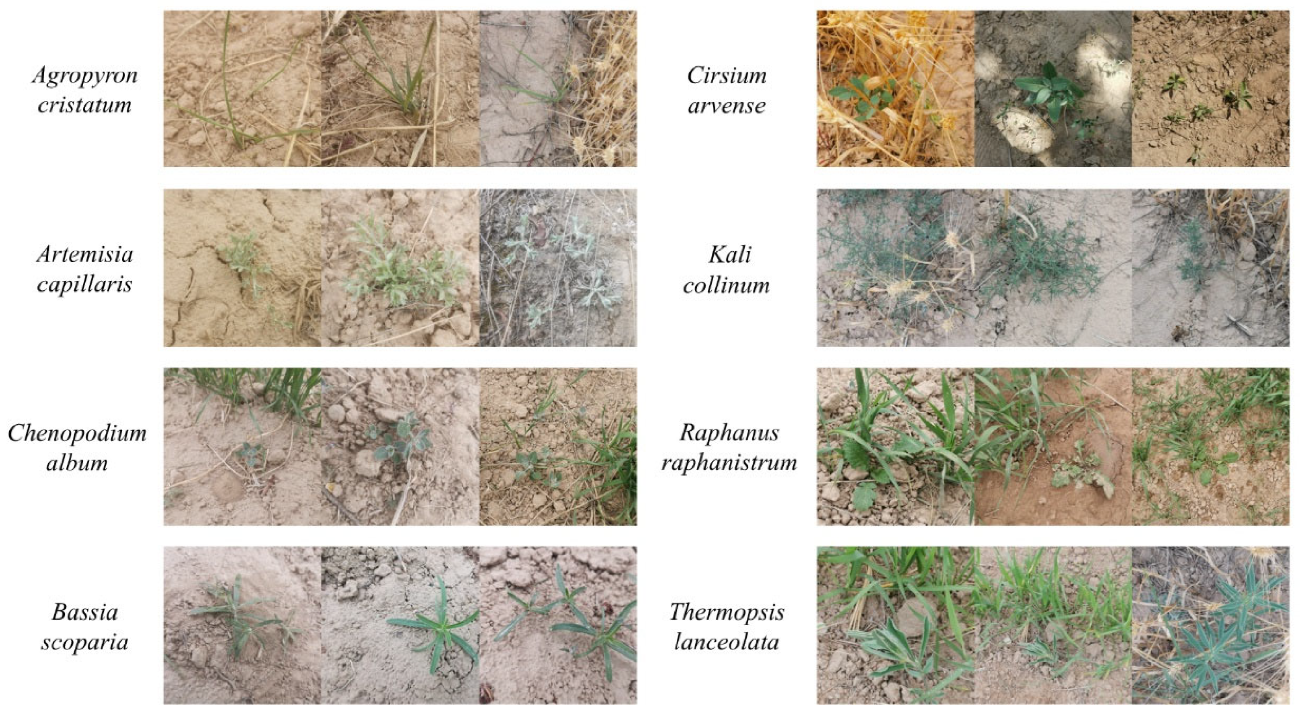
As shown in Figure 1, the dataset consists of 5967 images across eight well-balanced weed categories common in dryland spring wheat fields: Artemisia capillaris, Agropyron cristatum, Chenopodium album, Bassia scoparia, Cirsium arvense, Kali collinum, Raphanus raphanistrum, and Thermopsis lanceolata. These weed species were selected based on their high occurrence frequency and ecological significance in the local dryland farming systems. All images were captured using a smartphone with a 40-megapixel primary camera at a resolution of 2736 × 2736 pixels, from approximately 30–100 cm above ground level. Images were taken under various weather conditions (sunny, cloudy, and overcast) and from multiple angles to ensure environmental diversity and robust model training.

The dataset encompasses a wide range of weed density scenarios commonly encountered in dryland spring wheat fields, from sparse individual weed occurrences to high-density weed patches. This natural variation in weed density was deliberately captured during data collection to reflect realistic field conditions, including early-season sparse emergence patterns, localized weed clusters around field margins, and areas with varying degrees of weed competition intensity.

Ground truth annotations were created using Labelme (version 3.16.7) software with bounding box format and rectangular coordinates for each weed instance, and all annotations were validated by agricultural experts to ensure taxonomic accuracy. For this study, we specifically focused on the challenges of detecting and identifying these weed species in the complex backgrounds of dryland spring wheat fields. The dataset was split into training (4200 images), validation (600 images), and testing (1167 images) sets, with a ratio of approximately 7:1:2. The detailed annotation process and data augmentation techniques used to balance class distribution have been described in our previous work.

2.2. Experimental Tools, Training Parameters, and Environment

All experiments were conducted on a high-performance computing platform equipped with an NVIDIA RTX 4090 GPU featuring 24 GB of VRAM. The system utilized a 12 vCPU Intel Xeon Platinum 8352 V processor running at 2.10 GHz, complemented by 90 GB of system memory. The software environment consisted of Python 3.12, PyTorch 2.3.0, and CUDA 12.1. This computational setup provided sufficient resources for the training and evaluation of our lightweight YOLOv8-based model for weed detection in dryland spring wheat fields.

The training configuration was carefully optimized to ensure model convergence and fair comparison with baseline methods. The model was trained for 300 epochs, which was determined through preliminary experiments to guarantee sufficient convergence while preventing overfitting. Stochastic Gradient Descent (SGD) was employed as the optimizer with an initial learning rate of 0.001, selected based on empirical validation to balance convergence speed and training stability. The batch size was set to 64 to ensure efficient GPU memory utilization and stable gradient updates. All input images were resized to 640 × 640 pixels, maintaining consistency with the default configuration of the baseline YOLOv8 model to enable fair performance comparison.

2.3. Evaluation Metrics

Following Chen et al. [29], this study employs the following evaluation metrics: mean Average Precision (mAP, %), parameters (millions), model size (MB), GFLOPs (billions of floating-point operations per forward pass), and frames per second (FPS). These metrics provide a comprehensive assessment of both detection accuracy and computational efficiency, which are essential considerations for deploying weed detection systems in dryland spring wheat fields.

(1)

mAP (%): Mean Average Precision, which measures the detection accuracy across different classes and IoU thresholds. Higher mAP values indicate better detection performance.

(2)

Parameters (M): The total number of learnable parameters in the model, measured in millions. This metric reflects the model complexity and memory requirements.

(3)

Model Size (MB): The storage size of the model weights file in megabytes, which is relevant for deployment on resource-constrained devices.

(4)

GFLOPs: Giga Floating Point Operations, measured as billions of floating-point operations required for a single forward pass through the network. This metric quantifies the computational complexity of the model.

(5)

FPS: Frames Per Second, indicating the processing speed of the model during inference. Higher FPS values reflect better real-time detection capabilities, which is crucial for practical field applications.

2.4. YOLOv8

YOLOv8, released by Ultralytics in early 2023, represents the latest advancement in the YOLO series of object detection frameworks. It maintains the single-stage detection architecture while introducing several key innovations that enhance both performance and efficiency. The architecture utilizes an enhanced CSPDarknet backbone featuring optimized C2f modules for efficient feature extraction, combined with a modified PANet [30] structure for hierarchical feature fusion. Most notably, YOLOv8 abandons the anchor-based detection paradigm in favor of an anchor-free approach with decoupled classification and regression branches, significantly improving detection accuracy, especially for small objects.

Technical Features of YOLOv8:

(1)

Backbone Architecture: YOLOv8 employs an improved CSPDarknet backbone with C2f (Cross Stage Partial with 2 convolutions) modules that replace the C3 modules in YOLOv5. The C2f module enhances gradient flow and feature representation through additional skip connections and reduced computational overhead.

(2)

Neck Design: The neck utilizes a modified PANet structure with top-down and bottom-up feature pyramid networks (FPNs) for multi-scale feature fusion. The SPPF (Spatial Pyramid Pooling Fast) module efficiently captures multi-scale contextual information.

(3)

Anchor-free Detection Head: Unlike previous YOLO versions, YOLOv8 implements an anchor-free detection paradigm with decoupled classification and regression heads. This design reduces the number of box predictions per cell and improves localization accuracy for small objects.

(4)

Loss Functions: YOLOv8 integrates Distribution Focal Loss (DFL) for bounding box regression and Binary Cross Entropy (BCE) for classification, combined with Complete IoU (CIoU) loss for improved convergence and accuracy.

(5)

Data Augmentation: Advanced augmentation strategies, including Mosaic, MixUp, and adaptive anchor assignment during training, enhance model robustness and generalization capability.

YOLOv8 is available in five standard configurations of varying sizes: YOLOv8n, YOLOv8s, YOLOv8m, YOLOv8l, and YOLOv8x, which differ in network width (number of channels) and depth (number of layers). These configurations offer a range of options for balancing detection accuracy and computational efficiency based on specific application requirements. For our lightweight weed detection model for dryland spring wheat fields, we selected the YOLOv8n variant as our base architecture due to its smaller model size and faster inference speed, which are crucial for real-time detection applications in resource-constrained agricultural environments.

2.5. HSG-Net

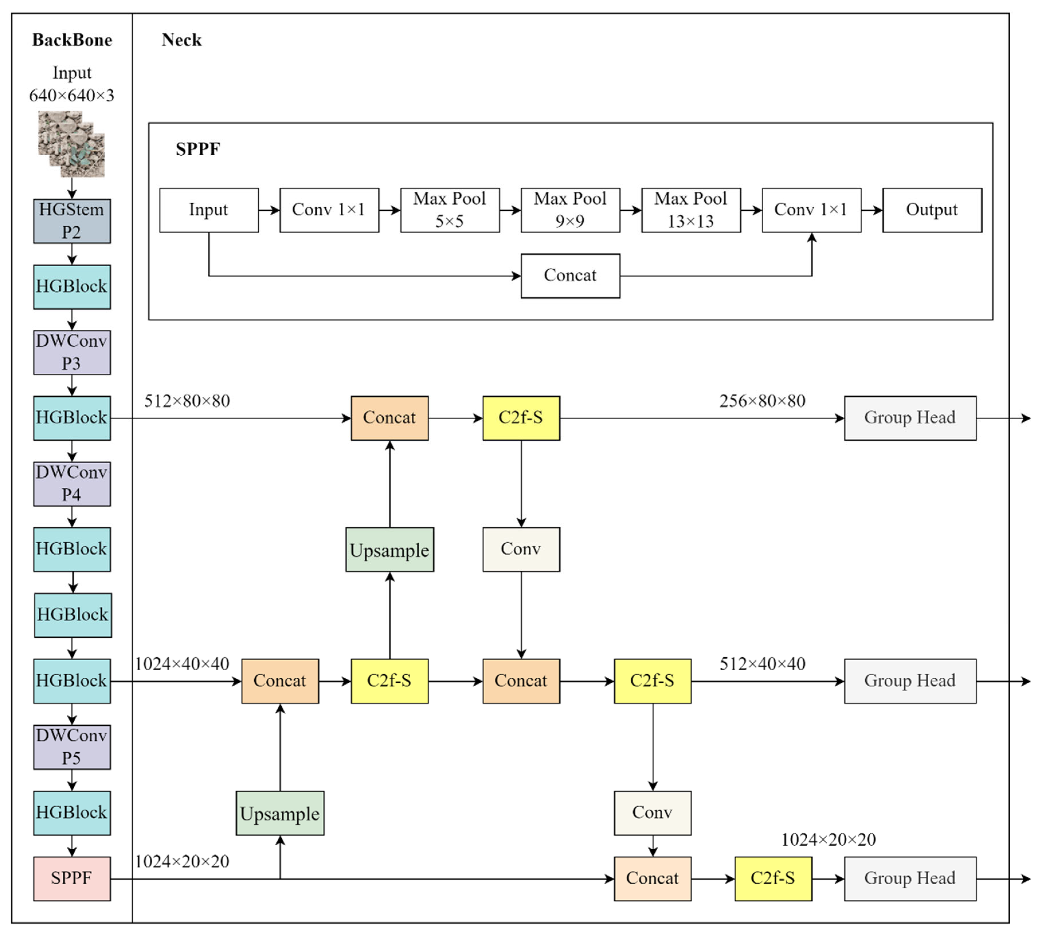
As illustrated in Figure 2, HSG-Net consists of three primary components: a backbone network based on HGNetv2, a neck structure with improved C2f-S modules, and custom lightweight Group Head detection heads.

The backbone of HSG-Net utilizes HGNetv2 from the RT-DETR [31] framework, replacing the conventional backbone of YOLOv8. The input image (640 × 640 × 3) is processed through a series of specialized layers, including HGStem, multiple HGBlock modules, and DWConv (P3, P4, P5) components arranged in a hierarchical structure. At the deepest level, an SPPF (Spatial Pyramid Pooling—Fast) module is incorporated to enhance the feature representation. This backbone extracts multi-scale features at three different resolutions: 1024 × 20 × 20, 1024 × 40 × 40, and 512 × 80 × 80.

The neck of the HSG-Net features our proposed C2f-S modules, which are improved versions of the C2f modules found in YOLOv8, inspired by the StarNet [32] architecture. These C2f-S modules efficiently fuse features from different scales through concatenation operations, with upsampling layers facilitating information flow from deeper to shallower layers. The network employs three C2f-S modules that progressively refine features and reduce dimensions from 1024 × 20 × 20 to 512 × 40 × 40 and finally to 256 × 80 × 80.

For the detection head, we designed a lightweight Group Head that employs two 3 × 3 grouped convolutions to efficiently process features while significantly reducing the parameter count. These Group Heads are deployed at three different scales to enable multi-scale detection, which is crucial for identifying weeds of varying sizes in complex agricultural environments.

2.5.1. HGNetv2 Backbone

The proposed model replaces the default YOLOv8 backbone with HGNetv2, a more efficient architecture originally developed for the RT-DETR framework. HGNetv2 is specifically designed for real-time object detection scenarios, offering an excellent balance between computational efficiency and feature representation capacity.

HGNetv2 consists of two primary components: the HGStem module and a series of HGBlock modules. The HGStem module serves as the network entry point, applying five convolutional operations and one max-pooling operation to efficiently reduce spatial dimensions while increasing channel depth.

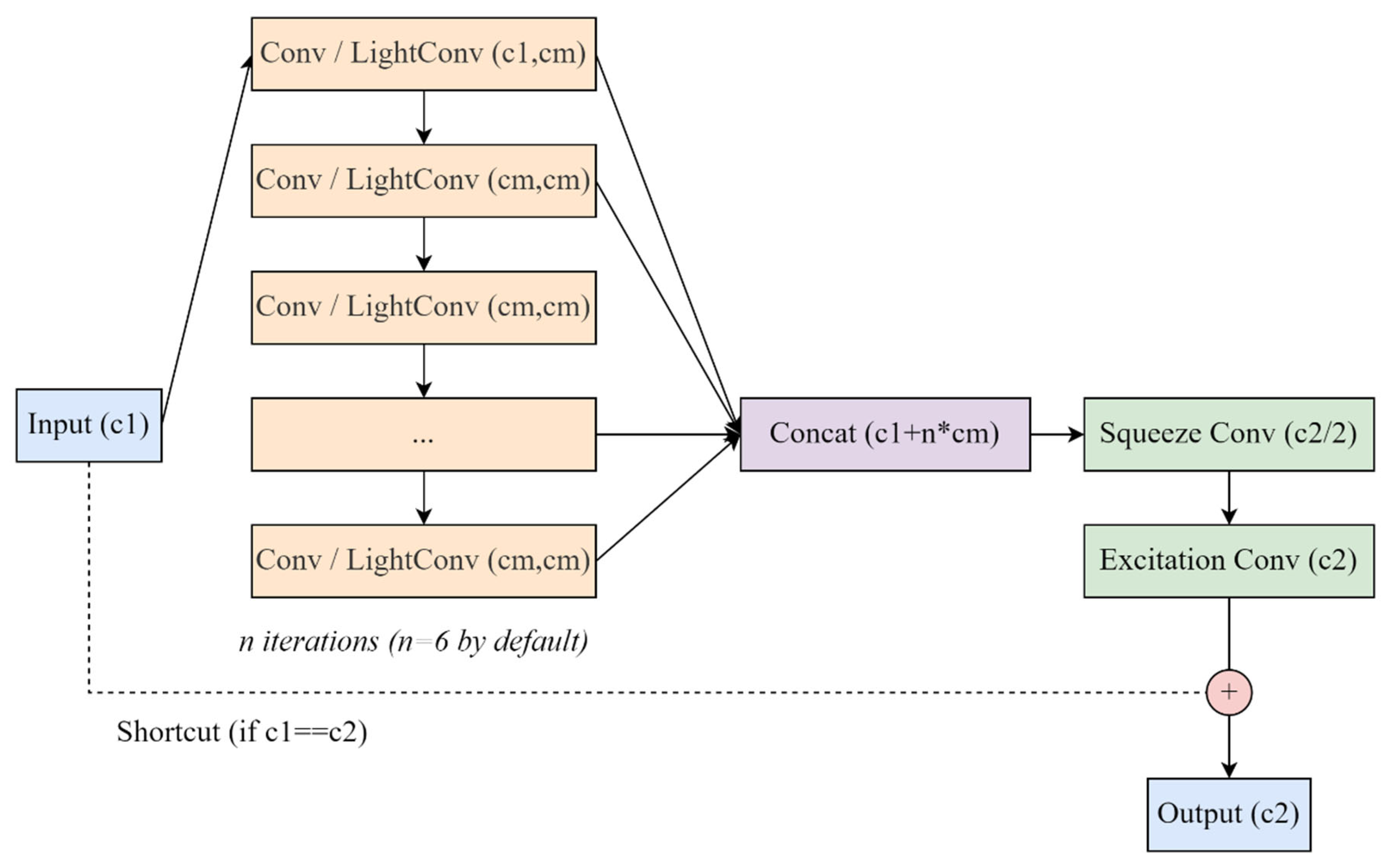
The HGBlock represents the core computational unit of HGNetv2, as illustrated in Figure 3. Its distinctive feature is a progressive feature accumulation approach that maintains a list of feature maps initialized with the input tensor itself. Rather than simply passing the input through sequential layers, HGBlock iteratively applies either standard Conv or LightConv operations to the most recently generated feature map, adding each new output to the feature list. This creates a hierarchical representation where each layer builds upon the previous one’s output.

After accumulating n processed feature maps (default n = 6), all features—including the original input—are concatenated along the channel dimension, resulting in a feature tensor with c1 + n × cm channels. This concatenated representation undergoes a two-stage dimensionality reduction process: first through a “squeeze” convolution (1 × 1) that reduces the channel count to c2/2, followed by an “excitation” convolution (1 × 1) that projects the features to the final output dimension c2. This squeeze-and-excitation mechanism enables the network to adaptively recalibrate feature responses by explicitly modeling interdependencies between channels.

Additionally, the HGBlock implements a conditional residual connection when the input and output dimensions match (c1 = c2). This shortcut connection adds the input directly to the processed features, facilitating gradient flow during training and enabling the construction of deeper networks. The combination of progressive feature accumulation, hierarchical representation learning, and adaptive feature recalibration makes HGBlock particularly effective for resource-constrained applications like real-time weed detection in agricultural settings.

2.5.2. C2f-S Module

To enhance feature extraction capabilities while maintaining computational efficiency, we adapted the Star structure from StarNet into our detection framework, proposing a C2f-S module as a replacement for the standard C2f module in YOLOv8. This adaptation introduces a star-shaped attention mechanism that leverages the powerful properties of element-wise multiplication operations in neural networks.

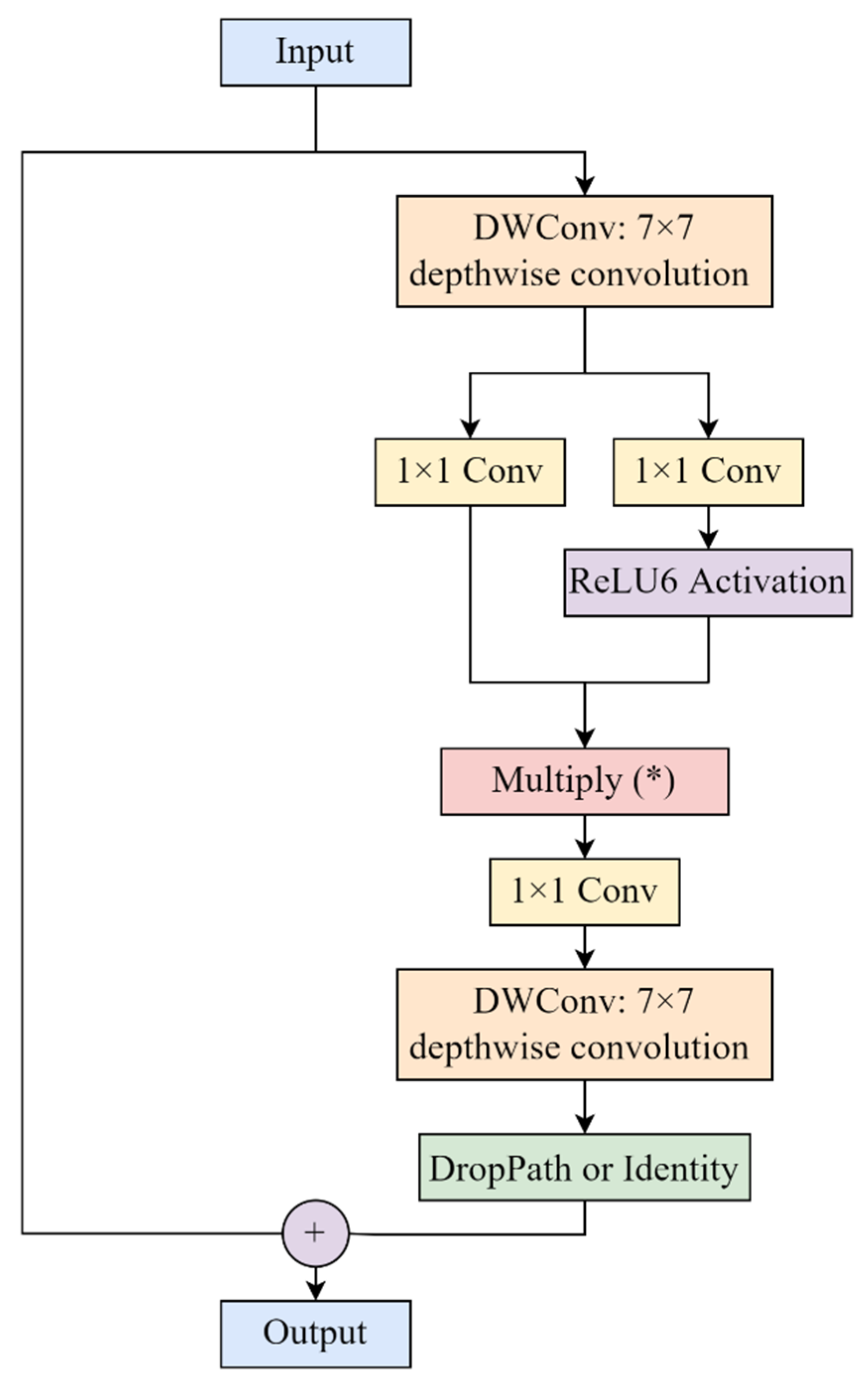
The C2f-S module inherits the basic structure of the C2f module but replaces the conventional bottleneck blocks with the adapted StarBlock. As illustrated in Figure 4, the StarBlock incorporates a specialized feature fusion mechanism that enables more effective feature extraction, particularly suited for detecting small weeds in complex agricultural environments.

The StarBlock begins with a 7 × 7 depthwise convolution that captures spatial information efficiently with minimal parameters. The output is then split into two parallel branches, both processed by 1 × 1 convolutions to expand the feature dimension. One branch undergoes ReLU6 activation [33], while the other remains unactivated. These branches are then multiplied element-wise, forming the core “star operation” of our module.

The star operation is mathematically defined by Equation (1):

$$\begin{array}{c}Z=\sigma \left(Z_1\right) \odot Z_2 \end{array}$$

(1)

where Z₁ and Z₂ represent the outputs of the two parallel 1 × 1 convolution branches, σ (·) denotes the ReLU6 activation function, and ⊙ represents element-wise multiplication. For any spatial location (i, j) and channel k, the operation is given by Equation (2):

$$\begin{array}{c}{Z}_{i,j,k}=max \left(0,min(6,Z_{1 i,j,k})\right)\times Z_{2 i,j,k}\end{array}$$

(2)

This star operation creates an efficient gating mechanism where the activated branch acts as learned attention weights for the unactivated branch, enabling the network to implicitly project features into a high-dimensional, non-linear feature space without increasing network width. The operation generates up to d² unique feature interactions through element-wise multiplication while maintaining linear computational complexity O (HWrd) and linear parameter scaling O (rd), where H and W denote the spatial dimensions, r represents the expansion ratio, and d is the feature dimension. This makes the star operation significantly more efficient than traditional attention mechanisms.

By integrating this star structure into the YOLOv8 architecture, we stack multiple Star_Blocks sequentially in the C2f-S module, with the number of blocks determined by the parameter n. The parameter n (number of StarBlocks) was empirically determined through preliminary experiments testing values of n ∈ {1, 2, 3, 4}. We found that n = 2 provided the optimal balance between feature representation capacity and computational efficiency, with n = 1 showing insufficient feature extraction capability and n ≥ 3 introducing computational overhead without significant accuracy improvements. This configuration maintains consistency with the original YOLOv8 C2f module structure while enhancing feature selectivity through the star operation.

This architecture enables hierarchical feature extraction while maintaining efficiency through the use of depthwise separable convolutions and the attention mechanism.

Compared to the original C2f module in YOLOv8, our adapted C2f-S offers several advantages:

(1)

Enhanced feature representation: The star operation maps inputs into a high-dimensional, non-linear feature space implicitly, similar to kernel methods but without computational overhead.

Improved feature selectivity: The multiplication operation after split branches acts as an adaptive feature selector, emphasizing relevant features while suppressing irrelevant ones.

(2)

Parameter efficiency: Despite the added representational capacity, the use of depthwise convolutions keeps the parameter count and computational requirements manageable.

(3)

Improved gradient flow: The residual connection facilitates better gradient propagation during backpropagation.

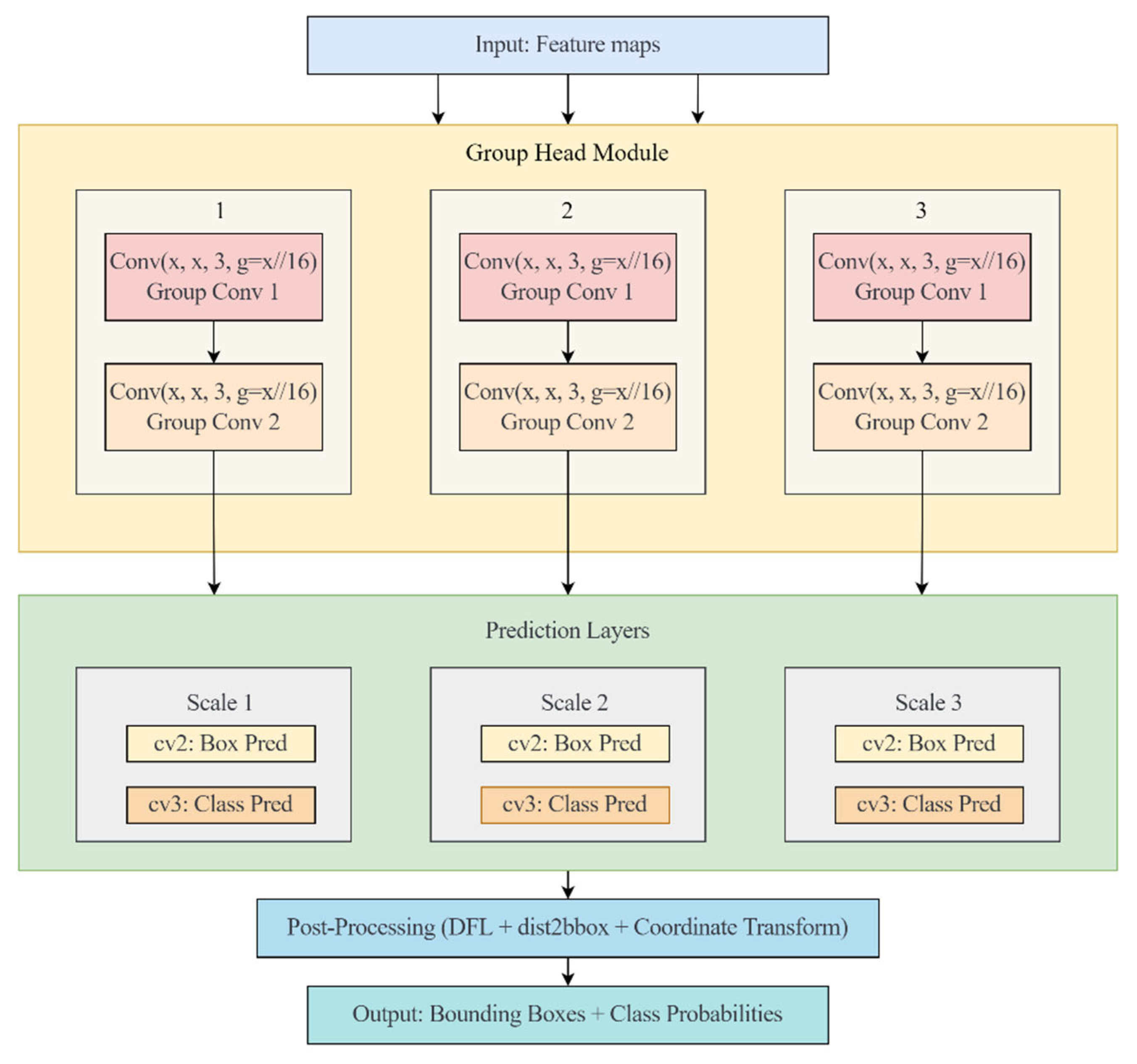
2.5.3. Group Head Module

As shown in Figure 5, our proposed Group Head Module consists of a multi-scale detection architecture that processes feature maps from the backbone network through specialized group convolution operations. The figure illustrates the complete detection pathway from input feature maps to final detection outputs.

At the top of Figure 5, the input feature maps from the backbone network enter the Group Head Module. These feature maps capture hierarchical representations at different scales, providing multi-scale information critical for detecting weeds of varying sizes in wheat fields. The feature maps are processed through three parallel branches (labeled as 1, 2, and 3 in Figure 5), each corresponding to a different scale.

Within each scale branch, the Group Head Module applies two consecutive group convolution operations. Each group convolution is configured with parameters Conv (x, x, 3, g = x/16), where

(1)

The first x represents the number of input channels at that specific scale.

(2)

The second x indicates that the output channel count matches the input.

(3)

The value 3 denotes the 3 × 3 kernel size.

(4)

The parameter g = x/16 indicates that the convolution channels are divided into x/16 groups.

The group size ratio of 16 was selected based on empirical evaluation of different ratios {4, 8, 16, 32}. Through preliminary experiments, we observed that g = x/16 achieved the best trade-off between parameter reduction and detection accuracy. Smaller ratios (g = x/4, g = x/8) maintained higher accuracy but with limited parameter reduction, while larger ratios (g = x/32) resulted in excessive parameter reduction that compromised detection performance, particularly for small weed targets.

The first group convolution (Group Conv 1) processes the input feature map by dividing the channels into groups, with each group processed independently. This operation significantly reduces the computational complexity compared to standard convolutions while preserving the spatial information necessary for accurate detection. The output from Group Conv 1 is then fed into Group Conv 2, which follows the same grouping strategy to further process the features while maintaining computational efficiency.

After processing through the Group Head Module, the feature maps from each scale branch flow into the Prediction Layers section. As illustrated in Figure 5, each scale branch splits into two parallel prediction paths:

(1)

Box Prediction (cv2): This path specializes in predicting the spatial coordinates of potential weed bounding boxes.

(2)

Class Prediction (cv3): This path focuses on determining the probability that the detected object belongs to a specific class (weed or background).

The outputs from all prediction layers then converge in the Post-Processing stage, which applies several operations:

(1)

Distribution Focal Loss (DFL) for refined coordinate prediction: DFL was selected over traditional regression losses due to its superior performance in handling the inherent uncertainty in bounding box coordinate prediction. Unlike conventional L1 or L2 losses that treat coordinate regression as point estimation, DFL models the coordinate prediction as a probability distribution, which is particularly beneficial for detecting small and irregularly shaped weed instances that are common in agricultural fields.

(2)

Distance-to-bounding-box transformation (dist2bbox) for converting relative coordinates to absolute bounding boxes: The dist2bbox transformation was chosen for its computational efficiency and numerical stability compared to direct coordinate regression. This method predicts the distances from anchor points to the four sides of bounding boxes, which naturally constrains the predictions to valid geometric configurations.

(3)

Coordinate transformation to align predictions with the input image dimensions: The Group Head module, which incorporates DFL and dist2bbox, significantly reduces computational complexity while maintaining competitive detection accuracy. Our comprehensive experiments comparing different backbone networks (

Table 1. Performance comparison of different backbone networks.

Backbone	mAP/%	Parameters/M	Model Size/MB	GFLOPs	FPS
YOLOv8n (baseline)	83.6	3.0	6.3	8.1	185.2
Vanillanet	82.9	24.0	59.8	96.7	105.3
UniRepLKNet	82.4	6.1	13.1	15.6	129.9
FasterNet	82.4	4.2	8.6	10.7	217.4
EfficientViT	81.9	4.0	8.8	9.4	185.2
Convnextv2	80.7	5.7	11.6	14.1	161.3
HGNetv2	82.9	2.4	5.0	6.9	208.3

) and object detection models (

Table 2. Performance comparison of different object detection models.

Model	mAP/%	Parameters/M	Model Size/MB	GFLOPs	FPS
YOLOv8n (baseline)	83.6	3.0	6.3	8.1	185.2
YOLOv8s	83.8	11.1	21.5	28.6	165.1
YOLOv8m	83.9	26.0	50.0	78.9	118.2
YOLOv8l	84.0	43.7	83.7	165.1	105.3
YOLOv8x	83.9	68.2	132.0	257.9	67.5
YOLOv5n	83.9	2.5	5.3	7.1	238.1
YOLOv10n	83.2	2.3	5.8	6.5	212.8
YOLOv11n	83.5	2.6	5.4	6.5	220.1
ATSS	83.8	32.1	245.5	126.0	45.5
RT-DETR-L	80.4	28.5	59.1	100.6	163.9
RetinaNet	84.4	36.5	278.5	130.0	54.2
Faster-RCNN	80.8	41.4	319.5	134.0	64.4
TOOD	81.9	32.0	246.8	124.0	33.5
HSG-Net	84.1	1.6	3.4	4.1	178.6

) demonstrate the effectiveness of our architectural choices. As evidenced in ablation studies (

Table 3. Ablation experiments.

Experiment Number	HGNetv2	C2f-S	Group Head	mAP/%	Parameters/M	Model Size/MB	GFLOPs	FPS
1	✕	✕	✕	83.6	3.0	6.3	8.1	185.2
2	✓	✕	✕	82.9	2.4	5.0	6.9	208.3
3	✕	✓	✕	82.9	2.5	5.4	6.9	217.4
4	✕	✕	✓	83.1	2.4	5.1	5.6	270.3
5	✓	✓	✕	83.1	2.2	4.6	6.5	344.8
6	✕	✓	✓	82.9	1.9	4.2	4.4	294.1
7	✓	✕	✓	82.6	1.8	3.7	4.5	263.2
8	✓	✓	✓	84.1	1.6	3.4	4.1	178.6

Note: ✓, use the improvement; ✕, do not use this improvement.

, Experiment 4), the Group Head alone achieves 83.1% mAP with only 2.4 M parameters and 5.6 GFLOPs, compared to the baseline’s 83.6% mAP with 3.0 M parameters and 8.1 GFLOPs. This demonstrates that the Group Head’s post-processing techniques (DFL and dist2bbox) effectively preserve detection performance while reducing model complexity. Furthermore, when integrated with the HGNetv2 backbone and C2f-S modules (Table 3, Experiment 8), the complete HSG-Net model achieves 84.1% mAP, outperforming the baseline by 0.5%. This synergistic improvement confirms the value of DFL and dist2bbox for precise boundary delineation in weed detection, particularly for distinguishing small weed targets from complex soil and crop backgrounds during early growth stages in dryland spring wheat fields.

The final output, as shown at the bottom of Figure 5, consists of precise bounding boxes with associated class probabilities, enabling accurate weed detection and localization in wheat fields.

3. Results and Analysis

3.1. Model Performance Comparison

As shown in Table 1, we compared various backbone networks for weed detection in dryland spring wheat fields, including YOLOv8n (baseline), VanillaNet [34], UniRepLKNet [35], FasterNet [36], EfficientViT [37], Convnextv2 [38], and HGNetv2. The baseline YOLOv8 model demonstrated the highest mean Average Precision (mAP) at 83.6%, but with moderate computational demands (8.1 GFLOPs) and model size (6.3 MB). Among the alternatives evaluated, HGNetv2 stands out as particularly promising, achieving a competitive mAP of 82.9% while requiring only 2.4 million parameters—significantly fewer than any other tested backbone. This translates to the smallest model size (5.0 MB) and lowest computational cost (6.9 GFLOPs) among all tested networks.

The lightweight nature of HGNetv2 does not substantially compromise detection performance, with its mAP only 0.7% lower than the baseline while reducing parameter count by approximately 20%. Moreover, HGNetv2 achieves impressive inference speed (208.3 FPS), second only to FasterNet (217.4 FPS), making it highly suitable for real-time applications in agricultural settings.

Other backbone networks, such as VanillaNet, demonstrated comparable accuracy (82.9% mAP) but required substantially more parameters (24.0 M) and computational resources (96.7 GFLOPs), making them less suitable for deployment on resource-constrained devices commonly used in field conditions. Similarly, UniRepLKNet and FasterNet achieved reasonable accuracy but with higher computational demands than HGNetv2.

Based on the comprehensive evaluation of detection accuracy, model size, computational efficiency, and inference speed as presented in Table 1, we selected HGNetv2 as the backbone network for our lightweight YOLOv8-based weed detection model. This selection is justified by HGNetv2’s excellent balance of performance metrics: While experiencing only a modest 0.7% reduction in mAP compared to the baseline YOLOv8 (82.9% vs. 83.6%), HGNetv2 reduces parameter count by 20% (2.4 M vs. 3.0 M), model size by 20.6% (5.0 MB vs. 6.3 MB), and computational demands by 14.8% (6.9 GFLOPs vs. 8.1 GFLOPs). Furthermore, HGNetv2 achieves a 12.5% improvement in inference speed (208.3 FPS vs. 185.2 FPS) compared to the baseline.

As shown in Table 2, we evaluated various object detection models for weed detection in dryland spring wheat fields, including YOLOv8 (various variants), YOLOv5n, YOLOv10n [39], YOLOV11n [40], ATSS [41], RT-DETR-L [31], RetinaNet [42], Faster-RCNN [43], TOOD [44], and our proposed HSG-Net. The comparison reveals that RetinaNet achieved the highest mean Average Precision (mAP) at 84.4%, but at the significant cost of large model size (278.5 MB) and high computational demands (130.0 GFLOPs), resulting in relatively low inference speed (54.2 FPS).

Our proposed HSG-Net demonstrated excellent performance with an mAP of 84.1%, only 0.3% lower than RetinaNet, while requiring drastically fewer parameters (1.6 M) and computational resources (4.1 GFLOPs). This makes HSG-Net the most lightweight model among all tested architectures, with a model size of just 3.4 MB—approximately 98% smaller than RetinaNet and 46% smaller than YOLOv5n, which was the second most compact model.

The YOLO family models demonstrated strong performance across different architectural scales. Among the YOLOv8 variants, YOLOv8n achieved 83.6% mAP with 3.0 M parameters, while larger variants (YOLOv8s, YOLOv8m, YOLOv8l, YOLOv8x) showed marginal improvements in accuracy (83.8–84.0% mAP) at the cost of substantially increased computational demands (11.1 M–68.2 M parameters) and reduced inference speeds (67.5–165.1 FPS). Based on this comparison, YOLOv8n was selected as our baseline model due to its optimal balance between detection accuracy and computational efficiency, providing only 0.2–0.4% lower mAP than larger variants while requiring significantly fewer resources, making it most suitable for lightweight optimization in resource-constrained agricultural environments. The lightweight YOLO variants (YOLOv5n, YOLOv10n, YOLOv11n) achieved comparable performance with mAP values ranging from 83.2% to 83.9% and maintained good inference speeds between 212.8 and 238.1 FPS. However, HSG-Net achieved superior detection accuracy (84.1% mAP) while requiring significantly fewer parameters (1.6 M) and computational resources than all tested YOLO variants, demonstrating an optimal balance between accuracy and efficiency for resource-constrained agricultural applications.

Traditional two-stage detectors, such as Faster-RCNN and single-stage models like ATSS and TOOD, demonstrated reasonable detection performance but were substantially heavier in terms of parameters (32.0–41.4 M) and model size (245.5–319.5 MB), making them less suitable for deployment in resource-constrained agricultural environments. Additionally, their inference speeds (33.5–64.4 FPS) were considerably lower than those of the YOLO family models and our HSG-Net.

Based on the comprehensive evaluation presented in Table 2, HSG-Net emerges as the optimal choice for weed detection in dryland spring wheat fields. Compared to the baseline YOLOv8n model, HSG-Net achieves a 0.5% higher mAP (84.1% vs. 83.6%) while reducing the parameter count by 46.7% (1.6 M vs. 3.0 M), model size by 46.0% (3.4 MB vs. 6.3 MB), and computational complexity by 49.4% (4.1 GFLOPs vs. 8.1 GFLOPs). Although HSG-Net’s inference speed (178.6 FPS) is slightly lower than YOLOv8n’s (185.2 FPS), representing a 3.6% reduction, this minor trade-off in speed is well justified by the substantial improvements in model efficiency and detection accuracy.

3.2. Ablation Study

As shown in Table 3, we conducted comprehensive ablation experiments to evaluate the individual and combined contributions of three key components in our proposed weed detection model: HGNetv2 backbone, C2f-S module, and Group Head detection head.

Experiment 1 represents the baseline YOLOv8n model without any of our proposed improvements, achieving an mAP of 83.6% with 3.0 M parameters and 8.1 GFLOPs. In Experiments 2–4, we individually incorporated each component to assess its separate contributions. Integrating only HGNetv2 (Experiment 2) reduced parameters by 20% (2.4 M vs. 3.0 M) and GFLOPs by 14.8% (6.9 vs. 8.1) while maintaining competitive accuracy (82.9% mAP). Similarly, incorporating only C2f-S (Experiment 3) achieved comparable accuracy with a significant reduction in computational demands. The Group Head detection head alone (Experiment 4) improved the inference speed substantially to 270.3 FPS (45.9% increase from baseline) while reducing computational complexity by 30.9% (5.6 vs. 8.1 GFLOPs).

Experiments 5–7 explored binary combinations of these components. The combination of HGNetv2 with C2f-S (Experiment 5) yielded impressive results with a slight improvement in mAP (83.1%) and remarkable gains in inference speed (344.8 FPS, 86.2% faster than baseline). The C2f-S and Group Head detection head combination (Experiment 6) achieved a significant reduction in computational complexity (4.4 GFLOPs, 45.7% lower than baseline). However, the HGNetv2 and Group Head detection head combination (Experiment 7) showed a slight decrease in mAP to 82.6% despite substantial improvements in model efficiency (1.8 M parameters, 4.5 GFLOPs).

Notably, Experiment 8, which incorporates all three proposed components (HGNetv2 backbone, C2f-S module, and Group Head detection head), demonstrated the best overall performance with an mAP of 84.1% (0.5% higher than baseline) while requiring only 1.6 M parameters (46.7% reduction), 3.4 MB model size (46.0% reduction), and 4.1 GFLOPs (49.4% reduction). Although the inference speed (178.6 FPS) is slightly lower than some other configurations, the substantial improvements in detection accuracy and model efficiency clearly demonstrate the complementary benefits of integrating all three components, resulting in our final HSG-Net model that achieves an optimal balance between accuracy and resource efficiency for real-time weed detection in dryland spring wheat fields.

Component-Wise Analysis

HGNetv2 Backbone: Reduces parameters by 20% (2.4 M vs. 3.0 M) while maintaining competitive accuracy (82.9% mAP). The progressive feature accumulation enables efficient hierarchical learning but causes 0.7% mAP reduction due to lightweight design trade-offs.

C2f-S Module: The star-shaped attention creates d² feature interactions with linear complexity O (HWrd), enhancing feature selectivity for small weed detection. However, the 7 × 7 depthwise convolution increases memory consumption.

Group Head: Dramatically improves inference speed (270.3 FPS vs. 185.2 FPS) while reducing parameters. The channel grouping limits inter-group information exchange but maintains detection accuracy through parallel processing.

Synergistic Effects: Combined implementation (84.1% mAP) outperforms individual components, demonstrating complementary advantages where HGNetv2’s efficiency, C2f-S’s representation enhancement, and Group Head’s lightweight detection work cooperatively.

3.3. Confusion Matrix Analysis

Figure 6 displays the normalized confusion matrices of the baseline YOLOv8n and our proposed HSG-Net models, providing a detailed visualization of classification performance across eight weed species and the background class. Each row in the matrices represents the predicted class, while each column represents the actual class. The diagonal elements indicate the proportion of correctly classified instances, with higher values (darker blue) signifying better classification performance.

The comparison reveals that HSG-Net demonstrates improvements in classification accuracy for most weed species compared to the baseline YOLOv8n model. For Artemisia, HSG-Net achieves a higher accuracy of 0.81 compared to YOLOv8n’s 0.80, indicating a slight improvement in detection performance. Similarly, for Agropyron, HSG-Net reaches 0.57 versus YOLOv8n’s 0.53, representing a 7.5% increase in classification accuracy.

Significant improvement is observed for Chenopodium, where HSG-Net achieves 0.64 compared to YOLOv8n’s 0.62, and for Bassia, with HSG-Net reaching 0.76 versus YOLOv8n’s 0.73. These improvements are particularly valuable considering that these species often share visual characteristics with other plants in dryland spring wheat fields, making them challenging to distinguish.

For Cirsium, both models perform equally well with an accuracy of 0.89. However, HSG-Net outperforms YOLOv8n for Kali, achieving 0.91 compared to 0.89, representing a 2.2% improvement. For Thermopsis, HSG-Net slightly outperforms the baseline with an accuracy of 0.93 versus 0.92.

It is worth noting that HSG-Net shows a slight decrease in performance for Raphanus (0.84 versus 0.85 in YOLOv8n). This minor reduction might be attributed to the model’s lighter architecture, which may occasionally compromise the detection of certain features specific to Raphanus.

Regarding misclassifications, both models show similar patterns, with the most frequent confusion occurring between weed species and the background class. For instance, YOLOv8n misclassifies 25% of Chenopodium and 25% of Raphanus instances as background, while HSG-Net misclassifies 28% of Chenopodium and 17% of Raphanus as background. This indicates that HSG-Net has significantly improved in distinguishing Raphanus from the background, reducing misclassification by 8 percentage points.

The background class itself shows notable differences in misclassification patterns. YOLOv8n most frequently confuses the background with Agropyron (47%) and Chenopodium (33%), while HSG-Net reduces these misclassifications to 43% and 28%, respectively. This improvement suggests that HSG-Net’s architectural modifications enhance its ability to distinguish actual weeds from complex field backgrounds.

The confusion matrix analysis demonstrates that despite its significantly reduced parameter count and computational requirements (1.6 M parameters and 4.1 GFLOPs versus YOLOv8n’s 3.0 M parameters and 8.1 GFLOPs), HSG-Net maintains and even improves classification accuracy for most weed species.

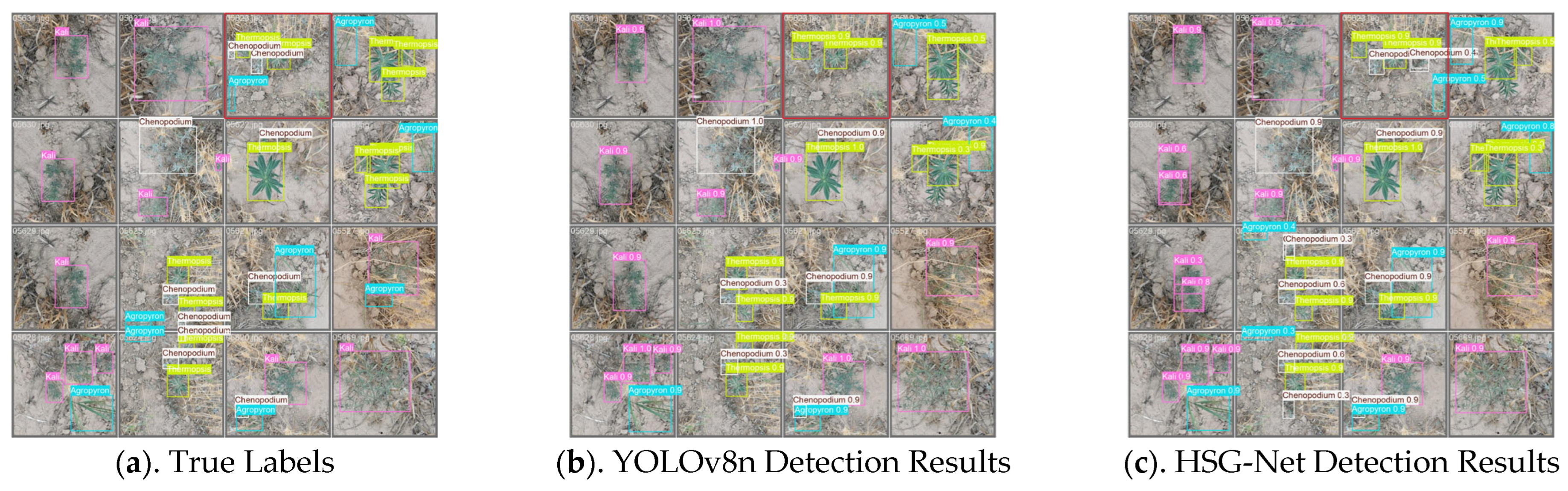
3.4. Visualization of Model Detection Results

Figure 7 presents a visual comparison of detection results from both the baseline YOLOv8n model and our proposed HSG-Net.

As highlighted by the red box in the third column of the first row of each sub-figure, HSG-Net successfully detects several small weed targets that YOLOv8n fails to identify. This demonstrates HSG-Net’s enhanced sensitivity to small-scale objects, which is particularly valuable for early-stage weed detection when plants are smaller and intervention is most effective.

The visualization results reveal several key performance characteristics of HSG-Net compared to the baseline model:

(1)

Enhanced small target detection: HSG-Net shows superior capability in detecting smaller weeds, as evidenced by the successful identification of small Thermopsis and Chenopodium specimens that YOLOv8n missed. This improved performance with small targets can be attributed to the architecture’s efficient feature extraction and the star-shaped attention mechanism in the C2f-S module, which enhances the model’s ability to capture fine-grained details.

(2)

Higher confidence scores: For many detected weeds, HSG-Net produces higher confidence scores than YOLOv8n. For example, in several instances of Kali detection, HSG-Net assigns confidence scores of 0.9–1.0, while YOLOv8n’s scores for the same targets are generally lower. This indicates HSG-Net’s improved certainty in its classifications despite having significantly fewer parameters.

(3)

Reduced false negatives: The visualizations show that HSG-Net reduces missed detections, particularly in complex scenes where weeds partially overlap or are partially obscured. This is evident in scenes containing multiple Thermopsis plants, where HSG-Net identifies more instances than YOLOv8n.

(4)

Consistent performance across species: HSG-Net maintains strong detection performance across all weed species in the test set, showing particular improvement in detecting Chenopodium and Thermopsis specimens compared to the baseline model.

(5)

Resilience to background complexity: The model demonstrates robust detection capability even against the complex and variable soil backgrounds typical of dryland spring wheat fields, where the visual distinction between plant material and soil can be subtle.

These visualization results align with our quantitative findings, confirming that HSG-Net’s architectural improvements translate to tangible detection enhancements in field conditions. The model’s ability to detect small weed targets with high confidence is particularly valuable for precision agriculture applications, where early and accurate weed identification enables timely, targeted interventions that can reduce herbicide use while maintaining effective weed control.

4. Discussion

The results demonstrate that the proposed HSG-Net model achieves an effective balance between detection accuracy and computational efficiency for weed detection in dryland spring wheat fields. This lightweight architecture slightly improves detection performance (84.1% mAP compared to the baseline YOLOv8n’s 83.6% mAP), while substantially reducing computational requirements—decreasing parameters by 46.7%, model size by 46.0%, and GFLOPs by 49.4%.

The integration of our three key components—HGNetv2 backbone, C2f-S modules with star-shaped attention mechanisms, and Group Head detection heads—creates synergistic effects that exceed the contributions of individual components. While each component independently reduces computational complexity with minimal impact on accuracy, their combination produces superior overall performance. This suggests that addressing different aspects of the detection pipeline in a coordinated manner is crucial for developing efficient yet accurate weed detection models.

The confusion matrix analysis reveals that HSG-Net demonstrates improved classification accuracy for 6 out of 8 weed species compared to the baseline model. Particularly notable are the improvements in detecting Chenopodium and Agropyron, which are challenging to identify in dryland spring wheat fields due to visual similarities with crops and complex backgrounds. The visualization results further confirm that HSG-Net enhances the detection of small weed targets with high confidence, addressing a critical need for early-stage detection when intervention is most effective.

Despite these promising results, several limitations should be acknowledged. First, the model evaluation was conducted on a dataset collected from a single geographical location (Anding District, Dingxi City, Gansu Province, China), which may limit its generalizability to other dryland wheat production regions with different weed species, soil conditions, and climate patterns. The transferability of HSG-Net to other agricultural ecosystems requires further investigation.

Second, although HSG-Net shows a slight reduction in inference speed (178.6 FPS versus YOLOv8n’s 185.2 FPS), the model’s performance under varying hardware constraints, particularly on embedded systems or mobile devices commonly used in field conditions, needs further examination. The current performance metrics were obtained using high-performance computing equipment (NVIDIA RTX 4090 GPU), which may not reflect the real-world performance on resource-constrained devices.

Third, while HSG-Net performs well across various growth stages and environmental conditions included in our dataset, its robustness to extreme weather conditions (heavy rain, strong wind, drought stress) or unusual lighting conditions (dawn, dusk, or overcast) may be limited by the diversity of the training data. The model’s performance consistency across these varying conditions requires further validation.

Finally, the current implementation does not address the practical integration challenges with automated weed control systems, such as precision spraying or mechanical removal. The end-to-end system performance, including detection accuracy, processing time, and control precision, needs evaluation in practical field operations to fully assess the model’s utility for sustainable weed management in dryland spring wheat production.

Addressing these limitations provides clear directions for future research to enhance the practical applicability and robustness of lightweight deep learning models like HSG-Net for weed detection in resource-constrained agricultural environments.

5. Conclusions

This study presents HSG-Net, a novel lightweight object detection model based on YOLOv8 for weed identification in dryland spring wheat fields. The model integrates three key innovations: an HGNetv2 backbone for efficient feature extraction, C2f-S modules with star-shaped attention mechanisms for enhanced feature representation, and Group Head detection heads for parameter-efficient prediction. Experimental results demonstrate that HSG-Net achieves superior detection accuracy (84.1% mAP) compared to the baseline YOLOv8n (83.6% mAP) while significantly reducing computational requirements—decreasing parameter count by 46.7% (1.6 M vs. 3.0 M), model size by 46.0% (3.4 MB vs. 6.3 MB), and computational complexity by 49.4% (4.1 GFLOPs vs. 8.1 GFLOPs).

Ablation studies confirm the complementary contributions of each architectural component, with their combination producing synergistic effects that enhance both efficiency and accuracy. Confusion matrix analysis reveals improved classification performance for 6 out of 8 weed species, particularly for Chenopodium and Agropyron, which are notoriously difficult to detect in dryland spring wheat fields. Visualization results further demonstrate HSG-Net’s enhanced capability to detect small weed targets with high confidence, which is crucial for early intervention in sustainable weed management.

The lightweight nature of HSG-Net makes it particularly suitable for deployment on resource-constrained devices used in precision agriculture, enabling real-time weed detection and targeted intervention in field conditions. This addresses a critical need in dryland spring wheat production systems, where efficient weed management is essential for optimizing limited water and nutrient resources.

Future research directions should focus on addressing the identified limitations. First, expanding the evaluation to diverse geographical regions with different soil conditions, climate patterns, and weed species would enhance the model’s generalizability. Second, the model’s performance on embedded systems and mobile devices commonly used in field conditions requires thorough examination to validate its real-world applicability. Third, testing HSG-Net’s robustness under extreme weather conditions and unusual lighting scenarios would improve its reliability in varied agricultural environments. Finally, evaluating the end-to-end system performance when integrated with automated weed control mechanisms would provide valuable insights into its practical utility for sustainable weed management in dryland spring wheat production.

By addressing these challenges, future work can enhance the practical applicability and robustness of lightweight deep learning models like HSG-Net for weed detection in resource-constrained agricultural environments, ultimately contributing to more sustainable and efficient weed management practices in dryland farming systems.