
Retrieval and Evaluation of NOX Emissions Based on a Machine Learning Model in Shandong


Abstract
1. Induction
2. Data and Methods
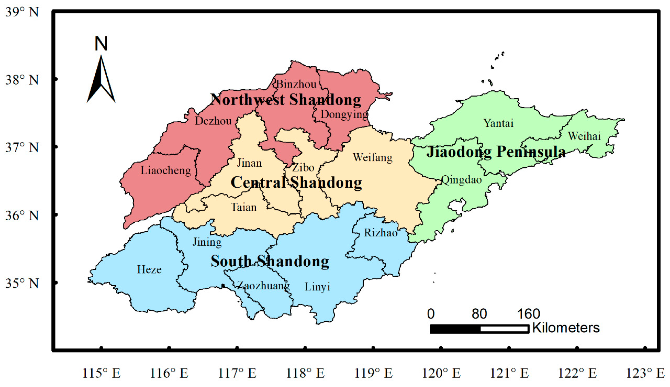
2.1. Study Area
2.2. NO2 Tropospheric Vertical Column Measurements
2.3. Meteorological Reanalysis Data
2.4. Prior Emissions
2.5. Machine Learning (ML) Model and Input Variables
2.5.1. WOA
2.5.2. XGBoost
2.5.3. WOA-XGBoost Modeling Procedure
- (1)
- The population and iteration times are initialized in the WOA algorithm, and the optimization range for each hyperparameter of XGBoost is set.
- (2)
- The training data is inputted into the XGBoost model, and the fitness of each whale individual in the population is computed based on the score of the respective XGBoost model regarding 10–fold cross–validation (CV) on the training dataset.
- (3)
- The position of each individual whale is updated, which provides a new set of hyperparameters.
- (4)
- Steps (2) and (3) are repeated iteratively until the termination criteria are satisfied. At the end of the iteration, WOA outputs the optimal whale position, which is the optimal hyperparameter for the XGBoost model.
- (5)
- The optimal hyperparameters are inputted into the XGBoost model for simulation, and its performance is evaluated.
2.5.4. Training Dataset for WOA-XGBoost
2.6. Model Evaluation Metrics
3. Results and Discussion
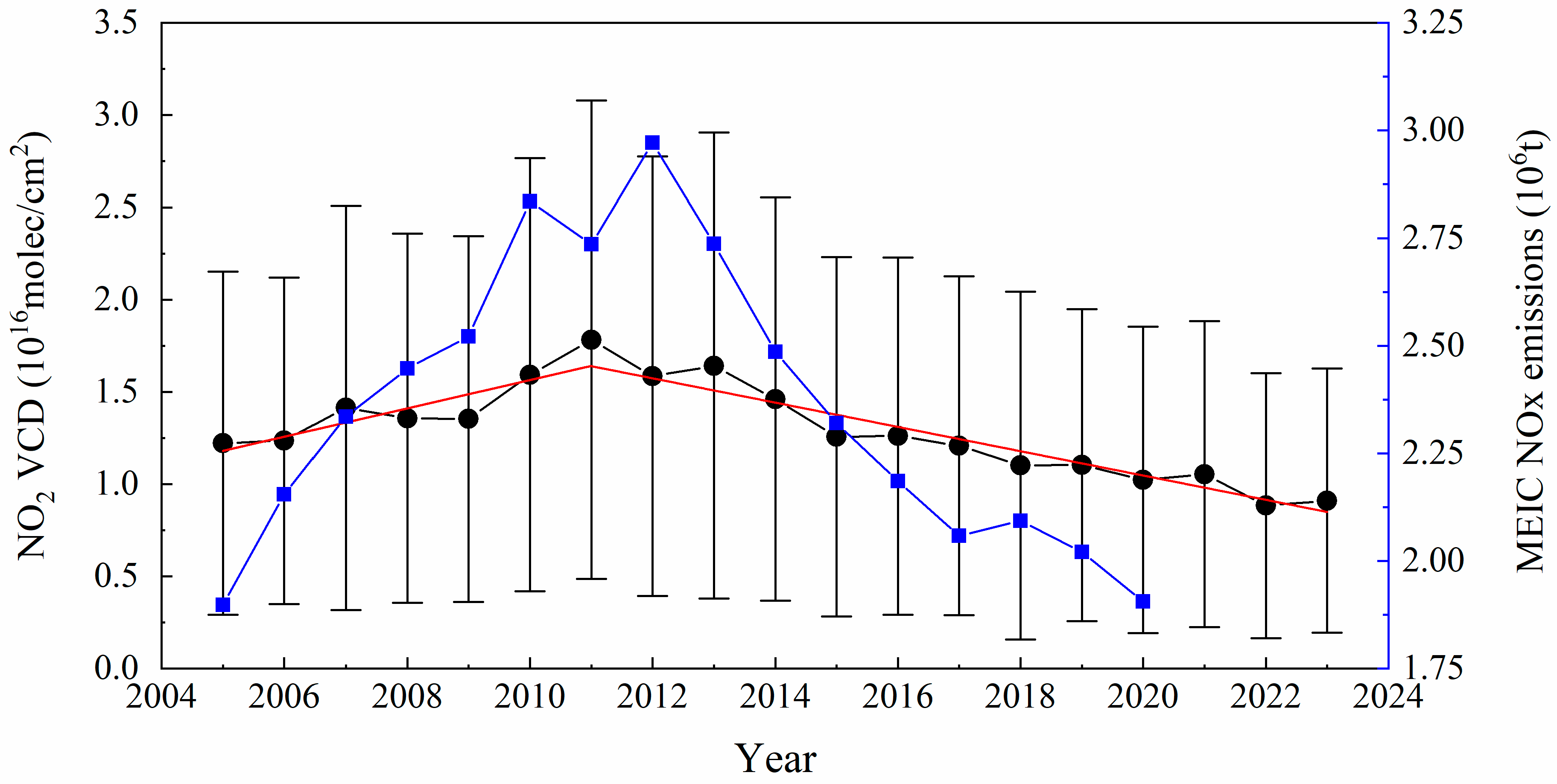
3.1. Variation in NO2 VCD and NOX Emissions in Shandong
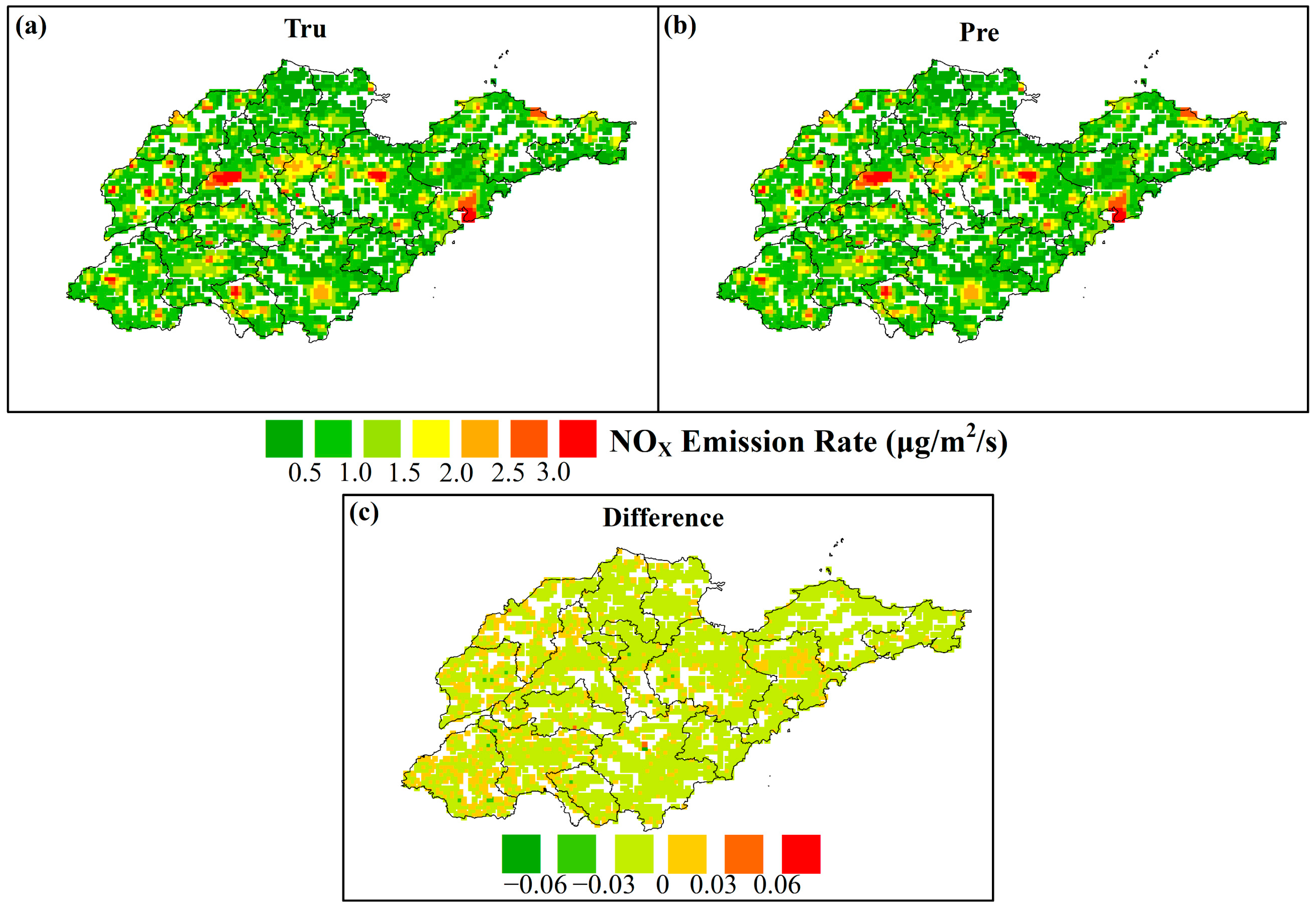
3.2. Evaluations for NOX Emission Rate Retrieval
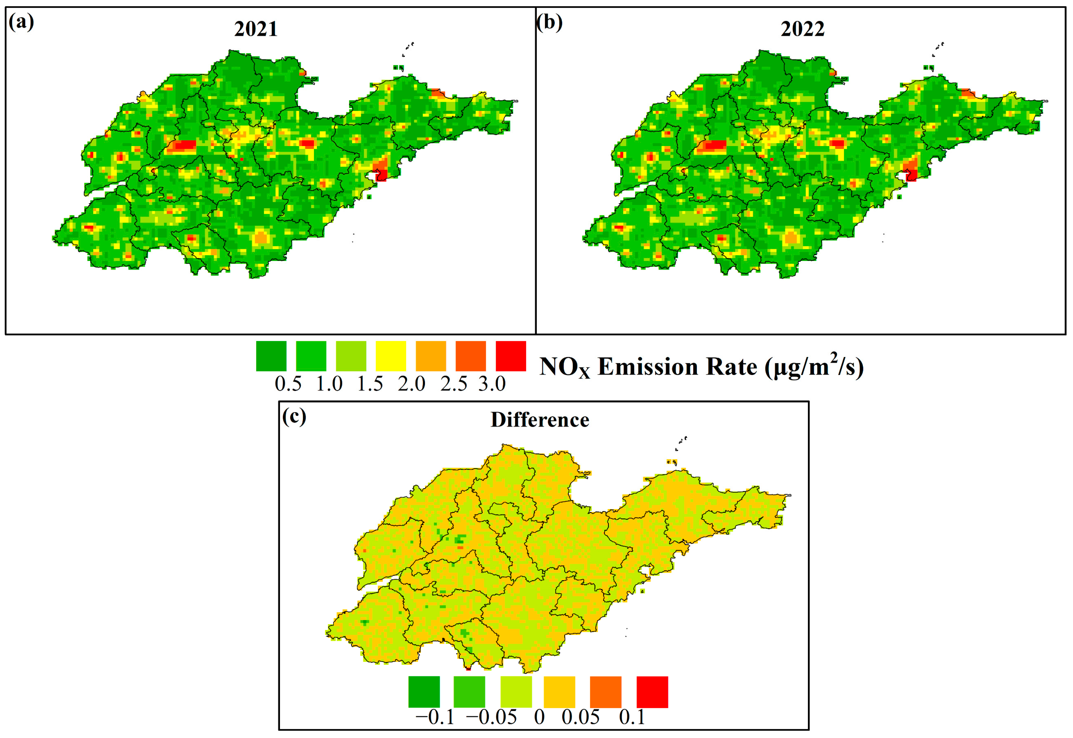
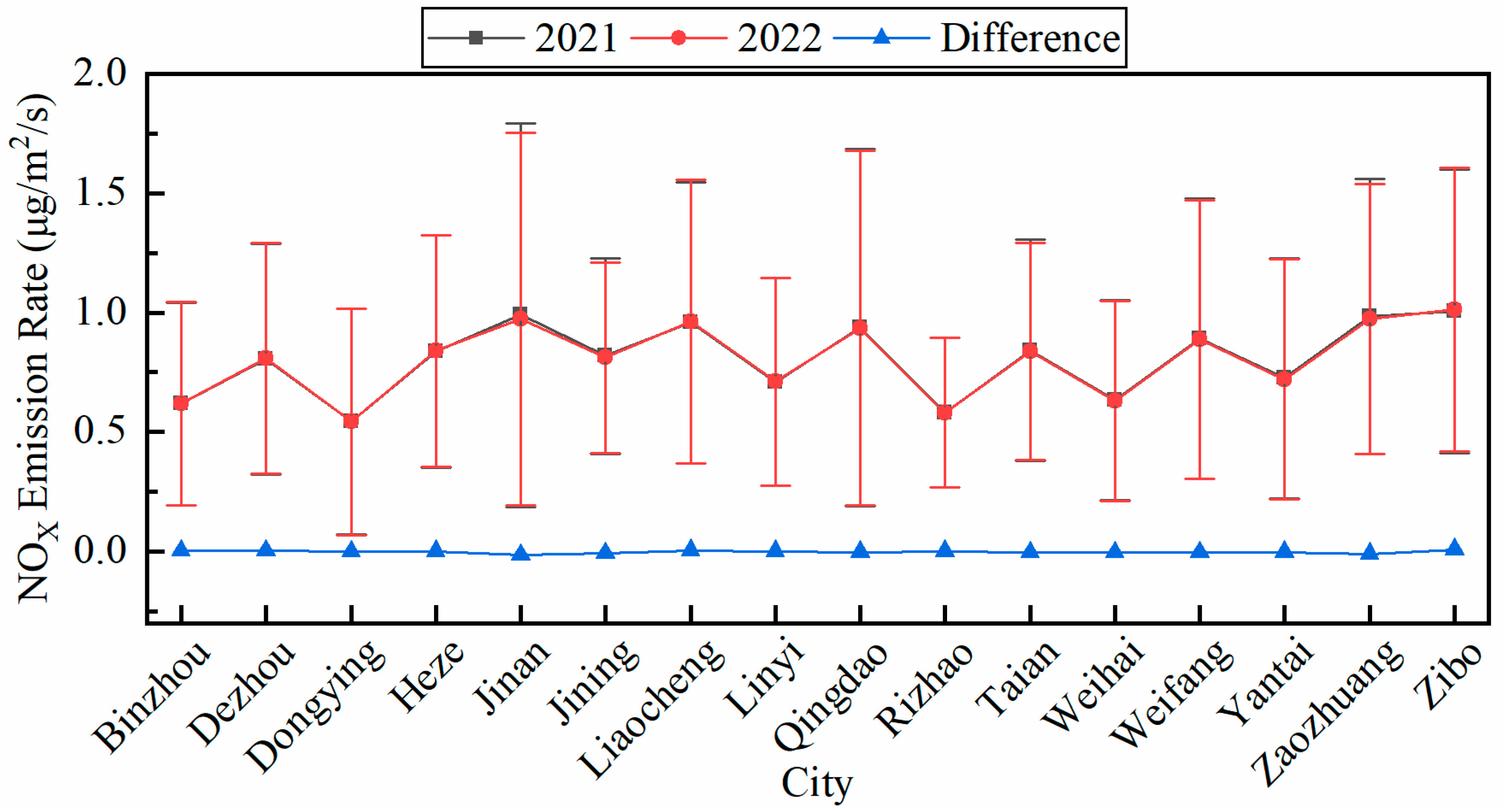
3.3. NOX Emission Rate Retrieval for 2021 and 2022
4. Conclusions
Supplementary Materials
Author Contributions
Funding
Institutional Review Board Statement
Informed Consent Statement
Data Availability Statement
Conflicts of Interest
References
- Shah, V.; Jacob, D.J.; Li, K.; Silvern, R.F.; Zhai, S.; Liu, M.; Lin, J.; Zhang, Q. Effect of changing NOX lifetime on the seasonality and long-term trends of satellite-observed tropospheric NO2 columns over China. Atmos. Chem. Phys. 2020, 20, 1483–1495. [Google Scholar] [CrossRef]
- Sun, W.; Shao, M.; Granier, C.; Liu, Y.; Ye, C.S.; Zheng, J.Y. Long-Term Trends of Anthropogenic SO2, CO, and NMVOCs Emissions in China. Earths Future 2018, 6, 1112–1133. [Google Scholar] [CrossRef]
- Ayazpour, Z.; Sun, K.; Zhang, R.; Shen, H. Evaluation of the Directional Derivative Approach for Timely and Accurate Satellite-Based Emission Estimation Using Chemical Transport Model Simulation of Nitrogen Oxides. J. Geophys. Res. Atmos. 2025, 130, e2024JD042817. [Google Scholar] [CrossRef]
- Kang, Y.; Liu, M.; Song, Y.; Huang, X.; Yao, H.; Cai, X.; Zhang, H.; Kang, L.; Liu, X.; Yan, X.; et al. High-resolution ammonia emissions inventories in China from 1980 to 2012. Atmos. Chem. Phys. 2016, 16, 2043–2058. [Google Scholar] [CrossRef]
- Crippa, M.; Guizzardi, D.; Muntean, M.; Schaaf, E.; Dentener, F.; van Aardenne, J.A.; Monni, S.; Doering, U.; Olivier, J.G.J.; Pagliari, V.; et al. Gridded emissions of air pollutants for the period 1970–2012 within EDGAR v4.3.2. Earth Syst. Sci. Data 2018, 10, 1987–2013. [Google Scholar] [CrossRef]
- Huang, Z.; Zhong, Z.; Sha, Q.; Xu, Y.; Zhang, Z.; Wu, L.; Wang, Y.; Zhang, L.; Cui, X.; Tang, M.; et al. An updated model-ready emission inventory for Guangdong Province by incorporating big data and mapping onto multiple chemical mechanisms. Sci. Total Environ. 2021, 769, 144535. [Google Scholar] [CrossRef]
- Huang, L.; Liu, S.; Yang, Z.; Xing, J.; Zhang, J.; Bian, J.; Li, S.; Sahu, S.K.; Wang, S.; Liu, T.-Y. Exploring deep learning for air pollutant emission estimation. Geosci. Model Dev. 2021, 14, 4641–4654. [Google Scholar] [CrossRef]
- Chen, Y.; Fung, J.C.H.; Yuan, D.; Chen, W.; Fung, T.; Lu, X. Development of an integrated machine-learning and data assimilation framework for NOX emission inversion. Sci. Total Environ. 2023, 871, 161951. [Google Scholar] [CrossRef]
- Choo, G.-H.; Seo, J.; Yoon, J.; Kim, D.-R.; Lee, D.-W. Analysis of long-term (2005–2018) trends in tropospheric NO2 percentiles over Northeast Asia. Atmos. Pollut. Res. 2020, 11, 1429–1440. [Google Scholar] [CrossRef]
- Zheng, C.; Zhao, C.; Li, Y.; Wu, X.; Zhang, K.; Gao, J.; Qiao, Q.; Ren, Y.; Zhang, X.; Chai, F. Spatial and temporal distribution of NO2 and SO2 in Inner Mongolia urban agglomeration obtained from satellite remote sensing and ground observations. Atmos. Environ. 2018, 188, 50–59. [Google Scholar] [CrossRef]
- van der A, R.J.; Ding, J.; Eskes, H. Monitoring European anthropogenic NOX emissions from space. Atmos. Chem. Phys. 2024, 24, 7523–7534. [Google Scholar] [CrossRef]
- Xing, J.; Li, S.; Zheng, S.; Liu, C.; Wang, X.; Huang, L.; Song, G.; He, Y.; Wang, S.; Sahu, S.K.; et al. Rapid Inference of Nitrogen Oxide Emissions Based on a Top-Down Method with a Physically Informed Variational Autoencoder. Environ. Sci. Technol. 2022, 56, 9903–9914. [Google Scholar] [CrossRef]
- Yang, Y.; Zhao, Y.; Zhang, L.; Lu, Y. Evaluating the methods and influencing factors of satellite-derived estimates of NOX emissions at regional scale: A case study for Yangtze River Delta, China. Atmos. Environ. 2019, 219, 117051. [Google Scholar] [CrossRef]
- Opacka, B.; Stavrakou, T.; Müller, J.-F.; De Smedt, I.; van Geffen, J.; Marais, E.A.; Horner, R.P.; Millet, D.B.; Wells, K.C.; Guenther, A.B. Natural emissions of VOC and NOX over Africa constrained by TROPOMI HCHO and NO2 data using the MAGRITTEv1.1 model. Atmos. Chem. Phys. 2025, 25, 2863–2894. [Google Scholar] [CrossRef]
- Mao, Y.; Wang, H.; Jiang, F.; Feng, S.; Jia, M.; Ju, W. Anthropogenic NOX emissions of China, the U.S. and Europe from 2019 to 2022 inferred from TROPOMI observations. Environ. Res. Lett. 2024, 19, 054024. [Google Scholar] [CrossRef]
- Wu, H.; Tang, X.; Wang, Z.; Wu, L.; Li, J.; Wang, W.; Yang, W.; Zhu, J. High-spatiotemporal-resolution inverse estimation of CO and NOX emission reductions during emission control periods with a modified ensemble Kalman filter. Atmos. Environ. 2020, 236, 117631. [Google Scholar] [CrossRef]
- Chai, T.; Carmichael, G.R.; Tang, Y.; Sandu, A.; Heckel, A.; Richter, A.; Burrows, J.P. Regional NOX emission inversion through a four-dimensional variational approach using SCIAMACHY tropospheric NO2 column observations. Atmos. Environ. 2009, 43, 5046–5055. [Google Scholar] [CrossRef]
- Mao, J.; Li, L.; Li, J.; Sulaymon, I.D.; Xiong, K.; Wang, K.; Zhu, J.; Chen, G.; Ye, F.; Zhang, N.; et al. Evaluation of Long-Term Modeling Fine Particulate Matter and Ozone in China During 2013–2019. Front. Environ. Sci. 2022, 10, 872249. [Google Scholar] [CrossRef]
- Tessum, C.W.; Hill, J.D.; Marshall, J.D. Twelve-month, 12 km resolution North American WRF-Chem v3.4 air quality simulation: Performance evaluation. Geosci. Model Dev. 2015, 8, 957–973. [Google Scholar] [CrossRef]
- Li, X.; Cohen, J.B.; Qin, K.; Geng, H.; Wu, X.; Wu, L.; Yang, C.; Zhang, R.; Zhang, L. Remotely sensed and surface measurement- derived mass-conserving inversion of daily NOX emissions and inferred combustion technologies in energy-rich northern China. Atmos. Chem. Phys. 2023, 23, 8001–8019. [Google Scholar] [CrossRef]
- Beirle, S.; Boersma, K.F.; Platt, U.; Lawrence, M.G.; Wagner, T. Megacity Emissions and Lifetimes of Nitrogen Oxides Probed from Space. Science 2011, 333, 1737–1739. [Google Scholar] [CrossRef] [PubMed]
- Beirle, S.; Borger, C.; Doerner, S.; Li, A.; Hu, Z.; Liu, F.; Wang, Y.; Wagner, T. Pinpointing nitrogen oxide emissions from space. Sci. Adv. 2019, 5, eaax9800. [Google Scholar] [CrossRef] [PubMed]
- Zhang, Q.; Boersma, K.F.; van der Laan, C.; Mols, A.; Zhao, B.; Li, S.; Pan, Y. Estimating the variability in NOX emissions from Wuhan with TROPOMI NO2 data during 2018 to 2023. Atmos. Chem. Phys. 2025, 25, 3313–3326. [Google Scholar] [CrossRef]
- Qin, K.; Lu, L.; Liu, J.; He, Q.; Shi, J.; Deng, W.; Wang, S.; Cohen, J.B. Model-free daily inversion of NOX emissions using TROPOMI (MCMFE-NOX) and its uncertainty: Declining regulated emissions and growth of new sources. Remote Sens. Environ. 2023, 295, 113720. [Google Scholar] [CrossRef]
- Li, H.; Zheng, B.; Lei, Y.; Hauglustaine, D.; Chen, C.; Lin, X.; Zhang, Y.; Zhang, Q.; He, K. Trends and drivers of anthropogenic NO emissions in China since 2020. Environ. Sci. Ecotechnol. 2024, 21, 100425. [Google Scholar] [CrossRef]
- Mittal, V.; Sasetty, S.; Choudhary, R.; Agarwal, A. Deep-Learning Spatiotemporal Prediction Framework for Particulate Matter under Dynamic Monitoring. Transp. Res. Rec. 2022, 2676, 56–73. [Google Scholar] [CrossRef]
- Xing, J.; Zheng, S.; Ding, D.; Kelly, J.T.; Wang, S.; Li, S.; Qin, T.; Ma, M.; Dong, Z.; Jang, C.; et al. Deep Learning for Prediction of the Air Quality Response to Emission Changes. Environ. Sci. Technol. 2020, 54, 8589–8600. [Google Scholar] [CrossRef] [PubMed]
- Wei, J.; Li, Z.; Lyapustin, A.; Sun, L.; Peng, Y.; Xue, W.; Su, T.; Cribb, M. Reconstructing 1-km-resolution high-quality PM2.5 data records from 2000 to 2018 in China: Spatiotemporal variations and policy implications. Remote Sens. Environ. 2021, 252, 112136. [Google Scholar] [CrossRef]
- Wei, J.; Li, Z.; Wang, J.; Li, C.; Gupta, P.; Cribb, M. Ground-level gaseous pollutants (NO2, SO2, and CO) in China: Daily seamless mapping and spatiotemporal variations. Atmos. Chem. Phys. 2023, 23, 1511–1532. [Google Scholar] [CrossRef]
- He, T.-L.; Jones, D.B.A.; Miyazaki, K.; Bowman, K.W.; Jiang, Z.; Chen, X.; Li, R.; Zhang, Y.; Li, K. Inverse modelling of Chinese NOX emissions using deep learning: Integrating in situ observations with a satellite-based chemical reanalysis. Atmos. Chem. Phys. 2022, 22, 14059–14074. [Google Scholar] [CrossRef]
- Irie, H.; Kanaya, Y.; Akimoto, H.; Tanimoto, H.; Wang, Z.; Gleason, J.F.; Bucsela, E.J. Validation of OMI tropospheric NO2 column data using MAX-DOAS measurements deep inside the North China Plain in June 2006: Mount Tai Experiment 2006. Atmos. Chem. Phys. 2008, 8, 6577–6586. [Google Scholar] [CrossRef]
- Kurchaba, S.; Sokolovsky, A.; van Vliet, J.; Verbeek, F.J.; Veenman, C.J. Sensitivity analysis for the detection of NO2 plumes from seagoing ships using TROPOMI data. Remote Sens. Environ. 2024, 304, 114041. [Google Scholar] [CrossRef]
- Liu, M.; Lin, J.; Boersma, K.F.; Pinardi, G.; Wang, Y.; Chimot, J.; Wagner, T.; Xie, P.; Eskes, H.; Van Roozendael, M.; et al. Improved aerosol correction for OMI tropospheric NO2 retrieval over East Asia: Constraint from CALIOP aerosol vertical profile. Atmos. Meas. Tech. 2019, 12, 1–21. [Google Scholar] [CrossRef] [PubMed]
- Li, M.; Liu, H.; Geng, G.; Hong, C.; Liu, F.; Song, Y.; Tong, D.; Zheng, B.; Cui, H.; Man, H.; et al. Anthropogenic emission inventories in China: A review. Natl. Sci. Rev. 2017, 4, 834–866. [Google Scholar] [CrossRef]
- Zheng, B.; Tong, D.; Li, M.; Liu, F.; Hong, C.; Geng, G.; Li, H.; Li, X.; Peng, L.; Qi, J.; et al. Trends in China’s anthropogenic emissions since 2010 as the consequence of clean air actions. Atmos. Chem. Phys. 2018, 18, 14095–14111. [Google Scholar] [CrossRef]
- Wu, Y.; Shi, K.; Chen, Z.; Liu, S.; Chang, Z. Developing Improved Time-Series DMSP-OLS-Like Data (1992–2019) in China by Integrating DMSP-OLS and SNPP-VIIRS. IEEE Trans. Geosci. Remote Sens. 2022, 60, 4407714. [Google Scholar] [CrossRef]
- Mirjalili, S.; Lewis, A. The Whale Optimization Algorithm. Adv. Eng. Softw. 2016, 95, 51–67. [Google Scholar] [CrossRef]
- Mohammed, H.M.; Umar, S.U.; Rashid, T.A. A Systematic and Meta-Analysis Survey of Whale Optimization Algorithm. Comput. Intell. Neurosci. 2019, 2019, 8718571. [Google Scholar] [CrossRef] [PubMed]
- Rana, N.; Abd Latiff, M.S.; Abdulhamid, S.i.M.; Chiroma, H. Whale optimization algorithm: A systematic review of contemporary applications, modifications and developments. Neural Comput. Appl. 2020, 32, 16245–16277. [Google Scholar] [CrossRef]
- Chen, T.; Guestrin, C.; Assoc Comp, M. XGBoost: A Scalable Tree Boosting System. In Proceedings of the 22nd ACM SIGKDD International Conference on Knowledge Discovery and Data Mining (KDD), San Francisco, CA, USA, 13–17 August 2016; pp. 785–794. [Google Scholar]
- Ma, H.; Kong, J.; Zhong, Y.; Jiang, Y.; Zhang, Q.; Wang, L.; Wang, X.; Zhang, J. The optimization of XGBoost model and its application in PM2.5 concentrations estimation based on MODIS data in the Guanzhong region, China. Int. J. Remote Sens. 2023, 45, 6954–6975. [Google Scholar] [CrossRef]
- Wang, J.; He, L.; Lu, X.; Zhou, L.; Tang, H.; Yan, Y.; Ma, W. A full-coverage estimation of PM2.5 concentrations using a hybrid XGBoost-WD model and WRF-simulated meteorological fields in the Yangtze River Delta Urban Agglomeration, China. Environ. Res. 2022, 203, 111799. [Google Scholar] [CrossRef]
- Liu, Z.; Guo, H.; Zhang, Y.; Zuo, Z. A Comprehensive Review of Wind Power Prediction Based on Machine Learning: Models, Applications, and Challenges. Energies 2025, 18, 350. [Google Scholar] [CrossRef]
- Semmelmann, L.; Henni, S.; Weinhardt, C. Load forecasting for energy communities: A novel LSTM-XGBoost hybrid model based on smart meter data. Energy Inform. 2022, 5, 24. [Google Scholar] [CrossRef]
- Chen, M.; Liu, Q.; Chen, S.; Liu, Y.; Zhang, C.-H.; Liu, R. XGBoost-Based Algorithm Interpretation and Application on Post-Fault Transient Stability Status Prediction of Power System. IEEE Access 2019, 7, 13149–13158. [Google Scholar] [CrossRef]
- Song, Y.; Li, H.; Xu, P.; Liu, D.; Cheng, S. A Method of Intrusion Detection Based on WOA-XGBoost Algorithm. Discret. Dyn. Nat. Soc. 2022, 2022, 5245622. [Google Scholar] [CrossRef]
- Qian, C.; Li, W.; Wei, S.; Sun, B.; Ren, Y. Fatigue reliability evaluation for impellers with consideration of multi-source uncertainties using a WOA-XGBoost surrogate model. Qual. Reliab. Eng. Int. 2024, 40, 3193–3211. [Google Scholar] [CrossRef]
- Qiu, Y.; Zhou, J.; Khandelwal, M.; Yang, H.; Yang, P.; Li, C. Performance evaluation of hybrid WOA-XGBoost, GWO-XGBoost and BO-XGBoost models to predict blast-induced ground vibration. Eng. Comput. 2022, 38, 4145–4162. [Google Scholar] [CrossRef]
- Tran, T.T.K.; Janizadeh, S.; Bateni, S.M.; Jun, C.; Kim, D.; Trauernicht, C.; Rezaie, F.; Giambelluca, T.W.; Panahi, M. Improving the prediction of wildfire susceptibility on Hawai’i Island, Hawai’i, using explainable hybrid machine learning models. J. Environ. Manag. 2024, 351, 119724. [Google Scholar] [CrossRef]
- Cordero, J.M.; Hingorani, R.; Jimenez-Relinque, E.; Grande, M.; Borge, R.; Narros, A.; Castellote, M. NOX removal efficiency of urban photocatalytic pavements at pilot scale. Sci. Total Environ. 2020, 719, 137459. [Google Scholar] [CrossRef]
- Wang, C.; Wang, T.; Wang, P. The Spatial-Temporal Variation of Tropospheric NO2 over China during 2005 to 2018. Atmosphere 2019, 10, 444. [Google Scholar] [CrossRef]
- Si, Y.; Wang, H.; Cai, K.; Chen, L.; Zhou, Z.; Li, S. Long-term (2006–2015) variations and relations of multiple atmospheric pollutants based on multi-remote sensing data over the North China Plain. Environ. Pollut. 2019, 255, 113323. [Google Scholar] [CrossRef] [PubMed]
- Ali, M.A.; Assiri, M.E.; Islam, M.N.; Bilal, M.; Ghulam, A.; Huang, Z. Identification of NO2 and SO2 over China: Characterization of polluted and hotspots Provinces. Air Qual. Atmos. Health 2024, 17, 2203–2221. [Google Scholar] [CrossRef]
- Yao, Y.; He, C.; Li, S.; Ma, W.; Li, S.; Yu, Q.; Mi, N.; Yu, J.; Wang, W.; Yin, L.; et al. Properties of particulate matter and gaseous pollutants in Shandong, China: Daily fluctuation, influencing factors, and spatiotemporal distribution. Sci. Total Environ. 2019, 660, 384–394. [Google Scholar] [CrossRef] [PubMed]
- Huang, Q.; Cai, X.; Song, Y.; Zhu, T. Air stagnation in China (1985–2014): Climatological mean features and trends. Atmos. Chem. Phys. 2017, 17, 7793–7805. [Google Scholar] [CrossRef]
- Li, M.; Xu, J.; Liu, H.; Gong, A.; Du, X. PM2.5 source apportionment over Jinan Metropolitan Area. J. Environ. Eng. Technol. 2021, 11, 209–216. [Google Scholar]
- He, G.; Jiang, W.; Gao, W.; Lu, C. Unveiling the Spatial-Temporal Characteristics and Driving Factors of Greenhouse Gases and Atmospheric Pollutants Emissions of Energy Consumption in Shandong Province, China. Sustainability 2024, 16, 1304. [Google Scholar] [CrossRef]
- Jiang, P.; Chen, X.; Li, Q.; Mo, H.; Li, L. High-resolution emission inventory of gaseous and particulate pollutants in Shandong Province, eastern China. J. Clean. Prod. 2020, 259, 120806. [Google Scholar] [CrossRef]


| Ref. | Model | Contributions | Limitations |
|---|---|---|---|
| [7] | NN | The updated emissions by the model can improve the accuracy of CTM simulation. | Requires backpropagation algorithm to update emission inventory. |
| [30] | CNN + LSTM | The retrieved total NOX emissions in 2019 were highly consistent with prior emissions. | Insufficient spatial refinement. |
| [12] | VAE | Successfully corrected NOX emission underestimation in rural areas and overestimation in urban areas. | Requires CTM results to generate training datasets. |
| [8] | eBPNN | The proposed framework is sufficiently flexible to correct emissions. | Requires CTM results to generate training datasets. |
| Hyperparameters | Description | Range | Optimization Value |
|---|---|---|---|
| learning_rate | Boosting learning rate | [0.01, 0.5] | 0.12 |
| max_depth | Maximum tree depth for base learners | [5, 20] | 20 |
| subsample | Subsample ratio of the training instance | [0.01, 1] | 1 |
| colsample_bytree | Subsample ratio of columns when constructing each tree | [0.5, 1] | 1 |
| gamma | Minimum loss reduction required to make a further partition on a leaf | [0, 5] | 0 |
| reg_alpha | regularization term on weights | [0, 5] | 0.006 |
| reg_lambda | regularization term on weights | [0, 5] | 0 |
| WOA-XGBoost Input Variable | Unit | Data Source | Description |
|---|---|---|---|
| NO2 VCD from days t and days t − 1 | 1015 molec/cm2 | POMINO-TROPOMI | Variation in NOX column concentration |
| Boundary layer height | m | ERA5 | Influencing NOX vertical diffusion |
| Surface net downward shortwave flux | J/m2 | ERA5 | Influencing NOX photolytic transformation |
| 10 m_U wind | m/s | ERA5 | Influencing NOX advective diffusion |
| 10 m_V wind | m/s | ERA5 | Influencing NOX advective diffusion |
| 2 m_temperature | K | ERA5 | Influencing NOX photolytic and heterogeneous reactions |
| 2 m_relative humidity | % | ERA5 | Influencing NOX heterogeneous reactions and wet deposition |
| NO2 horizontal flux divergence | s/m | POMINO-TROPOMI and ERA5 | NOX advective diffusion |
| R2 | RMSE (μg/m2/s) | MAE (μg/m2/s) | |
|---|---|---|---|
| XGBoost | 0.97 | 0.11 | 0.06 |
| WOA-XGBoost | 0.99 | 0.03 | 0.007 |
Disclaimer/Publisher’s Note: The statements, opinions and data contained in all publications are solely those of the individual author(s) and contributor(s) and not of MDPI and/or the editor(s). MDPI and/or the editor(s) disclaim responsibility for any injury to people or property resulting from any ideas, methods, instructions or products referred to in the content. |
© 2025 by the authors. Licensee MDPI, Basel, Switzerland. This article is an open access article distributed under the terms and conditions of the Creative Commons Attribution (CC BY) license (https://creativecommons.org/licenses/by/4.0/).
Share and Cite
Liu, T.; Zhao, J.; Li, R.; Tian, Y. Retrieval and Evaluation of NOX Emissions Based on a Machine Learning Model in Shandong. Sustainability 2025, 17, 6100. https://doi.org/10.3390/su17136100
Liu T, Zhao J, Li R, Tian Y. Retrieval and Evaluation of NOX Emissions Based on a Machine Learning Model in Shandong. Sustainability. 2025; 17(13):6100. https://doi.org/10.3390/su17136100
Chicago/Turabian StyleLiu, Tongqiang, Jinghao Zhao, Rumei Li, and Yajun Tian. 2025. "Retrieval and Evaluation of NOX Emissions Based on a Machine Learning Model in Shandong" Sustainability 17, no. 13: 6100. https://doi.org/10.3390/su17136100
APA StyleLiu, T., Zhao, J., Li, R., & Tian, Y. (2025). Retrieval and Evaluation of NOX Emissions Based on a Machine Learning Model in Shandong. Sustainability, 17(13), 6100. https://doi.org/10.3390/su17136100