Article

Spatiotemporal Dynamics and Driving Factors of Ecological Environment in Metropolitan Area Under Urban Spatial Structural Transformation

1
School of Grassland Science, Beijing Forestry University, Beijing 100083, China
2
School of Land Science and Technology, China University of Geosciences (Beijing), Beijing 100083, China
*
Author to whom correspondence should be addressed.
Sustainability 2025, 17(13), 6056; https://doi.org/10.3390/su17136056
Submission received: 18 May 2025 / Revised: 23 June 2025 / Accepted: 25 June 2025 / Published: 2 July 2025
(This article belongs to the Special Issue Urban Social Space and Sustainable Development—2nd Edition)

Abstract

Urban areas and their surrounding regions play a pivotal role in supporting population concentration, economic activities, and social interaction in modern society. However, the accelerated pace of urbanization and economic expansion has led to increasing ecological and spatial imbalances, posing significant challenges to sustainable urban development and human well-being. Therefore, China has implemented territorial spatial zoning policies aimed at guiding urban spatial structure transformation and improving ecological environmental quality (EEQ). This study employed the improved remote sensing ecological index to analyze the spatiotemporal dynamics and driving mechanisms of EEQ in Beijing from 2000 to 2020. The findings revealed a significant spatial pattern where the EEQ in both summer and winter decreased from the surrounding ecological conservation areas towards the central city. Notably, the overall EEQ was consistently higher in summer than in winter. Regarding the aggregation patterns of EEQ, the ecological conservation areas exhibited more favorable concentration distributions during both seasons, whereas the plain and urban areas displayed poorer aggregation characteristics. Overall, evapotranspiration was the dominant positive factor influencing EEQ across all spatial zones. These results provide a robust scientific basis for promoting sustainable development and informed spatial planning in metropolitan regions.

Graphical Abstract

1. Introduction

In light of global climate change and the intensification of irrational human activities, the deterioration of the ecological environment has emerged as a pivotal issue, impeding the sustainable economic and social development of nations and regions [1,2,3]. The world’s urban dwellers will increase by 2.5 billion by 2050. By then, 68% of the world’s population will live in cities [4]. Multiple cities are globally confronting numerous crises amidst rapid economic growth, including the intensification of the urban heat island effect, fragmentation of green space systems, and significant decreases in biodiversity, hence heightening dangers to human survival and social security [5]. These environmental challenges have the potential to heighten the risks to human survival and social stability. Since China’s reform and opening up over 40 years ago, the rapid economic development has resulted in serious ecological consequences, including the exacerbation of haze weather [6], frequent sand and dust weather [7], and an increase in extreme precipitation [8,9], which seriously impact the sustainability of human well-being [10]. Beijing is a highly urbanized and ecological environmental focus protection area, relying on territorial and spatial planning to enhance ecological environment quality (EEQ). However, the spatial and temporal dynamics of various functional zones’ environmental quality remain ambiguous in the context of significant climate change and rapid urbanization, as does the driving mechanism. This uncertainty restricts the zoning policy and the construction of a harmonious and livable city. Consequently, it is urgent to investigate the spatial pattern and change trend of EEQ from the perspective of different functional zones.
EEQ comprehensively reflects the internal components of the ecosystem and its external surroundings [11]. This serves as an essential foundation for quantitatively evaluating an area’s ecological condition, and its dynamic monitoring has garnered significant interest from the government, society, and other researchers [12]. Many scholars argue that the formation and evolution of ecosystems result from the interplay of multiple factors, indicating that no single factor can adequately explain changes in the ecological environment [13]. The quantitative evaluation of urban ecological environments must address the shortcomings of single-factor analysis, necessitating the development of a comprehensive EEQ assessment model that integrates multiple indicators [14]. The current assessment of EEQ has advanced several multidimensional research methodologies. The Pressure-State-Response (PSR) model thoroughly examines the dynamic feedback mechanisms within the coupled relationship between human–land systems. Nonetheless, indicator misuse and conflation restrict the precision of ecological environment quantification outcomes in practical applications [15]. The Integrated Valuation of Ecosystem Services and Tradeoffs (InVEST) model indirectly reflects the state of environmental quality by quantifying ecosystem services and their tradeoffs [16]. However, simplifying part of the indicators in the ecosystem services accounting process has limited the accuracy of EEQ. The Remote Sensing Ecological Index (RSEI) combines remote sensing images to quantitatively assess regional EEQ by coupling greenness, humidity, heat, and dryness indicators from four aspects: vegetation cover, environmental humidity, surface temperature, and surface dryness [17]. However, along with the model’s extensive application across various spatial and temporal scales, the accuracy of the model results is insufficient to provide a precise theoretical basis for the accounting objectives. Some scholars have optimized the model by incorporating new indicators that reflect various geographical characteristics and assessment purposes, thereby enhancing the accuracy of EEQ measurements across different regions. To more comprehensively consider the factors of air quality degradation and increasing human activities, some studies have added factors such as aerosol optical depth and nighttime lighting index to the RSEI model [18,19]. Most existing studies concentrate on evaluating EEQ in summer with the RSEI. The analysis of the ecosystem’s spatiotemporal dynamics in winter has been predominantly utilized in warm climates characterized by evergreen broadleaf forests. The model’s applicability in intermediate to high latitudes with cold weather in winter remains inadequately validated.
The utilization of the RSEI has revealed the spatial and temporal dynamics of EEQ in various regions and scales. The intricate influence mechanisms of EEQ result in regional heterogeneity and spatiotemporal dynamics. Generally, the EEQ of forest-covered areas is superior to that of built-up urban areas [20]. Zhang et al. [21] employed the ERSEI to evaluate the EEQ of Jiangxi Province in China. Their findings indicate that ecological screen areas exhibit superior EEQ, whereas urban agglomerations demonstrate comparatively inferior EEQ. At the national level, China’s overall EEQ has improved over the past two decades [22], with semi-arid regions along the Yellow River exhibiting a staged enhancement in EEQ [23]. Compared to rugged terrain, low-elevation alpine grasslands exhibit relatively higher EEQ, and the degradation of the ecological environment is more severe in areas with high-intensity human activities, such as overgrazing [24]. EEQ exhibits evident spatial heterogeneity, with lower levels observed in highly developed urban areas and stronger ecological resilience in surrounding mountainous regions [25]. Although considerable research has explored the disparities in EEQ between urban areas and surrounding mountainous regions, the spatiotemporal dynamics within metropolitan centers and their adjacent mountainous zones remain inadequately investigated, and there is a lack of exploration of the spatial and temporal dynamics of EEQ in different urban functional zones of cities.
The distribution pattern and the spatial and temporal dynamics of EEQ are affected by several causes, encompassing both natural factors and anthropogenic activity [26]. Vegetation transpiration significantly influences regional hydrological processes on the Loess Plateau. Exceeding ecological thresholds can result in excessive transpiration, causing soil moisture stress, diminishing surface runoff, and ultimately resulting in surface aridification and vegetation degradation. These processes collectively disrupt regional ecological balance [27]. The eastern Mediterranean, one of the most ecologically fragile regions due to its sensitivity to climatic variability, is primarily affected by fluctuations in vegetation cover and temperature [28]. Human-induced land use change plays a significant role in determining EEQ. Areas and qualities of woody savannas, savannas, mixed forests, and cropland/natural vegetation mosaics were the most critical factors affecting the EEQ in China’s second-largest freshwater lake, Dongting Lake [29]. Population growth and changes in farming practices have led to large-scale cropland expansion and a sharp decline in forest and grassland areas, thereby increasing soil erosion and surface runoff, with profound negative consequences for EEQ. The relationship between EEQ and the urbanization process (UL) exhibits a nonlinear trade-off [30]. Demographic factors have been the determinants of the coupling coordination degree of urban EEQ and UL, and their importance has been steadily increasing. The interaction between economic and other factors has shown a growing influence [31]. Existing research has predominantly focused on exploring the driving mechanisms of EEQ in urban agglomerations. Large cities and their surrounding areas represent a form of harmonious coexistence between humans and nature, collectively constituting a natural–economic–social complex ecosystem. However, there is a paucity of current studies that have integrated natural, economic, and social factors when assessing the quality of urban ecosystems, primarily ignoring the driving mechanisms of ecosystems in different functional areas within various cities.
As the capital of China and an international metropolis, Beijing has undergone rapid urbanization and economic development, making it a representative case for exploring the interplay between ecological protection and urban growth. Under the strategic guidance of territorial and spatial zoning, more than 50% of the areas in Beijing are in a state of high-level coordination between human activities and the ecological environment, with the mean value reaching a basic-coordinated level [32]. Various zones possess unique positioning and functions regarding land use, industrial growth, and ecological conservation, resulting in diverse changes in the ecological environment both spatially and temporally. The percentage of excellent EEQ at the intersection of the plain and southwestern mountain in Beijing rose from 16.86% to 29.94%. The EEQ in the southwestern mountainous regions remains considerably higher than that of the adjacent plains [33]. The northeastern mountainous areas have experienced marked degradation, with 16.25% of the peripheral zones showing significant declines in EEQ over the past four decades. Ecological improvements have primarily occurred in the northwestern and northern parts of the Miyun Reservoir [34]. Low precipitation and sparse vegetation cover continue to constrain ecological conditions in the southern plains [35]. Although several studies have assessed EEQ within localized functional zones in Beijing, few have systematically examined its spatial-temporal dynamics and the underlying driving mechanisms across all zoning areas. Furthermore, few studies have quantitatively evaluated the EEQ in winter and summer before and after the implementation of tailored ecological governance measures under the national spatial planning framework. This study aims to address these gaps and provide insights into urban ecological governance on a metropolitan scale. This study aims to address the above research gap by proposing three hypotheses. First, the EEQ in different functional zones of Beijing has shown distinct spatiotemporal dynamics following the implementation of territorial spatial planning policies. Second, over the long-term period from 2000 to 2020, EEQ across the city and within its subregions exhibits significant local aggregation patterns and varying driving mechanisms. Third, the patterns and trends of EEQ changes in winter and summer tend to converge. Accordingly, this study quantifies the temporal trends of EEQ across different functional zones in Beijing, explores the underlying drivers, and provides theoretical and practical insights for ecological governance and spatial optimization in megacities.
In this study, we constructed an Improved Remote Sensing Ecological Index (IRSEI) model based on five indicators: greenness, humidity, heat, dryness, and purity. The model was applied to investigate the spatiotemporal dynamics and driving mechanisms of EEQ in five distinct functional zones of Beijing: the Northwest Mountain area (NWM), Northeast Mountain area (NEM), Southwest Mountain area (SWM), Plain Land area (PLA), and Central Sixth Ring area (CSR). The study period spans from 2000 to 2020. This research aims to address the following key questions: (I) Analyze the effectiveness of spatial planning implemented after 2012 for ecological protection across different functional zones; (II) Identify the dominant factors driving EEQ in each functional zone. The results will provide scientific support for the policy formulation and sustainable development of Beijing’s territorial and spatial functional zoning planning.

2. Materials and Methods
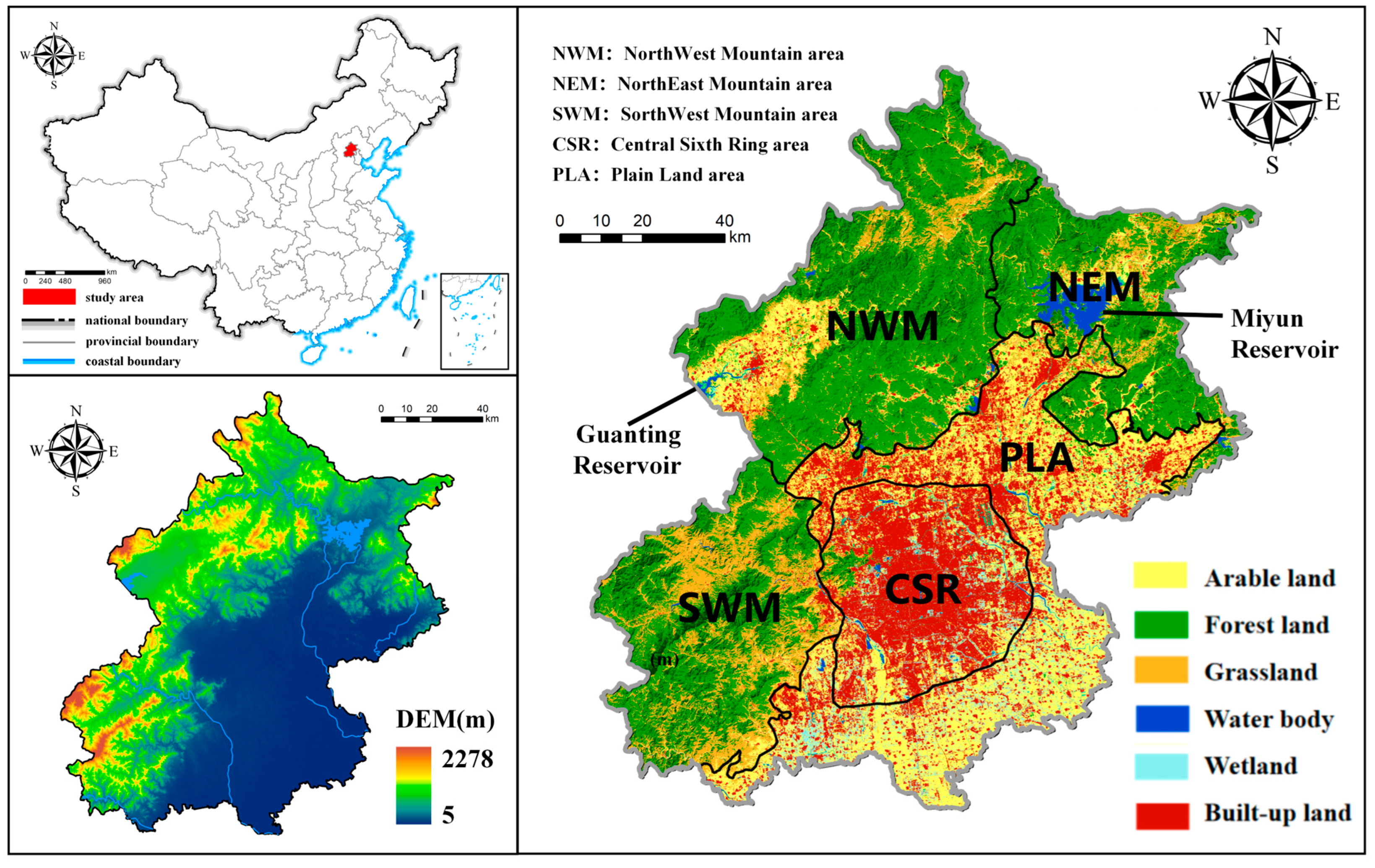
2.1. Study Area

Beijing (39°28′~41°05′ N, 115°25′~117°35′ E) lies on the northern edge of the North China Plain, at the southern base of the Yanshan Mountain Range. It is a world-renowned ancient capital and a contemporary worldwide metropolis. The northwest region of Beijing is dominated by the Yanshan tectonic belt and the folded mountain system of the northern part of the Taihang Mountains, forming high in the northwest and low in the southeast. The region experiences a warm temperate, semi-humid monsoon climate. The region experiences a warm temperate, semi-humid monsoon climate. In contrast to cities in southern China that receive over 1000 mm of annual rainfall, Beijing’s average yearly precipitation (500–600 mm) is relatively low, with approximately 75% falling between June and August in Beijing. The yearly average temperature is 11.7 °C. Summer temperatures are notably high, and the urban heat island effect is apparent [36]. In winter, the average temperature in urban areas is approximately 6 °C higher than in the surrounding mountainous regions. Precipitation during this season is limited. Beijing covers a total area of 16,410.5 km2. Beijing’s built-up area growth of approximately 1000 km2 since 2000 is notably higher than the average urban growth rate in China during the same period. The city’s population is 21.858 million, with approximately 50% residing in central urban districts, whose density and degree of urban agglomeration are significantly higher than the national urban average. However, the core urban population has declined by 19% in recent years, while the suburban population has increased significantly by 20.28%.
The Beijing City Master Plan (2004–2020) classifies urban zones according to the city’s natural background and specific functional attributes, including NWM, NEM, SWM, PLA, and CSR (Figure 1). The NWM, NEM, and SWM compose ecological screen areas within the city. The NWM encompasses the largest forested area, with a built environment adjacent to Guanting Reservoir in the west. The Miyun Reservoir in the NEM spans 180 km2 and is a key strategic water source for Beijing. The SWM features predominantly low to medium mountainous and hilly terrains, forming a crucial segment of the northern Taihang Mountains, characterized by warm-temperate zone deciduous broadleaf forest ecosystems. The PLA is a transitional plain between peripheral mountains and urban centers, with a few built-up areas distributed according to traffic lines. Urbanization has experienced significant growth over the past two decades. The CSR has the highest population density in Beijing. It exhibits a concentric pattern of urban expansion. The historical urban center, located within the Second Ring Road, serves as the core. Population density gradually decreases from the center toward the urban periphery.

2.2. Data Source

This study utilized multi-source meteorological, terrain, vegetation, and other datasets. The construction of the IRSEI model utilizes images from the Moderate-resolution Imaging Spectroradiometer (MODIS), developed by the United States National Aeronautics and Space Administration, using data from December–February and June–August as the raw data for winter and summer indicators. The EVI was obtained based on MOD13Q1, LST was obtained by processing MOD11A2, and WET, NDBSI, and DI were calculated using MOD09A1. The resolution was standardized to 250 m in ArcGIS after projecting and masking all indicator data to the extent of the study area. A more detailed description of the above data can be found in Table 1.
Based on existing research and data availability, we selected three major dimensions for analyzing the driving mechanisms of the IRSEI: natural, economic, and social factors. Population density (PD) represents a social factor and reflects the level of urbanization [37]. Nighttime Light (NTL) data were used as an economic indicator to assess consumption capacity and economic vitality [38]. Natural elements comprised evapotranspiration (ET), precipitation (Pre) [39,40], elevation (DEM), surface roughness (SR), minimum temperature (TEM), and wind speed (WS). SR was determined using slope values computed from DEM data. The following equation was used to calculate SR:
S R = 1 c o s ( S l p × π / 180 )
To address differences in dataset resolution, we pre-processed the data. In ArcGIS (version 10.8), we converted raster layers to point features and applied ordinary kriging to resample all variables to a consistent resolution of 250 m.
Table 1. Details of research data.
IndicatorSpatial ResolutionTemporal ResolutionSource
Enhanced vegetation index (EVI)250 m16 dayNASA a (MOD13Q1)
Land surface temperature (LST)1000 m8 dayNASA a (MOD11A2)
Wetness (WET)1000 m8 dayNASA a (MOD09A1)
Normalized difference build-up and soil index (NDBSI)1000 m8 dayNASA a (MOD09A1)
Difference index (DI)1000 m8 dayNASA a (MOD09A1)
Evapotranspiration (ET)500 myearlyNASA a (MOD16A2GF)
Nighttime Light (NTL)500 myearlyHDV b
Population Density (PD)100 myearlyWorldPop
Precipitation (Pre)1000 mmonthlyTPDC c
Minimum Temperature (TEM)1000 mmonthlyTPDC c
Wind Speed (WS)-dailyNOAA d
Elevation (DEM)30 m-NASA a
Surface Roughness (SR)30 m-NASA a
a National Aeronautics and Space Administration [41]; b Harvard Dataverse Repository; c National Tibetan Plateau Scientific Data Center; d National Oceanic and Atmospheric Administration [42].

2.3. Methods

2.3.1. IRSEI Model

The IRSEI selects five eco-indicators, including greenness, heat, humidity, dryness, and purity, which can intuitively reflect the quality of the regional ecological environment [21]:
I R S E I = f ( E V I , W e t , L S T , N D B S I , D I )
where EVI represents greenness index; Wet represents humidity index; LST represents heat index; NDBSI represents dryness index; and DI represents purity index. The following equations for each indicator are listed:
E V I = 2.5 × ( ρ n i r ρ r e d ) ( ρ n i r + 6 × ρ r e d 7.5 × ρ b l u e + 1 )
L S T = 0.02 × D N 273.15
W E T = 0.1147 ρ r e d + 0.2489 ρ n i r + 0.2408 ρ b l u e + 0.3132 ρ g r e e n 0.3122 ρ s w i r 1 0.6416 ρ s w i r 2 0.5087 ρ s w i r 3
S I = ( ρ s w i r 2 + ρ r e d ) ( ρ n i r + ρ b l u e ) ( ρ s w i r 2 + ρ r e d ) + ( ρ n i r + ρ b l u e )
I B I = 2 × ρ s w i r 2 / ( ρ s w i r 2 + ρ n i r ) ρ n i r / ( ρ n i r + ρ r e d ) ρ g r e e n / ( ρ g r e e n + ρ s w i r 2 ) 2 × ρ s w i r 2 / ( ρ s w i r 2 + ρ n i r ) + ρ n i r / ( ρ n i r + ρ r e d ) + ρ g r e e n / ( ρ g r e e n + ρ s w i r 2 )
N D B S I = ( S I + I B I ) / 2
D I = ρ r e a ρ n i r
where DN represents the gray scale value of land surface temperature; SI represents the bare soil index; and IBI represents index-based built-up Index. ρ r e d represents red light band reflectance; ρ n i r represents near-infrared band spectral emissivity; ρ b l u e represents blue light band reflectance; ρ g r e e n represents green light band reflectance; ρ s w i r 1 epresents short-wave infrared band reflectance; ρ s w i r 2 represents mid-infrared band reflectance; ρ s w i r 3 represents long-wave infrared band reflectance.
To ensure dimensional consistency among variables, we normalized each individual indicator. Considering the presence of large water bodies in the study area, such as the Miyun Reservoir, which could affect the humidity indicator and reduce the accuracy of EEQ assessment, we masked water bodies before further analysis. We then applied principal component analysis (PCA) to integrate the selected indicators and calculated the final IRSEI values, ranging from 0 to 1. Referring to the correspondence between the IRSEI range and the EEQ condition in Xu [17], we divided the IRSEI into five levels at 0.2 intervals, representing the worst, poor, moderate, good, and excellent levels.

2.3.2. Local Moran’s I

Local Moran’s I (LISA) is a widely used statistical method for identifying patterns of local spatial clustering [43]. Moran’s I can be divided into the Global Moran’s I and the Anselin Local Moran’s I. The Global Moran’s I assess the overall spatial autocorrelation across the study area. In contrast, the Local Moran’s I captures the degree of spatial association around individual locations. In this study, we applied the Local Moran’s I to quantify spatial autocorrelation at each sampling point. Based on the results, spatial units can be categorized into four types of spatial association: high-high (H-H), low-low (L-L), high-low (H-L), and low-high (L-H). These categories reflect the relationship between the attribute values of a given location and those of its neighboring areas. The calculation formula is as follows:
I i = ( x i x ¯ ) S 2 · j = 1 n ω i j ( x i x ¯ )
where I i is the local Moran index of the ith spatial cell; x i is the observed value of cell i; x ¯ is the mean value of all cells; S 2 is the variance of the observations; ω i j and is the normalized spatial weight matrix element.

2.3.3. Redundancy Analysis

Redundancy Analysis (RDA) is a multivariate statistical technique used to model linear relationships between the response variable matrix and the explanatory variable matrix [44]. It combines regression and principal component analysis to assess how much variation in the response data can be explained by the explanatory variables. RDA facilitates the assessment of explanatory power and statistical significance of individual environmental factors. In this study, we used Canoco 5.0 to visualize the relationships among ranked objects, explanatory variables, and response variables by ordination diagrams. The results can display the interpretation rate and significance test results of each environmental factor. The cosine of the angle between the vectors of a response variable and an explanatory variable indicates the strength and direction of their correlation, which also applies to the angles between pairs of explanatory variables. However, the angle between response variables does not convey meaningful information about their correlation. As shown in Figure 2, angle ∠a is close to 90°, indicating no correlation between Rv1 and Ev3, and angle ∠b falls between 0° and 90°, suggesting a positive correlation between Rv2 and Ev1. Finally, angle ∠c lies between 90° and 180°, which suggests a negative correlation between Rv1 and Ev2.

3. Results

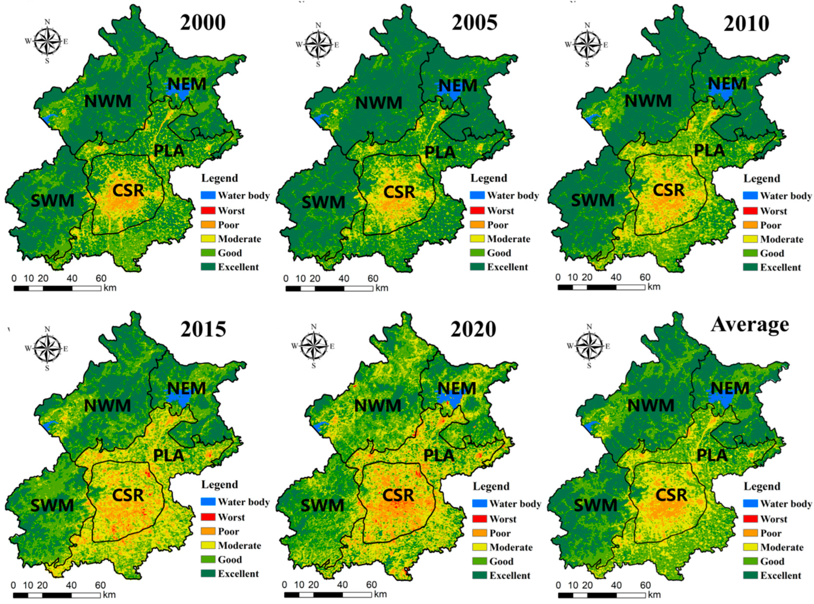
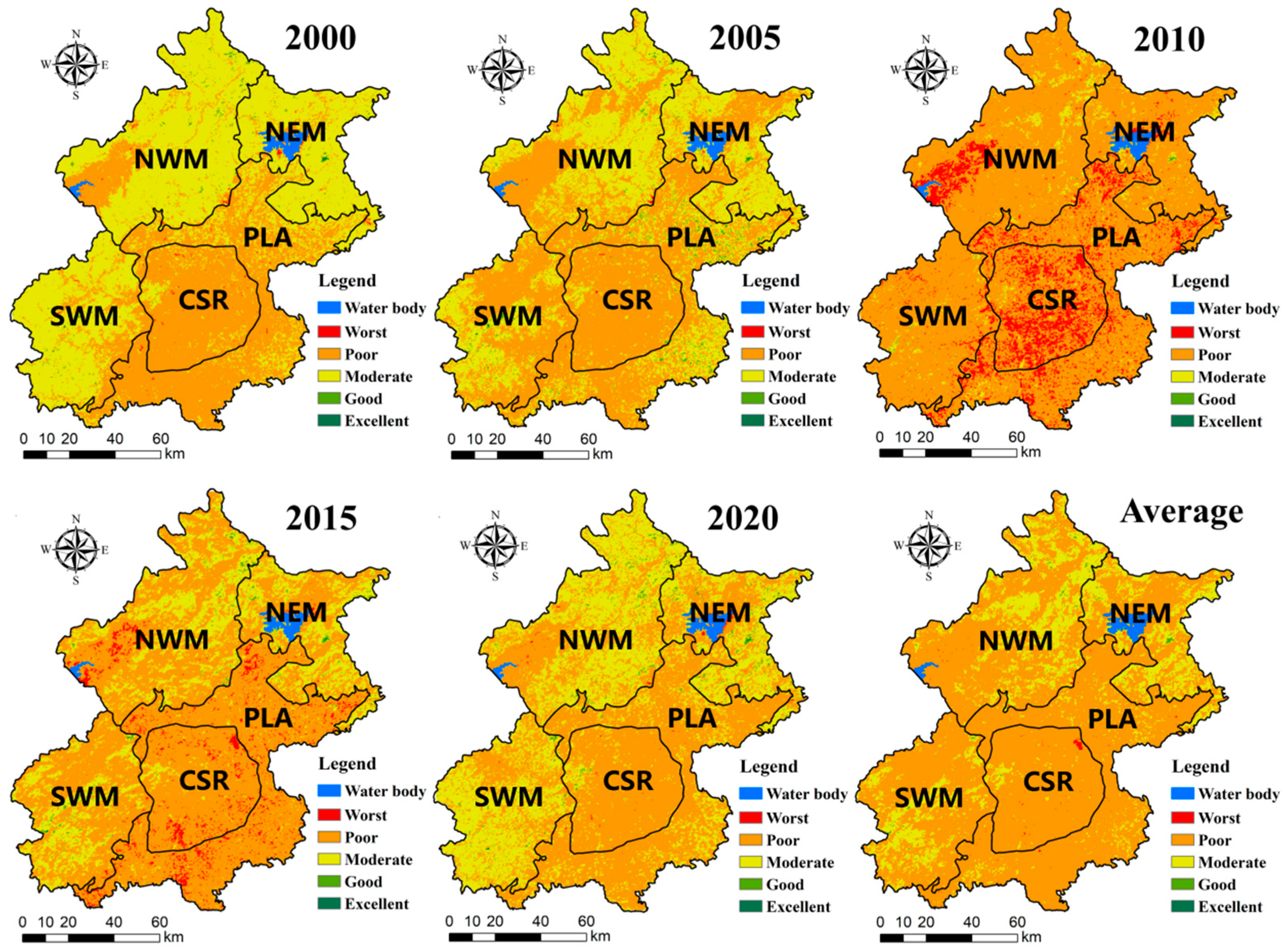
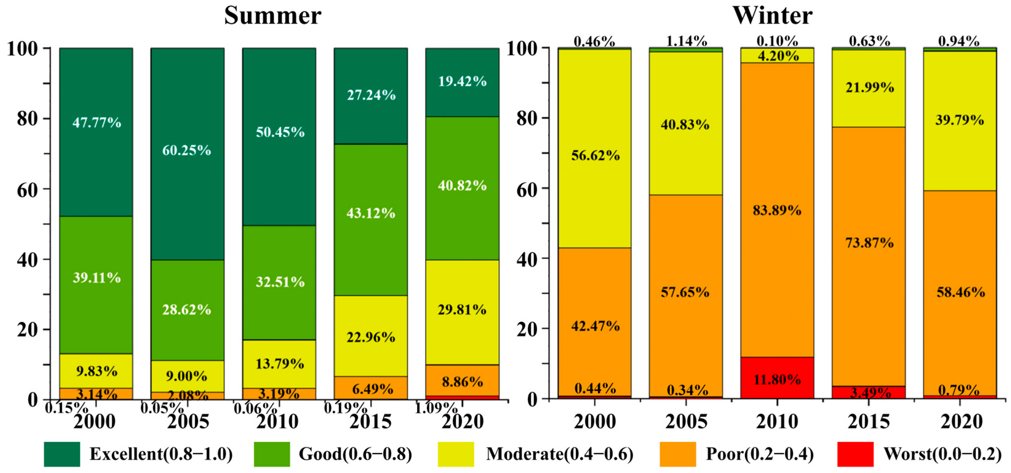
3.1. Spatial Pattern and Dynamics of IRSEI

The average IRSEI of Beijing was higher in summer (0.69) than in winter (0.34) during 2000 to 2020. The standard deviation of IRSEI values across districts also showed seasonal differences, with a higher value in summer (0.10) than in winter (0.04). Variations in EEQ among subdistricts were more pronounced in summer. The spatial distribution of IRSEI followed the pattern in summer: NWM (0.76) > SWM (0.75) > NEM (0.74) > PLA (0.64) > CSR (0.52) (Figure 3). This trend reflects a general spatial decline in EEQ, from mountainous regions to plains and finally to urban centers. The winter pattern was slightly different but still showed mountainous areas with higher values: NWM (0.37) > NEM (0.36) > SWM (0.35) > PLA (0.30) > CSR (0.27) (Figure 4). Mountain areas remained the primary zones of high EEQ. However, the EEQ in the PLA and CSR regions tended to converge during winter.
The summer IRSEI in Beijing (Table S1) demonstrated an upward trajectory from 2000 to 2010, followed by a decline through 2020. The highest value was recorded in 2010 (0.76), while the lowest appeared in 2020 (0.52). Across the entire region, the proportion of areas with excellent EEQ ranged from 19.42% to 60.25% (Figure 5). The NWM, NEM, and SWM consistently showed high EEQ between 2000 and 2010. Approximately 65% of these mountainous regions achieved excellent levels of EEQ, and 33% reached good in 2000. The proportion of areas with excellent EEQ increased by approximately 15% by 2005 and remained stable through 2010. The PLA, a transitional zone between mountains and urban development, reached its highest EEQ performance in 2005. 89% of the PLA achieved good or excellent EEQ ratings in the same year. However, this proportion declined steadily—from 50.5% to 33.2% from 2005 to 2020. The proportion of NWM, NEM, and SWM areas with excellent EEQ decreased significantly from 2010 to 2020. Compared to 2010, the share dropped by 30% in 2015 and continued to decline by another 17% by 2020. The NEM experienced the most severe decline. High-level EEQ zones in the NWM became increasingly fragmented, and isolated low-EEQ zones emerged in both the CSR and PLA regions for the first time.
The winter IRSEI (Table S2) showed a declining trend from 2000, reaching its lowest point in 2010 with a value of 0.29. The IRSEI in 2000 was higher than that in 2020, reaching 0.42—the highest winter value during the study period. Areas with poor EEQ accounted for 42.47% to 83.89% of the total region during the study period. The northern and southern parts of the NWM, the northeastern NEM, and the central SWM observed a notable decrease in EEQ. These areas experienced a shift from moderate to poor EEQ levels by 2005, resulting in a 15.79% reduction in the areas with moderate EEQ across the study region. In 2010, regions with poor and worst EEQ levels accounted for 83.89% and 11.80% of the total area, respectively. Severe ecological degradation occurred in certain regions, including the built-up zone surrounding the Guanting Reservoir in the southwestern part of the NWM, the northern portion of the PLA, and both the peripheral and central areas of the CSR. Most other areas had also declined to the poor EEQ level. By 2015, signs of ecological recovery emerged. The proportion of the city reaching a moderate EEQ level increased by 17.79%, primarily in the NWM, NEM, and SWM. However, this improvement was spatially fragmented. Regions with the worst EEQ levels had largely disappeared by 2020. Most areas across the city, except for southwestern NWM, northern NEM, and northern SWM, had reached a moderate EEQ level. However, the PLA and CSR remained predominantly at the poor level.

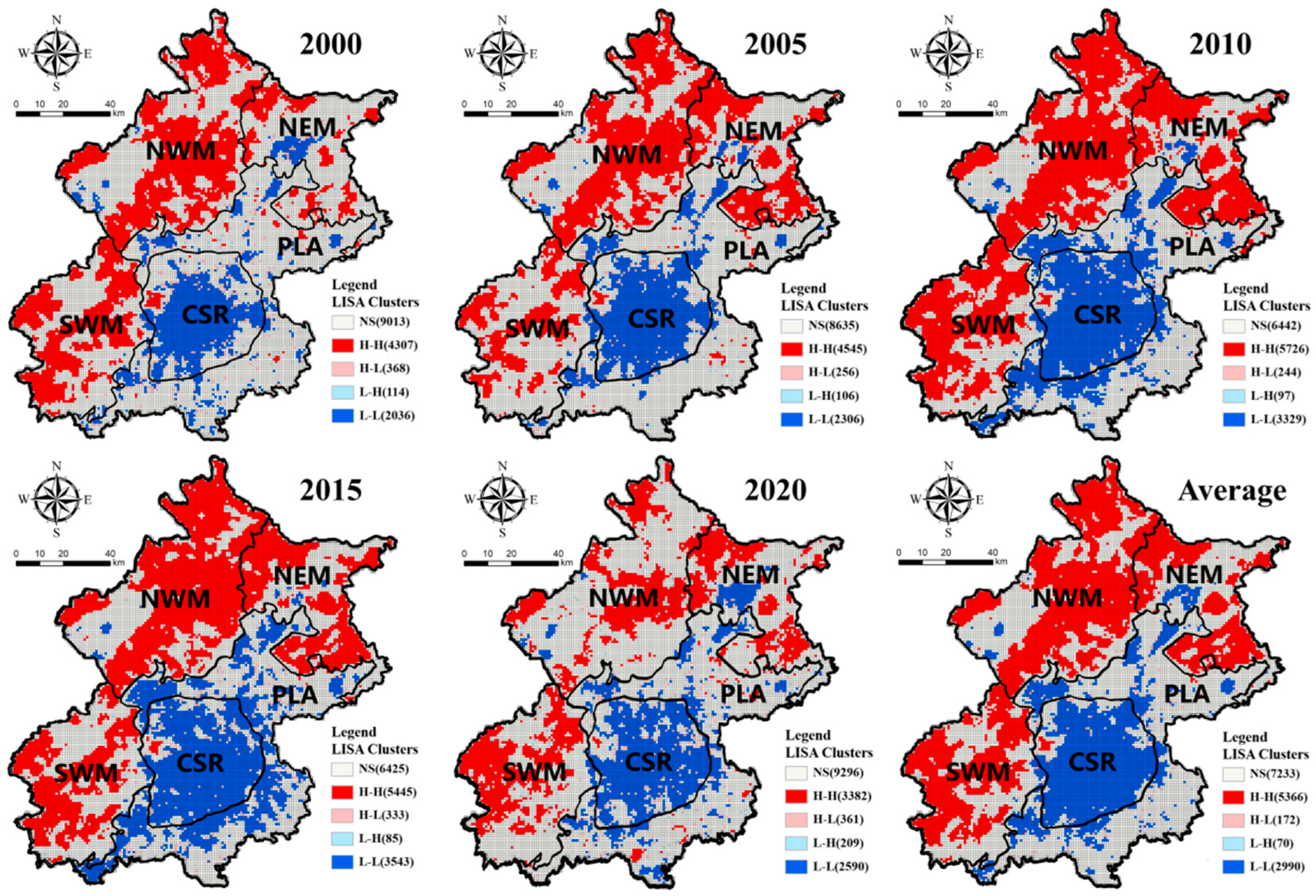
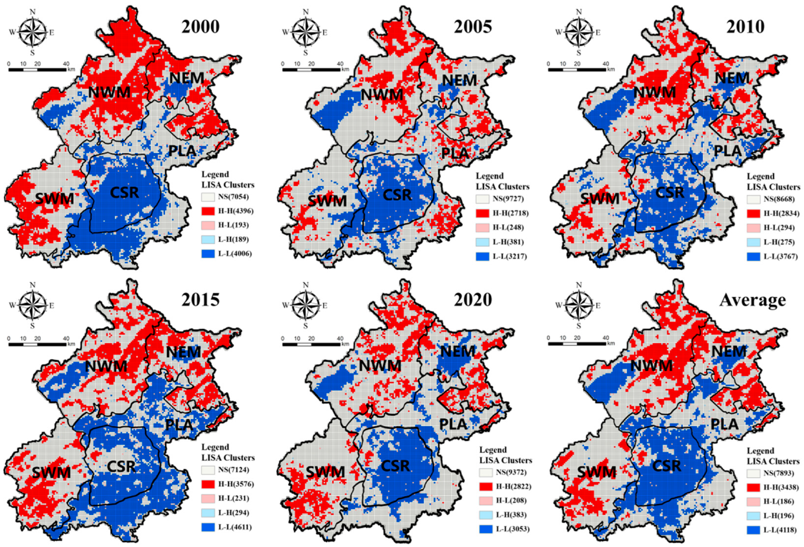
3.2. LISA Cluster Character of IRSEI

The LISA analysis shows that L-L clusters primarily concentrate in the central area of the CSR. In contrast, H-H clusters dominate the NWM, NEM, and SWM regions. PLA, as a transition zone, its northern part and the adjoining zone of CSR become the area of L-L clusters. Aside from the winter of 2015, its L-L clusters mainly emerged in the CSR and the outer northern, eastern, and western parts of the PLA. Overall, the EEQ spatial autocorrelation results are consistent with the IRSEI analysis.
The H-H clusters of EEQ continued to expand from 2000 to 2010 and decreased significantly between 2010 and 2020 in the summer (Figure 6). The quantity of L-L clusters showed a consistent upward trend, peaking at 3543 in 2015. The H-H clusters in EEQ in 2010 were the most with the value of 5726, while the H-H clusters of EEQ reduced to 3328 in 2020. In addition to the northwestern area being the main distribution area of H-H clusters, a small number of H-H clusters also occur in the western CSR. A comparison between 2000 and 2005 shows a 22.4% increase in EEQ H-H clusters in NEM and a 13.6% increase in low-value clusters in CSR, accompanied by a spatial expansion from the center to the periphery. In 2010, H-H clusters became more concentrated, with the high-value and low-value zones collectively accounting for 57% of the total domain area. Among them, H-H clusters in NWM, SWM, and NEM increased to 63.0%, 52.0%, and 53.4%, respectively, and CSR L-L clusters covered more than 81.4% of the area. In 2015, L-L clusters expanded further to the northeast in PLA, and their percentage decreased by 3.8%. An accelerated decline occurred in both H-H and L-L clusters in 2020. In detail, H-H clusters in NWM, NEM, and SWM declined by 34.6%, 19.3%, and 4.7%, while L-L clusters in PLA and CSR decreased by 18.7% and 11.3% (Figure S1).
The overall EEQ demonstrated a fluctuating trend of H-H and L-L clusters decreasing in winter (Figure 7). The degree of EEQ clustering ranked in descending order as follows: NWM > NEM > SWM > PLA > CSR. In 2000, L-L clusters were predominantly located in the southwestern region of PLA and CSR, comprising 79.8% and 35.6%, respectively. H-H clusters primarily appeared in the northeastern part of NWM, the western part of SWM, and the southeastern and northwestern regions of NEM. The number of H-H clusters declined sharply in 2005, with a 24.7% decrease in NWM, a 5.8% increase in NEM, and a 21.3% decrease in SWM. A few H-H clusters also remained in eastern PLA. L-L clusters in the CSR displayed a fragmented pattern, with their total area shrinking to 63.8% in 2010. Relative to 2005, H-H clusters declined significantly in the PLA, whereas L-L clusters increased by 13.6%. The central region of CSR has long served as a major hotspot for L-L clusters in EEQ. However, spatial autocorrelation weakened in the winter of 2015, and L-L clusters shifted toward the PLA and northern, eastern, and southern outskirts of CSR. By 2020, H-H clusters had declined by 5%, with the most significant reductions observed in central NWM. L-L clusters decreased by 10%, mainly concentrated in the junction area between PLA and CSR.

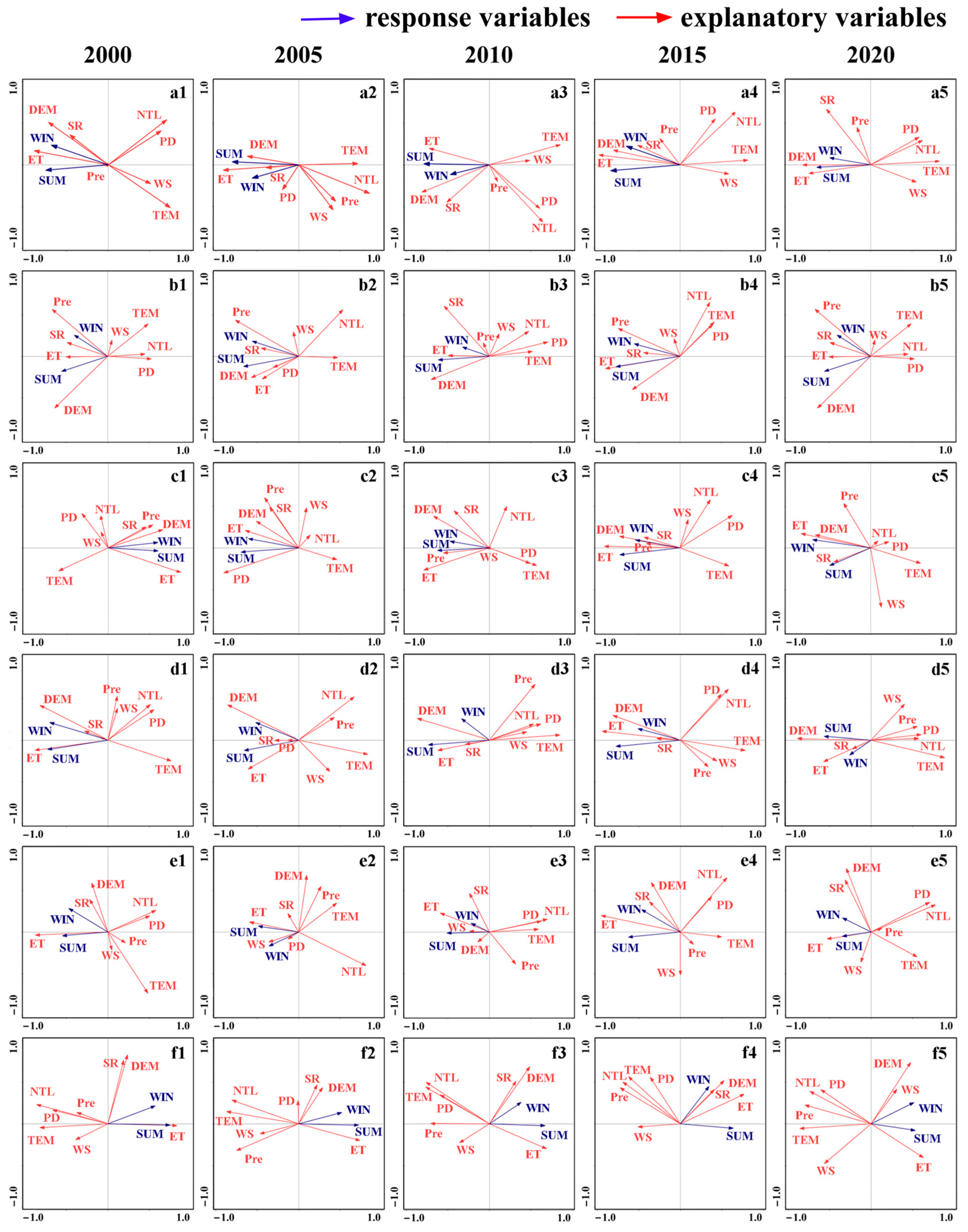
3.3. Natural-Economic-Social Factors of IRSEI

The results of the driving factor analysis from 2000 to 2020 (Figure 8) show that ET and DEM were the primary positive contributors to EEQ, with contribution rates ranging from 17.4% to 82.2%. TEM functioned as a negative influence, with an explanatory power of 40.9% in 2010. These findings highlight the dominant role of natural factors in shaping EEQ. PD showed a negative correlation with EEQ in all years except 2005. However, its contribution remained low, between 0.5% and 3.1%, suggesting that social factors exerted a weak and indeterminacy influence on urban EEQ in Beijing. NTL, which reflects regional economic activity, contributed between 3.3% and 17.2% to EEQ throughout the study period. This result underscores the higher impact of economic considerations over social ones on EEQ. Seasonal differences were also evident. ET and NTL exerted more pronounced effects on EEQ in summer, but DEM and SR had a more significant impact during winter. The influence of other factors alternated between seasons, indicating a dynamic interaction between factors and seasonal environmental conditions.
The analysis of zonal driving factors revealed that ET, DEM, and SR were the primary positive drivers of EEQ. Among them, ET was the most influential, dominating multiple periods. Its contribution peaked in several years, with a maximum of 86.6%. Overall, ET affected summer EEQ more than winter. DEM consistently showed a stable positive correlation with winter EEQ and exhibited a stepwise increasing trend over time. In the NEM, DEM’s contribution rose from 13.3% in 2005 to 25.0% in 2010 and 30.5% in 2020. Its explanatory power demonstrated a stepwise increase. DEM showed limited influence on EEQ in PLA and CSR, with contribution rates below 10%. It also revealed a strong correlation with SR. SR consistently acted as a positive driver across the entire time series in NWM and SWM. However, its association with IRSEI noticeably weakened during the winter of 2005 and the summer of 2020.
The negative drivers of EEQ were TEM, NTL, and PD. TEM emerged as a significant adverse driver across the study area, exerting strong suppressive effects in NEM, SWM, and PLA, with a maximum contribution of 74.7% in SWM. The intensity of inhibition of TEM on EEQ changes was generally higher in summer than in winter, but the dominant effect was higher in NEM in winter. The NTL and PD formed a significant synergistic negative correlation on EEQ. In 2000, NTL emerged as the primary driver of EEQ in the CSR. It explained 40.2% of the EEQ variation and contributed 73.1%, surpassing the influence of TEM. PD had a positive effect on EEQ in 2005. In the same year, NTL contributed 23.9% to EEQ, making it the second most influential explanatory factor in the NWM. PD became the dominant driver of EEQ in the NWM region in 2010. Its explanatory power increased to 13.1%, and its contribution to EEQ rose to 49%. In 2000 and 2020, the directions of NTL, PD, and TEM vectors of CSR strongly coincide, thus demonstrating a high degree of correlation and significant spatial coupling. These factors exerted a marked suppressive effect on summer EEQ together.
The influence of Pre and WS on EEQ varied across zonal and temporal dimensions. The effect of WS exhibited pronounced spatiotemporal heterogeneity. WS exhibited a suppressive effect on EEQ in the SWM while serving as a significant promotive factor in PLA. The relationship between WS and EEQ in CSR shifted over time, exhibiting a negative influence in the early years and a positive influence in both summer and winter in later years. Pre generally served as a positive driver of EEQ in NWM and NEM, while it showed a negative correlation with EEQ in SWM, PLA, and CSR. Pre explained 42.6% of the NEW EEQ spatial variation in 2020 and emerged as a secondary suppressor in SWM. Pre had a higher intensity of summer EEQ than winter in CSR throughout the study period.

4. Discussion

4.1. Analysis of the Spatiotemporal Pattern and Dynamics of EEQ

Beijing’s EEQ gradually declined from mountainous and plain regions toward urban areas. This spatial pattern aligns with the findings of Zhu et al. [45], who reported similar trends in the ecological environment along the Middle Route of the South-to-North Water Diversion Project (MR-SNWDP) in China. Mountainous regions host diverse natural resources, including forests, water bodies, and wetlands. Vegetation in these areas helps lower atmospheric temperatures through latent heat flux and retains dust via leaf surface adsorption, trunk interception, and wax accumulation [46]. Moreover, diverse habitats in mountainous areas support various species of birds, insects, and small mammals, contributing to better ecosystem stability [47]. Due to their high specific heat capacity compared to other land surfaces, wetlands and watersheds play a critical role in regulating local microclimates and improving air quality. Impervious surfaces and densely packed buildings concentrate in cities. These features suppress latent heat exchange and reduce the natural purification functions of vegetation, water, and the atmosphere. Consequently, they contribute to ecological problems such as air pollution and water quality degradation. Urbanization also intensifies the greenhouse and heat island effects, leading to higher ambient temperatures. This further disrupts ecosystem self-regulation mechanisms, such as pollutant dispersion and water cycling, thereby accelerating the degradation of EEQ in urban environments [48]. Summer EEQ in the urban core continued to decline during the study period, accompanied by an expansion of L-L clusters. The decline in wetland areas, increased fragmentation of green space, and expanding coverage of urban buildings and transportation infrastructure were the primary drivers of this change in Beijing’s CSR region [49].
Air quality played a role in shaping winter EEQ patterns, particularly in haze-prone areas such as the CSR and PLA regions. Compared to RSEI, the IRSEI model incorporating the DI produced relatively lower values in winter, reflecting the influence of atmospheric conditions like haze and reduced visibility [50]. From 2001 to 2020, PM2.5 exposure risk in Beijing showed a downward trend, as the city implemented a series of policies to mitigate air pollution and improve environmental quality [51]. The inclusion of DI helps adjust for these region-specific atmospheric effects, enhancing the accuracy of EEQ assessment under conditions commonly experienced in northern megacities such as Beijing. Beijing’s EEQ showed a steady improvement in summer from 2000 to 2010. The improvement in the western region was probably affected by the Beijing–Tianjin Sandstorm Source Control Project (BTSSCP), implemented by the Chinese government. During the implementation of this project, Beijing established approximately 73,300 hectares of windbreak and sand-fixation forests. Hebei Province implemented effective management measures in windblown sand hazard zones, particularly to the west and north of the city [52]. At the end of the project in 2010, the overall ecological risk level in Beijing was lower than that in 2000, with most areas in the Medium-Low class [53]. Windbreak and sand-fixation forests effectively mitigated dust pollution caused by construction activities and exposed soil, particularly under windy and arid conditions in and around Beijing.
During the study period, EEQ in mountainous areas during winter showed a mixed distribution of poor and moderate levels. In contrast, PLA and CSR exhibited a more homogeneous pattern dominated by lower EEQ values. Vegetation plays a critical role in regulating near-surface temperature and humidity, as well as retaining dust, all of which are vital for maintaining EEQ. Vegetation across Beijing, including mountain forests, plain croplands, and urban green spaces, enters the withering period in winter. As a result, surface landscapes across these zones become more uniform, leading to a more evenly distributed EEQ pattern. Moreover, greenness represents the first principal component of the IRSEI, and Beijing’s vegetation is primarily composed of closed deciduous broadleaf forests. These forests emit biogenic volatile organic compounds (BVOCs), mainly isoprene and monoterpenes, which make up more than 50% of the total BVOC emissions. These chemicals reduce near-surface stresses, including elevated temperatures, radiation, and oxidative pressure [54]. However, the withering of deciduous forests leads to reduced BVOC emissions and a diminished capacity to regulate ecological conditions during winter. This seasonal decline explains the lower IRSEI values in winter compared to summer and the more uniform spatial distribution on EEQ.
Winter EEQ reached its lowest level in 2010, with the highest concentration of severe degradation observed in the PLA and CSR. As urbanization has intensified ecological damage, the Chinese government has specifically established national binding targets for energy conservation and emission reduction during the implementation of the outline of its 12th Five-Year Plan for economic and social development from 2011 to 2015. Throughout the execution of the plan, national NOx emissions declined by over 10% and continued to decrease in subsequent years, leading to an overall improvement in EEQ [55]. Since 2010, Beijing has successively introduced the Beijing Clean Air Action Plan, the Beijing Clean Air Action Plan 2013–2017, and other eco-environmental treatment policies. In 2013, Beijing also launched the “coal-to-electricity” heating method to reduce CO2, SO2, NOx, and other pollutants [56], and the overall NO2 in Beijing showed a significant decrease, with the largest decrease in the high-emission city center [57]. Beijing experienced its lowest winter EEQ in 2010, with the most pronounced decline occurring in CSR and the PLA, where degraded ecological conditions covered the widest.

4.2. Driving Mechanism of EEQ

IRSEI changes are a complex process driven by the combination of natural, economic, and social factors. In this study, the selected driving variables explained 36.5–56.7% of the variation in IRSEI across Beijing. As a core component of the hydrological cycle and energy balance, ET substantially influences regulating surface temperature, mitigating the urban heat island effect, and improving the regional microclimate. However, when actual ET exceeds the ecosystem’s water balance threshold, it may trigger surface drying, resulting in increased soil exposure and reduced vegetation cover [58]. Such conditions can degrade EEQ, potentially explaining the observed summer increase in L-L clusters and the decline in H-H clusters during winter. Pre affects EEQ unevenly across regions and shows limited explanatory strength at the municipal scale in Beijing. Two main factors may account for this pattern. On the one hand, Pre is inherently stochastic, and significant differences exist in its interannual and seasonal variability. The variabilities in intensity, frequency, and type make it difficult to establish a stable correlation between annual precipitation and EEQ [59]. On the other hand, Beijing lies in a semi-humid climatic zone, where water is not the primary limiting factor for vegetation growth. As a result, the indirect effect of precipitation on EEQ remains relatively weak.
Although WS generally acts as a suppressor of EEQ at the citywide scale, its influence varies significantly across spatial zones. Wind enhances thermal coupling at the surface-atmosphere interface, increases evapotranspiration [60], and reduces the leaf surface temperature gradient. These processes help mitigate the physiological stress on plant photosynthetic organs caused by solar radiation and heat [61]. This mechanism is particularly evident in the PLA, and its open terrain enables wind to exert a positive effect by facilitating the dispersion of air pollutants. However, strong winds can intensify wind erosion and enhance the dispersion of particulate matter such as dust and pollen. This increases atmospheric turbidity, especially in CSR, where pollutant emissions from industry and traffic are high and wind-pollinated plants are common. These findings highlight the dual nature of WS effects on EEQ, which differ by spatial scale and regional context. Surface morphology indirectly affects spatial and temporal EEQ patterns through its influence on runoff, local climate, and vegetation distribution [62]. NWM, NEM, and SWM exhibit consistently higher levels of EEQ due to their complex geomorphology and dense vegetation. Pre regulates soil moisture availability, facilitates nutrient cycling, and enhances plant water-use efficiency, thereby promoting aboveground biomass accumulation and improving overall ecosystem productivity [63]. Pre acts as a positive driver of EEQ in NWM and NEM. However, Pre shows a negative relationship with EEQ in SWM, PLA, and CSR. These contrasting effects emphasize the role of topography in indirectly influencing EEQ through precipitation patterns.
In addition to natural factors, economic considerations also influence EEQ. Both PD and NTL have indirect adverse effects on EEQ [64]. In Beijing, human activities are primarily concentrated in lowland areas with gentle terrain, while mountainous regions tend to have lower population densities. As a result, the negative influence of PD and NTL on EEQ is weaker in NWM, NEW, and SWM, corresponding to the widespread distribution of H-H clusters. The urbanization process characterized by PD is closely related to the ecological carrying capacity and shows a negative dynamic relationship with EEQ [65]. However, based on the construction of a cross-regional ecological compensation mechanism and the optimization of spatial structure, the transformation of urbanization and EEQ from uncoordinated to coordinated can be gradually realized [66], which can explain the positive correlation between PD and EEQ of NWM and NEM in 2005. NTL, a key social factor, can disrupt biological rhythms and alter ecological community structures, ultimately reducing EEQ [67]. Prior studies have demonstrated an inverted U-shaped relationship between EEQ and economic development [68]. NTL accounts for up to 40.2% of the variance in EEQ of the highly populated CSR. This strong association suggests a pronounced negative impact, which may help explain why EEQ levels in CSR consistently remain the lowest across Beijing.

4.3. Complexity of EEQ

The drivers selected in this study were able to explain up to 45.75%, 44.91%, 53.54%, 37.07%, and 54.96% of the IRSEI results for NWM, NEM, SWM, PLA, and CSR, indicating that additional factors may be influencing the changes in spatial-temporal dynamics patterns of IRSEI. Beyond the quantitative drivers analyzed in this study, government policies related to infrastructure development and ecological restoration have influenced land cover change, indirectly shaping EEQ dynamics. Beijing’s urbanization rate increased rapidly from 26.4% to 62.7% from 1990 to 2019 [69]. Construction land in Beijing increased by 988.99 km2 (Figure S2), primarily encroaching on former cropland and grassland. Beijing experienced a continuous decline in arable land, with a net loss of 489.09 km2 from 2000 to 2020. The forest land showed an overall trend of increase followed by a decrease, peaking at 6470.19 km2 in 2015. The expansion of construction land, together with the loss of arable land and forest land, contributed to the observed decline in EEQ [70], particularly aligning with the downward trend during the summers of 2015 to 2020. Land cover changes driven by a complex interplay of natural, economic, and social factors can be quantitatively analyzed using land use transfer matrices. However, the specific effects of ecological restoration and similar policies on EEQ are challenging to quantify and require further methodological development.
This study did not assess the impact of transportation-related factors on EEQ in Beijing, despite a significant increase in motor vehicle ownership from 1.578 million in 2000 to 6.57 million in 2020 [71]. In winter, atmospheric stability impedes the diffusion of vehicular PM2.5 emissions, while NOx released from traffic contributes to haze formation. These conditions may be associated with the observed decline in winter EEQ from 2000 to 2020, particularly in the central area of the CSR. In recent years, increased summer rainfall has raised the risk of urban flooding [72], particularly in SWM [73]. Heavy rainfall generates high runoff volumes, which can damage transportation infrastructure in densely populated areas and pose risks to public safety. Notably, EEQ in SWM during the summer months is lower than, or comparable to, that in NWM and NEM, with lower EEQ zones concentrated near valley lines. Furthermore, runoff-induced pollution can create secondary environmental hazards that exacerbate EEQ degradation [74]. However, such heavy rainfall events are episodic and do not exert a consistent or long-term influence on EEQ patterns. Similarly, the lockdowns imposed due to the pandemic since 2019 have led to short-term improvements in air quality, with significant reductions in PM2.5 concentrations, thereby indirectly enhancing urban ecological environmental quality during the periods of restriction [51]. While both events can temporarily alter environmental conditions, their irregular occurrence and transient effects limit their explanatory power in identifying the long-term drivers of EEQ dynamics. Therefore, future research should incorporate transportation and hydrological factors with greater temporal depth, while also distinguishing between structural and episodic influences on urban ecological quality.

5. Conclusions

In this study, we focused on Beijing as the study area and calculated the IRSEI for both winter and summer from 2000 to 2020. We examined the spatiotemporal evolution of EEQ across different territorial and spatial zones. Based on this analysis, we investigated the driving mechanisms of EEQ and assessed their complexity. The main conclusions are summarized as follows:
The IRSEI in Beijing demonstrates pronounced spatiotemporal heterogeneity, with EEQ exhibiting distinct spatial patterns across seasons. In summer, IRSEI generally declines from the surrounding mountainous areas toward the urban core. The mountainous regions—NWM, NEM, and SWM—consistently exhibit high EEQ, while PLA is the transitional buffer zone. The CSR persistently shows the lowest EEQ values. Winter EEQ shows a similar spatial pattern, but overall EEQ levels are markedly lower than in summer. Throughout the study period, summer EEQ followed a rise-then-decline trajectory, peaking in 2010 and dropping to its lowest level by 2020. The proportion of high-EEQ areas in NWM, NEM, and SWM gradually decreased. Winter EEQ declined to its lowest point in 2010, followed by a gradual recovery, particularly in CSR. L-L clusters were mainly concentrated in central CSR, while H-H clusters were distributed across NWM, NEM, and SWM. Northern PLA and its adjacent areas near CSR exhibited widespread L-L clustering. Except for winter 2015, when L-L clusters became more dispersed and concentrated in the northern, eastern, and western of CSR and PLA.
Natural factors predominantly influenced driving EEQ dynamics in Beijing during the study period. Annual evapotranspiration and elevation consistently emerged as the most influential positive drivers of EEQ change, while annual minimum temperature exhibited a strong negative effect. Evapotranspiration played a dominant role in shaping long-term EEQ trends across different regions. Both surface roughness and elevation were significantly and positively associated with EEQ. In contrast, annual minimum temperature had a pronounced negative effect on EEQ in NEM and SWM. Socioeconomic factors such as population density and nighttime light intensity exerted comparatively minor effects on EEQ. However, both variables showed strong positive correlations with EEQ in the CSR, particularly during the summer months. Interannual precipitation did not exhibit a consistent or significant relationship with EEQ across the study period. The influence of wind speed on EEQ varied across regions and lacked a clear directional trend, indicating uncertainty in its overall effect. Notably, the selected variables in this study could only account for 44.91% to 54.96% of the variation in IRSEI at the district level. This result suggests that additional factors—beyond those included in the current model—probably significantly influence the spatiotemporal dynamics of EEQ. Future studies should further explore these unquantified drivers.
This study focuses on the continuous natural, social, and economic factors that influence EEQ. The impacts of episodic events are discussed briefly without quantitative analysis. Although the IRSEI enhances the assessment of EEQ, further refinement is needed to better account for seasonal variations in specific regions. Future research should consider integrating multi-source data and incorporating measurable long-term socioeconomic policy effects to strengthen the robustness and applicability of EEQ evaluations.

Supplementary Materials

The following supporting information can be downloaded at: https://www.mdpi.com/article/10.3390/su17136056/s1, Figure S1. The ratio of IRSEI LISA Clusters. Figure S2. The transfer matrix of land use types. Table S1. the mean, median, and standard deviation of IRSEI in different functional zones in summer. Table S2. the mean, median, and standard deviation of IRSEI in different functional zones in winter

Author Contributions

Conceptualization, G.L.; formal analysis, J.W. (Jingyi Wang); investigation, J.W. (Jinghan Wang); data curation, J.W. (Jinghan Wang) and J.J.; writing—original draft preparation, J.W. (Jingyi Wang); writing—review and editing, J.W. (Jingyi Wang) and G.L.; visualization, J.W. (Jingyi Wang) and J.J. All authors have read and agreed to the published version of the manuscript.

Funding

This work was supported by the National Key Research and Development Program of China [Grant No. 2023YFC3804004] and the National Natural Science Foundation of China (42371274).

Institutional Review Board Statement

Not applicable.

Informed Consent Statement

Not applicable.

Data Availability Statement

The raw data supporting the conclusions of this article will be made available by the authors on request.

Acknowledgments

We would like to thank the editor and anonymous reviewers for reading the manuscript and providing valuable recommendation during their busy schedule. We also thank Shu Tao from the National Geomatics Center of China for her significant contributions to the study design and data support.

Conflicts of Interest

The authors declare that they have no known competing financial interests or personal relationships that could have influenced the work reported in this study.

Abbreviations

The following abbreviations are used in this manuscript:
CSRCentral Sixth Ring area
DEMElevation
EEQEcological Environment Quality
ETEvapotranspiration
LISALocal Moran’s I
InVESTIntegrated Valuation of Ecosystem Services and Tradeoffs
IRSEIImproved Remote Sensing Ecological Index
NTLNighttime Lighting Index
NEMNortheast Mountain area
NWMNorthwest Mountain area
PDPopulation density
PLAPlain Land area
PrePrecipitation
PSRPressure–State–Response
RDARedundancy Analysis
RSEIRemote Sensing Ecological Index
SRSurface Roughness
SWMSouthwest Mountain area
TEMMinimum Temperature
WSWind Speed

References

  1. Azurza-Zubizarreta, O.; Basurko-PerezdeArenaza, I.; Zelarain, E.; Villamor, E.; Akizu-Gardoki, O.; Villena-Camarero, U.; Campos-Celador, A.; Barcena-Hinojal, I. Urban Energy Transitions in Europe, towards Low-Socio-Environmental Impact Cities. Sustainability 2021, 13, 11641. [Google Scholar] [CrossRef]
  2. Fastenrath, S.; Braun, B. Lost in Transition? Directions for an Economic Geography of Urban Sustainability Transitions. Sustainability 2018, 10, 2434. [Google Scholar] [CrossRef]
  3. Kołsut, B.; Kudłak, R. From systemic to sustainability transitions: An emerging economy perspective on urban sprawl and the automobile revolution. Eur. Urban Reg. Stud. 2023, 31, 149–167. [Google Scholar] [CrossRef]
  4. United Nations. World Urbanization Prospects 2018: Highlights. United Nations, Department of Economic and Social Affairs, Population Division. 2018. Available online: https://population.un.org/wup/assets/WUP2018-Highlights.pdf (accessed on 20 September 2020).
  5. Laurance, W.F.; Engert, J. Sprawling cities are rapidly encroaching on Earth’s biodiversity. Proc. Natl. Acad. Sci. USA 2022, 119, e2202244119. [Google Scholar] [CrossRef]
  6. Marley, H.G.; Dirks, K.N.; Neverman, A.J.; McKendry, I.; Salmond, J.A. The Relationship Between Brown Haze, Atmospheric Boundary Layer Structure, and Air Pollution in an Urban Area of Complex Coastal Terrain. Atmosphere 2021, 12, 101057. [Google Scholar] [CrossRef]
  7. Middleton, N.; Kang, U. Sand and Dust Storms: Impact Mitigation. Sustainability 2017, 9, 1053. [Google Scholar] [CrossRef]
  8. Thackeray, C.W.; Hall, A.; Norris, J.; Chen, D. Constraining the increased frequency of global precipitation extremes under warming. Nat. Clim. Change 2022, 12, 441–448. [Google Scholar] [CrossRef]
  9. Tuel, A.; Steinfeld, D.; Ali, S.M.; Sprenger, M.; Martius, O. Large-Scale Drivers of Persistent Extreme Weather During Early Summer 2021 in Europe. Geophys. Res. Lett. 2022, 49, e2022GL099624. [Google Scholar] [CrossRef]
  10. Silva, R.M.D.; Santos, C.A.G.; de Araujo Maranhao, K.U.; Silva, A.M.; de Lima, V.R.P. Geospatial assessment of eco-environmental changes in desertification area of the Brazilian semi-arid region/Evaluación geoespacial de los cambios ecoambientales en el área de desertificación de la región semiárida brasileña. Earth Sci. Res. J. 2018, 22, 175. [Google Scholar] [CrossRef]
  11. Paetzold, A.; Warren, P.H.; Maltby, L.L. A Framework for Assessing Ecological Quality Based on Ecosystem Services. Ecol. Complex. 2010, 7, 273–281. [Google Scholar] [CrossRef]
  12. Hunter, A.J.; Luck, G.W. Defining and Measuring the Social-Ecological Quality of Urban Greenspace: A Semi-Systematic Review. Urban. Ecosyst. 2015, 18, 1139–1163. [Google Scholar] [CrossRef]
  13. Mahaut, L.; Choler, P.; Denelle, P.; Garnier, É.; Thuiller, W.; Kattge, J.; Lemauviel-Lavenant, S.; Lavorel, S.; Munoz, F.; Renard, D.; et al. Trade-Offs and Synergies between Ecosystem Productivity and Stability in Temperate Grasslands. Glob. Ecol. Biogeogr. 2023, 32, 561–572. [Google Scholar] [CrossRef]
  14. Kutty, A.A.; Kucukvar, M.; Onat, N.C.; Ayvaz, B.; Abdella, G.M. Measuring Sustainability, Resilience and Livability Performance of European Smart Cities: A Novel Fuzzy Expert-Based Multi-Criteria Decision Support Model. Cities 2023, 137, 104293. [Google Scholar] [CrossRef]
  15. Sahana, M.; Saini, M.; Areendran, G.; Imdad, K.; Sarma, K.; Sajjad, H. Assessing Wetland Ecosystem Health in Sundarban Biosphere Reserve Using Pressure-State-Response Model and Geospatial Techniques. Remote Sens. Appl. Soc. Environ. 2022, 26, 100754. [Google Scholar] [CrossRef]
  16. Corridore, M.; de Jesús Crespo, R.; Valladares-Castellanos, M.; Douthat, T. From the Mountains to the Beach: Water Purification Ecosystem Services and Recreational Beach Use in Puerto Rico. Sustainability 2025, 17, 2556. [Google Scholar] [CrossRef]
  17. Xu, H. Creation and application of urban remote sensing ecological index. Acta Ecol. Sin. 2013, 33, 7853–7862. [Google Scholar]
  18. Tang, Q.; Hua, L.; Tang, J.; Jiang, L.; Wang, Q.; Cao, Y.; Wang, T.; Cai, C. Advancing ecological quality assessment in China: Introducing the ARSEI and identifying key regional drivers. Ecol. Indic. 2024, 163, 112109. [Google Scholar] [CrossRef]
  19. Zhao, C.; Cao, X.; Chen, X.; Cui, X. A consistent and corrected nighttime light dataset (CCNL 1992–2013) from DMSP-OLS data. Sci. Data 2022, 9, 424. [Google Scholar] [CrossRef]
  20. Gong, C.; Lyu, F.; Wang, Y. Spatiotemporal change and drivers of ecosystem quality in the Loess Plateau based on RSEI: A case study of Shanxi, China. Ecol. Indic. 2023, 155, 111060. [Google Scholar] [CrossRef]
  21. Zhang, X.; Fan, H.; Sun, L.; Liu, W.; Wang, C.; Wu, Z.; Lv, T. Identifying regional eco-environment quality and its influencing factors: A case study of an ecological civilization pilot zone in China. J. Clean. Prod. 2024, 435, 140308. [Google Scholar] [CrossRef]
  22. Xin, J.; Yang, J.; Yu, H.; Ren, J.; Yu, W.; Cong, N.; Xiao, X.; Xia, J.; Li, X.; Qiao, Z. Towards ecological civilization: Spatiotemporal heterogeneity and drivers of ecological quality transitions in China (2001–2020). Appl. Geogr. 2024, 173, 103439. [Google Scholar] [CrossRef]
  23. Qin, G.; Wang, N.; Wu, Y.; Zhang, Z.; Meng, Z.; Zhang, Y. Spatiotemporal variations in eco-environmental quality and responses to drought and human activities in the middle reaches of the Yellow River basin, China from 1990 to 2022. Ecol. Inform. 2024, 81, 102641. [Google Scholar] [CrossRef]
  24. Du, Z.; Ji, X.; Zhao, W.; Jiang, J.; He, Z.; Liu, H.; Gao, J.; Wang, X. Integrating revised DPSIR and ecological security patterns to assess the health of alpine grassland ecosystems on the Qinghai-Tibet Plateau. Sci. Total Environ. 2024, 957, 177833. [Google Scholar] [CrossRef]
  25. Zhang, X.; Fan, H.; Liu, F.; Lv, T.; Sun, L.; Li, Z.; Shang, W.; Xu, G. Coupling coordination between the ecological environment and urbanization in the middle reaches of the Yangtze River urban agglomeration. Urban Clim. 2023, 52, 101698. [Google Scholar] [CrossRef]
  26. Cao, J.; Wu, E.; Wu, S.; Fan, R.; Xu, L.; Ning, K.; Li, Y.; Lu, R.; Xu, X.; Zhang, J.; et al. Spatiotemporal Dynamics of Ecological Condition in Qinghai-Tibet Plateau Based on Remotely Sensed Ecological Index. Remote Sens. 2022, 14, 4234. [Google Scholar] [CrossRef]
  27. Wang, Z.; Fu, B.; Wu, X.; Li, Y.; Feng, Y.; Wang, S.; Wei, F.; Zhang, L. Vegetation resilience does not increase consistently with greening in China’s Loess Plateau. Commun. Earth Environ. 2023, 4, 336. [Google Scholar] [CrossRef]
  28. Luque-García, L.; Bataineh, S.; Al-Bakri, J.; Abdulla, F.A.; Al-Delaimy, W.K. The heat-mortality association in Jordan: Effect modification by greenness, population density and urbanization level. Sci. Total Environ. 2024, 952, 176010. [Google Scholar] [CrossRef]
  29. Yuan, B.; Fu, L.; Zou, Y.; Zhang, S.; Chen, X.; Li, F.; Deng, Z.; Xie, Y. Spatiotemporal change detection of ecological quality and the associated affecting factors in Dongting Lake Basin, based on RSEI. J. Clean. Prod. 2021, 302, 126995. [Google Scholar] [CrossRef]
  30. Lei, X.; Liu, H.; Li, S.; Luo, Q.; Cheng, S.; Hu, G.; Wang, X.; Bai, W. Coupling coordination analysis of urbanization and ecological environment in Chengdu-Chongqing urban agglomeration. Ecol. Indic. 2024, 161, 111969. [Google Scholar] [CrossRef]
  31. Dong, X.; Xu, K.; Li, W.; Tian, Q.; Fan, Q.; Fang, S.; Shen, J.; Jia, M.; Tian, J. Spatiotemporal evolution and influencing mechanism of urbanization and ecological environmental quality between 2000 and 2020 in Henan Province, China. Remote Sens. Appl. Soc. Environ. 2025, 37, 101492. [Google Scholar] [CrossRef]
  32. Cai, B.; Shao, Z.; Fang, S.; Huang, X.; Huq, M.E.; Tang, Y.; Li, Y.; Zhuang, Q. Finer-scale spatiotemporal coupling coordination model between socioeconomic activity and eco-environment: A case study of Beijing, China. Ecol. Indic. 2021, 131, 108165. [Google Scholar] [CrossRef]
  33. Tan, F.; Cheng, Y.; Yuan, Y.; Wang, X.; Fan, B. Comprehensive comparison of two models evaluating eco-environmental quality in Fangshan. Heliyon 2024, 10, e29295. [Google Scholar] [CrossRef]
  34. Yao, J.; Mo, F.; Zhai, H.; Sun, S.; Feger, K.-H.; Zhang, L.; Tang, X.; Li, G.; Zhu, H. A spatio-temporal prediction model theory based on deep learning to evaluate the ecological changes of the largest reservoir in North China from 1985 to 2021. Ecol. Indic. 2022, 145, 109618. [Google Scholar] [CrossRef]
  35. Li, Y.; Wu, L.; Han, Q.; Wang, X.; Zou, T.; Fan, C. Estimation of remote sensing based ecological index along the Grand Canal based on PCA-AHP-TOPSIS methodology. Ecol. Indic. 2021, 122, 107214. [Google Scholar] [CrossRef]
  36. Zhang, N.; Zhang, J.; Chen, W.; Su, J. Block-based variations in the impact of characteristics of urban functional zones on the urban heat island effect: A case study of Beijing. Sustain. Cities Soc. 2022, 76, 103529. [Google Scholar] [CrossRef]
  37. WorldPop and Center for International Earth Science Information Network, Columbia University. Global High Resolution Population Denominators Project. 2018. Available online: https://hub.worldpop.org/geodata/listing?id=29 (accessed on 15 January 2025). [CrossRef]
  38. Chen, Z.; Yu, B.; Yang, C.; Zhou, Y.; Yao, S.; Qian, X.; Wang, C.; Bin, W.; Wu, J. An Extended Time-Series (2000–2023) of Global NPP-VIIRS-like Nighttime Light Data; Harvard Dataverse: Fuzhou, China, 2020. [Google Scholar] [CrossRef]
  39. Peng, S. 1-km Monthly Precipitation Dataset for CHINA (1901–2023); National Tibetan Plateau/Third Pole Environment Data Center: Beijing, China, 2020. [Google Scholar] [CrossRef]
  40. Peng, S. 1-km Monthly Minimum Temperature Dataset for China (1901–2023); National Tibetan Plateau/Third Pole Environment Data Center: Beijing, China, 2020. [Google Scholar] [CrossRef]
  41. National Aeronautics and Space Administration. Available online: https://www.nasa.gov (accessed on 25 October 2024).
  42. National Oceanic and Atmospheric Administration. Available online: https://www.noaa.gov (accessed on 2 January 2025).
  43. Anselin, L. Local Indicators of Spatial Association—LISA. Geogr. Anal. 1995, 27, 93–115. [Google Scholar] [CrossRef]
  44. Capblancq, T.; Forester, B.R. Redundancy Analysis: A Swiss Army Knife for Landscape Genomics. Methods Ecol. Evol. 2021, 12, 2298–2309. [Google Scholar] [CrossRef]
  45. Zhu, H.; Xu, Q.; Zheng, Y.; Cui, J.; Meng, Q. Ecological health assessment of the middle route of the South-to-North Water Diversion Project using an enhanced VORS model. Ecol. Indic. 2025, 172, 113281. [Google Scholar] [CrossRef]
  46. Chiam, Z.; Song, X.P.; Lai, H.R.; Tan, H.T.W. Particulate matter mitigation via plants: Understanding complex relationships with leaf traits. Sci. Total Environ. 2019, 688, 398–408. [Google Scholar] [CrossRef]
  47. Mancini, M.C.; Collins, R.M.; Addicott, E.T.; Balmford, B.J.; Binner, A.; Bull, J.W.; Day, B.H.; Eigenbrod, F.; zu Ermgassen, S.O.; Faccioli, M.; et al. Biodiversity offsets perform poorly for both people and nature, but better approaches are available. One Earth 2024, 7, 2165–2174. [Google Scholar] [CrossRef]
  48. Pramanik, M.; Kumar, A.; Paramanik, S. Urban Green Infrastructure Planning for the Bangkok Metropolitan Region: An Empirical Study for Greenspace Expansion; Qeios: London, UK, 2024. [Google Scholar] [CrossRef]
  49. Meng, R.; Meng, Z.; Li, H.; Cai, J.; Qin, L. Changes in landscape ecological risk in the Beijing-Tianjin Sandstorm source control project area from a spatiotemporal perspective. Ecol. Indic. 2024, 167, 112569. [Google Scholar] [CrossRef]
  50. Liu, Y.; Dang, C.; Yue, H.; Lü, C.; Qian, J.; Zhu, R. Comparative Analysis of the Improved Remote Sensing Ecological Index and RSEI. J. Remote Sens. 2022, 26, 683–697. [Google Scholar]
  51. Chen, J.; Huang, X.; Shao, Z.; Zheng, X.; Cai, B. Global Inequality of PM2.5 Exposure and Ecological Possession over 2001–2020. J. Remote Sens. 2025, 5, 0446. [Google Scholar] [CrossRef]
  52. Beijing Municipal Commision of Development and Reform People’s Government. The 11th Five-Year Plan for Environmental Protection and Ecological Construction in Beijing. Beijing Municipal Commision of Development and Reform People’s Government. 2006. Available online: https://fgw.beijing.gov.cn/fgwzwgk/2024zcwj/ghjhwb/wngh/202003/t20200331_3739254.htm (accessed on 17 November 2024).
  53. Wang, Z.; Zhao, X.; Cui, L.; Lei, Y.; Guo, Z.; Wang, J.; Li, J.; Zhai, X.; Wang, R.; Li, W. Identification and optimization of urban wetland ecological networks in highly urbanized areas: A case study of Haidian District, Beijing. Ecol. Indic. 2025, 170, 113028. [Google Scholar] [CrossRef]
  54. Jing, X.; Lun, X.; Fan, C.; Ma, W. Emission patterns of biogenic volatile organic compounds from dominant forest species in Beijing, China. J. Environ. Sci 2020, 95, 73–81. [Google Scholar] [CrossRef]
  55. Foyde, B.; Lu, Z.; Streets, D.G. Satellite NO2 retrievals suggest China has exceeded its NOx reduction goals from the twelfth Five-Year Plan. Sci. Rep. 2016, 6, 35912. [Google Scholar] [CrossRef]
  56. Liu, T.; Wang, L.; Zhou, P.; Li, H. How does China’s Winter Heating policy impact corporate sustainable development performance? Energy 2024, 313, 133771. [Google Scholar] [CrossRef]
  57. Xu, J.; Zhang, Z.; Zhao, X.; Cheng, S. Downward trend of NO2 in the urban areas of Beijing-Tianjin-Hebei region from 2014 to 2020: Comparison of satellite retrievals, ground observations, and emission inventories. Atmos. Environ. 2023, 295, 119531. [Google Scholar] [CrossRef]
  58. Hoeltgebaum, L.E.B.; Dias, N.L. Evaluation of the storage and evapotranspiration terms of the water budget for an agricultural watershed using local and remote-sensing measurements. Agric. For. Meteorol. 2023, 341, 109615. [Google Scholar] [CrossRef]
  59. Ye, P.; Zhang, Q.; Wang, J.; Liu, X.; Wei, D.; Liu, W.; Li, Y.; Huang, X.; Gan, Z. Interdecadal shifts and associated atmospheric circulation anomalies of heavy precipitation during the warm-season in the Upper Yellow River Basin over the past 40 years. Atmos. Res. 2025, 314, 109615. [Google Scholar] [CrossRef]
  60. Cao, J.; Adamowski, J.F.; Deo, R.C.; Xu, X.; Gong, Y.; Feng, Q. Grassland Degradation on the Qinghai-Tibetan Plateau: Reevaluation of Causative Factors. Rangel. Ecol. Manag. 2019, 72, 988–995. [Google Scholar] [CrossRef]
  61. Schymanski, S.J.; Or, D. Wind Increases Leaf Water Use Efficiency. Plant Cell Environ. 2016, 39, 1448–1459. [Google Scholar] [CrossRef] [PubMed]
  62. Bastiaansen, R.; Carter, P.; Doelman, A. Stable Planar Vegetation Stripe Patterns on Sloped Terrain in Dryland Ecosystems. arXiv 2018, arXiv:1811.10226. [Google Scholar] [CrossRef]
  63. La Pierre, K.J.; Blumenthal, D.M.; Brown, C.S.; Klein, J.A.; Smith, M.D. Drivers of Variation in Aboveground Net Primary Productivity and Plant Community Composition Differ across a Broad Precipitation Gradient. Ecosystems 2016, 19, 521–534. [Google Scholar] [CrossRef]
  64. Tal, A. The Environmental Impacts of Overpopulation. Encyclopedia 2025, 5, 45. [Google Scholar] [CrossRef]
  65. Ekeocha, D. O. Urbanization, inequality, economic development and ecological footprint: Searching for turning points and regional homogeneity in Africa. J. Clean. Prod. 2021, 286, 125244. [Google Scholar] [CrossRef]
  66. Tian, Y.; Tsendbazar, N.-E.; van Leeuwen, E.; Fensholt, R.; Herold, M. A Global Analysis of Multifaceted Urbanization Patterns Using Earth Observation Data from 1975 to 2015. Landsc. Urban Plan. 2022, 219, 104316. [Google Scholar] [CrossRef]
  67. Aulsebrook, A.E.; Lesku, J.A.; Mulder, R.A.; Goymann, W.; Vyssotski, A.L.; Jones, T.M. Streetlights Disrupt Night-Time Sleep in Urban Black Swans. Front. Ecol. Evol. 2020, 8, 131. [Google Scholar] [CrossRef]
  68. Ahmad, N.; Du, L.; Lu, J.; Wang, J.; Li, H.-Z.; Hashmi, M.Z. Modelling the CO2 emissions and economic growth in Croatia: Is there any environmental Kuznets curve? Energy 2017, 123, 164–172. [Google Scholar] [CrossRef]
  69. Zeng, L.; Yang, L.; Su, L.; Hu, H.; Feng, C. The impact of policies on land use and land cover changes in the Beijing-Tianjin-Hebei region in China. Environ. Impact Assess. Rev. 2025, 110, 107676. [Google Scholar] [CrossRef]
  70. Zaki, A.; Buchori, I.; Pangi, P.; Sejati, A.W.; Liu, Y. Google Earth Engine for improved spatial planning in agricultural and forested lands: A method for projecting future ecological quality. Remote Sens. Appl. Soc. Environ. 2023, 32, 101078. [Google Scholar] [CrossRef]
  71. Beijing Transport Institute. Annual Report on Beijing Transportation Development 2021. Beijing Transport Institute. 2021. Available online: https://www.bjtrc.org.cn/List/index/cid/7.html (accessed on 15 January 2025).
  72. Walczykiewicz, T.; Skonieczna, M. Rainfall Flooding in Urban Areas in the Context of Geomorphological Aspects. Geosciences 2020, 10, 457. [Google Scholar] [CrossRef]
  73. Pei, Y.; Liu, J.; Wang, J.; Mei, C.; Dong, L.; Wang, H. Effects of urbanization on extreme precipitation based on Weather Research and Forecasting model: A case study of heavy rainfall in Beijing. J. Hydrol. Reg. Stud. 2024, 56, 102078. [Google Scholar] [CrossRef]
  74. Cojoc, L.; de Castro-Català, N.; de Guzmán, I.; González, J.; Arroita, M.; Besolí-Mestres, N.; Cadena, I.; Freixa, A.; Gutiérrez, O.; Larrañaga, A.; et al. Pollutants in Urban Runoff: Scientific Evidence on Toxicity and Impacts on Freshwater Ecosystems. Chemosphere 2024, 369, 143806. [Google Scholar] [CrossRef] [PubMed]
Figure 1. Location and land cover of the study area.
Sustainability 17 06056 g001
Figure 2. The double sequence diagram of RDA.
Sustainability 17 06056 g002
Figure 3. Spatiotemporal change in the IRSEI in Beijing from 2000 to 2020 in the summer.
Sustainability 17 06056 g003
Figure 4. Spatiotemporal change in the IRSEI in Beijing from 2000 to 2020 in the winter.
Sustainability 17 06056 g004
Figure 5. The ratio of IRSEI class in Beijing from 2000 to 2020.
Sustainability 17 06056 g005
Figure 6. LISA Clusters of IRSEI in Beijing from 2000 to 2020 in the summer.
Sustainability 17 06056 g006
Figure 7. LISA Clusters of IRSEI in Beijing from 2000 to 2020 in the winter.
Sustainability 17 06056 g007
Figure 8. The double sequence diagram of RDA between EEQ and natural–economic–social factors ((a1a5) are Beijing-wide RDA results; (b1b5) are NWM RDA results; (c1c5) are NEM RDA results; (d1d5) are SWM RDA results; (e1e5) are PLA RDA results; and (f1f5) are CSR RDA results).
Sustainability 17 06056 g008
Disclaimer/Publisher’s Note: The statements, opinions and data contained in all publications are solely those of the individual author(s) and contributor(s) and not of MDPI and/or the editor(s). MDPI and/or the editor(s) disclaim responsibility for any injury to people or property resulting from any ideas, methods, instructions or products referred to in the content.

