Green Transportation-Enabled High-Quality Economic Development in the Yangtze River Economic Belt: Regional Disparities and Dynamic Characteristics

Abstract

The Yangtze River Economic Belt (YEB), serving as a pivotal transportation corridor connecting eastern and western China and a national strategic development hub, plays a central role in driving high-quality economic development (HQAED) across the country. Based on the new development paradigm with emphasis on green transformation and transportation integration, this study proposes a comprehensive evaluation framework for an HQAED index (HQAED) across five core dimensions. Employing the entropy-weighted CRITIC method to quantify provincial HQAED values, combined with Dagum–Gini coefficient analysis to examine regional inequality patterns and determinants, and complemented by kernel density estimation (KDE) for temporal dynamics analysis, this research reveals four key findings: (1) There are significant disparities in HQEDI levels across the YEB, with a clear east–west gradient: the lower reaches > middle reaches > upper reaches. (2) While the dimensions of green development and shared development have shown steady growth despite initial disadvantages, the openness dimension faces structural challenges that require particular attention. (3) The overall Gini coefficient fluctuates between 0.068 and 0.094, indicating moderate regional disparities with relatively limited inequality. (4) The rightward shift in the HQEDI kernel density curves confirms overall progress, but also highlights widening disparities in the upstream regions and growth stagnation in the midstream areas. Practically, the entropy–CRITIC fusion methodology offers a transferable framework for emerging economies measuring sustainability-transition progress, while the quantified “green transportation empowerment” effects provide actionable levers for policymakers to optimize ecological compensation mechanisms and cross-regional infrastructure investments.

1. Introduction

The Yangtze River Economic Belt (YEB) encompasses 11 provinces and cities, including Shanghai, Jiangsu, and Zhejiang, stretching from east to west China and covering an area of 2.05 million square kilometers [1]. It is a crucial region supporting national economic growth. The T-shaped development strategy, first proposed at the meeting of the Geographical Society of China in 2003, emphasizes the integration of the Yangtze River’s golden waterway as the vertical axis (“|”) and the developed coastal markets as the horizontal extension (“—”). This strategy focuses on establishing manufacturing and service centers, such as cement grinding stations, to cater to high-demand regions. By leveraging the spatial synergy of “river resources + coastal markets + water transport,” it achieves three core values: cost efficiency, ecological–economic balance, and market resilience. In particular, water transport (e.g., sea transport and river transport) is the cheapest mode of transportation among various transport methods. This issue was addressed in previous research, such as in “Transport of Goods on the Example of a Selected Section of Transport in Poland” [2]. Ultimately, it addresses the “resource-market mismatch” through spatial restructuring, combining geoeconomics with sustainable development theory, and offers replicable solutions for high-quality river basin development. The YEB has gradually become a core component of the national macro-development strategy. In 1995, the fifth plenary session of the 14th Communist Party of China (CPC) Central Committee explicitly proposed using Shanghai as the leader to promote the development of the economic belt of the Yangtze River Delta and the areas along the river. This marked the first inclusion of the YEB in the national strategic plan. In 2005, under the guidance of the Ministry of Transport, seven provinces and two cities along the Yangtze River signed a cooperation agreement on the YEB, aiming to promote regional cooperation and development. Despite facing challenges such as local protectionism, the initial cooperation results were limited [3]. However, since the 18th National Congress of the CPC, the strategic position of the YEB has been significantly enhanced [4]. The 2019 work plan for strengthening the construction of a comprehensive transportation system in the YEB further underscores the key role of green transportation in promoting the high-quality development of the YEB. China’s regional development policies operate under a decentralized governance model, with provincial governments enjoying significant financial and regulatory autonomy, similar to structures in other countries [5,6]. The YEB exemplifies how multi-scalar governance navigates trade-offs between growth and sustainability, offering lessons for federated systems tackling regional inequality [7,8,9].

The academic research on the YEB can be categorized into economic development and growth, regional coordinated development, and sustainable development of resources and the environment, among other aspects [10]. These studies highlight the development status and challenges of the YEB from various perspectives. On one hand, significant regional disparities exist within the YEB, with the economic growth rate being “high in the east and low in the west” for an extended period. On the other hand, in terms of resource and environmental sustainability, transportation is a major source of air pollution and carbon emissions in the region, and the need for coordinated environmental and economic development in the YEB is increasingly urgent [11]. Therefore, calculating and studying the HQEDI in the YEB within the context of green transportation empowerment is crucial for the sustainable development of the YEB. Recent research on measuring the high-quality economic development level of the YEB mainly focuses on three aspects.

In constructing the indicator system for high-quality economic development, most researchers generally build the system based on the five dimensions of new development concepts or incorporate some of these concepts. Zhang [12] developed an index system covering five dimensions—economic power, efficiency, innovation, green development, a better life, and a harmonious society—comprising 34 specific indicators. Shi [13] measured the high-quality economic development level of cities from the traditional five dimensions, choosing indicators from fundamentals, social achievements, and ecological development. Wang [14] created a five-dimension economic development evaluation system for Inner Mongolia, focusing on economic vitality, innovation, urban–rural coordination, ecological sustainability, and public well-being. Sun [15] established an index system for high-quality provincial economic development in China, based on the new development concept’s five dimensions. Tian [16] proposed a similar system to evaluate the high-quality economic development of 108 cities in the YEB region. Guo [17] and Zhao [18] also used the five dimensions to build an index system for the high-quality development of urban clusters or provinces. While this five-dimensional approach to evaluating high-quality economic development is widely recognized, there is still room for improvement in applying the traditional index system to new research areas and contexts.

Regarding the methods and models used to measure the level of high-quality economic development, the entropy weight method (EWM) is widely adopted by researchers. Some have further extended the EWM to the extreme entropy weight method and the entropy weight TOPSIS method. Sun [15] constructed a mathematical model based on technoeconomic paradigm theory and utilized the linear weighting method for calculation. Zhang [19] employed the objective weighting method for both vertical and horizontal grading. Zhang [12] used the optimal extreme entropy weight method for objective weight assignment. Wang [14] applied the entropy weight TOPSIS method. An empirical analysis using the two-way fixed effect model was conducted on panel data from 31 provinces and autonomous regions in China [16,20,21,22]. Zhao [23] measured high-quality economic development using green total factor productivity and examined the mechanisms and spatial effects of the digital economy in promoting high-quality economic development. Guo [17] and Zhang [24] used the entropy TOPSIS method and the slack variable Super-SBM model, respectively, illustrating various quantitative approaches to measuring regional economic high-quality levels. However, further research is needed to address data correlation and volatility, balance subjective and objective calculations, and enhance the accuracy of high-quality regional economic development measurements.

Finally, regarding the main research directions of the high-quality development level of the regional economy, these include analyzing the development trends and rankings of each province and city [12]. Guo [25] evaluated the multi-dimensional aspects of high-quality development in the Yangtze River Delta region and the performance of different provinces in terms of various aspects. Wang [14] primarily investigated regional differences in the high-quality economic development of Inner Mongolia. Sun [15] emphasized the relationship between high-quality economic development and overall economic development levels, based on analysis results [26], and further explored the relationship between urban macro-differential land rent and high-quality urban development, as well as its impact on adjacent cities. Liu [27] shifted the research perspective to analyze the challenges and realistic dilemmas faced by China’s high-quality economic development from macro, medium, and micro dimensions. Zhao [23] examined the impact of innovation factor allocation on high-quality economic development and the regulatory role of different institutional environments. Feng [28] studied the symbiotic relationship among green innovation, environmental regulation, and high-quality economic development, as well as the impact of environmental regulation on the effectiveness of green innovation strategies. Zhang [24] measured the high-quality economic development level in the YEB from the perspective of development quality, discussing its spatial–temporal distribution characteristics.

Relevant studies have primarily focused on measuring the strength of high-quality economic development in specific regions or exploring the factors influencing this development. However, they often neglect to undertake an in-depth analysis of the dynamic characteristics and regional differences in the YEB. While existing research has extensively covered various aspects of high-quality economic development and made significant contributions, the traditional index system still requires further refinement to adapt to new research contexts and objectives. Investigating the regional differences and dynamic characteristics of high-quality economic development is crucial for advancing this field. To comprehensively measure the HQEDI of the YEB in the context of green transportation empowerment, this study first enhances the traditional evaluation index system of the YEB’s high-quality economic development. This is achieved by integrating the entropy weight method and the CRITIC weight method, resulting in a new fusion approach that reduces subjectivity and improves calculation accuracy. The Dagum–Gini coefficient is then employed to reveal the degree of inequality and the sources of differences in the HQEDI across regions. Additionally, the dynamic characteristics of HQEDI changes are thoroughly analyzed using the kernel density estimation method.

The technical roadmap of this article is illustrated in Figure 1. The core transmission pathways are as follows: Transportation investment benefits → Transportation Investment Efficiency (TIE) → Funds for Research and Development (R&D) → Technological Innovation → Gross Domestic Product (GDP) Growth. Transportation investment supports R&D, fostering technological innovation and productivity growth, particularly through increased per capita road mileage, which in turn promotes coordinated development → Regional Coordination → Production Flow → Regional Connectivity. Enhanced regional connectivity improves the flow of production factors and optimizes resource allocation across regions. Moreover, transportation-related carbon emissions → Green Development → Clean Technology Adoption → Emission Reduction → Energy Efficiency. The adoption of clean technologies in transportation reduces carbon emissions, contributing to greater energy efficiency. Furthermore, travel activities → Open Development → People Flow → Knowledge Exchange → Market Vitality. Enhanced mobility and knowledge exchange support market vitality and economic dynamism. Lastly, public transport share → Shared Development → Affordable Mobility → Equal Opportunity → Social Inclusion. Public transportation services ensure affordable mobility, promoting equal opportunities and social inclusion within society. The multidimensional evaluation system builds upon Nobel laureate Amartya Sen’s capability approach [29] as operationalized in the OECD Inclusive Growth Framework (OECD, 2020 [30]). Each dimension corresponds to established economic concepts: Innovation (Endogenous growth theory), Coordination (Spatial equilibrium models [31]), Green (Environmental Kuznets curve [32]), Openness (Institutional economics [33]), and Sharing (Optimal redistribution theory [34]).

The remainder of this paper is structured as follows: Section 2 details the entropy-weighted CRITIC methodology for composite index construction. Section 3 establishes the green transportation-enabled evaluation system and calculates the high-quality economic development index (HQEDI) across YEB provinces. Section 4 employs Dagum–Gini decomposition and Kernel density estimation to analyze regional disparities and dynamic evolution patterns. Section 5 synthesizes key findings on spatial heterogeneity and development trajectories, while Section 6 discusses limitations and future research directions. Finally, Section 7 proposes multi-scalar policy recommendations for synergistic growth–sustainability outcomes.

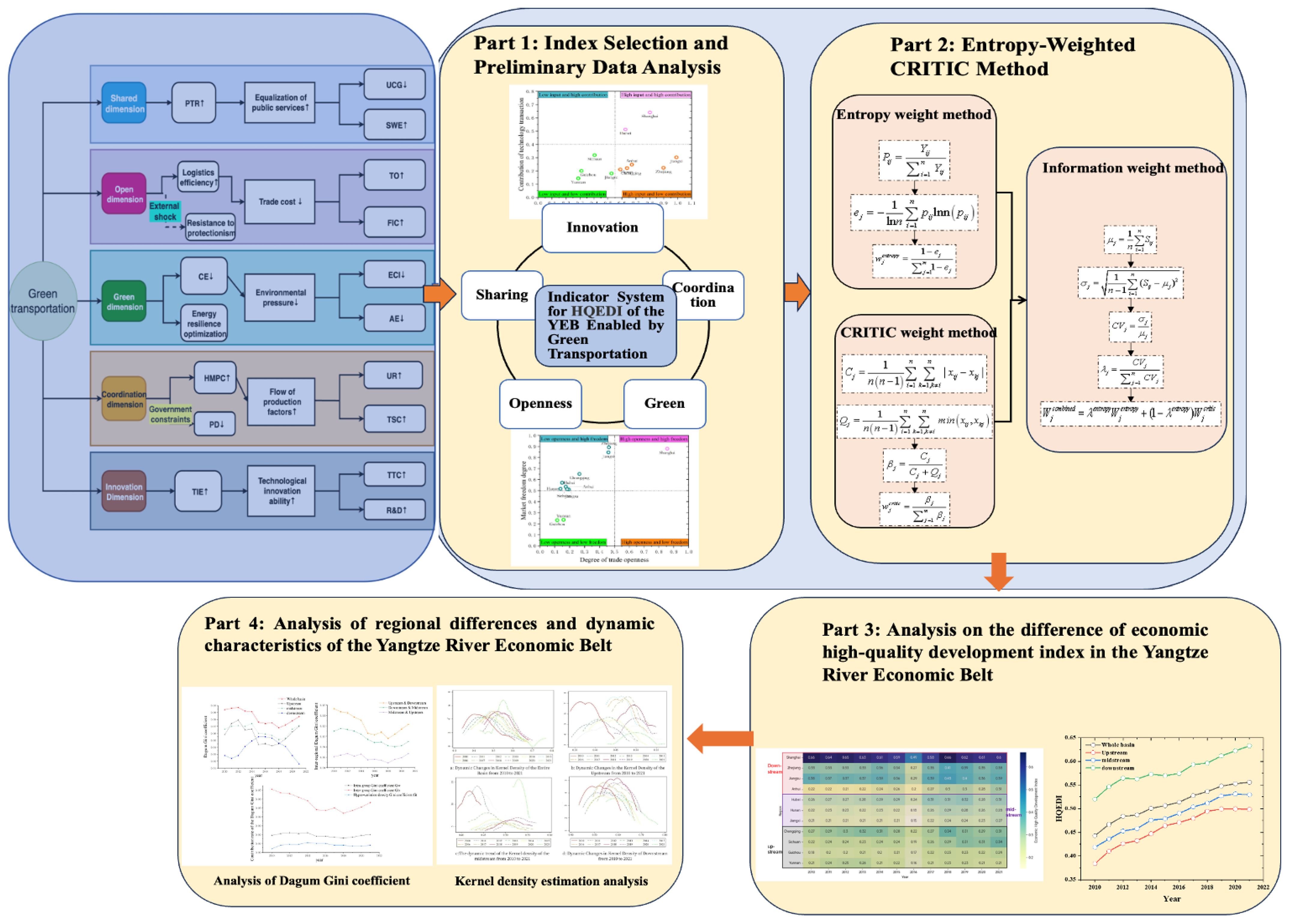
2. Methodology

The construction of the indicator system is grounded in the Theory of New Development Philosophy (innovation, coordination, greenness, openness, sharing), which conceptualizes high-quality development as a multidimensional transition from extensive growth to innovation-driven sustainability. Specifically:

(1)

The entropy weight method is applied based on Information Entropy Theory [34], quantifying data dispersion to avoid subjective bias in weight assignment;

(2)

The CRITIC weight method follows Statistical Contrast Intensity and Conflict Analysis [35], optimizing weights through inter-indicator correlations;

(3)

Their integration balances data variability and indicator independence, aligning with the systemic principle of regional development evaluation.

2.1. Entropy-Weighted CRITIC Method

In order to more comprehensively measure the high-quality development index of regional economy, this study combines the entropy weight method and CRITIC weight method to form a fusion method through the information weight method, that is, the entropy-weighted CRITIC method based on the information weight method. It combines the entropy weighting method to reflect the amount of data information and the CRITIC weighting method to consider the correlation between data, which can reduce subjectivity, reflect the preference of decision makers more comprehensively, balance the fluctuation and correlation of data, and improve the accuracy of weight allocation [26]. The entropy weight method is fundamentally grounded in information theory, specifically the concept of information entropy introduced by Claude Shannon. Information entropy quantifies the uncertainty or disorder inherent in a system or a set of data. In the context of multi-indicator evaluation, the core principle of the entropy weight method is that the weight assigned to an indicator should be proportional to the amount of useful information it provides for distinguishing between the evaluated objects (e.g., provinces).

The key logical steps are as follows:

(1)

Information Content: An indicator that exhibits significant variation across different evaluated objects carries more discriminative information. If all objects have nearly identical values for a particular indicator, that indicator provides little useful information for distinguishing between them.

(2)

Entropy as a Measure of Uncertainty: The entropy value ($e_j$) calculated for an indicator (Equation (2)) inversely reflects the amount of information it provides. A lower entropy value indicates less uniformity (i.e., higher variation) in the data for that indicator across the evaluated objects. This implies higher uncertainty reduction or more useful information contributed by that indicator.

(3)

Weight Assignment: Consequently, indicators with lower entropy (higher variation, more information) should be assigned higher weights in the composite index, as they play a more significant role in differentiating the performance of the evaluated objects. Conversely, indicators with higher entropy (lower variation, less information) receive lower weights. This process is inherently objective, as the weights are derived solely from the intrinsic variability within the dataset itself, minimizing subjective bias.

Therefore, the entropy weight method serves as an objective mechanism to determine indicator importance based on their inherent informational value within the specific dataset under analysis. Its primary goal is to amplify the influence of indicators that effectively differentiate performance while diminishing the influence of those that do not. In this context, the term “evaluated object” refers to the 11 province-level regions (provinces or municipalities) within the YEB. These are Shanghai, Jiangsu, Zhejiang, Anhui, Jiangxi, Hubei, Hunan, Chongqing, Sichuan, Guizhou, and Yunnan. The total number of evaluated objects n is 11. The specific steps of the information weight method combined with the entropy weight method and the CRITIC weight method are as follows:

First, it is necessary to calculate the weight of entropy weight method $w_j^{entropy}$:

$$P_{ij}={\displaystyle \frac{Y_{ij}}{{\sum }_{i=0}^n{Y}_{ij}}}$$

(1)

In Equation (1), i denotes the i-th province-level region ($i=\mathrm{1,2},\dots ,11)$, and j denotes the j-th evaluation indicator, represents the proportion of the $P_{ij}$ evaluated object in the $i$ evaluation index, and $n$ is the total number of evaluated objects. According to Information Entropy Theory, the entropy value $e_j$ of indicator j is calculated as follows:

$$e_j=-{\displaystyle \frac{1}{\ln n}}\sum _{i=1}^n{p}_{ij}\ln \left(p_{ij}\right)$$

(2)

In Equation (2), $e_j$ is the entropy value of the $j$ evaluation index, and is the total number of evaluated objects. A smaller $e_j$ indicates higher data dispersion, thus assigning a higher weight (as it provides richer discriminatory information). Then, the $n$ weight coefficient is calculated:

$$w_j^{entropy}={\displaystyle \frac{1-e_j}{{\sum }_{j=0}^{m}1-e_j}}$$

(3)

In Equation (3), $w_j^{entropy}$ is the weight coefficient of the $j$ evaluation index based on the entropy weight method, and $m$ is the total number of evaluation indexes.

Secondly, it is necessary to calculate the weight of the CRITIC weighting method $w_j^{critic}$:

The full name of the CRITIC weighting method is the Critical Thinking Weighting Method, which is a weight determination method [35] developed based on multi-attribute utility theory. The core idea of this method is to determine the weight by evaluating the conflict and complementarity among various indicators, aiming to reduce the influence of subjective judgment on the weight assignment and improve the objectivity and accuracy of the evaluation results. The specific calculation process is as follows:

Calculation of conflict index: Conflict refers to the inconsistency between evaluation indicators, which can be calculated by the following formula:

$$C_j={\displaystyle \frac{1}{n(n-1)}}\sum _{i=1}^n\sum _{k=1,k\ne i}^n\left|x_{ij}-x_{kj}\right|$$

(4)

In Equation (4), $C_j$ is the conflict of the $j$ evaluation index and $n$ is the number of evaluation objects.

Calculate the complementarity of indicators: Complementarity refers to the interdependence between evaluation indicators, which can be calculated by the following formula:

$$Q_j={\displaystyle \frac{1}{n(n-1)}}\sum _{i=1}^n\sum _{k=1,k\ne i}^{n}min(x_{ij}-x_{kj})$$

(5)

In Formula (5), $Q_j$ is the complementarity of the $j$ evaluation indicator and the weight of the indicator is calculated.

According to the conflict and complementarity, Equation (6) can calculate the weight of each evaluation indicator ${\beta }_j$, and the formula is as follows:

$${\beta }_j={\displaystyle \frac{C_j}{C_j+Q_j}}$$

(6)

Normalization is carried out through Equation (7); since the sum of the weights should be equal to 1, the calculated weights need to be normalized.

$$w_j^{critic}={\displaystyle \frac{{\beta }_j}{{\sum }_{j=1}^m{\beta }_j}}$$

(7)

In Equation (7), $w_j^{critic}$ is the weight of the $j$ evaluation index obtained based on the CRITIC weighting method, and $m$ is the number of evaluation indexes.

Through the above steps, the entropy weighting method mainly determines the weight based on the information provided by the index, namely the entropy value, while the CRITIC weighting method considers the standard deviation (variability) of the index and the correlation between the indicators to determine the weight. Although the CRITIC method can consider the correlation of the indicators, it needs a large amount of data. The entropy weight method determines the weight based on the amount of information contained in the data, but it cannot fully consider the interaction between the indicators.

Finally, the two types of methods are combined by the information weight method to form a fusion method, that is, the entropy-weighted CRITIC method based on the information weight method. In order to measure the regional economic high-quality development index more comprehensively, this paper adopts the information weight method by integrating the advantages of the entropy weight method and the CRITIC method. This method, also known as the coefficient of variation method, is an objective weighting method [36]. The specific steps are as follows:

Step 1: Calculate the mean ${\mu }_j$. For the comprehensive evaluation score of the CRITIC and entropy weight method $S_{ij}$, the mean value is calculated as follows:

$${\mu }_j={\displaystyle \frac{1}{n}}\sum _{i=1}^n{S}_{ij}$$

(8)

In Equation (8), $S_{ij}$ is the value of the $i$ evaluation object on the $j$ evaluation index, and $n$ is the total number of evaluation objects.

Step 2: Calculate the standard deviation ${\sigma }_j$. For the same evaluation index $S_{ij}$, the standard deviation is calculated by Formula (9):

$${\sigma }_j=\sqrt{{\displaystyle \frac{1}{n-1}}\sum _{i=1}^n{(S_{ij}-{\mu }_j)}^2}$$

(9)

Step 3: Calculate the coefficient of variation $C{V}_j$. The coefficient of variation is the ratio of the standard deviation to the mean, which is calculated in Formula (10) as follows:

$$C{V}_j={\displaystyle \frac{{\sigma }_j}{{\mu }_j}}$$

(10)

Step 4: Normalization. The coefficient of variation of all indicators is normalized to obtain the weight of each indicator ${\lambda }_j$. The normalization formula is as follows:

$${\lambda }_j={\displaystyle \frac{C{V}_j}{\sum _{j=1}^{n}C{V}_j}}$$

(11)

In Equation (11): $n$ is the total number of evaluation indicators.

Step 5: Calculate the comprehensive weight of the entropy-weighted CRITIC method $w_j^{combined}$:

$$w_j^{combined}={\lambda }^{entropy}{w}_j^{entropy}+(1-{\lambda }^{entropy}) w_j^{critic}$$

(12)

2.2. Dagum–Gini Coefficient Method

Dagum proposed a decomposition method in 1997, which decomposes the Gini coefficient into within-region disparity $G_w$, between-region group disparity $G_{nb}$, and the contribution of super-density variation $G_t$. In order to compare the differences of the HQEDI in the YEB more reasonably and objectively, this paper divides the eleven provinces and cities into three regions: upstream, middle, and downstream. The decomposition steps and formulas of the Dagum–Gini coefficient method are as follows:

Total Gini coefficient $G$: The total Gini coefficient is an indicator to measure the overall development balance of high-quality economic development in the YEB, which is calculated as follows:

$$G={\displaystyle \frac{1}{2n^2}}\sum _{i=1}^n\sum _{j=1}^n\left|y_i-y_j\right|$$

(13)

where $y_i$ and $y_j$ are the HQEDI of the $i$ and the $j$ regions, respectively. G is normalized by $2n^2$ rather than the conventional $2n$ scaling for microdata. When applied to macro-regional units (e.g., 11 provinces), its value tends to be substantially lower than individual-level Gini indices. Similar low-range values (0.1–0.3) are consistently reported in inter-provincial inequality studies [37].

The Gini coefficient $G_w$ is decomposed into the contribution degree of hypervariable density of intra-regional difference $G_{nb}$ and inter-regional difference $G_t$, and the calculation formula is as follows:

$$G_t=G-G_w-G_{nb}$$

(14)

where $G_t$: hypervariable density represents the part of inequality in addition to the differences within and between regions. $G$: Total Gini coefficient. $G_w$: Gini coefficient of within-region differences. $G_{nb}$: Gini coefficient of inter-regional differences. Therefore, high-quality development achieves “making the cake bigger” through TFP enhancement, while low-quality development (as mentioned in Section 2.3) falls into the “resource curse trap” due to extensive capital investment. The two constitute the theoretical opposite of the development model.

2.3. Kernel Density Method

Kernel density estimation is a non-parametric technique used to flexibly estimate the probability density of random variables, especially when dealing with data with non-standard distributions. This method shows the distribution of the data by smoothing the curve, so as to reveal its evolution trend [38]. In this paper, the Gaussian kernel function is chosen for estimation, which can describe the dynamic trend of spatial and temporal distribution of variables in detail, especially the X trend of absolute difference of random variables. It $f\left(X\right)$ is assumed that $X$ is the density function of random variables, and the formula is:

$$f\left(X\right)={\displaystyle \frac{1}{nh}}\sum _{i=1}^{n}K\left({\displaystyle \frac{X_i-\overline{X}}{h}}\right)$$

(15)

where $X_i$ is a single observation with distribution characteristics, $n$ is the total number of observations, $\overline{X}$ represents the average value of observations, and $h$ represents the bandwidth.

$$K\left(x\right)={\displaystyle \frac{1}{\sqrt{2\pi }}}exp\left(-{\displaystyle \frac{x^2}{2}}\right)$$

(16)

where $K\left(x\right)$ represents the kernel density function.

3. The Calculation and Difference Analysis of the Economic High-Quality Development Index in the YEB

3.1. Indicators and Data

3.1.1. Selection of Indicators

The construction of the index system mainly refers to the research results of Sun [13] and Zhang [12,24] (see

Table 1. Indicator system for the HQEDI of the YEB enabled by green transportation.

Primary Indicator	Secondary Indicators	Indicator Definition	Abbreviation	Data Sources
Innovation	GDP growth rate (+)	Regional GDP growth rate	GDPGR	China Statistical Yearbook https://www.stats.gov.cn/sj/ndsj/ (accessed on 20 April 2025)
	Proportion of R&D investment (+)	R&D expenditure of industrial enterprises above designated size/GDP	R&D	National Science and Technology Statistics Annual Report https://www.sts.org.cn/html/index.html (accessed on 20 April 2025)
	Return on investment (−)	Investment rate/regional GDP growth rate	ROI	Annual Statistical Report on Investment in Fixed Assets https://www.stats.gov.cn/sj/zxfb/202501/t20250117_1958329.html (accessed on 20 April 2025)
	Contribution of technology transactions (+)	Technology trading turnover/GDP	TTC	Annual Report on National Technology Market Statistics http://www.chinatorch.gov.cn/jssc/tjnb/list.shtml (accessed on 20 April 2025)
	Benefits of transportation Investment (+)	Added value of transport industry/fixed investment in transport industry (100 million yuan)	TIE	Yearbook of Transportation Statistics https://www.zgjtnjs.com/ (accessed on 20 April 2025)
Coordination	Consumption structure (+)	Total retail sales of consumer goods/GDP	CS	China Statistical Yearbook https://www.stats.gov.cn/sj/ndsj/ (accessed on 20 April 2025)
	Urbanization rate (+)	Urbanization rate	UR	China Statistical Yearbook https://www.stats.gov.cn/sj/ndsj/ (accessed on 20 April 2025)
	Public debt ratio (−)	Government debt balance/GDP	PD	China Financial Statistics Yearbook https://www.shujuku.org/tag/%E4%B8%AD%E5%9B%BD%E8%B4%A2%E6%94%BF%E5%B9%B4%E9%89%B4/ (accessed on 20 April 2025)
	Contribution of tertiary industry (+)	Increase in the ratio of the output value of the tertiary industry to regional GDP	TSC	China Statistical Yearbook https://www.stats.gov.cn/sj/ndsj/ (accessed on 20 April 2025)
	Highway mileage per capita (+)	Highway mileage/resident population	HMPC	Yearbook of Transportation Statistics https://www.zgjtnjs.com/ (accessedon 20 April 2025)
Green	Energy consumption elasticity index (−)	Energy consumption growth rate/GDP growth rate	ECI	China Energy Statistical Yearbook https://www.stats.gov.cn/zsk/snapshoot?reference=2af5e433078f04afa4dd276ccda961e4_90491BA4193A4D4273403233ED6B1361&siteCode=tjzsk (accessed on 20 April 2025)
	Wastewater volume per unit of output (−)	Wastewater discharge/GDP	WW	China Statistical Yearbook on Environment https://www.shujuku.org/tag/%E4%B8%AD%E5%9B%BD%E7%8E%AF%E5%A2%83%E7%BB%9F%E8%AE%A1%E5%B9%B4%E9%89%B4/ (accessed on 20 April 2025)
	Amount of exhaust gas produced per unit (−)	Sulfur dioxide emissions/GDP	AE	China Statistical Yearbook on Environment https://www.shujuku.org/tag/%E4%B8%AD%E5%9B%BD%E7%8E%AF%E5%A2%83%E7%BB%9F%E8%AE%A1%E5%B9%B4%E9%89%B4/ (accessed on 20 April 2025)
	Per capita transport carbon emissions (−)	Carbon dioxide emissions from transport sector/resident population	CE	China Statistical Yearbook on Environment https://www.shujuku.org/tag/%E4%B8%AD%E5%9B%BD%E7%8E%AF%E5%A2%83%E7%BB%9F%E8%AE%A1%E5%B9%B4%E9%89%B4/ (accessed on 20 April 2025)
Openness	Trade openness (+)	Total imports and exports/GDP	TO	China Customs Statistical Yearbook http://www.customs.gov.cn/customs/302249/zfxxgk/2799825/302274/index.html (accessed on 20 April 2025)
	Contribution rate of foreign investment (+)	Total foreign investment/GDP	FIC	China Statistical Yearbook on Foreign Economic Relations and Trade https://www.shujuku.org/tag/%E4%B8%AD%E5%9B%BD%E8%B4%B8%E6%98%93%E5%A4%96%E7%BB%8F%E7%BB%9F%E8%AE%A1%E5%B9%B4%E9%89%B4/ (accessedon 20 April 2025)
	Market freedom (+)	Regional marketization index	MF	Report on China’s Marketization Index https://baike.baidu.com/item/%E4%B8%AD%E5%9B%BD%E5%88%86%E7%9C%81%E4%BB%BD%E5%B8%82%E5%9C%BA%E5%8C%96%E6%8C%87%E6%95%B0%E6%8A%A5%E5%91%8A(2024)/65661354 (accessed on 20 April 2025)
	Travel activity (+)	Passenger traffic/resident population	MA	Yearbook of Transportation Statistics https://www.zgjtnjs.com/ (accessed on 20 April 2025)
Sharing	Share of labor distribution (+)	Remuneration of workers/regional GDP	LS	China Labor Statistical Yearbook https://www.las.ac.cn/front/book/detail?id=8dbe7daeff2895635813c9ba21f9f630 (accessed on 20 April 2025)
	RGC of residents’ income (+)	Per capita disposable income growth rate/regional GDP growth rate	IGE	China Statistical Yearbook https://www.stats.gov.cn/sj/ndsj/ (accessed on 20 April 2025)
	Urban–rural consumption difference rate (−)	Per capita consumption expenditure of urban residents/per capita consumption expenditure of rural residents	UCG	China Statistical Yearbook https://www.stats.gov.cn/sj/ndsj/ (accessed on 20 April 2025)
	Public welfare expenditure ratio (+)	Proportion of public welfare expenditure in local budget expenditure	SWE	China Financial Statistics Yearbook https://www.shujuku.org/tag/%E4%B8%AD%E5%9B%BD%E8%B4%A2%E6%94%BF%E5%B9%B4%E9%89%B4/ (accessed on 20 April 2025)
	Bus penetration rate (+)	Number of public transport vehicles per 10,000 people (mark platform)	PTR	Yearbook of Transportation Statistics https://www.zgjtnjs.com/ (accessed on 20 April 2025)

R&D expenditure of industrial enterprises above designated size/GDP: According to the standards of the National Bureau of Statistics of China, it refers to industrial enterprises with an annual main business income of ≥20 million yuan (for details, please refer to the compilation instructions of the “China Statistical Yearbook”); Technology trading turnover: It refers to the total amount of contract transactions in the regional technology market, including transaction types such as technology development, transfer, consultation, and services (data sourced from the “Annual Statistical Report of the National Technology Market”). The “science and technology contribution rate” metric is grounded in total factor productivity (TFP) theory. As validated in the World Bank, 2021 [39], technological contribution to sectoral value added serves as a robust proxy for innovation efficiency. Empirical validation comes from the EU Transport Innovation Scoreboard (European Commission, 2023 [40]), where this indicator correlates with patent intensity (r = 0.81, p < 0.01). This study echoes this orientation and measures the economic effectiveness of innovation transformation in the transportation field through TIE. Considering that the data link cannot be used normally outside China, we have provided Supplementary data, as detailed in Table S1.

).

This study presents the “Green Transportation-Enabled Economic High-Quality Development Indicator System for the YEB”, which is grounded in a robust theoretical framework aligned with national strategic directives. The indicator system adheres to the new development philosophy (innovation, coordination, green development, openness, and shared benefits), which is in harmony with the YEB’s strategic focus on “ecology first and green development.” Notably, the system integrates green transportation elements such as transportation investment efficiency, per capita road mileage, and traffic carbon emissions, addressing the gap in existing research regarding the synergy between “transportation, environment, and economy.” The system incorporates 5 primary indicators and 23 secondary indicators, encompassing economic, social, and environmental dimensions. These include innovation metrics (e.g., R&D investment, technology transaction contribution), coordination factors (e.g., urbanization rate, tertiary industry contribution), and green dimensions (e.g., energy consumption elasticity, wastewater discharge intensity). The indicators are designed with positive and negative orientations to reflect the dual constraints of high-quality development. Data for these indicators are sourced from authoritative publications such as the “China Statistical Yearbook,” “China Environmental Statistical Yearbook,” and “Transportation Statistical Yearbook,” ensuring the system’s operational feasibility and the comparability of results. The primary objective of this study is to quantify the multidimensional synergies underlying high-quality development in the YEB, with a focus on identifying the coupling bottlenecks within the “transport-economy-ecology” system. The rationale behind the selection of key indicators is as follows: The Green Transport Index, which measures carbon emissions per unit of GDP, reflects the environmental pressures associated with economic growth and promotes the adoption of low-carbon innovations, such as electric vehicle (EV) usage, in alignment with the Green Development and Decoupling Theory. The R&D Investment Ratio, representing the share of regional expenditure dedicated to research and development, assesses a region’s commitment to transitioning from factor-driven growth to innovation-driven growth, as explained by Endogenous Growth Theory. Lastly, the urban–rural consumption gap, with its narrowing coefficient, serves as an indicator of shared development outcomes, aimed at mitigating regional disparities and ensuring balanced growth, consistent with the Spatial Equilibrium Theory. In addition, we consider urbanization rate a positive indicator (+) based on endogenous growth theory [41], where human capital agglomeration drives innovation. However, the relationship exhibits an inverted-U curve. Beyond 80–85%, diminishing returns may occur due to congestion costs [42]. All provinces in our sample (72–89% UR) remain below this threshold. According to the OECD’s 2022 National Economic Accounting data (https://stats.oecd.org/, accessed on 22 April 2025), the distribution of this indicator in typical consumption-driven economies is as follows: the United States 67.9%, the United Kingdom 63.1%, and Japan 55.2%. The consumption structure (CS) in the downstream area of this study has approached the lower limit of this range (CS$\in$(45–52%)). The urban–rural consumption difference rate (UCG) is defined as the “ratio of per capita consumption expenditure in urban and rural areas”, and the lower the better (approaching 1.0), reflecting the equalization of welfare in urban and rural areas. The relative growth coefficient (RGC) is the ratio of the growth rate of per capita disposable income of residents to the growth rate of regional GDP, reflecting the synchronicity of income growth and economic growth (target value ≥ 1). The adoption of the intensity index (CO₂/GDP) is in line with China’s “dual control” policy (transition from intensity control to total quantity control) because it is directly related to the technological efficiency of regional emission reduction. The results analysis of the index system is detailed in Section 3.1.2.

After collecting and calculating the relevant index data, we used SPSS software (SPSS 23.0) to conduct a preliminary descriptive statistical analysis of the indicators. The statistical results revealed significant differences among the regions of the YEB. To further explore the potential information in the index data, we created a scatter plot depicting the types of innovation and openness in eleven provinces and cities along the YEB, from the two dimensions of innovation and openness.

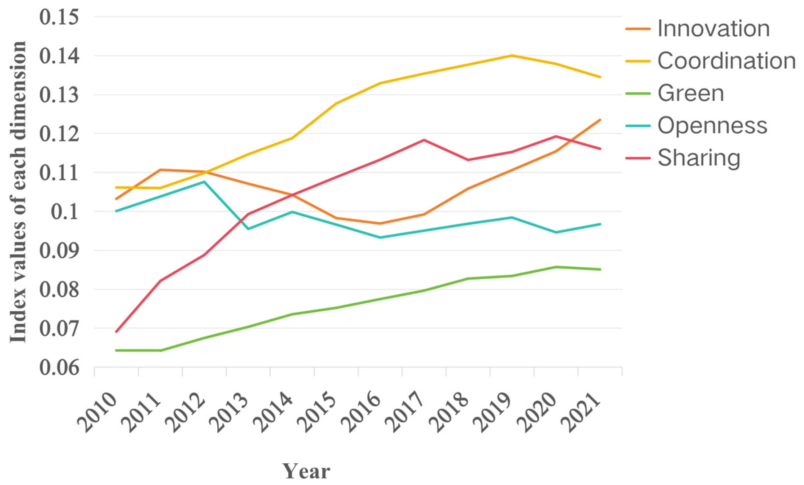
3.1.2. Analysis of Index Data

From the perspective of innovation (see Figure 2), only Shanghai and Hubei fall under the category of high input and high contribution in innovation. This may be attributed to the continuous investment and substantial policy support for scientific and technological R&D and innovation in these regions. On the other hand, Chongqing, Hunan, Anhui, Zhejiang, and Jiangsu fall under the category of high input and low contribution. This suggests that while these provinces have made significant investments in R&D, there is still room for improvement in their innovation outcomes [43].

Finally, Yunnan, Guizhou, Sichuan, and Jiangxi fall into the category of low input and low contribution. Yunnan’s low input and contribution in the innovation dimension are related to its specific economic positioning and developmental stage. Notably, no province in the YEB has yet reached the stage of low input and high contribution in innovation. This may be due to the substantial investment costs of innovation research, whose economic contributions require time to fully manifest. This also indicates that the YEB has a substantial economic base, where traditional enterprises and technologies still account for a significant portion of the total economic benefits, causing the growth of technology transaction contributions to lag behind the overall economic growth. Referring to Figure 2 and Table 1, we can conclude that insufficient upstream openness (e.g., Yunnan and Guizhou) inhibits the transformation of innovation. The Highway Mileage Per Capita (HMPC) indicator in Table 1 suggests that the green transportation coverage rate (PTR) significantly affects coordination.

From the perspective of the openness dimension (see Figure 3), Shanghai is the only province in the first quadrant where both trade openness (TO) and market freedom (MF) exceed 0.5, indicating that its trade openness and market liberalization have reached a high level. This phenomenon is likely closely related to Shanghai’s role as the frontier of China’s opening-up and as an international financial center. The second quadrant includes provinces with high market freedom but relatively low trade openness. In the YEB, most provinces, except for Shanghai, Yunnan, and Guizhou, are located in this quadrant. This indicates that these regions have made progress in promoting market mechanism liberalization but still need further efforts in trade openness.

Notably, Zhejiang and Jiangsu have TO and MF values that are relatively close, and their positions in the coordinate system are nearer to the first quadrant. This may suggest that these two provinces exhibit a strong synergistic effect in trade openness and market liberalization, with significant development potential. Guizhou and Yunnan are both located in the third quadrant, characterized by low trade openness and market freedom. It is noteworthy that in the fourth quadrant, which represents high trade freedom but low market freedom, no region in the eleven provinces and cities along the YEB is located. This phenomenon may be related to the specific economic policies and market environments of each province. It also suggests that while promoting trade liberalization, enhancing market freedom requires more policy support and institutional innovation [44].

3.2. Analysis of the Difference in Economic High-Quality Development Index in the YEB

3.2.1. Analysis of the Difference in Economic High-Quality Development Index at the Provincial Level

In addition, there are significant differences in the levels of high-quality economic development across the Yangtze Economic Belt (YEB) and its upper, middle, and lower reaches, showing a clear pattern of stronger development in the east compared to the west. Specifically, the development trend follows the order lower reaches > middle reaches > upper reaches. Notably, the development trend in the middle reaches mirrors the overall spatial pattern of the YEB (see Figure 4). Additionally, from 2010 to 2021, the high-quality economic development index (HQEDI) of each region within the YEB reveals a general trend of progressive improvement. Over these twelve years, while provinces and cities have seen enhancements in their high-quality economic development levels, the progress has not been uniform, displaying significant regional imbalances. For instance, the HQEDI of downstream regions such as Jiangsu, Shanghai, and Zhejiang is generally high and stable [45], with Shanghai reaching an index value of 0.768 in 2021, the highest in the entire basin. In contrast, upstream regions like Guizhou and Yunnan have relatively low index values. However, provinces such as Hubei, Hunan, and Sichuan in the middle and upper reaches, despite starting from a low base, have shown rapid growth and are gradually closing the gap with the downstream regions. Overall, the average HQEDI of the entire YEB increased from 0.4428 in 2010 to 0.5558 in 2021, reflecting improvements in high-quality economic development across the YEB. These trends indicate that while the YEB has made progress in promoting high-quality economic development, further efforts are needed to ensure coordinated and balanced development among regions for more comprehensive progress.

3.2.2. Analysis of Differences in HQEDI at the Regional Level

According to the division of the YEB by the Office of the Leading Group for Promoting the Development of the YEB, the change trend of the HQEDI in the whole basin, and the upper, middle, and lower reaches of the YEB, from 2010 to 2021 is drawn by data statistics of the calculation results.

The change trend of the HQEDI in the YEB is analyzed to further study its characteristics (see Figure 5). As shown in Figure 4, from 2010 to 2021, the entire YEB basin, including its upper, middle, and lower reaches, generally exhibits a steady growth trend. The average HQEDI value downstream over the 12 years is approximately 0.58, while the upstream average during the same period is about 0.46. The upstream region has the highest annual growth rate, of around 2.43%.

Analyzing the five dimensions, including innovation and coordination (see Figure 6), the period from 2010 to 2021 is divided into four phases. From 2010 to 2012, the development in the green and sharing dimensions is relatively weak, whereas the innovation, coordination, and openness dimensions show high development levels. Growth in the openness dimension tends to stagnate or even reverse. This may be due to large-scale public health emergencies, the current counterflow of economic globalization, and the prevalence of protectionism and unilateralism in some countries, which hinder the normal development of the openness dimension. In response, the Chinese government has proposed a new development pattern, focusing on the major domestic cycle while reinforcing it with dual domestic and international cycles. This strategy actively expands the domestic market, addresses the pain points and blockages in the major domestic cycle, and supports open international development through steady domestic market growth.

4. Analysis of Regional Differences and Dynamic Characteristics of the YEB

4.1. Analysis of Dagum–Gini Coefficient

The HQEDI data of the Yangtze Economic Belt (YEB) from 2010 to 2021 reveal moderate inequality in the region’s high-quality economic development, with overall differences remaining relatively limited (see Figure 7). As shown in Figure 7a, the Dagum–Gini coefficient fluctuates between 0.068 and 0.094, indicating a moderate level of inequality. The coefficient follows a U-shaped trend, reaching its lowest point in 2018 before rising again. This pattern is consistent across the YEB, including both upstream and downstream regions. The highest HQEDI differences occurred in 2011 and 2014, after which they gradually decreased. In contrast, the Gini coefficient for the middle reaches of the Yangtze River exhibits an inverted U-shape, peaking in 2015 and then declining, reaching its lowest point by 2021. Figure 7b highlights fluctuations in economic disparities between different regions. In 2010, the inter-regional Gini coefficient between upstream and downstream reached 0.153, a relatively high value in provincial-scale studies (see Section 4.1 for the methodological rationale), indicating pronounced disparities compared to other regional pairs. From 2011 to 2018, the overall Gini coefficient showed a downward trend, indicating a narrowing of economic differences between regions. However, between 2019 and 2021, the Gini coefficients for the upstream and downstream regions rose once again.

From 2010 to 2021, the overall distribution of high-quality economic development in the YEB was characterized by the following hierarchy of regional disparities: upstream-downstream > downstream-middle reaches > midstream-upstream. This trend remained largely stable, suggesting a spatially unbalanced distribution with higher levels of development in the upstream and downstream areas and lower levels in the middle reaches.

Figure 7(c) presents the decomposition of the Dagum–Gini coefficient, revealing that from 2012 to 2021, the within-group Gini coefficient and the super-variable density Gini coefficient remained relatively low, while the between-group Gini coefficient followed a U-shaped trajectory, fluctuating with development trends. The within-group Gini coefficient (Gw) remained stable and low, indicating minimal economic disparities within regions. In contrast, the between-group Gini coefficient (Gb) fluctuated significantly, reaching 0.058 in 2014, highlighting the substantial impact of regional economic disparities on overall inequality. By 2018, this coefficient decreased to 0.044, suggesting a reduction in regional disparities. Although the super-variable density Gini coefficient (Gt) remained small, it peaked at 0.01 in 2015 before declining, indicating that extreme economic disparities had a limited, though noteworthy, impact on overall inequality. Overall, while economic differences within regions are small, disparities between regions are the primary contributors to the overall economic inequality in the YEB.

Additionally, spatial autocorrelation (such as Moran’s I) can theoretically reveal geographical clustering. Our preliminary test concluded that the p-value of the HQEDI distribution (n = 11 provinces) was approximately 0.5 (not listed here), indicating no significant deviation from spatial randomness. This is consistent with the Gini coefficient for inter-provincial differences driven by non-spatial factors such as institutional heterogeneity or sectoral composition.

4.2. Kernel Density Estimation Analysis

The Dagum–Gini coefficient examines the decomposition results of transportation efficiency differences in the YEB from a perspective of relative differences. This paper analyzes the distribution characteristics and evolution of the HQEDI in the YEB from 2010 to 2021 from a perspective of absolute differences (see Figure 8).

The kernel density estimation method is employed to analyze HQEDI data across the YEB from 2010 to 2021, revealing dynamic changes in regional differences. The analysis indicates an overall growth trend in the HQEDI, with the kernel density curve shifting to the right, signifying steady improvement in economic quality. Over the 12 years, the HQEDI distribution demonstrates a right-skewed feature, with a higher kernel density function value in the median range (0.4 to 0.7) and a lower density in the low range (0 to 0.4), although higher than in the high range (0.7 to 1.0). This suggests that while high-quality economic development is growing, the growth rate remains slow.

Changes in the kernel density curve show a continuous rise in the peak value and an overall shift to the right, indicating improvements in the economic quality index and an increase in the affected areas. In 2010, most regions had an HQEDI around 0.4, whereas by 2021, the HQEDI of most regions had increased to around 0.55, signifying reduced spatial imbalance and progress among less developed regions. The kernel density curve evolves from a wide peak to a sharp peak, with an expanded variation interval and extension into the high-value region, indicating a diffusion trend towards higher quality development and a gradual narrowing of absolute regional differences.

Further analysis of the dynamic evolution of HQEDI differences within the three major rivers reveals significant intra-regional disparities. The kernel density curve for the upstream region was right-skewed, with the main peak shifting rightward from 2010, showing considerable deviation from 2010 to 2011. From 2011 to 2014, the main peak continued shifting rightward, but the kernel density curve flattened, and the peak value remained low, indicating improvements in the economic quality index but substantial overall differences. From 2015 to 2021, the main peak continued its rightward shift; however, the peak value significantly decreased, the distribution width widened, and the range of change expanded, reflecting an increased absolute gap in development levels among provinces and cities in the upstream region.

In the middle reaches, the kernel density curve shifted rightward overall, with an expanded variation interval. From 2010 to 2013, the region experienced rapid advancement in high-quality economic development. From 2014 to 2019, the main peak broadened and decreased, suggesting overall improvement in economic quality but with increasing difficulty in synchronized development among provinces and cities, contributing to absolute differences.

The downstream region’s kernel density curve displayed a bimodal or trimodal distribution with high peak volatility, and the differences have widened in recent years. From 2014 to 2018, the peak value increased and continued shifting rightward. From 2018 to 2021, the peak value significantly decreased and shifted rightward, with an increased variation interval, indicating that while high-quality economic development improved, the absolute differences fluctuated greatly.

5. Conclusions

Based on the new development concept, this paper constructs the measurement and evaluation index system of the Economic High-Quality Development Index (HQEDI) of the YEB from five dimensions, including innovation, coordination, and green transportation empowerment, and draws the following main conclusions:

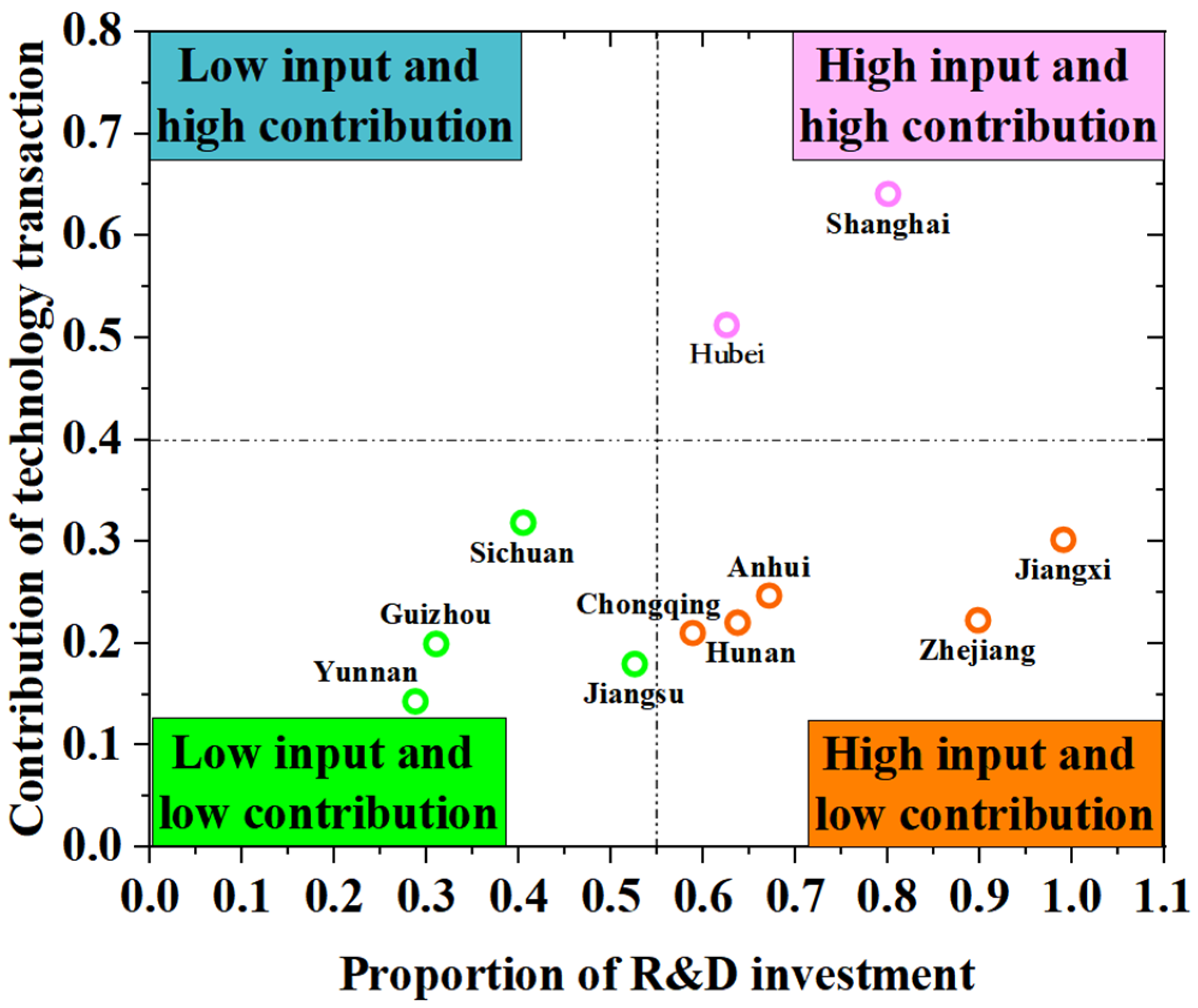
(1)

Contribution of scientific and technological innovation to economic growth: In the dimension of innovation, Shanghai and Hubei exhibit high levels of scientific and technological investment and innovation contribution. Conversely, Chongqing, Hunan, Anhui, Zhejiang, and Jiangsu have high technological investment but relatively low innovation contribution. Yunnan, Guizhou, Sichuan, and Jiangxi show low input and low contribution, with Yunnan’s situation possibly related to its economic positioning and development stage.

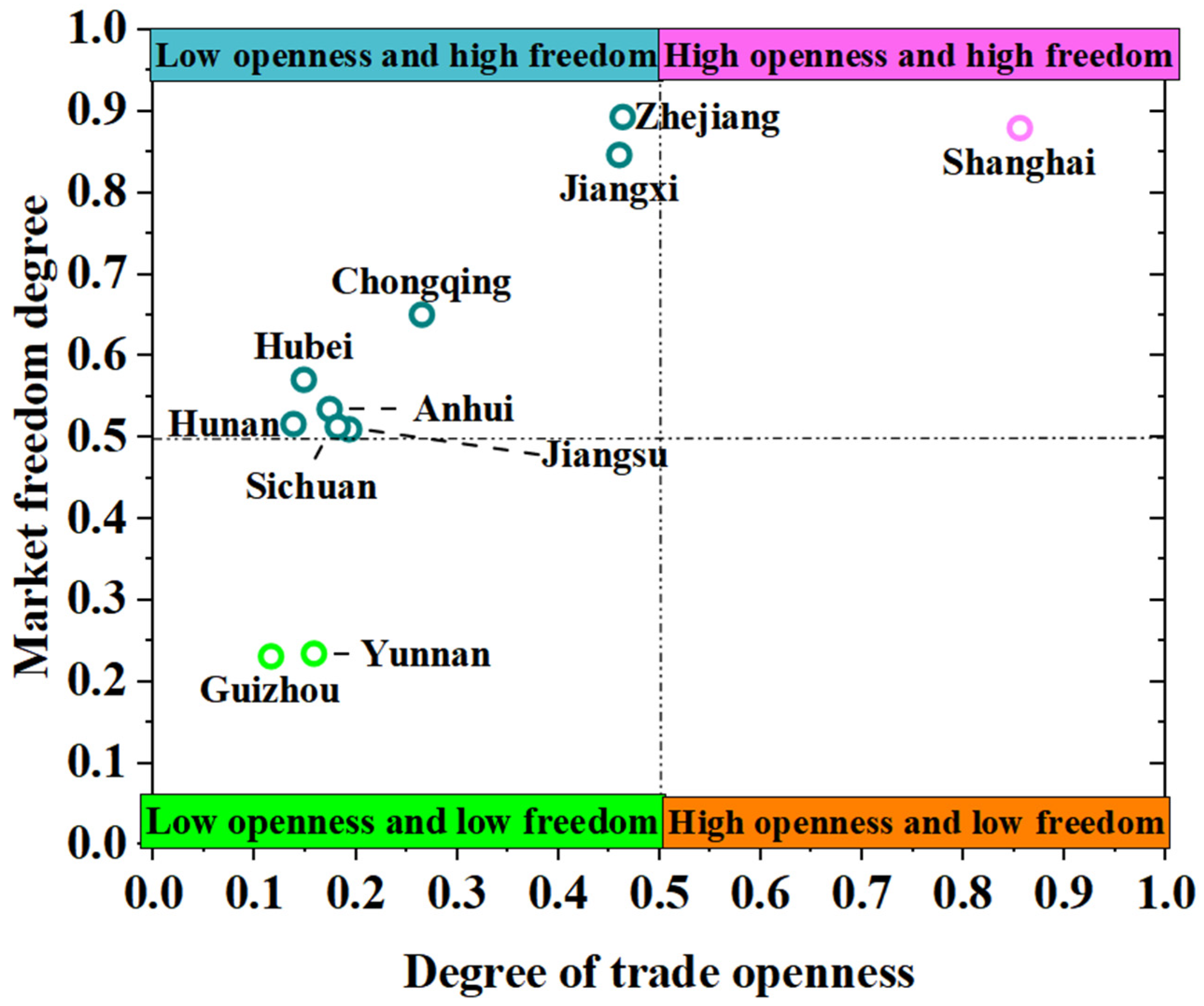
(2)

Trade openness and market freedom: Shanghai excels in trade openness and market freedom, whereas Guizhou and Yunnan lag behind in these indicators. Most provinces and cities boast high market freedom but insufficient trade openness, with Zhejiang and Jiangsu being notable exceptions in terms of trade openness.

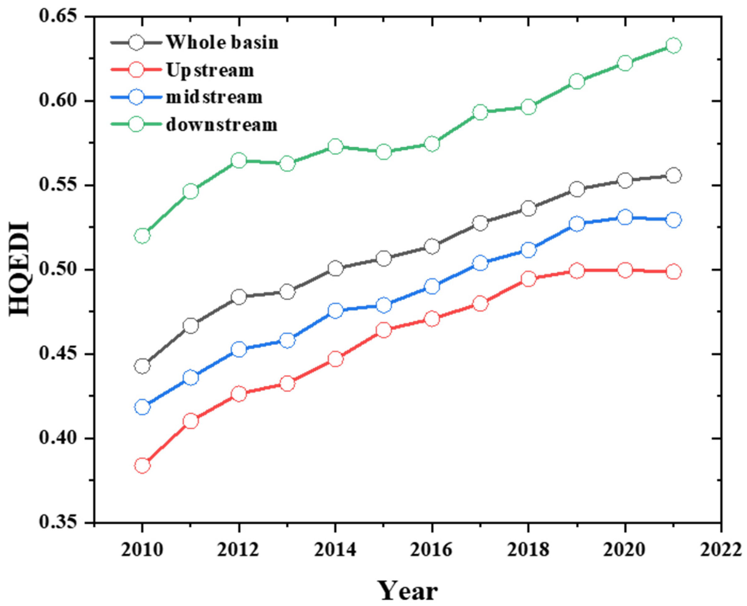
(3)

The YEB (YREB) demonstrates a development pattern of “strong in the east and weak in the west.” The lower reaches, such as Shanghai and Jiangsu, have higher economic development levels. Upstream regions like Sichuan and Chongqing are relatively underdeveloped, while midstream regions such as Hubei and Hunan are intermediate. Overall, HQEDI shows an increasing trend. The average value in downstream regions is higher but grows more slowly, while upstream regions have a faster growth rate.

(4)

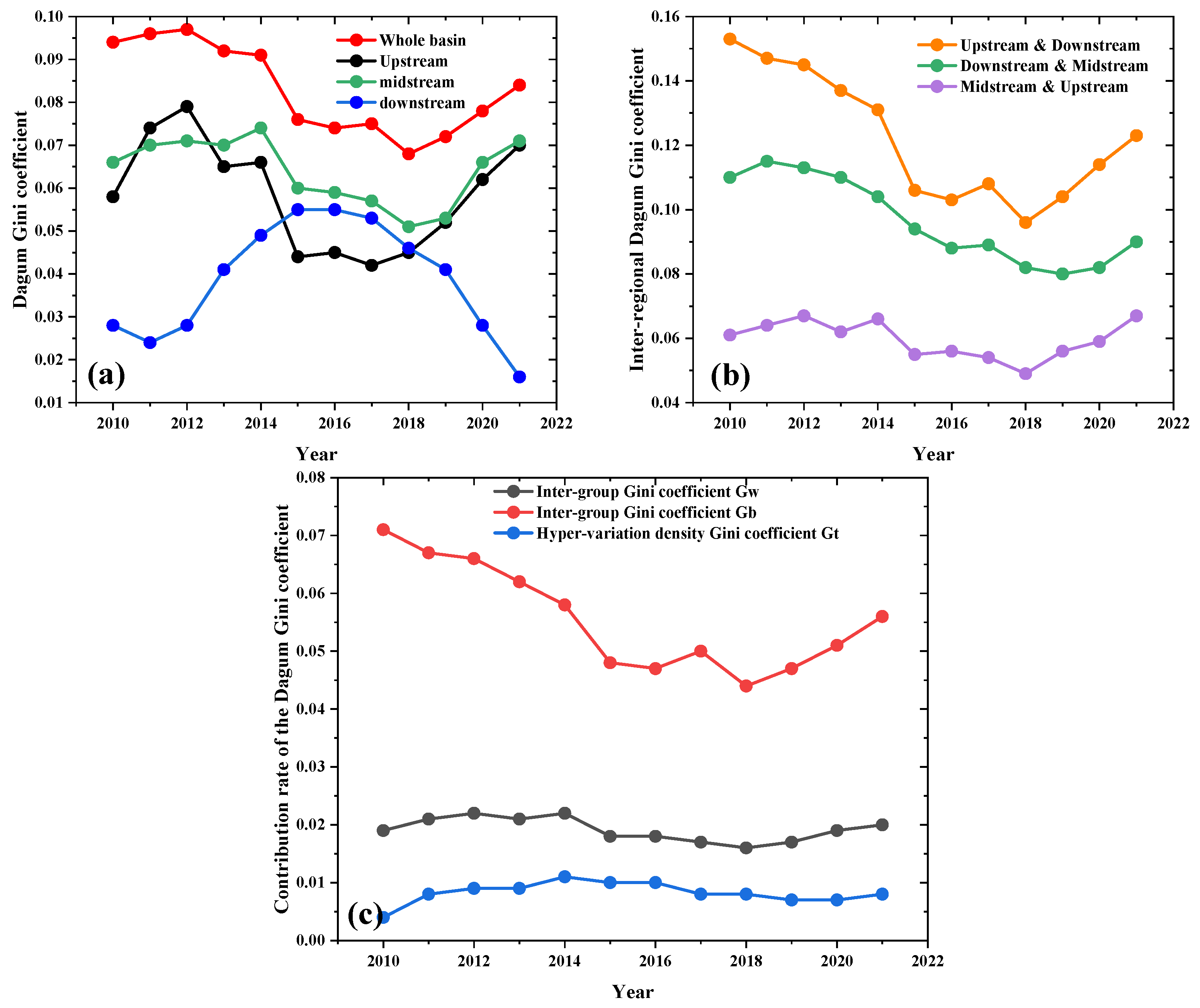
High-quality economic development difference (Dagum–Gini coefficient): Between 2010 and 2021, the overall YEB HQEDI Dagum–Gini coefficient rose from 0.068 to 0.094, showing a U-shaped trend of rising after falling. This indicates that while regional differences in high-quality development exist, overall inequality is low and trending towards narrowing. There is a significant difference between upstream and downstream regions, but this disparity is gradually decreasing over time. The intra-regional Gini coefficient fluctuates less, while the inter-regional Gini coefficient fluctuates more, indicating that economic differences among provinces (cities) within the same region are minor, with disparities among different river basins being the main contributors to overall economic inequality.

(5)

Dynamic characteristics of the kernel density of high-quality economic development: The kernel density curve of the HQEDI in the YEB shifts rightward over time, reflecting improvements in high-quality economic development. However, differences among river basins are evident. The absolute difference in the HQEDI in the upstream region has gradually expanded, showing significant dynamic changes initially and then a steady increase in regional variation. The middle region, after rapid development, currently faces the challenge of increasing absolute differences. The downstream regions continue to improve in high-quality economic development but exhibit strong volatility, with bimodal or trimodal distributions, especially in recent years, indicating a trend of increasing disparity.

6. Limitations and Future Research Directions

6.1. Limitations

This study has methodological, data, and scope limitations. The entropy–CRITIC weighting method, while balancing objectivity and correlation, is sensitive to data distribution (e.g., extreme values) and relies on a linear model (Equation (10)) that oversimplifies complex, nonlinear interactions between green transport and economic systems. Data constraints include a lack of micro-level metrics (e.g., corporate green logistics, smart vehicle rates) due to insufficient provincial statistics, and an inability to fully capture the 3–5-year time-lag effects of green transport investments (e.g., EV infrastructure) within the 2010–2021 dataset. Provincial-level analysis also masks intra-provincial disparities like urban–rural transport gaps.

6.2. Future Research Directions

(1)

Develop Dynamic Weight Models: Use time-varying coefficients (e.g., Markov switching models) to reflect evolving policy impacts on indicator importance.

(2)

Model Nonlinear Interactions: Apply coupling coordination models (e.g., CCD) to quantify synergies/trade-offs between green transport, growth, and equity.

(3)

Incorporate Smart Transport Metrics: Add indicators like highway IoT coverage or multimodal transport integration efficiency to capture digital enablement.

(4)

Assess Ecological Carrying Capacity: Include absolute environmental costs (e.g., total CO₂) alongside intensity indicators to align with IPCC carbon budgets.

(5)

Conduct Cross-Regional Comparisons: Compare the YREB with basins like the Rhine or Mississippi to identify transferable governance strategies.

(6)

Analyze Micro–Macro Linkages: Integrate enterprise-level surveys (e.g., logistics decarbonization) with provincial data to reveal transmission mechanisms.

These directions will enhance the framework’s robustness, scope, and applicability to sustainable transition governance.

7. Policy Recommendations

7.1. Enhance Innovation and Technological Investment

Downstream innovation hubs (e.g., Jiangsu, Shanghai) prioritize market-driven tools like carbon quota auctions and green-tech R&D subsidies, but these are explicitly linked to equity safeguards. For instance, revenue from carbon auctions funds cross-provincial fiscal transfers (≥20% to upstream provinces) to offset regressive impacts on lower-income regions. This resolves the growth–equity trade-off by redistributing decarbonization costs while maintaining innovation incentives.

Midstream industrial transition zones (e.g., Hubei, Hunan) adopt capacity-replacement policies, where coal-fired plant retirements are permitted only if paired with renewable industrial parks generating comparable employment. A “job-carbon swap ratio” (e.g., 1 job created per 500 tons of CO₂ reduced) is enforced via provincial labor–environment co-governance committees, directly addressing the employment–emission reduction trade-off.

Upstream ecological conservation zones (e.g., Yunnan, Guizhou) leverage ecological fiscal transfers, but these are conditioned on SDI-adjusted performance benchmarks. For example, forest carbon sink subsidies increase by 15% if local GDP growth falls below 5%, preventing conservation from exacerbating development gaps.

7.2. Promote Trade Openness and Market Liberalization

Buffer phase (2025–2027): Allow midstream provinces to adopt carbon-intensity targets instead of absolute caps if unemployment exceeds 5%, with the condition that TFP growth compensates for deferred emissions (≥3% TFP rise per 1% intensity relaxation).

Convergence phase (2028–2030): Introduce sectoral carbon budgets but exempt SMEs in upstream regions until per capita GDP reaches USD 10,000, offsetting competitiveness losses via a YREB-wide green supply-chain fund financed by downstream industrial carbon fees.

Neutrality phase (post-2030): Enforce absolute emissions caps but permit inter-provincial carbon credit trading (e.g., Shanghai manufacturers purchasing credits from Sichuan afforestation projects at 1.2× market rate), harmonizing cost efficiency with regional equity.

7.3. A Dynamic Policy Dashboard

Monitoring four dimensions: (1) efficiency (decarbonization cost per ton), (2) equity (rural-urban income Gini coefficient), (3) ecological resilience (wetland restoration ratio), and (4) spillover effects (cross-province green-tech patents)—triggers biannual recalibration if any metric deviates >15% from YREB benchmarks. This embeds scientific resolution of trade-offs into governance, as seen in Jiangsu’s 2023 steel decarbonization pause when automation-driven job losses exceeded predictions.

7.4. Reduce Economic Inequality

While the overall inequality in the YEB has decreased, significant regional disparities still exist, particularly between the upstream and downstream areas. To reduce these disparities, a system of ecological and economic compensation should be established. This could involve redistributing resources from more prosperous regions to those that are less developed, thus encouraging more equitable growth. Additionally, policies to improve education, healthcare, and infrastructure in underdeveloped regions would help address long-term inequalities.

7.5. Strengthen Environmental and Ecological Policies

As the YEB continues to grow, it is crucial to integrate environmental sustainability into the region’s economic development strategies. The adoption of green technologies, particularly in industrial and transportation sectors, should be accelerated. This includes promoting clean energy, green transportation systems, and sustainable industrial practices. Developing an environmental monitoring system based on advanced technologies, such as satellite monitoring and IoT, will help ensure that economic growth does not come at the expense of ecological health.

References

- Deng, M.; Zhang, B.; Wu, C. The Institutional Arrangements and Local Responses for Promoting Green Development of the Yangtze River Economic Belt. Econ. Res. Yangtze River Basin 2024, 1, 99–130. [Google Scholar]
- Kowalski, A.; Nowak, J.; Wiśniewski, T. Transport of goods on the example of a selected section of transport in Poland. Sci. J. Silesian Univ. Technol. Ser. Transp. 2023, 121, 89–102. [Google Scholar]
- Pan, S. Research on the Spatiotemporal Differences and Evolution of Chinese-Style Modernization in the Yangtze River Economic Belt. Resour. Environ. Yangtze Basin 2024, 33, 1369–1381. [Google Scholar]
- Qin, Z.; Huang, B.; Huang, Y. Research on the Construction of Provincial Sub-Center Cities in the Yangtze River Economic Belt. Econ. Res. Yangtze River Basin 2024, 1, 211–241. [Google Scholar]
- Li, Z.; Wu, F.; Zhang, F. A multi-scalar view of urban financialization: Urban development and local government bonds in China. Reg. Stud. 2022, 56, 1282–1294. [Google Scholar] [CrossRef]
- Ball, A.A.; Gouzerh, A.; Brancalion, P.H. Multi-scalar governance for restoring the Brazilian Atlantic Forest: A case study on small landholdings in protected areas of sustainable development. Forests 2014, 5, 599–619. [Google Scholar] [CrossRef]
- Xing, Z.; He, C. Regional Imbalance: Theoretical Review, Research Progress and Future Outlook. Prog. Geogr. 2024, 43, 1839–1852. [Google Scholar]
- Li, S.; Chen, W. Regional carbon inequality and its impact in China: A new perspective from urban agglomerations. J. Clean. Prod. 2024, 480, 144059. [Google Scholar] [CrossRef]
- Yang, J.; Huang, G. Study on the mechanism of multi-scalar transboundary water security governance in the Shenzhen River. Sustainability 2024, 16, 7138. [Google Scholar] [CrossRef]
- Tang, L.; Hu, X.; Luo, Z.; Wei, B.; Wang, Y.; Zhang, Y.; Shao, R.; Chen, C. The Spatiotemporal Coupling of Ecological Fragility and Urbanization Level and Their Interactive Influencing Factors: A Case Study of Hunan Province. Acta Ecol. Sin. 2024, 44, 4662–4677. [Google Scholar]
- Chao, W.; Zhou, W. Analysis of the Evolution and Driving Forces of the Territorial Spatial Pattern of the Middle Reaches Urban Agglomeration in the Yangtze River from the Perspective of Three Zones. Resour. Environ. Yangtze Basin 2024, 33, 1489–1503. [Google Scholar]
- Zhang, X.; Gao, W. Evaluation and Difference Analysis of High-Quality Economic Development. Inq. Econ. Issues 2020, 4, 1–12. [Google Scholar]
- Bo, S.; Zhang, B. Measurement and Analysis of High-Quality Economic Development in Cities Above the Prefecture Level Nationwide. Soc. Sci. Res. 2019, 19–27. [Google Scholar]
- Yu, W.; Rong, J.; Nian, C. Construction and Measurement of High-Quality Economic Development Evaluation System in Inner Mongolia. J. Inn. Mong. Univ. (Nat. Sci. Ed.) 2020, 51, 441–448. [Google Scholar]
- Sun, H.; Gui, Q.; Yang, D. Measurement and Evaluation of High-Quality Economic Development in Chinese Provinces. Zhejiang Soc. Sci. 2020, 8, 4–14. [Google Scholar]
- Tian, H.; Guo, M.; Qin, J. Research on the Impact of Digital Economy on High-Quality Development of the Yangtze River Economic Belt: Evidence from 108 Prefecture-Level Cities. J. Ind. Technol. Econ. 2023, 42, 17–25. [Google Scholar]
- Guo, Y.; Jiang, X.; Zhu, Y.; Zhang, H. Measurement and spatial correlation analysis of high-quality development Level: A case study of the Yangtze River Delta urban agglomeration in China. Heliyon 2024, 10, e29209. [Google Scholar] [CrossRef]
- Zhao, J. How do innovation factor allocation and institutional environment affect high-quality economic development? Evidence from China. J. Innov. Knowl. 2024, 9, 100475. [Google Scholar] [CrossRef]
- Zhang, X.; Zhang, Y.; Zhang, Z. The Measurement, Spatiotemporal Evolution, and Dynamic Spatial Convergence of China’s High-Quality Economic Development Level. Inq. Econ. Issues 2024, 1, 15–37. [Google Scholar]
- Liu, X.; Zhang, X. Research on the evaluation of high-quality development level of green economy in provinces and cities in the Yangtze River Economic Belt based on the five development concepts. For. Econ. 2024, 46, 28–50. [Google Scholar]
- Zhou, Z.; Dai, H.; Zha, Y. Research on the Dilemma and Countermeasures of Digital Transportation Empowering High-Quality Economic Development. China Soft Sci. 2023, 9, 86–94. [Google Scholar]
- Zeng, S.; Fu, Q.; Haleem, F.; Han, Y.; Zhou, L. Logistics density, E-commerce and high-quality economic development: An empirical analysis based on provincial panel data in China. J. Clean. Prod. 2023, 426, 138871. [Google Scholar] [CrossRef]
- Zhao, W.; Xu, X. Digital Economy, Spatial Effect, and High-Quality Economic Development: A Case Study of 110 Cities in the Yangtze River Economic Belt. East. China Econ. Manag. 2023, 37, 42–49. [Google Scholar]
- Zhang, F.; Tan, H.; Zhao, P.; Gao, L.; Ma, D.; Xiao, Y. What was the spatiotemporal evolution characteristics of high-quality development in China? A case study of the Yangtze River economic belt based on the ICGOS-SBM model. Ecol. Indic. 2022, 145, 109593. [Google Scholar] [CrossRef]
- Guo, Y.; Xie, W.; Yang, Y. Dual green innovation capability, environmental regulation intensity, and high-quality economic development in China: Can green and growth go together? Financ. Res. Lett. 2024, 63, 105275. [Google Scholar] [CrossRef]
- Xie, D.; Rong, Y.; Ye, Z. High-Quality Urban Development and Coordinated Urban Agglomeration Development: From the Perspective of Marx’s Differential Rent. Econ. Res. J. 2022, 57, 156–172. [Google Scholar]
- Liu, W.; He, F. Research on the Construction of an Indicator System for High-Quality Development of China’s Economy and Its International Comparative Study. Explor. Econ. Issues 2023, 9, 15–33. [Google Scholar]
- Feng, D.; Li, C.; Deng, S. Study on the Decoupling Effect and Driving Factors of Tourism Transportation Carbon Emissions in the Yangtze River Delta Region. Sustainability 2025, 17, 3056. [Google Scholar] [CrossRef]
- Sen, A. Development as freedom (1999). In The Globalization and Development Reader: Perspectives on Development and Global Change; Wiley-Blackwell: Hoboken, NJ, USA, 2014; pp. 525–562. [Google Scholar]
- OECD. OECD Inclusive Growth Framework; OECD Publishing: Paris, France, 2020. [Google Scholar]
- Romer, P.M. Endogenous Technological Change. J. Political Econ. 1990, 98 Pt 2, S71–S102. [Google Scholar] [CrossRef]
- Stern, D.I. The Rise and Fall of the Environmental Kuznets Curve. World Dev. 2004, 32, 1419–1439. [Google Scholar] [CrossRef]
- North, D.C. Institutions. J. Econ. Perspect. 1991, 5, 97–112. [Google Scholar] [CrossRef]
- Saez, E.; Zucman, G. The Triumph of Injustice: How the Rich Dodge Taxes and How to Make Them Pay; WW Norton & Company: New York, NY, USA, 2019; Chapter 7. [Google Scholar]
- Shannon, C.E. A Mathematical Theory of Communication. Bell Syst. Tech. J. 1948, 27, 379–423. [Google Scholar] [CrossRef]
- Diakoulaki, D.; Mavrotas, G.; Papayannakis, L. Determining Objective Weights in Multiple Criteria Problems: The CRITIC Method. Comput. Oper. Res. 1995, 22, 763–770. [Google Scholar] [CrossRef]
- Ezcurra, R.; Pascual, P.; Rapún, M. The dynamics of regional disparities in Central and Eastern Europe during transition. Eur. Plan. Stud. 2007, 15, 1397–1421. [Google Scholar] [CrossRef]
- Xiang, S.; Qiang, Y. Problems and Paths of Digital Empowerment for the Construction of Urban-Rural Dual Circulation System: A Case Study of Xuancheng City, Anhui Province. J. Yunnan Agric. Univ. (Soc. Sci.) 2022, 16, 72–80. [Google Scholar]
- World Bank. Transport TFP Measurement Guide; World Bank Group: Washington, DC, USA, 2021; p. 38. [Google Scholar]
- European Commission. European Innovation Scoreboard 2023; Publications Office of the European Union: Luxembourg, 2023. [Google Scholar]
- Lucas, R.E. On the mechanics of economic development. J. Monet. Econ. 1988, 22, 3–42. [Google Scholar] [CrossRef]
- Henderson, V. The urbanization process and economic growth: The so-what question. J. Urban. Econ. 2003, 53, 89–112. [Google Scholar]
- Luo, T.; Zhang, Y. A Study on the Coupling Coordination between High-Tech Industry Technological Innovation and Regional High-Quality Economic Development. J. Univ. Shanghai Sci. Technol. 2024, 5, 567–579. [Google Scholar]
- Liu, J. A Study on the Impact of the Digital Economy on High-Quality Economic Development from the Perspective of Efficiency. Ph.D. Thesis, Northwest University, Xi’an, China, 2022. [Google Scholar]
- Li, Y.; Li, C.; Feng, D. Study on Transportation Green Efficiency and Spatial Correlation in the Yangtze River Economic Belt. Sustainability 2024, 16, 3686. [Google Scholar] [CrossRef]