Sustainable Power Coordination of Multi-Prosumers: A Bilevel Optimization Approach Based on Shared Energy Storage

Abstract

Shared energy storage (SES) represents a transformative approach to advancing sustainable energy systems through improved resource utilization and renewable energy integration. In order to enhance the economic benefits of energy storage and prosumers, as well as to increase the consumption rate of renewable energy, this paper proposes a bilevel optimization model for multi-prosumer power complementarity based on SES. The upper level is the long-term energy storage capacity configuration optimization, aiming to minimize the investment and operational costs of energy storage. The lower level is the intra-day operation optimization for prosumers, which reduces electricity costs through peer-to-peer (P2P) transactions among prosumers and the coordinated dispatch of SES. Meanwhile, an improved Nash bargaining method is introduced to reasonably allocate the P2P transaction benefits among prosumers based on their contributions to the transaction process. The case study shows that the proposed model can reduce the SES configuration capacity by 46.3% and decrease the annual electricity costs of prosumers by 0.98% to 27.30% compared with traditional SES, and the renewable energy consumption rate has reached 100%. Through peak–valley electricity price arbitrage, the annual revenue of the SES operator increases by 71.1%, achieving a win–win situation for prosumers and SES. This article, by optimizing the storage configuration and trading mechanism to make energy storage more accessible to users, enhances the local consumption of renewable energy, reduces both users′ energy costs and the investment costs of energy storage, and thereby promotes a more sustainable, resilient, and equitable energy future.

1. Introduction

With the rapid development of distributed PV systems, an increasing number of energy consumers have transformed into prosumers who both consume and produce energy [1,2,3,4]. However, the intermittent and fluctuating nature of PV output makes it poorly matched with the loads of prosumers, which significantly reduces the local consumption level of PV energy [5,6,7]. Equipping the prosumers′ side with energy storage can effectively address this issue, but self-built energy storage by prosumers faces challenges such as high investment costs, long payback periods, and low utilization rates [8,9,10]. Compared with self-built energy storage, SES has diverse sources of funds, effectively reducing users′ investment costs. Moreover, through a shared business model, users can enjoy energy storage services at lower prices, improving the utilization rate of energy storage [11,12,13,14].

At present, researchers have conducted numerous studies on SES. Ref. [15] utilized a MILP (Mixed Integer Linear Programming) model and demand response strategies to schedule the power interaction among distribution networks, SES, and PV prosumers, effectively reducing the electricity cost of PV prosumers and increasing the consumption of PV energy. Ref. [16] conducted configuration planning for community SES based on cooperative game theory between community users and energy storage operators, and verified through simulation that this model could reduce the community′s operating cost by 25.6%. Ref. [17] considered the dual roles of energy storage power stations as both energy suppliers and consumers by establishing a multi-level game model for all stakeholders, and verified through examples that the proposed strategy could effectively balance the interests among energy operators, energy storage operators, and users. Ref. [18] proposed a SES capacity allocation method based on the Stackelberg game, which significantly promoted the collaborative optimization of distribution networks, microgrids, and energy storage power stations, and enhanced the economic benefits for all parties. Ref. [19] proposed a method for optimizing the shared energy storage capacity of wind farms based on cooperative game theory, which effectively reduced the investment cost of energy storage and improved the utilization rate of energy storage. Ref. [20] designed a multi-strategy shared energy storage model. Each user can select the most suitable shared strategy based on the evolutionary game model of multiple strategies. Compared with the traditional shared energy storage model, this model effectively reduces the investment recovery period of energy storage and the energy cost for users. Ref. [21] proposed an energy storage sharing scheme based on the Stackelberg game, which effectively reduced the electricity costs for users. Ref. [22] developed a three-level planning model to optimize the allocation of shared energy storage. The case analysis shows that this model not only enables the rational allocation of energy storage resources but also takes into account the interests of all parties. Ref. [23] proposed an SES optimization allocation method that combines the configuration planning of energy storage power stations with the operation of distributed new energy stations, raising the new energy consumption rate to 100%. Ref. [24] proposed a SES capacity optimization model based on bilevel optimization, improving the utilization rate of SES.

Under the shared business model, P2P transactions can fully leverage the complementarity of energy among different prosumers, effectively increasing the consumption rate of renewable energy and the reliability of energy supply, and prosumers can negotiate transaction prices internally to maximize their own interests [25,26,27,28,29,30]. Ref. [31] utilized SES to achieve P2P transactions between microgrids, significantly improving energy utilization efficiency. Ref. [32] conducted P2P transactions among public buildings equipped with distributed energy resources, enhancing energy sharing among prosumers. Ref. [33] incorporated voltage constraints into the P2P energy trading model and compensated prosumers receiving limit signals to stimulate their participation in the P2P market. Ref. [34] modeled P2P transactions among multiple microgrids using a Stackelberg game model. Ref. [35] focused on commercial buildings with PV systems, obtaining the optimal P2P energy sharing strategy among buildings and reducing operational costs, but lacked further discussion on the distribution of benefits among the trading parties. Ref. [36] proposed a collaborative optimization method for multi-microgrid systems and SES operators by considering P2P transactions among multiple microgrids, but did not plan the scale of energy storage configuration. Ref. [37] designed a P2P transaction mechanism based on credit auctions, and the results showed that P2P transactions did not always bring benefits to prosumers. Ref. [38], by tailoring different pricing plans to suit the varying needs of different consumers, showed that the social welfare of consumers has increased by 49.64%. Ref. [39] proposed an internal pricing model for P2P transactions and solved it using a Mixed Integer Nonlinear Programming (MINLP) model in GAMS. Ref. [40] proposed a two-stage P2P transaction pricing model that combines the advantages of both uniform pricing and differential pricing methods.

A comparison between this article and the above-mentioned literature is shown in

Table 1. Literature comparison.

Literature	Energy Storage Configuration Planning	Optimization of Energy Storage Dispatching	P2P Transactions Between Prosumers	P2P Transaction Price Optimization	Model
[15]	×	√	×	×	MILP
[16]	√	√	×	×	cooperative game
[17]	√	√	×	×	multi-level game
[18]	√	√	×	×	Stackelberg game
[20]	×	√	×	×	evolutionary game model
[33]	×	×	√	×	IEEE 33 bus system
[31]	√	√	√	×	/
[32]	×	√	√	√	Nash bargaining model
[35]	×	√	√	×	/
[36]	×	√	√	√	multi-objective master–slave game
[39]	×	√	√	√	MINLP
[40]	×	×	√	√	ADMM
This article	√	√	√	√	bilevel optimization

“√” indicates that the literature has taken this into account, “×” indicates that the literature did not take this into account, and “/” indicates that it was not mentioned clearly.

.

To sum up, the existing literature on SES mainly focuses on energy storage configuration planning and the optimization of interaction behaviors between energy storage and prosumers as well as distribution networks. However, in the energy storage planning stage, the P2P transactions among prosumers are rarely considered, and the current research on the revenue distribution mechanism of P2P transactions among prosumers is still not perfect. In view of these deficiencies, this paper proposes a bilevel optimization model for multi-prosumer energy complementarity based on SES. This model not only takes into account the interaction behaviors among energy storage, the power grid, and prosumers but also incorporates P2P transactions among prosumers into the optimization scope. The aim is to determine the optimal configuration of energy storage and the optimal operation plans for energy storage and prosumers. Furthermore, this paper also optimizes the P2P transaction prices between prosumers through an improved Nash bargaining method, aiming to achieve a reasonable distribution of benefits among prosumers. In summary, the objectives of this paper are to enhance the economic benefits of energy storage and prosumers, to facilitate the local consumption of renewable energy through the optimized dispatching among energy storage, prosumers, and the power grid, and to optimize the P2P transaction prices of prosumers. The main contributions of this article are as follows:

• A bilevel optimization model for power complementarity among multiple prosumers based on SES has been established. The upper level is the long-term energy storage configuration planning, while the lower level is the intra-day operation optimization considering P2P transactions between prosumers. The bilevel model ensures the interests of both energy storage and prosumers.
• Through a series of transformations, the original bilevel optimization problem is transformed into a single-level mixed integer linear programming problem, enabling the original problem to be solved quickly.
• An improved Nash bargaining revenue distribution model for prosumers was proposed, which made a reasonable distribution of the revenue from P2P transactions among prosumers.

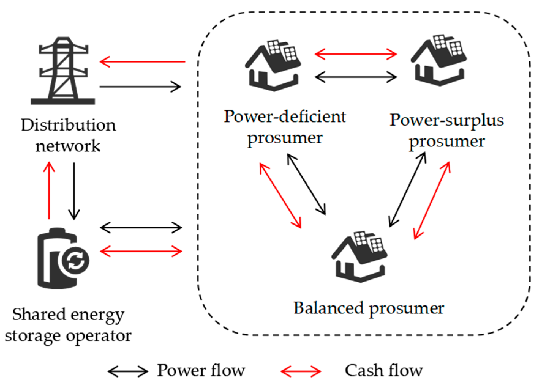
2. Structure of the Multi-Prosumer Power Complementarity System Based on SES

The structure of the multi-prosumer power complementary system based on SES is shown in Figure 1, which includes three types of trading entities: PV prosumers, SES operators, and the distribution network. The SES operator determines the capacity and maximum charging and discharging power of the SES based on the charging and discharging demands of the prosumers, purchases electricity from the distribution network during valley hours, and sells it to the prosumers during peak hours to earn the price difference. At the same time, it charges the prosumers for energy storage services based on the charging and discharging volume. PV prosumers can be classified into three types according to the size of their PV power generation and electricity consumption: power-deficient prosumers, power-surplus prosumers, and balanced prosumers. Taking into account the varying policies for PV power grid connection in different regions and the facts that the current grid connection prices for PV power in most provinces are based on the benchmark price of coal-fired power generation, PV power grid connection is subject to policy restrictions, and yields relatively low returns, this paper assumes that the surplus power of prosumers cannot be connected to the grid. This arrangement is conducive to promoting the local consumption of PV power. Prosumers conduct P2P transactions of electricity based on the complementary relationship of their power generation and electricity consumption in the same period and negotiate the transaction price together to enhance the overall benefit. According to the complementary relationship of prosumers at different times, prosumers can sell the excess PV power to the SES when there is a surplus and purchase electricity from the SES when the PV power is insufficient, thereby increasing the PV consumption rate. The remaining insufficient electricity is purchased from the distribution network to make up for it, reducing the electricity purchase cost. In addition, the P2P transactions between prosumers are conducted through the distribution system network, which undoubtedly increases the operation cost of the grid. Therefore, prosumers must pay a network usage fee to the grid to compensate for its loss.

3. Bilevel Optimization Model for Multi-Prosumer Power Complementarity Based on SES

The bilevel optimization model can simultaneously consider the interests of both the upper and lower levels. The upper level first determines the feasible range of decision variables, and the lower level must optimize within the decision-making scope of the upper level. This simultaneously meets the demands of both levels and maximizes the overall benefit.

3.1. Upper-Level SES Configuration Optimization Model

3.1.1. Objective Function of the Upper-Level Model

The objective of the upper-level model is to minimize the operation cost of the SES, which is responsible for solving the SES capacity and the maximum charging and discharging power. The decision variables include the SES capacity, the maximum charging and discharging power of the SES, the power purchased by the SES from prosumers, the power sold by the SES to prosumers, and the power purchased by the SES from the power grid. The objective function of the upper-level model is

$$\min C_1=C^{inv}+C^{ess,b}+C^{ess,grid,b}-C^{ess,s}-C^{serve}$$

(1)

In the formula, $C^{inv}$ represents the average daily investment and maintenance cost of the SES, CNY; $C^{ess,b}$ represents the cost of purchasing electricity from prosumers by the SES on a typical day, CNY; $C^{ess,grid,b}$ represents the cost of purchasing electricity from the power grid by the SES on a typical day, CNY; $C^{ess,s}$ represents the revenue from selling electricity to prosumers by the SES on a typical day, CNY; and $C^{serve}$ represents the SES service fee on a typical day, CNY.

(1)

The average daily investment and maintenance costs of SES are

$$C^{inv}={\displaystyle \frac{{\delta }_p{P}_{\max }^{ess}+{\delta }_c{E}_{\max }^{ess}}{T_S}}+{\displaystyle \frac{m{P}_{\max }^{ess}}{365}}$$

(2)

In the formula, ${\delta }_p$ represents the unit power capacity cost of SES, CNY/kW; ${\delta }_c$ represents the unit energy capacity cost of SES, CNY/kWh; $P_{\max }^{ess}$ represents the maximum charge and discharge power of the SES, kW; $E_{\max }^{ess}$ represents the maximum capacity of the SES, kWh; $T_s$ represents the operation time of the SES, d; and m represents the unit power operation and maintenance cost of SES, CNY/(a·kW).

(2)

The cost of electricity purchase from prosumers for SES is

$$C^{ess,b}={\displaystyle \sum _{t=1}^{24}{\displaystyle \sum _{u=1}^U{P}_{ess,b}(u,t)}\lambda (t)}$$

(3)

In the formula, $t$ represents the $t$ time period of a day; $u$ represents the Prosumer $u$; $U$ represents the total number of prosumers; $P_{ess,b}(u,t)$ represents the power purchased by the SES from the Prosumer $u$ in the $t$ time period, kW; and $\lambda (t)$ represents the electricity purchase price of the SES in the $t$ time period, CNY/kWh.

(3)

The cost of electricity purchased from the grid for SES is

$$C^{ess,grid,b}={\displaystyle \sum _{t=1}^{24}{P}_{ess,grid,b}}(t)\epsilon (t)$$

(4)

In the formula, $P_{ess,grid,b}(t)$ represents the power purchased by the SES from the grid in the $t$ time period, kW; and $\epsilon (t)$ represents the electricity selling price of the grid in the $t$ time period, CNY/kWh.

(4)

The revenue from electricity sales by SES to prosumers is

$$C^{ess,s}={\displaystyle \sum _{t=1}^{24}{\displaystyle \sum _{u=1}^U{P}_{ess,s}(u,t)}\phi (t)}$$

(5)

In the formula, $P_{ess,s}(u,t)$ represents the power sold by the SES to the Prosumer $u$ in the $t$ time period, kW; and $\phi (t)$ represents the electricity selling price of the SES in the $t$ time period, CNY/kWh.

(5)

Storage service fees charged by SES to prosumers are

$$C^{serve}={\displaystyle \sum _{t=1}^{24}{\displaystyle \sum _{u=1}^U[P_{ess,s}(u,t)}+P_{ess,b}(u,t)}]\theta$$

(6)

In the formula, $\theta$ represents the price of the SES service fee, CNY/kWh.

3.1.2. Upper-Level Model Constraints

(1)

The state of charge and charge/discharge power constraints are

$$E_{ess}(t)=E_{ess}(t-1)+[{\mu }_{abs}{P}_{ess,abs}(t)-{\displaystyle \frac{1}{{\mu }_{relea}}}{P}_{ess,relea}(t)]$$

(7)

$$E_{ess}(1)=20\%E_{\max }^{ess}$$

(8)

$$10\%E_{\max }^{ess}<E_{ess}(t)<90\%E_{\max }^{ess}$$

(9)

$$0<P_{ess,abs}(t)<{\nu }_{abs}(t)P_{\max }^{ess}$$

(10)

$$0<P_{ess,relea}(t)<{\nu }_{relea}(t)P_{\max }^{ess}$$

(11)

$${\nu }_{abs}+{\nu }_{relea}\le 1$$

(12)

$$E_{ess}(24)=20\%E_{\max }^{ess}$$

(13)

In the formulas, $E_{ess}(t)$ represents the remaining energy of the SES in the $t$ time period, kWh; $P_{ess,abs}(t)$ represents the charging power of the SES in the t time period, kW; $P_{ess,relea}(t)$ represents the discharging power of the SES in the t time period, kW; ${\mu }_{abs}$ represents the charging efficiency of the SES; ${\mu }_{relea}$ represents the discharging efficiency of the SES; and ${\nu }_{abs}(t)$ and ${\nu }_{relea}(t)$ are the status bits of the SES charging and discharging, which are 0–1 variables.

(2)

Capacity ratio constraints of SES are

$$E_{\max }^{ess}=\vartheta P_{\max }^{ess}$$

(14)

In the formula, $\vartheta$ represents the SES capacity ratio.

3.2. Optimization Model for Lower-Level Prosumers′ Operation

3.2.1. Objective Function of the Lower-Level Model

The objective of the lower-level model is to minimize the electricity cost for prosumers, and is responsible for solving the optimal operation plan for prosumers, including the power purchased from the grid, the power charged and discharged to the SES, and the power traded among prosumers, etc. It is worth noting that the internal transactions among prosumers bring no benefit to the entire prosumer alliance, and so only the network usage fee paid to the grid is considered during optimization. The objective function of the lower-level model is

$$\min C_2=C^{grid}+C^{ess,s}+C^{serve}+C^{user,grid}-C^{ess,b}$$

(15)

In the formula, $C^{grid}$ represents the cost of electricity purchased by prosumers from the power grid in a typical day, CNY; and $C^{user,grid}$ represents the network usage fee paid by prosumers to the grid in a typical day, CNY.

(1)

The cost for prosumers to purchase electricity from the power grid is

$$C^{grid}={\displaystyle \sum _{u=1}^U{\displaystyle \sum _{t=1}^{24}{P}_{grid}(u,t)\epsilon (t)}}$$

(16)

In the formula, $P_{grid}(u,t)$ represents the power purchased by prosumers from the grid in the t time period, kW.

(2)

Network usage fees paid by prosumers to the power grid are

$$C^{user,grid}={\displaystyle \sum _{u^{\prime }\in U-u}{\displaystyle \sum _{u=1}^U{\displaystyle \sum _{t=1}^{24}\frac{1}{2}[P_{user,b}(u,u^{\prime },t)}}+P_{user,s}(u,u^{\prime },t)]\gamma }$$

(17)

In the formula, $P_{user,b}(u,u^{\prime },t)$ represents the power purchased by the Prosumer $u$ from the Prosumer $u^{\prime }$ in the t time period, kW; $P_{user,s}(u,u^{\prime },t)$ represents the power sold by the Prosumer $u$ to the Prosumer $u^{\prime }$ in the t time period, kW; and $\gamma$ represents the network usage fee price, CNY/kWh.

3.2.2. Lower-Level Model Constraints

(1)

The power balance constraint is

$$P_{pv}(u,t)+P_{grid}(u,t)+P_{ess,s}(u,t)+{\displaystyle \sum _{u^{\prime }\in U-u}{P}_{user,b}(u,u^{\prime },t)}-P_{ess,b}(u,t)-{\displaystyle \sum _{u^{\prime }\in U-u}{P}_{user,s}(u,u^{\prime },t)}-P_{load}(u,t)=0$$

(18)

In the formula, $P_{pv}(u,t)$ represents the PV power generation of the Prosumer u in the t time period, kW; and $P_{load}(u,t)$ represents the load power of the Prosumer u in the t time period, kW.

(2)

The power balance constraints for SES charging and discharging are

$$P_{ess,grid,b}(t)+{\displaystyle \sum _{u=1}^U{P}_{ess,b}(u,t)}=P_{ess,abs}(t)$$

(19)

$${\displaystyle \sum _{u=1}^U{P}_{ess,s}(u,t)}=P_{ess,relea}(t)$$

(20)

(3)

The power balance constraint between prosumers is

$${\displaystyle \sum _{u=1}^U{\displaystyle \sum _{u^{\prime }\in U-u}{P}_{user,b}(u,u^{\prime },t)}}={\displaystyle \sum _{u=1}^U{\displaystyle \sum _{u^{\prime }\in U-u}{P}_{user,s}(u,u^{\prime },t)}}$$

(21)

$$P_{user,b}(u,u^{\prime },t)=P_{user,s}(u^{\prime },u,t)$$

(22)

(4)

The upper and lower limits of constraints on the transaction power between prosumers are

$$0<{\displaystyle \sum _{u^{\prime }\in U-u}{P}_{user,b}(u,u^{\prime },t)}<{\nu }_{user,b}(u,t)P_{user,mutual}^{\max }$$

(23)

$$0<{\displaystyle \sum _{u^{\prime }\in U-u}{P}_{user,s}(u,u^{\prime },t)}<{\nu }_{user,s}(u,t)P_{user,mutual}^{\max }$$

(24)

In the formulas, $P_{user,mutual}^{\max }$ represents the maximum power of transactions between prosumers, kW; and ${\nu }_{user,b}(u,t)$ and ${\nu }_{user,s}(u,t)$ are the state bits of power purchase and sale between prosumers, respectively, which are 0–1 variables.

(5)

The power constraints for electricity purchase and sale between prosumers and SES are

$$0<P_{ess,b}(u,t)<{\nu }_{ess,b}(u,t)P_{ess,user}^{\max }$$

(25)

$$0<P_{ess,s}(u,t)<{\nu }_{ess,s}(u,t)P_{ess,user}^{\max }$$

(26)

In the formulas, $P_{ess,user}^{\max }$ represents the maximum power of transactions between prosumers and the SES, kW; and ${\nu }_{ess,b}(u,t)$ and ${\nu }_{ess,s}(u,t)$ represent the states of the prosumer selling and purchasing electricity from the SES, respectively, and they are 0–1 variables.

(6)

The power purchase constraint of prosumers from the power grid is

$$0<P_{grid}(u,t)<{\nu }_{grid}(u,t)P_{user,grid}^{\max }$$

(27)

In the formula, $P_{user,grid}^{\max }$ represents the maximum power that prosumers purchase from the power grid, kW; and ${\nu }_{grid}(t)$ represents the state of the prosumer purchasing electricity from the grid, which is a 0–1 variable.

(7)

The constraint that prosumers cannot simultaneously purchase and sell electricity is

$$0<or[{\nu }_{ess,b}(u,t),{\nu }_{user,s}(u,t)]+or[{\nu }_{ess,s}(u,t),{\nu }_{user,b}(u,t),{\nu }_{grid}(u,t)]\le 1$$

(28)

In the formula, or [] represents the OR operation.

4. Prosumers′ Revenue Distribution Model Based on an Improved Nash Bargaining Method

Based on the above bilevel optimization model, the transaction electricity among prosumers can be obtained. Since the transaction occurs within the prosumer alliance, the overall benefit of the prosumer alliance to the outside is zero, but the conflicts of interest among the prosumers within the alliance still exist. Therefore, this paper uses an improved Nash bargaining method to allocate the benefits of each prosumer. The traditional Nash bargaining method does not consider the contribution of different participants to the cooperative benefits, which easily leads to an uneven distribution of benefits. This paper measures the contribution of each prosumer based on their transaction volume and uses the bargaining factor to quantify this indicator.

First, calculate the electricity volume of each prosumer participating in the P2P transactions:

$$Q_{user,b}(u)={\displaystyle \sum _{t=1}^{24}{\displaystyle \sum _{u\prime \in U-u}{P}_{user,b}(u,u\prime ,t)}}$$

(29)

$$Q_{user,s}(u)={\displaystyle \sum _{t=1}^{24}{\displaystyle \sum _{u\prime \in U-u}{P}_{user,s}(u,u\prime ,t)}}$$

(30)

In the formula, $Q_{user,b}(u)$ represents the purchased electricity quantity of Prosumer u participating in the transactions among prosumers, kWh; and $Q_{user,s}(u)$ represents the sold electricity quantity of Prosumer u participating in the transactions among prosumers, kWh.

In the transaction process, the seller should have more bargaining power than the buyer [41]. Therefore, this paper adopts a nonlinear mapping function to calculate the bargaining factor of each prosumer:

$${\zeta }_u=e^{{\displaystyle \frac{Q_{user,b}(u)}{Q_{user,b}^{all}}}-1}+e^{{\displaystyle \frac{Q_{user,s}(u)}{Q_{user,s}^{all}}}}-{\displaystyle \frac{1+e}{e}}$$

(31)

In the formula, ${\zeta }_u$ is the bargaining factor of Prosumer u; e is a natural constant; $Q_{user,b}^{all}$ is the total purchased electricity in transactions among prosumers; and $Q_{user,s}^{all}$ is the total sold electricity in transactions among prosumers.

The saved revenue when prosumers conduct transactions compared to when they do not is taken as the optimization objective. When no transactions occur, the excess electricity of prosumers is sold to the power grid, and the insufficient electricity is purchased from the power grid. Then, the objective function is as follows:

$$\min C_3=-{{\displaystyle \prod _{u=1}^U(C_{user,mutual}^{before}(u)-C_{user,mutual}^{after}(u))}}^{{\zeta }_u}$$

(32)

In the formula, $C_{user,mutual}^{before}$ represents the electricity cost when prosumers do not conduct transactions, CNY; and $C_{user,mutual}^{after}$ represents the electricity cost when prosumers conduct transactions, CNY.

(1)

The electricity cost when prosumers do not engage in transactions is

$$C_{user,mutual}^{before}(u)={\displaystyle \sum _{t=1}^{24}{\displaystyle \sum _{u\prime \in U-u}{P}_{user,b}(u,u\prime ,t)}}\epsilon (t)-{\displaystyle \sum _{t=1}^{24}{\displaystyle \sum _{u\prime \in U-u}{P}_{user,s}(u,u\prime ,t)}}\sigma (t)$$

(33)

In the formula, $\sigma (t)$ represents the electricity purchase price of the power grid in the t time period, CNY/kWh.

(2)

The electricity cost during transactions between prosumers is

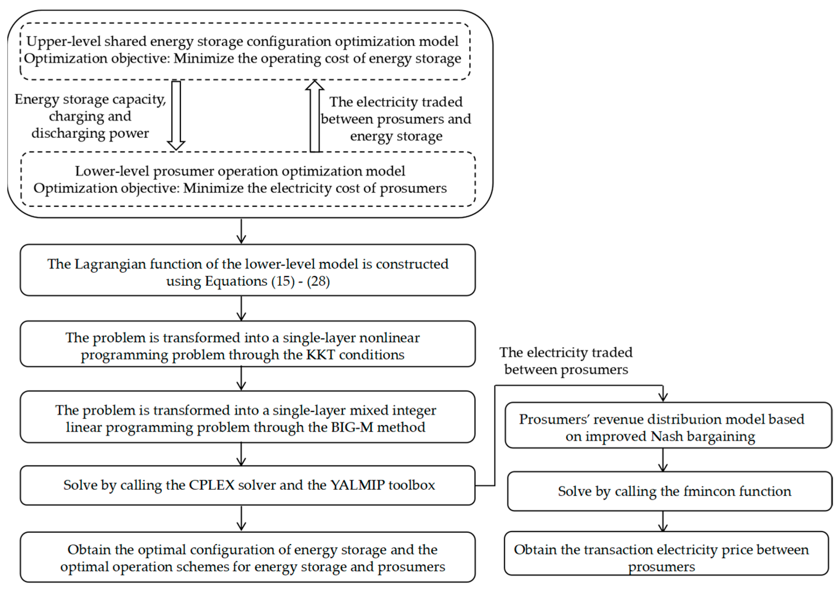
$$C_{user,mutual}^{after}(u)={\displaystyle \sum _{t=1}^{24}{\displaystyle \sum _{u\prime \in U-u}{P}_{user,b}(u,u\prime ,t)}}\tau (u,u\prime ,t)-{\displaystyle \sum _{t=1}^{24}{\displaystyle \sum _{u\prime \in U-u}{P}_{user,s}(u,u\prime ,t)}}\rho (u,u\prime ,t)$$

(34)

In the formula, $\tau (u,u^{\prime },t)$ represents the electricity purchase price from Prosumer $u$ to Prosumer $u^{\prime }$ in the t time period, CNY/kWh; and $\rho (u,u^{\prime },t)$ represents the electricity sale price from Prosumer $u$ to Prosumer $u^{\prime }$ in the t time period, CNY/kWh.

The transaction prices between prosumers need to meet the following constraints:

$$\sigma (t)\le \tau (u,u\prime ,t)\le \epsilon (t)$$

(35)

$$\sigma (t)\le \rho (u,u\prime ,t)\le \epsilon (t)$$

(36)

5. Solution Method

The flowchart of the solution method for the model constructed in this paper is shown in Figure 2. The bilevel model constructed in this paper has nonlinear constraints, and there is a coupling relationship between the upper-level model and the lower-level model, making it difficult to solve directly. Equations (15)–(28) are used to construct the Lagrangian function of the lower-level model, as shown in Appendix A Equation (A1). Next, using the KKT complementary slackness conditions of the lower-level model, the Lagrangian function of the lower-level model is transformed into the additional constraints of the upper-level model, as shown in Appendix A Equations (A2)–(A22). The original problem is thus transformed into a single-level nonlinear optimization problem, as shown in Equations (1)–(14) and Appendix A Equations (A2)–(A22). The Big-M method is used to linearize the nonlinear constraints, as shown in Appendix A Equations (A23)–(A44). The problem is ultimately transformed into a single-level mixed-integer linear programming problem, as shown in Equations (1)–(14) and Appendix A Equations (A2)–(A11) and (A23)–(A44). This way, the problem can be solved by calling the CPLEX solver and the YALMIP toolbox in Matlab R2019b. The specific transformation process is shown in Appendix A. The prosumers′ revenue distribution model based on the improved Nash bargaining method can be directly solved by calling the fmincon function for solving nonlinear programming problems in Matlab R2019b.

6. Case Study Analysis

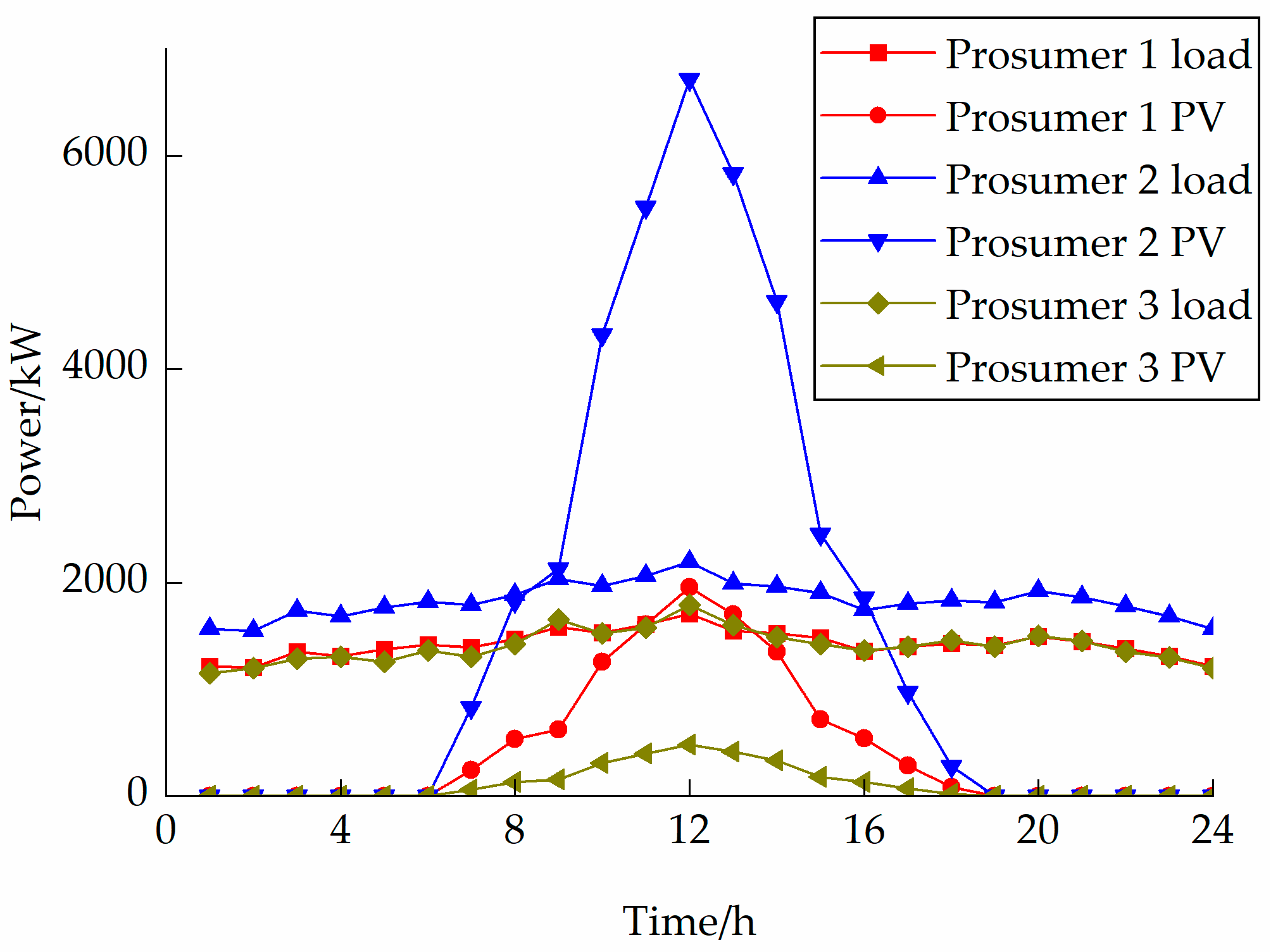
6.1. Basic Data of the Example

This paper takes a multi-prosumer system in a certain area as an example to verify the feasibility of the proposed optimization model. The system includes three prosumers: Prosumer 1 is a balanced prosumer, Prosumer 2 is a power-surplus prosumer, and Prosumer 3 is a power-deficient prosumer. The typical daily electricity load and PV power generation of the prosumers are shown in Appendix B Figure A1 [42]. The time-of-use electricity prices for power grid and SES are shown in

Table 2. Time-of-use electricity prices for the power grid and SES.

Category	Time Period	Electricity Selling Price of Power Grid (CNY/kWh)	Storage Power Sales Price (CNY/kWh)	Storage Power Purchase Price (CNY/kWh)
Peak time	08:00~12:00 17:00~21:00	1.36	1.15	0.95
Flat time	12:00~17:00 21:00~24:00	0.82	0.75	0.55
Valley time	00:00~08:00	0.37	0.40	0.20

[43]. The parameters of the SES are shown in Appendix B 

Table A1. Parameters of SES.

Parameter	Unit	Numerical Value
Unit energy capacity cost	CNY/kWh	1200
Unit power capacity cost	CNY/kW	600
Operation and maintenance costs	CNY/(a·kW)	72
Energy storage service fee	CNY/kWh	0.05
Design service life	a	10
Charge and discharge efficiency	/	0.95
Capacity ratio	/	2.67

and the remaining system parameters are listed in Appendix B 

Table A2. System parameters.

Parameter	Unit	Numerical Value
Grid network usage fee	CNY/kWh	0.01
Maximum transaction power between prosumers	kW	4000
Maximum transaction power between prosumers and SES	kW	4000
Maximum power that prosumers purchase from the power grid	kW	4000

[43,44].

6.2. Scheme Settings

To verify the effectiveness of the multi-prosumer power complementation bilevel optimization model based on SES proposed in this paper, the following schemes are set up for a comparative analysis:

Scheme 1—Each prosumer builds his or her own energy storage equipment and operates independently.

Scheme 2—A third-party energy storage operator invests in building an SES system, considering the interaction between prosumers and the SES.

Scheme 3—A third-party energy storage operator invests in building an SES system using the multi-prosumer power complementation bilevel optimization model based on SES proposed in this paper.

6.3. Comparative Analysis of System Benefits for Different Schemes

The system benefits under the three schemes were analyzed, mainly comparing the electricity costs of each prosumer, the operating income of the SES, and the energy storage configuration results. The results are shown in

Table 3. The electricity cost of prosumers and the operating income of SES.

Scheme	Annual Electricity Cost for Prosumer 1/CNY 10,000	Annual Electricity Cost for Prosumer 2/CNY 10,000	Annual Electricity Cost for Prosumer 3/CNY 10,000	Annual Operating Income of SES/CNY 10,000
1	677.6	412.2	982.8	/
2	653.1	185.7	965.2	117.1
3	646.7	135	907.9	200.4

and

Table 4. Energy storage configuration results.

Scheme	Energy Storage Capacity/kWh	Maximum Charge and Discharge Power/kW
1	26,824	6123
2	24,431	4776
3	13,107	4918

.

By comparing Scheme 1 and Scheme 2, it can be found that the interaction between prosumers and SES can effectively reduce the electricity cost of prosumers. This is because in Scheme 2, prosumers do not need to invest in building energy storage, and under the guidance of the price difference between SES and grid power sales, prosumers reduce their peak-time power purchase from the grid, thereby lowering their electricity costs. Prosumer 2 is a surplus electricity prosumer. To achieve local consumption of PV power, the energy storage planning cost is relatively high in Scheme 1. Therefore, the electricity cost savings in Scheme 2 are more significant. Due to the complementary nature of different prosumers′ energy storage demands, Scheme 2 can meet the energy storage usage needs of prosumers with a smaller energy storage capacity and charging/discharging power.

By comparing Scheme 2 and Scheme 3, it can be found that the multi-prosumer energy complementation bilevel optimization model based on SES proposed in this paper can significantly reduce the configuration capacity of SES by 46.3%. This is because the transactions among prosumers reduce their demand for energy storage. At the same time, the electricity cost for prosumers has decreased by 0.98% to 27.3%. This is because the prosumers negotiate the transaction prices independently and the transaction prices between them are more favorable than the purchase and sale prices of SES and the grid, thereby reducing the electricity cost. The SES purchases electricity from the grid during valley hours and sells electricity to prosumers during peak hours, which increases its operating income by 71.1% and realizes peak shaving and valley filling for the grid.

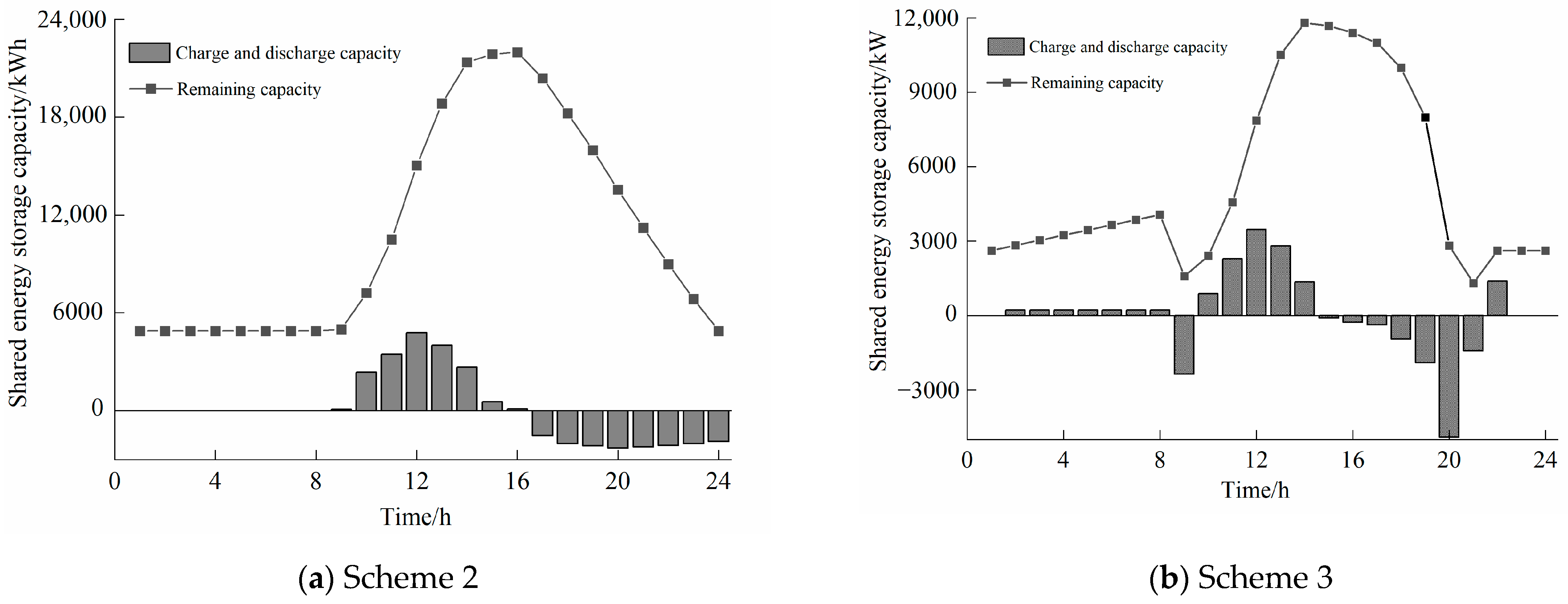
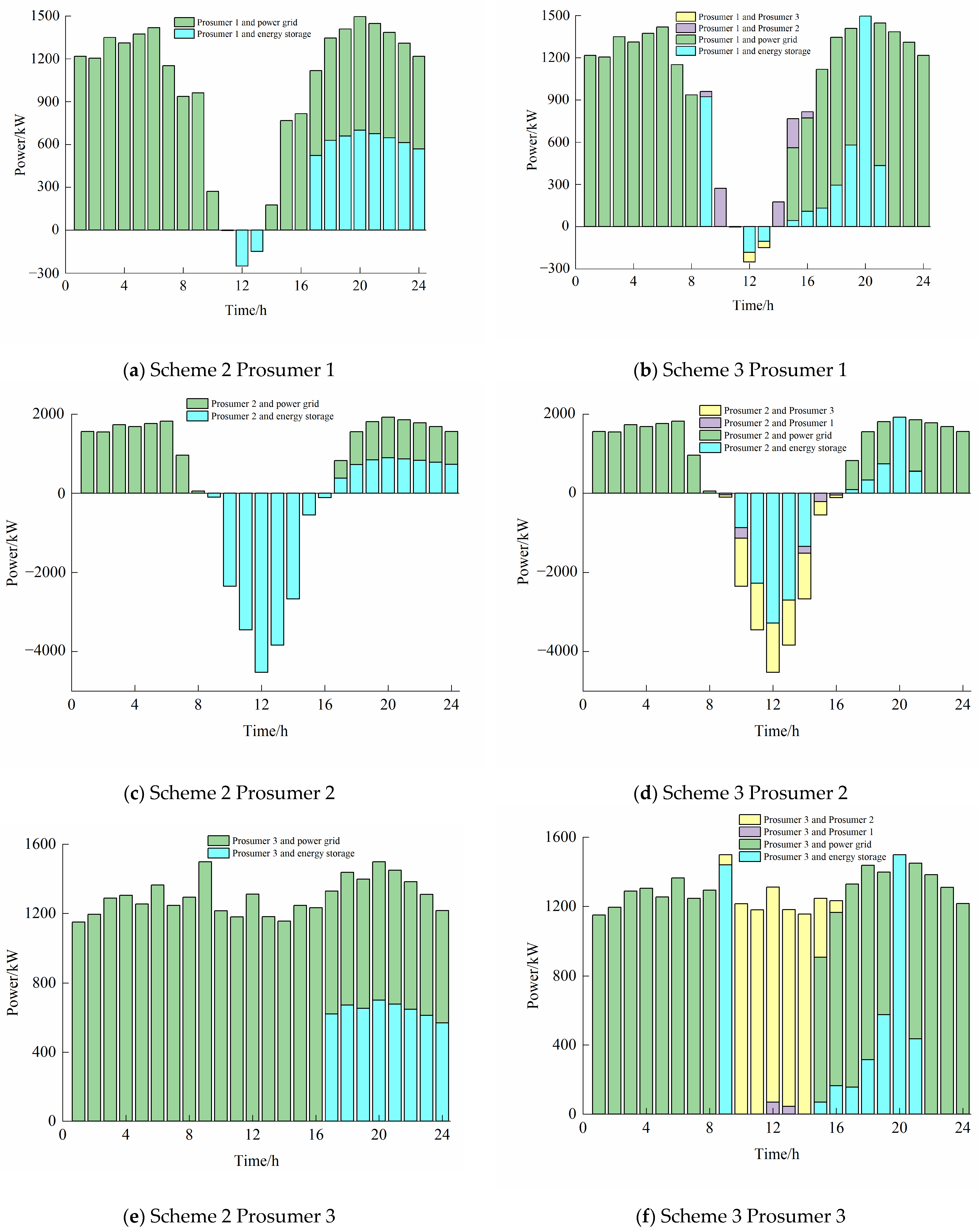
6.4. Analysis of the Operation Optimization Results of SES and Prosumers

The operation optimization results of the SES and prosumers are shown in Figure 3 and Figure 4. In Scheme 2, from 9:00 to 16:00, the power generation of Prosumer 1 and Prosumer 2 is greater than their power consumption. The prosumers sell the surplus power to the SES, and the remaining power of the SES reaches its peak at 16:00. From 17:00 to 24:00, the power generation of all prosumers is less than their power consumption. The SES sells power to the prosumers. In all time periods, when the power supply from PV power generation and energy storage is insufficient, the prosumers purchase power from the grid to meet their power demands. In Scheme 3, from 0:00 to 8:00, PV power generation is very low, and the grid electricity price is in the valley period. The prosumers purchase the insufficient power from the grid, while the SES purchases power from the grid to prepare for selling it at peak prices to earn profits. From 10:00 to 15:00, it is the high-generation period of PV power. The PV power generated by Prosumer 2 is first sold to Prosumer 1 and Prosumer 3 after meeting his or her own demand. The remaining power is then sold to the SES. The remaining power of the SES reaches its peak at 14:00. Meanwhile, Prosumer 1 also sells a small amount of power to Prosumer 3. The above-mentioned behaviors reduce the prosumers′ demand for energy storage and increases the autonomy of their power transactions. At 9:00 and 16:00 to 21:00, it is the low-generation period of PV power, and the grid electricity price is in the peak and flat periods. The prosumers prefer to purchase the insufficient power from the SES to reduce their electricity costs. The SES, based on the principle of maximizing profits, sells most of its power at the peak selling price of energy storage to increase its revenue. From 22:00 to 24:00, the remaining power of the SES is close to the lower limit of the state of charge, and the grid electricity price is in the flat period. Therefore, the prosumers purchase power from the grid to meet their own demands. The SES purchases some power from the grid to ensure the initial power state for the next day.

The above analysis indicates that, compared with traditional SES, the multi-prosumer energy complementation bilevel optimization model based on SES proposed in this paper can fully leverage the complementary advantages among prosumers, effectively reduce the electricity costs of prosumers and the capacity configuration of SES, achieve a win–win situation for prosumers and SES, and the PV consumption rate reaches 100%.

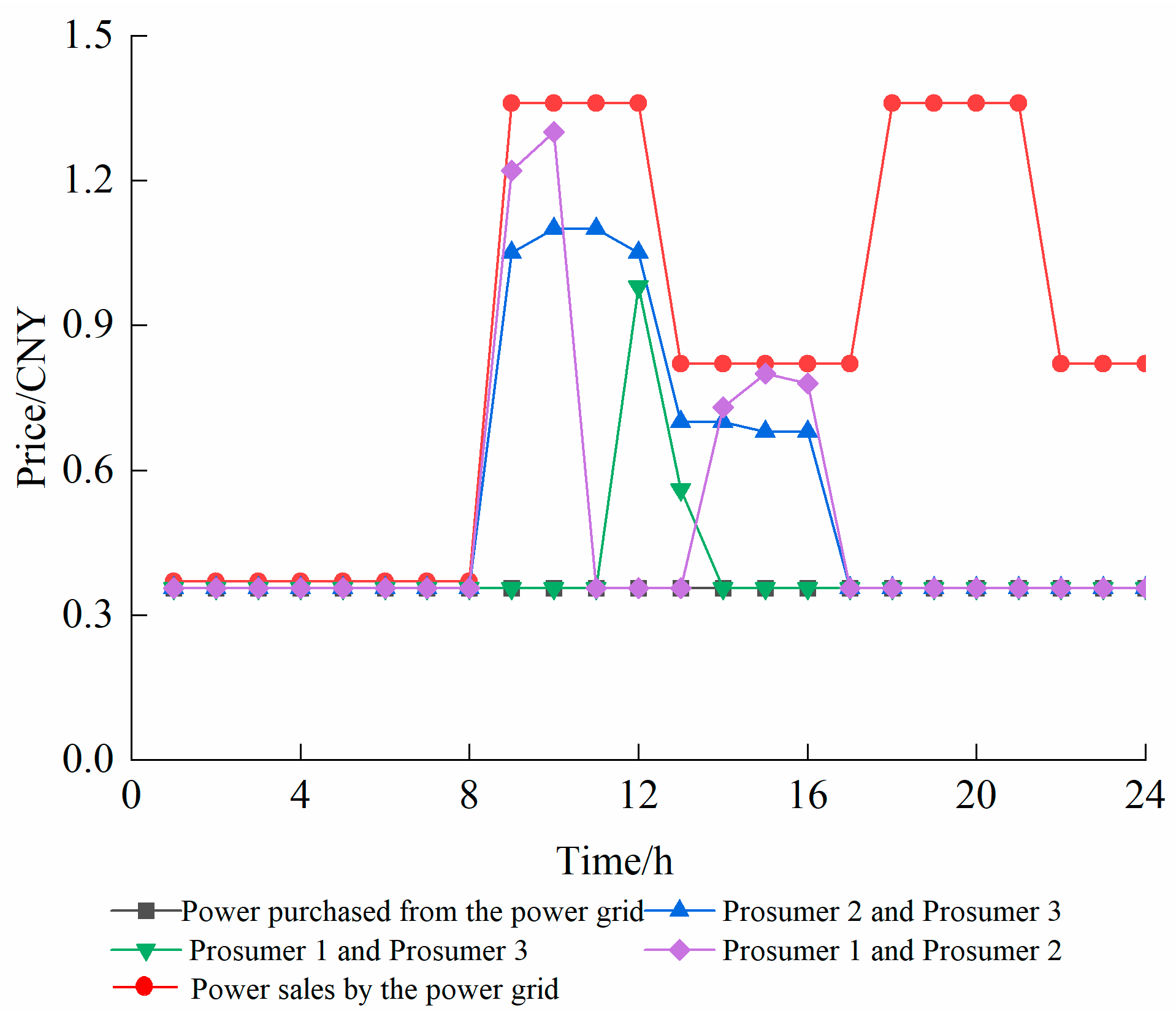
6.5. Analysis of the Transaction Results Between Prosumers

Based on the above optimal operation plan for prosumers, the purchase and sale electricity volumes of each prosumer participating in P2P transactions are shown in

Table 5. P2P transaction electricity purchase volume and electricity sale volume.

	Electricity Purchase Volume/kWh	Electricity Sell Volume/kWh
Prosumer 1	736.5	113.5
Prosumer 2	0	7130.6
Prosumer 3	6507.6	0
Total	7244.1	7244.1

. By substituting the corresponding data into Equation (31), the bargaining factors of each prosumer can be obtained. Then, by substituting these bargaining factors into the objective function in Equation (32), the P2P transaction prices among prosumers can be optimized and derived, and subsequently, the profits of each prosumer can be calculated. The savings of each prosumer obtained using the improved Nash bargaining method proposed in this paper are shown in

Table 6. Prosumer savings benefits.

Trading Entity	Bargaining Factor	Savings/CNY
Prosumer 1	0.054	96
Prosumer 2	1.676	4077
Prosumer 3	0.535	1396

, and the transaction electricity prices among prosumers are shown in Figure 5. The analysis shows that the transactions among prosumers have led to varying degrees of revenue improvement for each prosumer, and the benefits have been reasonably distributed according to the contribution of each prosumer to the transaction process. Specifically, Prosumer 1 is a balanced prosumer, whose generated electricity is mainly used to meet his or her own demand, and the purchase and sale of electricity to other prosumers are relatively small, with a bargaining factor of only 0.054, and thus this prosumer gains less. Prosumer 2 is a power-surplus prosumer, providing most of the electricity in the transaction process, while Prosumer 3 is a power-deficient prosumer, receiving most of the electricity in the transaction process. Therefore, they have higher contributions to the transaction process and gain more. Taking Prosumer 1 and Prosumer 2 as examples to analyze the transaction electricity prices among prosumers, from 9:00 to 10:00 and from 13:00 to 15:00, Prosumer 2 has excess electricity generation, while Prosumer 1 has insufficient electricity generation. Prosumer 2 sells electricity to Prosumer 1 at a price higher than the grid′s purchase price, and for Prosumer 1, the purchase price from Prosumer 2 is lower than that from the grid. Therefore, both parties have achieved a revenue improvement.

7. Conclusions

This paper establishes a bilevel optimization model for multi-prosumer power complementarity based on SES for energy consumption systems with multiple different types of prosumers. The validity of the model is verified through a case study, and the following conclusions are drawn:

(1)

The bilevel optimization model for multi-prosumer power complementarity based on SES proposed in this paper can enhance the operational revenue of the energy storage station and reduce the electricity cost of prosumers by reasonably regulating the interaction between the energy storage station and prosumers, achieving a win–win situation for both.

(2)

The electricity trading among prosumers can leverage the complementarity of power generation and consumption among different types of prosumers. PV power generation is prioritized for internal trading among prosumers, reducing the demand for energy storage and significantly lowering the required capacity of energy storage.

(3)

The introduced improved Nash bargaining method can rationally allocate the benefits of P2P trading among prosumers based on their contributions to the trading process. Moreover, internal negotiation of pricing among prosumers enables them to set more favorable trading prices without being restricted by the grid and energy storage purchase and sale prices, thereby increasing the benefits of all prosumers.

Furthermore, this article has not yet taken into account issues such as the degradation of the energy storage system and the corresponding subsidy policies. In future research, factors such as the decay of the energy storage capacity and carbon trading income can be incorporated into the modeling process. This will enable the calculated results to be closer to the actual situation in the real world.

References

1. Xu, M.Y.; Yang, Y.B.; Xu, Q.S.; Fang, L.L.; Tang, R.C.; Ji, H.M. Asymmetric Nash bargaining for cooperative operation of shared energy storage with multi-type users engagement. Front. Energy Res. 2024, 12, 1420393. [Google Scholar] [CrossRef]
2. Pan, W.J.; Zhang, Y.; Jin, W.W.; Liang, Z.D.; Wang, M.N.; Li, Q.Q. Photovoltaic-Based Residential Direct-Current Microgrid and Its Comprehensive Performance Evaluation. Appl. Sci. 2023, 13, 12890. [Google Scholar] [CrossRef]
3. Yang, H.J.; Yang, Z.C.; Gong, M.C.; Tang, K.; Shen, Y.M.; Zhang, D.B. Commercial operation mode of shared energy storage system considering power transaction satisfaction of renewable energy power plants. J. Energy Storage 2025, 105, 114738. [Google Scholar] [CrossRef]
4. Cui, J.D.; Zhu, Z.C.; Qu, G.L.; Wang, Y.Q.; Li, R.T. Demand-side shared energy storage pricing strategy based on stackelberg-Nash game. Int. J. Electr. Power Energy Syst. 2025, 164, 110387. [Google Scholar] [CrossRef]
5. Kang, W.F.; Chen, M.Y.; Li, Q.; Lai, W.; Luo, Y.Y.; Tavner, P.J. Distributed Optimization Model and Algorithms for Virtual Energy Storage Systems Using Dynamic Price. J. Clean. Prod. 2020, 289, 125440. [Google Scholar] [CrossRef]
6. Vankudoth, L.; Badar, Q.A. Development and analysis of scheduling strategies for utilizing shared energy storage system in networked microgrids. J. Energy Storage 2024, 97, 112691. [Google Scholar] [CrossRef]
7. Deng, W.Y.; Xiao, D.L.; Chen, M.L.; Tahir, M.F.; Zhu, D.R. Multi-regional energy sharing approach for shared energy storage and local renewable energy resources considering efficiency optimization. Int. J. Electr. Power Energy Syst. 2025, 167, 110592. [Google Scholar] [CrossRef]
8. Wang, Z.C.; Chen, L.J.; Li, X.Z.; Mei, S.W. A Nash bargaining model for energy sharing between micro-energy grids and energy storage. Energy 2023, 283, 129065. [Google Scholar] [CrossRef]
9. Sun, L.L.; Qiu, J.; Han, X.; Dong, Z.Y. Energy sharing platform based on call auction method with the maximum transaction volume. Energy 2021, 225, 120237. [Google Scholar] [CrossRef]
10. Qiao, J.P.; Mi, Y.; Shen, J.; Lu, C.K.; Cai, P.C.; Ma, S.Y.; Wang, P. Optimization schedule strategy of active distribution network based on microgrid group and shared energy storage. Appl. Energy 2025, 377, 124681. [Google Scholar] [CrossRef]
11. Wang, Y.X.; Chen, J.J.; Zhao, Y.L.; Xu, B.Y. Incorporate robust optimization and demand defense for optimal planning of shared rental energy storage in multi-user industrial park. Energy 2024, 301, 131721. [Google Scholar] [CrossRef]
12. Li, Y.; Qian, F.Y.; Gao, W.J.; Fukuda, H.; Wang, Y.F. Techno-economic performance of battery energy storage system in an energy sharing community. J. Energy Storage 2022, 50, 104247. [Google Scholar] [CrossRef]
13. Awnalisa, W.; Soongeol, K. Analysis on impact of shared energy storage in residential community: Individual versus shared energy storage. Appl. Energy 2021, 282, 116172. [Google Scholar]
14. Zhang, W.Y.; Zheng, B.S.; Wei, W.; Chen, L.J.; Mei, S.W. Peer-to-peer transactive mechanism for residential shared energy storage. Energy 2022, 246, 123204. [Google Scholar] [CrossRef]
15. Barkouki, B.E.; Laamim, M.; Rochd, A.; Chang, J.W.; Benazzouz, A.; Ouassaid, M.; Jeong, H. An Economic Dispatch for a Shared Energy Storage System Using MILP Optimization: A Case Study of a Moroccan Microgrid. Energies 2023, 16, 4601. [Google Scholar] [CrossRef]
16. Xie, Y.Z.; Yao, Y.; Wang, Y.W.; Cha, W.Q.; Zhou, S.; Wu, Y.; Huang, C.Y. A Cooperative Game-Based Sizing and Configuration of Community-Shared Energy Storage. Energies 2022, 15, 8626. [Google Scholar] [CrossRef]
17. Yang, Y.L.; Chen, T.; Yan, H.; Wang, J.Q.; Yan, Z.W.; Liu, W.Y. Optimization Operation Strategy for Shared Energy Storage and Regional Integrated Energy Systems Based on Multi-Level Game. Energies 2024, 17, 1770. [Google Scholar] [CrossRef]
18. Zhang, B.Q.; Huang, J.W. Shared Energy Storage Capacity Configuration of a Distribution Network System with Multiple Microgrids Based on a Stackelberg Game. Energies 2024, 17, 3104. [Google Scholar] [CrossRef]
19. Li, C.P.; Liu, Y.; Li, J.H.; Liu, H.J.; Zhao, Z.Q.; Zhou, H.G.; Li, Z.; Zhu, X.X. Research on the optimal configuration method of shared energy storage basing on cooperative game in wind farms. Energy Rep. 2024, 12, 3700–3710. [Google Scholar] [CrossRef]
20. Wang, Z.C.; Chen, L.J.; Li, X.Z.; Mei, S.W. A two-stage optimization approach-based energy storage sharing strategy selection for limited rational users. J. Energy Storage 2024, 93, 112098. [Google Scholar] [CrossRef]
21. Li, B.Y.; Yang, Q.M.; Kamwa, I. A Novel Stackelberg-Game-Based Energy Storage Sharing Scheme Under Demand Charge. IEEE/CAA J. Autom. Sin. 2023, 10, 462–473. [Google Scholar] [CrossRef]
22. Xie, Y.L.; Li, L.; Hou, T.Y.; Luo, K.; Xu, Z.Y.; Dai, M.C.; Zhang, L.X. Shared energy storage configuration in distribution networks: A multi-agent tri-level programming approach. Appl. Energy 2024, 372, 123771. [Google Scholar] [CrossRef]
23. Yang, M.; Zhang, Y.H.; Liu, J.H.; Yin, S.; Chen, X.; She, L.H.; Liu, H.M. Distributed Shared Energy Storage Double-Layer Optimal Configuration for Source-Grid Co-Optimization. Processes 2023, 11, 2194. [Google Scholar] [CrossRef]
24. Du, X.L.; Li, X.Z.; Hao, Y.B.; Chen, L.J. Sizing of centralized shared energy storage for resilience microgrids with controllable load: A bi-level optimization approach. Front. Energy Res. 2022, 10, 954833. [Google Scholar] [CrossRef]
25. Fernandez, E.; Hossain, M.J.; Mahmud, K.; Nizami, M.; Kashif, M. A Bi-level optimization-based community energy management system for optimal energy sharing and trading among peers. J. Clean. Prod. 2021, 279, 123254. [Google Scholar] [CrossRef]
26. Li, Q.Q.; Pan, W.J.; Jin, W.W.; Li, Q.; Liang, Z.D.; Li, Y. A new method to improve the power quality of photovoltaic power generation based on 24 solar terms. Sci. Rep. 2025, 15, 14406. [Google Scholar] [CrossRef] [PubMed]
27. Rodrigues, D.L.; Ye, X.M.; Xia, X.H.; Zhu, B. Battery energy storage sizing optimisation for different ownership structures in a peer-to-peer energy sharing community. Appl. Energy 2020, 262, 114498. [Google Scholar] [CrossRef]
28. Fausto, A.C.; Patryk, S.; Egidijus, K.; Erik, J.; Irina, T.; Jakub, J. Temporal dynamics and extreme events in solar, wind, and wave energy complementarity: Insights from the Polish Exclusive Economic Zone. Energy 2024, 305, 132268. [Google Scholar]
29. Jakub, J.; Paweł, T.; Bogdan, B.; Alban, K.; Egidijus, K.; Diyi, C.; Bo, M. Solar-hydro cable pooling—Utilizing the untapped potential of existing grid infrastructure. Energy Convers. Manag. 2024, 306, 118307. [Google Scholar]
30. Shahzad, J.M.; Jurasz, J.; Ruggles, T.H.; Khan, I.; Ma, T. Designing off-grid renewable energy systems for reliable and resilient operation under stochastic power supply outages. Energy Convers. Manag. 2023, 294, 117605. [Google Scholar] [CrossRef]
31. Cao, S.M.; Zhang, H.L.; Cao, K.; Chen, M.; Wu, Y.; Zhou, S.Y. Day-Ahead Economic Optimal Dispatch of Microgrid Cluster Considering Shared Energy Storage System and P2P Transaction. Front. Energy Res. 2021, 9, 645017. [Google Scholar] [CrossRef]
32. Duan, P.F.; Zhao, B.X.; Zhang, X.H.; Fen, M.D. A day-ahead optimal operation strategy for integrated energy systems in multi-public buildings based on cooperative game. Energy 2023, 275, 127395. [Google Scholar] [CrossRef]
33. Takayama, S.; Ishigame, A. A Voltage-Aware P2P Power Trading System Aimed at Eliminating Unfairness Due to the Interconnection Location. Energies 2024, 17, 841. [Google Scholar] [CrossRef]
34. Yan, M.Y.; Shahidehpour, M.; Paaso, A.; Zhang, L.X.; Alabdulwahab, A.; Abusorrah, A. Distribution Network-Constrained Optimization of Peer-to-Peer Transactive Energy Trading Among Multi-Microgrids. IEEE Trans. Smart Grid 2021, 12, 1033–1047. [Google Scholar] [CrossRef]
35. Zhao, W.H.; Xu, S.T.; Guo, P. Optimization Decision Study of Business Smart Building Clusters Considering Shared Energy Storage. Sustainability 2024, 16, 3422. [Google Scholar] [CrossRef]
36. Chen, Y.; He, S.; Wang, W.Q.; Yuan, Z.; Cheng, J.; Cheng, Z.J.; Fan, X.C. Optimization Strategy for Shared Energy Storage Operators-Multiple Microgrids with Hybrid Game-Theoretic Energy Trading. Processes 2024, 12, 218. [Google Scholar] [CrossRef]
37. Jung, S.P.; Seung, W.K.; Ji, W.L. P2P credit auction vs. net metering: Benefit analysis for prosumers under incremental block rate electricity tariff. Appl. Energy 2024, 364, 123095. [Google Scholar]
38. Manchalwar, A.D.; Patne, N.R.; Pemmada, S.; Panigrahi, R.; Morey, C. Decentralized peer-to-peer model of energy trading in smart grid considering price differentiation. Energy Rep. 2023, 9 (Suppl. S10), 728–736. [Google Scholar] [CrossRef]
39. Mohammad, H.G.; Hossein, Y.; Behnam, M.I. An internal pricing method for a local energy market with P2P energy trading. Energy Strategy Rev. 2025, 58, 101673. [Google Scholar]
40. Noorfatima, N.; Choi, Y.; Jung, J. Two-stage peer-to-peer energy trading with combined uniform and discriminatory pricing mechanism. Renew. Energy 2025, 247, 123014. [Google Scholar] [CrossRef]
41. Wang, G.Y.; Wang, C.F.; Niu, Y.F.; Yao, W.L.; Wang, K. Cooperative Optimal Decision-making for Active Distribution Network with Shared Energy Storage Leased by Prosumers. Power Syst. Autom 2025, 49, 105–116. [Google Scholar]
42. Yu, J.W.; Bao, S.Y.; Li, S.; Wu, H.L.; Li, H.X. Robust Optimization of Multi-Microgrid Systems in CCHP Regions Considering Self-Built Shared Energy Storage Station. Acta Energiae Solaris Sin. 2025, 46, 503–513. [Google Scholar]
43. Wu, S.J.; Li, Q.; Liu, J.K.; Zhou, Q.; Wang, C.G. Bi-level Optimal Configuration for Combined Cooling Heating and Power Multi-microgrids Based on Energy Storage Station Service. Power Syst. Technol. 2021, 45, 3822–3832. [Google Scholar]
44. Ji, R.Q.; Hu, J.; Zhang, X.J.; Wang, L.; Yang, Z.J. Cost Optimization of Shared Energy Storage in Building Cluster Based on Service of a Third-party Agent. High Volt. Eng. 2024, 50, 2523–2536. [Google Scholar]
Figure 1. System structure diagram.
Sustainability 17 05890 g001
Figure 2. Flowchart of the solution method.
Sustainability 17 05890 g002
Figure 3. Operation optimization results of SES.
Sustainability 17 05890 g003
Figure 4. Optimization results of prosumer operation.
Sustainability 17 05890 g004
Figure 5. Transaction electricity prices between prosumers.
Sustainability 17 05890 g005