Abstract
Parks play a crucial role in mitigating urban heat island effects, a key challenge for urban sustainability. Park cooling intensity (PCI) mechanisms across varying canopy-layer urban heat island (CUHI) gradients remain underexplored, particularly regarding interactions with meteorological, topographical, and socio-economic factors. According to the urban-suburban air temperature difference, this study classified the city into non-, weak, and strong CUHI regions. We integrated causal inference, machine learning and a geographical detector (Geodetector) to model and interpret PCI dynamics across CUHI gradients. The results reveal that surrounding impervious surface coverage is a universal driver of PCI by enhancing thermal contrast at park boundaries. However, the dominant drivers of PCI varied significantly across CUHI gradients. In non-CUHI regions, surrounding imperviousness dominated PCI and exhibited bilaterally enhanced interaction with intra-park patch density. Weak CUHI regions relied on intra-park green coverage with nonlinear synergies between water body proportion and park area. Strong CUHI regions involved systemic urban fabric influences mediated by surrounding imperviousness, evidenced by a validated causal network. Crucially, causal inference reduces model complexity by decreasing predictor counts by 79%, 25% and 71% in non-, weak and strong CUHI regions, respectively, while maintaining comparable accuracy to full-factor models. This outcome demonstrates the efficacy of causal inference in eliminating collinear metrics and spurious correlations from traditional feature selection, ensuring retained predictors reside within causal pathways and support process-based interpretability. Our study highlights the need for context-adaptive cooling strategies and underscores the value of integrating causal–statistical approaches. This framework provides actionable insights for designing climate-resilient blue–green spaces, advancing urban sustainability goals. Future research should prioritize translating causal diagnostics into scalable strategies for sustainable urban planning.
1. Introduction
In urban environments, blue–green spaces that combine water bodies and vegetation coverage can provide cooling through evaporation and shading to mitigate urban heat island (UHI) effects [1,2,3,4]. Parks, as important components of the blue–green infrastructure in urban ecosystems, play a crucial role in regulating urban temperatures and improving microclimate conditions [5,6]. Many studies have been carried out to understand how urban landscape configurations influence the park cooling effect, which is pivotal for guiding the design of urban spaces to enhance the well-being of urban residents.
Park cooling intensity (PCI) is a key metric for evaluating the thermal regulation capacity of a park which quantifies the thermal gradient from park interiors to surrounding areas [7,8,9,10,11]. It is well-documented that PCI is influenced by internal factors such as park area, boundary shape, vegetation coverage, and presence of water bodies. Additionally, PCI is significantly affected by the configuration of land cover features outside the park [12,13,14], especially the spatial distribution of artificial impervious surfaces [15,16,17].
Studies on the role of land cover composition and landscape patterns as determinants of the park cooling effect are exhaustive [18,19,20,21]. This body of work largely employs remote sensing techniques to acquire the land surface temperature (LST) distribution and urban land cover classification, which subsequently facilitates quantification of the park cooling effect and the identification of related landscape factors [22,23]. Methods including multiple linear regression [15,24,25,26], geographically weighted regression (GWR) [27,28], machine learning with SHapley Additive exPlanations (SHAP) [29], and geographical detectors (Geodetector) [20,30,31] are employed to analyze associations between PCI and urban landscapes, with emphasis on identifying key explanatory factors and their interactions.
Previous research on urban thermal environments has extensively focused on the surface urban heat island (SUHI) effect. Remote sensing imagery can provide detailed spatial insights into LST variations [32,33,34]. However, investigations into the mechanisms underlying the relationship between SUHI and the Canopy-layer urban heat island (CUHI) effect, which pertains to near-surface air temperature, remain relatively limited [35,36]. This knowledge gap extends to the mechanisms driving park cooling effects across varying CUHI gradients, shaped by distinct landscape and socio-economic drivers.
A further limitation of the existing research is its predominant focus on urban landscape impacts, often neglecting other potentially influential factors such as meteorological conditions, topographical features, and socio-economic aspects [37,38,39,40]. This narrow scope risks overlooking the multifaceted nature of the complex interactions between the park cooling effect and urban thermal environment. Furthermore, statistical methods for modeling PCI with its potential influential factors often rely on correlation analysis while neglecting causal relationships. This neglect of causality represents a critical limitation, particularly as causal inference is essential for uncovering causal links and distinguishing them from spurious correlations [41,42,43,44,45]. Causal inference analysis can be used to identify and retain variables that make a substantial contribution to the predictive power of the model, while removing irrelevant or redundant variables [46,47]. Through such feature selection by causal inference analysis [48], the model’s interpretability can be improved because a model with fewer, causally relevant variables is generally more transparent and explainable.
This identified research gap holds significant implications for urban planning. CUHI gradients correspond to distinct urban morphologies (e.g., urban core–periphery structures), necessitating context-specific cooling strategies. However, systematic investigations into PCI mechanism variations across CUHI gradients remain lacking. Moreover, the integration of causal inference into PCI studies to resolve feature collinearity, a critical barrier to generating actionable insights, remains unexplored. To address these gaps, this study investigates how multifactorial drivers influence PCI across stratified CUHI gradients. We expand the analytical scope beyond landscape factors by incorporating meteorological, topographical, and socio-economic variables. GWR was employed to account for the spatial heterogeneity of these influential factors. Causal inference analysis identified relationships between the potential influential factors and PCI within each CUHI gradient. PCI was modeled using a machine learning algorithm. Crucially, PCI models incorporating all potential influential factors were compared with those refined through causal inference and SHAP importance ranking to evaluate the effectiveness of causal inference for feature selection. The importance of the individual factors and their interactions in the PCI models was evaluated and compared among different CUHI gradients, aiming to achieve a comprehensive understanding of the park cooling mechanisms inherent to UHI phenomena. By decoding gradient-specific cooling mechanisms, this study provides evidence-based pathways to enhance urban thermal resilience through targeted blue–green infrastructure planning.
2. Materials and Methods
2.1. Study Area
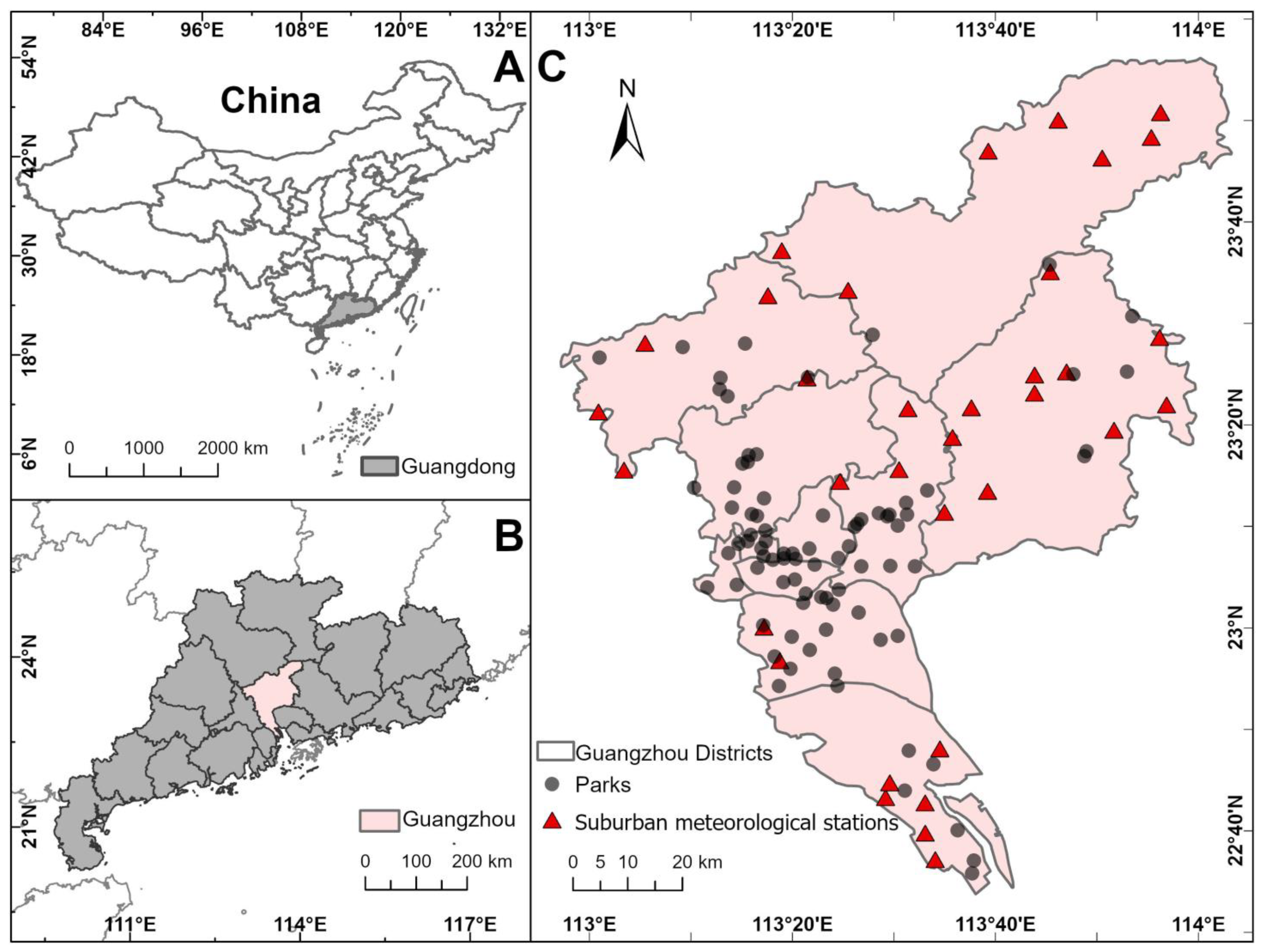
We investigated parks in Guangzhou, the capital city of Guangdong Province in China (Figure 1). Guangzhou is in the northern fringe of the Pearl River Delta (112°57′–114°3′ E, 22°26′–23°56′ N), dominated by a marine subtropical monsoon climate with an annual average temperature of 21–24 °C and an average relative humidity of 73%. As of 2022, Guangzhou has reached a permanent population of 18.73 million people (http://tjj.gz.gov.cn/ (accessed on 13 June 2025)). Concurrently, the ratio of the urban permanent population to the total urban population has reached 86.48%, reflecting accelerated urbanization and significant population concentration effects. Despite this substantial demographic expansion, Guangzhou has made commendable strides in the realm of green infrastructure development. In 2022, the urban green space coverage extended to 158,649 ha, with an impressive green space ratio of 44.2% in urban construction zones. The total number of parks increased to 530, covering an area of 76,678 ha. Although the green coverage area has increased over the past few years, complex impacts of urban expansion still lead to an increasingly severe urban heat island effect. The mere increment in green spaces is insufficient to counterbalance the impact of urban expansion and other factors on the urban thermal environment. Therefore, it is urgent to explore the formation mechanism of heat islands and optimize urban cooling strategies.

Figure 1.
Study area and park locations. (A) This study was conducted in Guangzhou, China. (B) Guangzhou is the capital city of Guangdong Province, dominated by a marine subtropical monsoon climate. (C) The suburban air temperature is determined by the average air temperature of the 34 suburban meteorological stations. There were 84 parks included in analysis for the years from 2014 to 2022.
For this study, we used data from 84 parks for the period spanning from 2014 to 2022 (Figure 1C). We selected parks with an area greater than 10 ha to ensure a diverse landscape spatial configuration of the park and its surroundings. The park areas ranged from 10.19 to 925.45 ha, with park perimeters varying from 1.39 to 23.83 km. The parks are primarily located in the central part of Guangzhou; those farther from the city center tend to be larger in area.
We located suburban representative stations for CUHI gradient classification according to the Guangzhou Urban Heat Island Monitoring Bulletin 2023 issued by the Guangzhou Climate and Agricultural Meteorological Center (http://www.tqyb.com.cn/gz/climaticprediction/bulletin/ (accessed on 13 June 2025)). Meteorological stations were categorized into three groups, including suburban stations, urban stations and high-altitude stations. From the suburban and urban groups, 12 urban representative stations and 34 suburban representative stations (Figure 1C) were selected through a comprehensive evaluation of spatial and socio-economic indicators, including land use type classification, elevation, terrain characteristics, population density, gross domestic product, and nighttime light index. This multi-criteria framework ensured the systematic identification of stations reflecting distinct urban and suburban climatic profiles while minimizing anthropogenic interference.
2.2. Data Collection
The shapefiles of the parks that specified the park locations and shapes were obtained from OpenStreetMap (https://download.geofabrik.de/asia/china.html, (accessed on 13 June 2025), see Table 1). Landsat Collection 2 data for calculation of the spectral indices quantifying land cover properties were obtained from the United States Geological Survey (USGS, https://www.usgs.gov/landsat-missions (accessed on 13 June 2025)). Due to the abundant rainfall in Guangzhou for most of the year, the imaging quality of the Landsat 8 satellite is often affected by cloud cover, especially during the summer when it is difficult to obtain cloud-free satellite images. This study calculated the maximum values of LST for each summer season (from mid-May to mid-October) between 2014 and 2022 using the Google Earth Engine (GEE, https://code.earthengine.google.com (accessed on 13 June 2025)). The LST imagery data were used to quantify the PCI values. The land cover classification imagery for calculation of the landscape metrics quantifying the landscape configurations were obtained from China Land Cover Datasets (CLCD, https://zenodo.org/records/8176941 (accessed on 13 June 2025)). Given the main land cover types in Guangzhou, we reclassified the land cover types of CLCD into five categories, including crop land, green space, water body, impervious surface and bare soil. The elevation data were obtained from the Advanced Spaceborne Thermal Emission and Reflection Radiometer Global Digital Elevation Model (ASTER GDEM) through the Geospatial Data Cloud platform (http://www.gscloud.cn (accessed on 13 June 2025)). The road shapefiles for calculation of road density were obtained from OpenStreetMap. The population data were obtained from LandScan (https://landscan.ornl.gov/citations (accessed on 13 June 2025)). The meteorological data, including rainfall and air temperature, were obtained from the National Tibetan Plateau Data Center (http://data.tpdc.ac.cn (accessed on 13 June 2025)).

Table 1.
Research data specification.
2.3. Data Analysis
2.3.1. Quantification of PCI
PCI was quantified by the difference in LST between the park and its cooling buffer zone:
where is the average LST of the park cooling buffer zone, excluding water bodies outside the park; is the average LST of the area inside the park. The park cooling buffer zone is designated using the equal-radius method [10,15]. The radius of the cooling buffer zone is equal to the radius of a circle with an area identical to that of the park:
where is the radius of the park cooling buffer zone; is the area of the park. The equal-radius method converts irregularly shaped parks into circular areas of equivalent size, ensuring standardized spatial analysis while accounting for park-scale variability. This simplification aligns with common practices in thermal environmental studies, which is relatively fast and effective especially for quantifying PCI compared to the fixed-radius method, the equal-area method and the inflection-point method [11,49].
2.3.2. Calculation of PCI Potential Influential Factor
We categorized the potential influential factors affecting PCI into four groups, including topographic factors, socio-economic factors, meteorological factors, and land cover factors (Table 2). The topographic factors include elevation and slope. The socio-economic factors include population density and road density. The meteorological factors include rainfall and air temperature. The land cover factors include a collection of spectral indices and landscape metrics. The landscape metrics were calculated using Fragstats (version 4.2).
Table 2.
Potential influential factors of PCI.
The potential influential factors () were geographically weighted by multiplying a spatial weight matrix ():
where represents the geographically weighted potential influential factors. was calculated from a Gaussian distance decay function [50]:
where is a non-negative bandwidth, determined by the minimum Akaike Information Criterion. represents the Euclidean Distance between park and park ; the weight value decays with the increase in distance [51].
2.3.3. Categorization of CUHI
We used the air temperature difference between the central urban areas and the suburbs to assess the urban heat island phenomenon. The suburban station locations were obtained from the Guangzhou Urban Heat Island Monitoring Bulletin 2023 issued by the Guangzhou Climate and Agricultural Meteorological Center (http://www.tqyb.com.cn/gz/climaticprediction/bulletin/ (accessed on 13 June 2025)), which provides 34 representative suburban meteorological stations in Guangzhou (Figure 1C. Using summer mean air temperature imagery from the National Tibetan Plateau Data Center, the average air temperature of these 34 suburban stations was calculated to determine the suburban background air temperature (). CUHI of each pixel on the image was defined by the difference between the air temperature of the given pixel () in the air temperature imagery and the [35]:
According to the value of , the city was classified into areas of non-CUHI (CUHI ≤ 0 °C), weak CUHI (0 °C < CUHI ≤ 0.5 °C) and strong CUHI (CUHI > 0.5 °C). The 0.5 °C threshold demarcating weak and strong CUHI zones was empirically derived from the observed CUHI magnitude range (−1.63–0.92 °C). This approximately equal-interval classification enhances differentiation between thermally distinct zones and reflects region-specific thermal characteristics. PCI was modeled and evaluated for different CUHI gradients.
2.3.4. Causal Inference Analysis
The causal relationships between PCI and potential influential factors were analyzed through a multi-step causal inference framework. The Peter–Clark (PC) causal discovery algorithm [43,52] was applied to all variables to construct an initial completed partial directed acyclic graph (CPDAG). In this CPDAG, directed edges represent established irreversible causal relationships, while undirected edges indicate uncertain causal directions, potentially reflecting latent dependencies. Subsequently, variables unrelated to PCI, defined as those exhibiting neither direct nor indirect causal paths to PCI, were systematically removed. The PC algorithm was then reapplied to the retained variables, with the existing directed edges from the initial CPDAG preserved to ensure consistency in known causal relationships. This step aimed to refine the causal structure by allowing the detection of new edges among the retained variables while maintaining the integrity of previously identified causal directions.
For unresolved undirected edges in the final CPDAG, the additive noise model (ANM) [53] was employed to infer causal directions by testing the independence between variables and residual noise. The structural equation model (SEM) [45] was integrated to further validate the causal model. The edges with p-values greater than 0.05 were discarded, yielding a deterministic directed causal network, i.e., a directed acyclic graph (DAG). The PC algorithm and ANM were implemented using the Causal-Learn Python library (version 0.1.3.8) (https://causal-learn.readthedocs.io/en/latest/ (accessed on 13 June 2025)) [54]. SEM was implemented using the Semopy Python library (version 2.3.11) (https://pypi.org/project/semopy/ (accessed on 13 June 2025)).
2.3.5. PCI Modeling and Assessment
The relationships between PCI and the potential influential factors within different CUHI gradients were modeled using CatBoost, a gradient boosting decision tree variant that employs ordered boosting and advanced categorical feature processing to mitigate prediction bias [55,56]. To account for inherent stochasticity in machine learning processes, we conducted 10 independent experimental trials with random data splits, where each trial maintained a 70% training and 30% testing allocation. The model performance was assessed using the averaged root mean square error (RMSE) and coefficient of determination (R2) across all trials, accompanied by their standard deviations to quantify result stability. The importance of the individual factors in the PCI model is assessed by SHAP [29], which is a machine learning model interpretation framework. SHAP determines the SHAP value for each feature by evaluating the prediction differences that arise from the presence or absence of that feature in all possible feature subsets, followed by averaging these differences with appropriate weighting [57,58]. CatBoost algorithm was implemented using the CatBoost Python library (version 1.2.3) through its scikit-learn compatible interface. SHAP analysis was implemented using the SHAP Python library (version 0.46).
Three modeling frameworks were systematically compared: (1) a full-factor model incorporating all potential variables, (2) a causal-factor model retaining variables selected through causal inference analysis to eliminate spurious correlations, and (3) a SHAP-optimized factor model matching the variable count of the causal-factor model but prioritizing features with the highest SHAP rankings. The causal inference approach ensured theoretical validity by preserving variables with causal linkages to PCI, whereas SHAP-based optimization enhanced predictive efficiency through data-driven feature prioritization.
The importance of the interactions among the influential factors in the PCI model was assessed by the interaction detector module of Geodetector, complementing the SHAP-based interpretation. The value is used to quantify the effect of the influential factor on the response variable in Geodetector [31,59]:
where = 1, 2, …, represents the stratification of variables; and stand respectively for the number of units in and the whole region. and stand respectively for the variance of units in and the global variance of the response variable over the whole region [60]. The interactive effect of two influential factors on the response variable is evaluated by comparing the values of the individual factors and their interaction (Table 3).
Table 3.
Types of interactions between two influential factors detected by Geodetector.
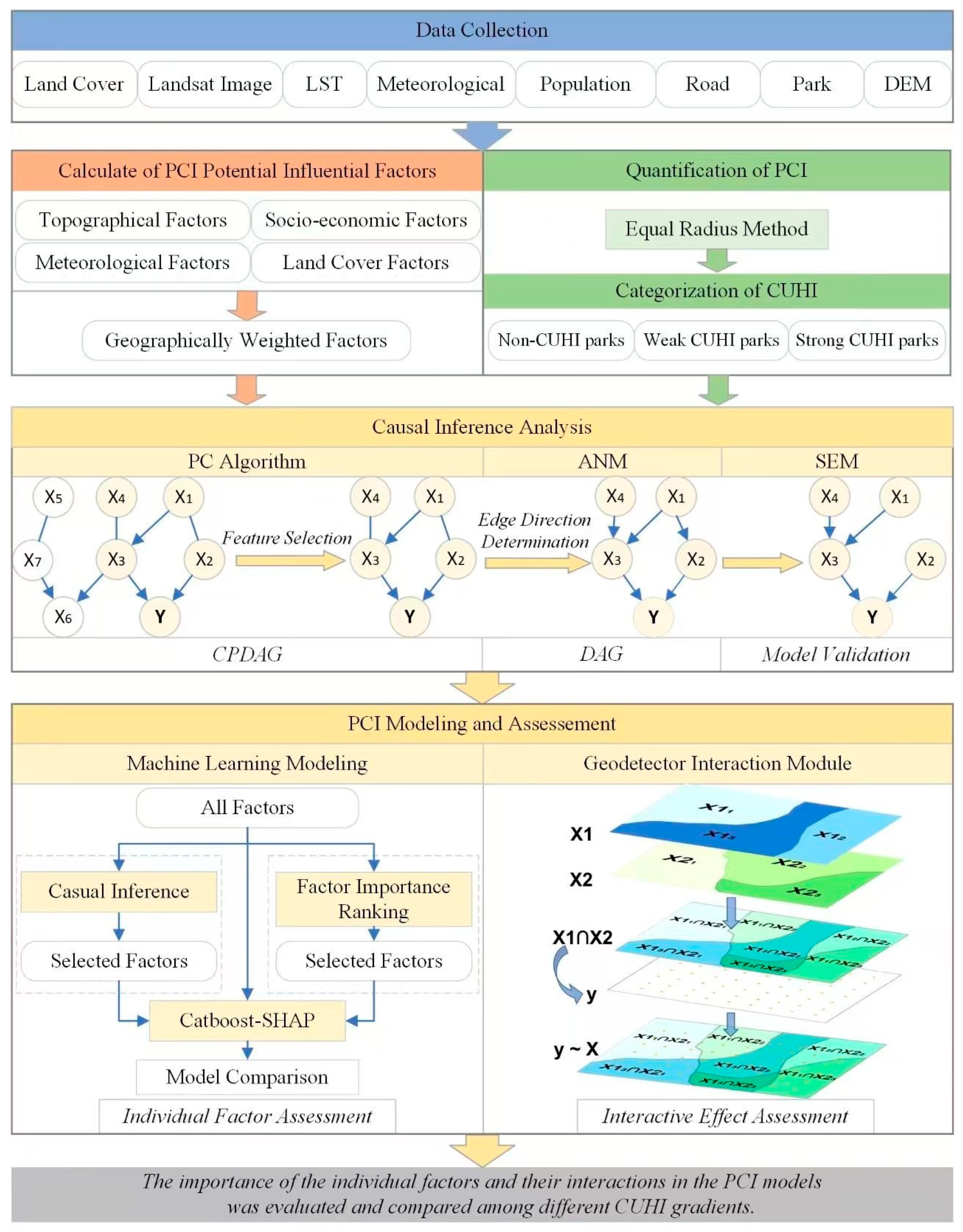
Through PCI modeling and influential factor assessment (Figure 2), our study aims to reveal significant insights into the determinants of PCI across varying gradients of CUHI in Guangzhou. The application of the PC algorithm for causal inference analysis is a pivotal step in feature selection, enabling a refined understanding of the causal pathways that underpin PCI. The comparative analysis of PCI models across varying CUHI gradients is designed to highlight the complexity of park cooling mechanisms and their intricate interactions with the urban thermal environment. Such an analysis is crucial for advancing our understanding of how parks mitigate urban heat, providing actionable insights for urban planning and environmental management strategies aimed at alleviating the UHI effect.
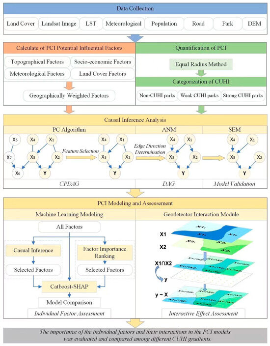
Figure 2.
Framework for analyzing of multifaced factors of PCI using a combination of causal inference analysis, geographically weighted machine learning and Geodetector.
3. Results
3.1. Interannual CUHI Gradient Variation
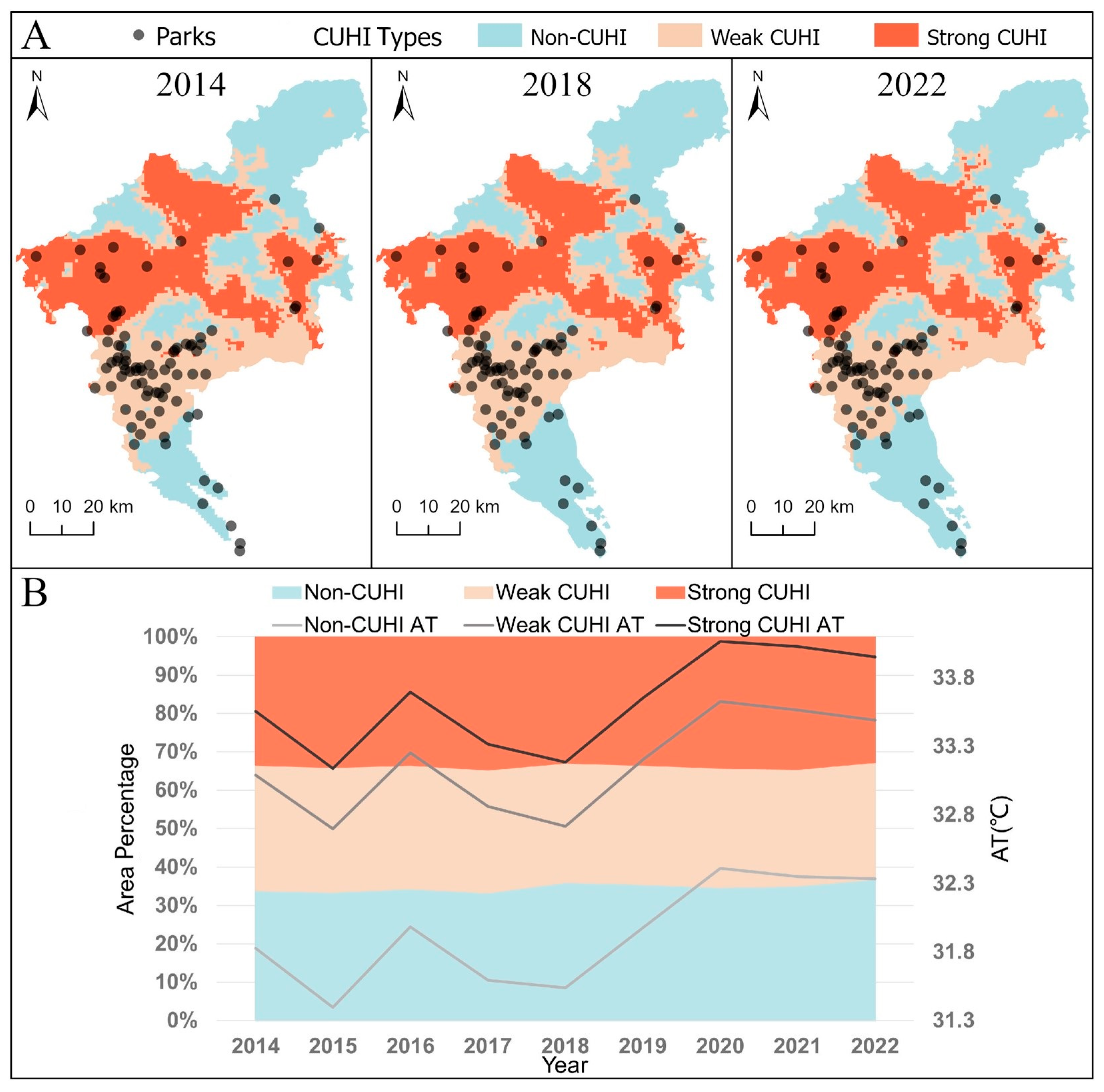
The distribution of CUHI gradients shows minimal variation across years (Figure 3). However, interannual fluctuations in air temperature are considerable, with an overall increasing trend. Parks in each CUHI gradient across years were gathered for modeling PCI, from which the key determinants that influence PCI across different levels of CUHI gradients were identified.
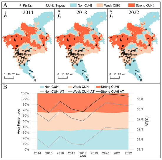
Figure 3.
Categorization of CUHI. (A) Parks in each CUHI gradient across years are gathered for modeling PCI. (B) The proportion distribution of different CUHI gradients is relatively consistent across years, whereas the variances in the average air temperature at different CUHI gradients across years are evident.
3.2. Gradient-Specific Causal Paths for PCI
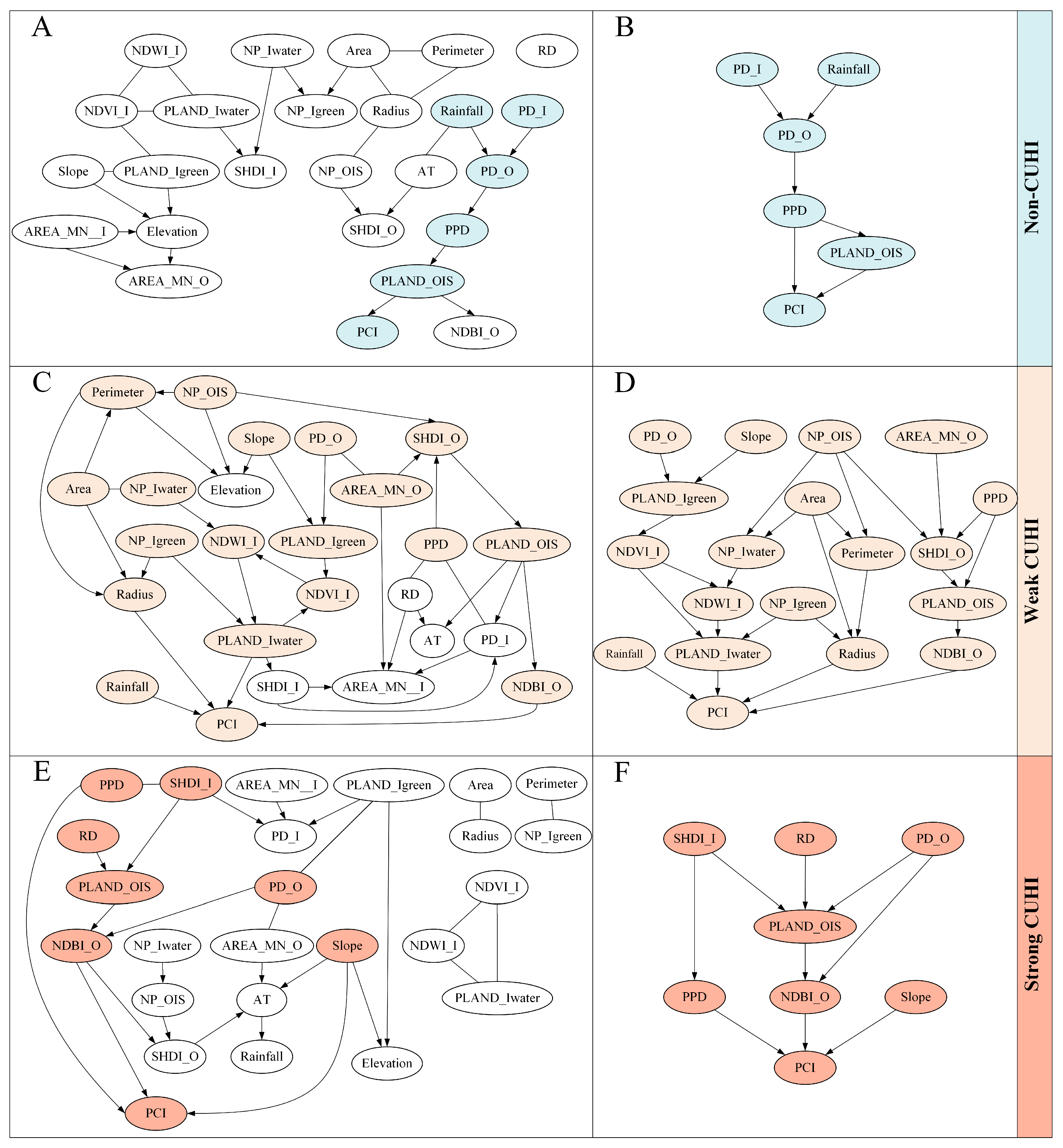
The PC algorithm facilitated the identification of causal relationships across all variables (Figure 4A,C,E). We extracted the direct and indirect causal factors related to PCI from the complete set of variables. These variables were then re-analyzed using the PC algorithm while maintaining the causal directionality in the original CPDAG, ultimately refining the causal inference models (Figure 4B,D,F). The resulting causal models were assessed by SEM analysis (Table 4).
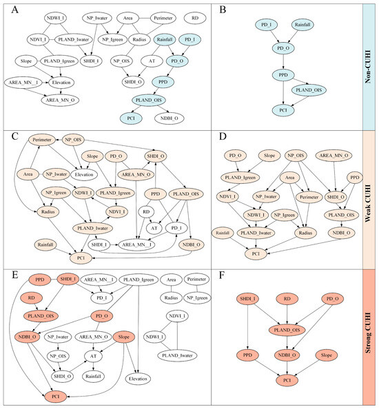
Figure 4.
Causal inference analyses of PCI and potential influential factors within the non-CUHI (A,B), the weak CUHI (C,D), and the strong CUHI (E,F). The PC algorithm was employed across all variables (A,C,E). The direct and indirect causal factors related to PCI were selected and re-analyzed to refine the causal inference models (B,D,F). The undirected edges were oriented using ANM, and their statistical significance was rigorously evaluated via SEM, yielding a DAG with definitive causal pathways.
Table 4.
Evaluation of the causal models by SEM. The optimal results are highlighted in bold.
The causal relationships between PCI and potential influential factors vary in different CUHI gradients. Within the non-CUHI gradient (Figure 4B), PPD and PLAND_OIS are the direct causes of PCI. PD_O is a direct cause of PPD, which is determined by PD_I and Rainfall.
Among the three CUHI gradients, the causal model for the weak CUHI gradient is the most complex, which incorporates the largest number of variables (Figure 4D). There are four direct causes of PCI, namely Rainfall, PLAND_Iwater, Radius and NDBI_O. Notably, PLAND_Iwater is constrained and influenced by multiple factors, include Slope, PD_O and NP_OIS, mediated through the structural and functional characteristics of the internal blue–green landscape configuration. Additionally, NDBI_O is indirectly modulated by PPD through associations mediated by SHDI_O and PLAND_OIS.
Within the strong CUHI gradient (Figure 4F), the direct causes of PCI include PPD, NDBI_O, and Slope. SHDI_I influences PCI indirectly through its mediation by PPD, establishing a secondary causal pathway. PLAND_OIS is jointly shaped by SHDI_I, RD, and PD_O, thereby mediating its effect on NDBI_O. Furthermore, PD_O exerts a direct causal influence on NDBI_O.
The evaluation of the causal models by SEM (Table 4) shows that the model for the strong-CUHI gradient has the best overall performance across multiple metrics, which validates causal inference for isolating dominant drivers of PCI in high-heat urban contexts. In contrast, the models for the non-CUHI and weak CUHI gradients exhibit critical misfit. Nevertheless, these underperforming models provide critical methodological and theoretical insights. Specifically, in non-CUHI regions, oversimplified models likely overlook key natural regulators. In weak CUHI systems, variable redundancy and collinear pathways obscure nonlinear cooling processes due to stochastic variability. These results highlight the necessity of context-specific modeling.
3.3. PCI Model Performance with Factor and Interaction Analysis
The comparative analysis of the three modeling approaches reveals context-dependent performance patterns across CUHI gradients (Table 5). For non-CUHI conditions, the full-factor model (24 factors) achieved superior accuracy, while the SHAP-optimized model (five factors) retained comparable predictive power, suggesting effective correlation-based feature compression. In contrast, the causal-factor model (five factors) exhibited significant performance decline, aligning with SEM misfit metrics that reveal oversimplification of natural regulatory mechanisms. Under weak CUHI conditions, while all three models exhibited minimal performance divergence, the causal model slightly outperformed the other two models. This parity implies substantial feature redundancy in the full-factor framework, as nearly 25% of factors could be eliminated without compromising predictive capability.
Table 5.
Performances of full-factor, causal-factor and SHAP-optimized factor models across different CUHI gradients.
For strong CUHI gradients, the full-factor model achieved marginally higher predictive accuracy compared to the causal-factor and SHAP-optimized factor models. The reduced-factor models demonstrate significant practical value by trimming the feature set by 71% (from 24 to seven factors) while maintaining comparable predictive capability. The advantage of the causal-factor model over the SHAP-optimized model aligns with SEM validation (Table 4), which confirms that the feature selection by causal inference preserves variables within statistically robust causal pathways. This distinction highlights the ability of causal inference to prioritize interpretable, theory-anchored drivers over the purely correlative feature rankings by SHAP analysis.
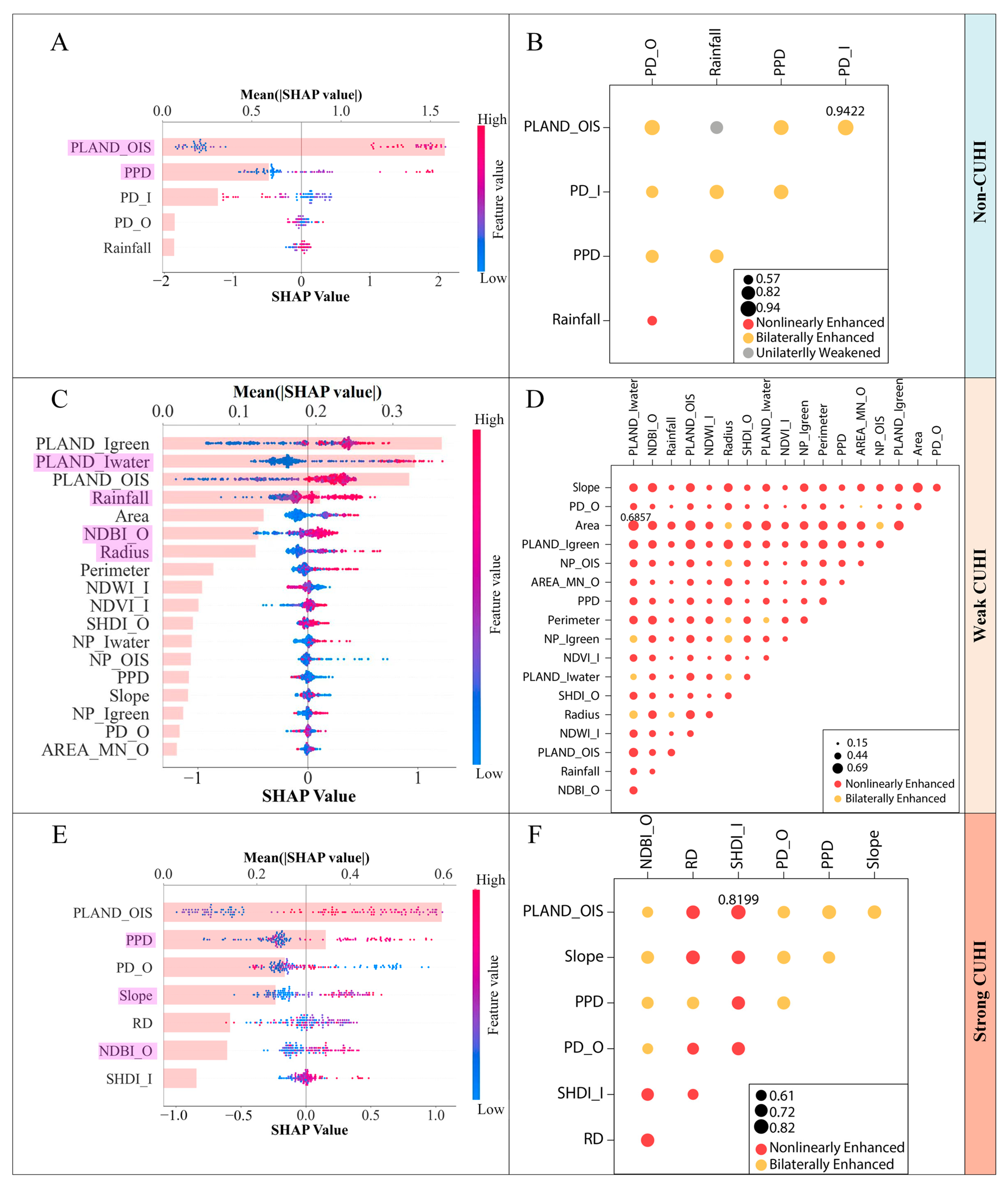
The importance of the factors in the models refined through causal inference was assessed by SHAP analysis (Figure 5A,C,E). Within the non-CUHI (Figure 5A) and strong CUHI (Figure 5E) gradients, PLAND_OIS is the most important factor in modeling PCI, which exhibits a significant positive association with PCI. PLAND_Igreen shows the strongest positive correlation with PCI in the weak CUHI gradient (Figure 5C). It was found that the direct causes of PCI identified in the causal inference may not necessarily rank highest in the SHAP analysis of factor importance.
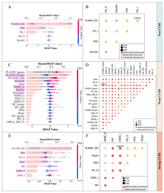
Figure 5.
The importance of the factors filtered by causal inference across different CUHI gradients. The importance of the individual factors was assessed by SHAP (A,C,E). The factors highlighted in light purple are the variables identified as the direct causes of PCI in the analysis of causal inference. The importance of the interactive effects between factors on PCI was assessed by the interaction module of Geodetector (B,D,F).
The importance of the interactive effects between factors on PCI was assessed by the interaction module of Geodetector (Figure 5B,D,F). Within the non-CUHI gradient, the interaction between PLAND_OIS and PD_I is the most significant interactive factor influencing PCI, with a bilaterally enhancing effect (Figure 5B). In contrast, within the weak CUHI gradient, the interaction between PLAND_Iwater and Area is the most significant factor, exhibiting a nonlinear enhancing effect on PCI (Figure 5D). Finally, within the strong CUHI gradient, the most significant interaction is between PLAND_OIS and SHDI_I, which also shows a nonlinear enhancing effect (Figure 5F). Among the different CUHI gradients, the nonlinear enhancing effect between the driving factors is most prevalent in the weak CUHI gradient and least common in the non-CUHI gradient.
4. Discussion
4.1. Multidimensional Complementarity of PCI Attribution Approaches
This study integrates SHAP, causal inference, and Geodetector interaction analysis to establish a multidimensional PCI attribution framework. SHAP evaluates the relative contribution of individual predictors to model outputs. Causal inference identifies direct and indirect roles of variables within systemic pathways. The Geodetector interaction module quantifies nonlinear synergies between paired factors. The combined application of these approaches reveals gradient-specific mechanisms underlying PCI dynamics, informing context-adaptive urban cooling strategies.
In non-CUHI regions, attribution analysis relied on SHAP and Geodetector, given the suboptimal SEM fit in causal inference. SHAP identified PLAND_OIS as the most influential factor, while Geodetector highlighted a bilateral enhancement between PLAND_OIS and PD_I. PLAND_OIS exhibited a significant positive correlation with PCI, which underscores the role of impervious surface area in amplifying thermal contrast between parks and their surroundings. Higher PLAND_OIS enhances the temperature differential by intensifying the impervious–natural interface, thereby magnifying the perceived cooling efficiency. Conversely, PD_I demonstrated a persistent negative association with PCI, as fragmented configurations of blue–green spaces within parks disrupt coherent evapotranspiration and airflow patterns, diminishing localized cooling capacity. These opposing trends highlight the dual spatial dynamics governing PCI. External impervious surfaces accentuate park-scale thermal gradients, while intra-park blue–green space consolidation enhances microscale cooling processes. Urban planning must thus optimize management of peripheral impervious surfaces and configure internal blue–green landscape patches, thereby improving park cooling effects without compromising natural buffer functions.
In weak CUHI regions, SHAP attributed dominance to PLAND_Igreen, whereas Geodetector identified the strongest nonlinear enhancing interaction between PLAND_Iwater and Area among all interaction pairs analyzed. This result indicates that park cooling efficiency in transitional CUHI zones depends critically on surpassing thresholds in blue–green infrastructure scale and morphology. When park area reaches a certain scale and water body proportion is sufficiently high, their combined effect on cooling efficiency exhibits nonlinear enhancement.
In strong CUHI regions, the causal model was validated via SEM with acceptable fit metrics, which provides a complementary explanatory dimension to PCI attribution by elucidating structural pathways in cooling mechanisms. Within this framework, PLAND_OIS emerged as a critical hub node, mediating direct effects from SHDI_I, RD, and PD_O while indirectly influencing PCI through NDBI_O. These findings exhibit partial convergence with results from SHAP and Geodetector analyses. In SHAP analysis, PLAND_OIS ranked highest in variable importance, whereas the direct influencing factor NDBI_O showed a lower ranking. Geodetector identified the strongest nonlinear enhancing interaction between PLAND_OIS and SHDI_I.
This methodological divergence arises since SHAP and Geodetector quantify cumulative statistical associations, whereas causal inference disentangles explicit causal pathways from complex relationships. The direct influencing factors defined by causal models may not necessarily correspond to the most contributive variables in statistical models. Crucially, causal inference provides transparent impact pathways for PCI regulation, enabling targeted urban planning interventions. Decision-makers can leverage these pathways for precision strategies, adjusting specific variables to optimize park cooling efficacy.
Synthesis of the gradient-specific analyses reveals distinct thermal regulation paradigms governed by a core mechanism. The surrounding imperviousness consistently underpins PCI across the urban heat spectrum by intensifying the thermal gradient at the park–periphery interface. Beyond this universal mechanism, the drivers of PCI diverge markedly with CUHI intensity. For PCI regulation in non-CUHI areas, a key mechanism involves the interaction where surrounding impervious surfaces intensify the thermal contrast, while internal blue–green connectivity, supported by reduced landscape fragmentation, maintains cooling islands. Weak CUHI zones are governed by intra-park blue–green space coverage. Particularly, the synergistic interplay between water body proportion and park size becomes paramount, exhibiting threshold-dependent nonlinear enhancements. In strong CUHI regions, a causal network centered on the surrounding imperviousness integrates broader urban fabric influences and mediates their impact on PCI, which demonstrates the systematic embeddedness of park cooling within the highly developed urban matrix. The key factors influencing park cooling shift across thermal contexts. This variation necessitates context-adaptive cooling strategies targeting the specific dominant constraints of each context. Such spatially differentiated approaches are essential for achieving resource-efficient urban sustainability, minimizing resource burdens while maximizing cooling benefits in high-density areas.
4.2. Causal Inference in Feature Selection
The comparative modeling reveals distinct thermal-context dependencies in feature selection efficacy. In non-CUHI and strong CUHI regions, causal inference significantly reduced model complexity (by approximately 79% and 71% in factor count, respectively) while maintaining predictive accuracy comparable to full-factor models. This result highlights the efficiency of causal inference in disentangling complex systems by identifying robust causal pathways, effectively eliminating redundant features (e.g., collinear landscape metrics) and avoiding spurious correlations inherent in traditional correlation-based feature selection methods. Notably, the causal-factor model for weak CUHI gradients achieved minimally higher predictive accuracy than the full-factor model, suggesting that nonlinear interactions and pathway redundancy in this transitional CUHI zone may obscure core cooling mechanisms of urban parks. Causal inference mitigated such complexity-induced distortions through structured path analysis, emphasizing the regulatory role of hydrological and vegetation dynamics in weak CUHI systems.
These findings align with prior studies demonstrating the efficacy of causal inference in feature selection for alleviating the overfitting issues in machining learning models [45,61]. For PCI studies, conventional landscape metrics often induce overfitting due to collinearity, whereas causal inference decouples direct and indirect effects (e.g., the indirect influence of PLAND_OIS on PCI via NDBI_O in strong CUHI regions), yielding interpretable feature subsets. The feature selection outcomes from causal inference often diverge from SHAP-derived important rankings, which emphasizes the complementary roles of correlation-driven and causality-driven approaches.
5. Conclusions and Future Directions
This study elucidates the multidimensional drivers of PCI through an integrated analytical framework combining causal inference, SHAP and Geodetector. Results showed that the surrounding imperviousness acts as the universal foundation for PCI, which consistently enhances cooling detectability by amplifying thermal contrast at park boundaries. However, PCI mechanisms fundamentally shift across urban heat gradients. In non-CUHI regions, PCI manifests through the thermal contrast between park interiors and their external environments, which is primarily regulated by surrounding imperviousness coverage and internal patch density. In transitional weak CUHI zones, the PCI mechanism is dominated by intra-park green coverage, with water body proportion exhibiting nonlinear synergies with park area. Within strong CUHI regions, PCI functions through systemic embeddedness in the urban fabric, evidenced by direct causal links of population density, external built-up intensity, and park slope to PCI, with the surrounding imperviousness mediating structural pathways. This mechanistic progression demands context-adaptive cooling strategies.
The efficacy of causal inference for feature selection varied across thermal contexts. In non-CUHI and strong CUHI regions, this approach achieved a reduction in predictor counts exceeding 70% while preserving comparable model accuracy. Within weak CUHI regions, predictor counts were reduced by approximately 25%. Crucially, causal inference effectively eliminated collinear landscape metrics and spurious correlations inherent in traditional feature selection methods, ensuring the retained predictors resided within causal pathways and supported process-based interpretability. However, methodological limitations emerged in non-CUHI and weak CUHI gradients, where SEM exhibited poor model fit. This fit deficiency precluded comprehensive benchmarking against SHAP-driven approaches and necessitated model re-specification.
Future research should prioritize integrated methodological refinements and translational development to advance PCI applications. The causal models in the non-CUHI and weak CUHI regions require improvement through integration of latent variables and nonlinear specifications to resolve misfit issues. Concurrent development of accessible decision-support tools remains essential for translating causal pathways, SHAP rankings, and Geodetector interactions into actionable guidelines, bridging technical complexity and planning implementation. Collectively, these advances will facilitate context-adaptive strategies that balance ecological integrity with socio-economic needs, a cornerstone of urban sustainability. By converting causal diagnostics into planning frameworks, this work contributes to building cities that are thermally comfortable, ecologically viable, and socially equitable under climate change.
Author Contributions
Conceptualization, B.L., J.H. and C.L.; methodology, B.L., J.H. and C.L.; software, J.H. and C.L.; validation, B.L., J.H. and C.L.; formal analysis, B.L. and J.H.; investigation, J.H. and C.L.; resources, B.L.; data curation, J.H.; writing—original draft preparation, B.L.; writing—review and editing, B.L., J.H. and C.L.; visualization, J.H.; supervision, B.L.; project administration, B.L.; funding acquisition, B.L., J.H. and C.L. All authors have read and agreed to the published version of the manuscript.
Funding
This research was funded by Science and Technology Projects in Guangzhou, grant number 2023A04J1525.
Institutional Review Board Statement
Not applicable.
Informed Consent Statement
Not applicable.
Data Availability Statement
Data are available upon request.
Acknowledgments
We thank the anonymous reviewers and the editors for their valuable comments and constructive suggestions, which have significantly improved the quality and clarity of this manuscript.
Conflicts of Interest
The authors declare no conflicts of interest. The funders had no role in the design of the study; in the collection, analyses, or interpretation of data; in the writing of the manuscript; or in the decision to publish the results.
Abbreviations
The following abbreviations are used in this manuscript:
| ANM | Additive Noise Model |
| Area | Park Area |
| AREA_MN_I | Mean Area of the patches inside the park |
| AREA_MN_O | Mean Area of the patches outside the park |
| AT | Air Temperature in the park |
| CLCD | China Land Cover Datasets |
| CPDAG | Completed Partial Directed Acyclic Graph |
| CUHI | Canopy-Layer Urban Heat Island |
| DAG | Directed Acyclic Graph |
| DEM | Digital Elevation Model |
| GEE | Google Earth Engine |
| Geodetector | Geographical Detector |
| GWR | Geographically Weighted Regression |
| LST | Land Surface Temperature |
| NDBI_O | Normalized Difference Build-up Index outside the park |
| NDVI_I | Normalized Difference Vegetation Index inside the park |
| NDWI_I | Normalized Difference Water Index inside the park |
| NP_Igreen | The number of green space patches inside the park |
| NP_Iwater | The number of water body patches inside the park |
| NP_OIS | The number of impervious surface patches outside the park |
| PC | Peter–Clark |
| PCI | Park Cooling Intensity |
| PD_I | Patch Density inside the park |
| PD_O | Patch Density outside the park |
| Perimeter | Park Perimeter |
| PLAND_Igreen | The percentage of green space inside the park |
| PLAND_Iwater | The percentage of water bodies inside the park |
| PLAND_OIS | The percentage of impervious surfaces outside the park |
| PPD | Population Density |
| R2 | Coefficient of Determination |
| Radius | Park cooling buffer radius |
| Rainfall | Rainfall in the park |
| RD | Road Density |
| RMSE | Root Mean Square Error |
| SEM | Structural Equation Model |
| SHAP | SHapley Additive exPlanations |
| SHDI_I | Shannon’s Diversity Index inside the park |
| SHDI_O | Shannon’s Diversity Index outside the park |
| SUHI | Surface Urban Heat Island |
| UHI | Urban Heat Island |
| USGS | United States Geological Survey |
References
- Chen, L.; Wang, X.; Cai, X.; Yang, C.; Lu, X. Combined Effects of Artificial Surface and Urban Blue-Green Space on Land Surface Temperature in 28 Major Cities in China. Remote Sens. 2022, 14, 448. [Google Scholar] [CrossRef]
- Shi, D.; Song, J.; Huang, J.; Zhuang, C.; Guo, R.; Gao, Y. Synergistic Cooling Effects (SCEs) of Urban Green-Blue Spaces on Local Thermal Environment: A Case Study in Chongqing, China. Sustain. Cities Soc. 2020, 55, 102065. [Google Scholar] [CrossRef]
- Wu, C.; Li, J.; Wang, C.; Song, C.; Chen, Y.; Finka, M.; La Rosa, D. Understanding the Relationship between Urban Blue Infrastructure and Land Surface Temperature. Sci. Total Environ. 2019, 694, 133742. [Google Scholar] [CrossRef] [PubMed]
- Es-sakali, N.; Pfafferott, J.; Mghazli, M.O.; Cherkaoui, M. Towards Climate-Responsive Net Zero Energy Rural Schools: A Multi-Objective Passive Design Optimization with Bio-Based Insulations, Shading, and Roof Vegetation. Sustain. Cities Soc. 2025, 120, 106142. [Google Scholar] [CrossRef]
- Gao, B.; Wang, J.; Stein, A.; Chen, Z. Causal Inference in Spatial Statistics. Spat. Stat. 2022, 50, 100621. [Google Scholar] [CrossRef]
- Yu, Z.; Yang, G.; Zuo, S.; Jørgensen, G.; Koga, M.; Vejre, H. Critical Review on the Cooling Effect of Urban Blue-Green Space: A Threshold-Size Perspective. Urban For. Urban Green. 2020, 49, 126630. [Google Scholar] [CrossRef]
- Peng, J.; Dan, Y.; Qiao, R.; Liu, Y.; Dong, J.; Wu, J. How to Quantify the Cooling Effect of Urban Parks? Linking Maximum and Accumulation Perspectives. Remote Sens. Environ. 2021, 252, 112135. [Google Scholar] [CrossRef]
- Du, C.; Jia, W.; Chen, M.; Yan, L.; Wang, K. How Can Urban Parks Be Planned to Maximize Cooling Effect in Hot Extremes? Linking Maximum and Accumulative Perspectives. J. Environ. Manag. 2022, 317, 115346. [Google Scholar] [CrossRef]
- Xu, C.; Huang, G.; Zhang, M. Comparative Analysis of the Seasonal Driving Factors of the Urban Heat Environment Using Machine Learning: Evidence from the Wuhan Urban Agglomeration, China, 2020. Atmosphere 2024, 15, 671. [Google Scholar] [CrossRef]
- Tan, M.; Li, X. Quantifying the Effects of Settlement Size on Urban Heat Islands in Fairly Uniform Geographic Areas. Habitat Int. 2015, 49, 100–106. [Google Scholar] [CrossRef]
- Xiao, Y.; Piao, Y.; Pan, C.; Lee, D.; Zhao, B. Using Buffer Analysis to Determine Urban Park Cooling Intensity: Five Estimation Methods for Nanjing, China. Sci. Total Environ. 2023, 868, 161463. [Google Scholar] [CrossRef] [PubMed]
- Geng, X.; Yu, Z.; Zhang, D.; Li, C.; Yuan, Y.; Wang, X. The Influence of Local Background Climate on the Dominant Factors and Threshold-Size of the Cooling Effect of Urban Parks. Sci. Total Environ. 2022, 823, 153806. [Google Scholar] [CrossRef] [PubMed]
- Guo, A.; Yue, W.; Yang, J.; Li, M.; Zhang, Z.; Xie, P.; Zhang, M.; Lu, Y.; He, T. Quantifying the Cooling Effect and Benefits of Urban Parks: A Case Study of Hangzhou, China. Sustain. Cities Soc. 2024, 113, 105706. [Google Scholar] [CrossRef]
- Qiu, K.; Jia, B. The Roles of Landscape Both inside the Park and the Surroundings in Park Cooling Effect. Sustain. Cities Soc. 2020, 52, 101864. [Google Scholar] [CrossRef]
- Liao, W.; Guldmann, J.-M.; Hu, L.; Cao, Q.; Gan, D.; Li, X. Linking Urban Park Cool Island Effects to the Landscape Patterns inside and Outside the Park: A Simultaneous Equation Modeling Approach. Landsc. Urban Plann. 2023, 232, 104681. [Google Scholar] [CrossRef]
- Sun, Y.; Gao, C.; Li, J.; Gao, M.; Ma, R. Assessing the Cooling Efficiency of Urban Parks Using Data Envelopment Analysis and Remote Sensing Data. Theor. Appl. Climatol. 2021, 145, 903–916. [Google Scholar] [CrossRef]
- Chen, M.; Jia, W.; Yan, L.; Du, C.; Wang, K. Quantification and Mapping Cooling Effect and Its Accessibility of Urban Parks in an Extreme Heat Event in a Megacity. J. Clean. Prod. 2022, 334, 130252. [Google Scholar] [CrossRef]
- Zhu, W.; Sun, J.; Yang, C.; Liu, M.; Xu, X.; Ji, C. How to Measure the Urban Park Cooling Island? A Perspective of Absolute and Relative Indicators Using Remote Sensing and Buffer Analysis. Remote Sens. 2021, 13, 3154. [Google Scholar] [CrossRef]
- Li, H.; Wang, G.; Tian, G.; Jombach, S. Mapping and Analyzing the Park Cooling Effect on Urban Heat Island in an Expanding City: A Case Study in Zhengzhou City, China. Land 2020, 9, 57. [Google Scholar] [CrossRef]
- You, M.; Lai, R.; Lin, J.; Zhu, Z. Quantitative Analysis of a Spatial Distribution and Driving Factors of the Urban Heat Island Effect: A Case Study of Fuzhou Central Area, China. Int. J. Environ. Res. Public Health 2021, 18, 13088. [Google Scholar] [CrossRef]
- Wang, T.; Tu, H.; Min, B.; Li, Z.; Li, X.; You, Q. The Mitigation Effect of Park Landscape on Thermal Environment in Shanghai City Based on Remote Sensing Retrieval Method. Int. J. Environ. Res. Public Health 2022, 19, 2949. [Google Scholar] [CrossRef] [PubMed]
- Tian, P.; Li, J.; Pu, R.; Cao, L.; Liu, Y.; Zhang, H. Assessing the Cold Island Effect of Urban Parks in Metropolitan Cores: A Case Study of Hangzhou, China. Environ. Sci. Pollut. Res. 2023, 30, 80931–80944. [Google Scholar] [CrossRef] [PubMed]
- Zhou, M.; Wang, R.; Guo, Y. How Urban Spatial Characteristics Impact Surface Urban Heat Island in Subtropical High-Density Cities Based on LCZs: A Case Study of Macau. Sustain. Cities Soc. 2024, 112, 105587. [Google Scholar] [CrossRef]
- Ren, Z.; He, X.; Zheng, H.; Zhang, D.; Yu, X.; Shen, G.; Guo, R. Estimation of the Relationship between Urban Park Characteristics and Park Cool Island Intensity by Remote Sensing Data and Field Measurement. Forests 2013, 4, 868–886. [Google Scholar] [CrossRef]
- Kong, F.; Yin, H.; Wang, C.; Cavan, G.; James, P. A Satellite Image-Based Analysis of Factors Contributing to the Green-Space Cool Island Intensity on a City Scale. Urban For. Urban Green. 2014, 13, 846–853. [Google Scholar] [CrossRef]
- Asgarian, A.; Amiri, B.J.; Sakieh, Y. Assessing the Effect of Green Cover Spatial Patterns on Urban Land Surface Temperature Using Landscape Metrics Approach. Urban Ecosyst. 2015, 18, 209–222. [Google Scholar] [CrossRef]
- Jin, A.; Ge, Y.; Zhang, S. Spatial Characteristics of Multidimensional Urban Vitality and Its Impact Mechanisms by the Built Environment. Land 2024, 13, 991. [Google Scholar] [CrossRef]
- Kashki, A.; Karami, M.; Zandi, R.; Roki, Z. Evaluation of the Effect of Geographical Parameters on the Formation of the Land Surface Temperature by Applying OLS and GWR, a Case Study Shiraz City, Iran. Urban Clim. 2021, 37, 100832. [Google Scholar] [CrossRef]
- Lundberg, S.M.; Erion, G.G.; Lee, S.-I. Consistent Individualized Feature Attribution for Tree Ensembles. arXiv 2019, arXiv:1802.03888. [Google Scholar]
- Wang, X.; Meng, Q.; Zhang, L.; Hu, D. Evaluation of Urban Green Space in Terms of Thermal Environmental Benefits Using Geographical Detector Analysis. Int. J. Appl. Earth Obs. Geoinf. 2021, 105, 102610. [Google Scholar] [CrossRef]
- Zhang, M.; Kafy, A.-A.; Ren, B.; Zhang, Y.; Tan, S.; Li, J. Application of the Optimal Parameter Geographic Detector Model in the Identification of Influencing Factors of Ecological Quality in Guangzhou, China. Land 2022, 11, 1303. [Google Scholar] [CrossRef]
- Kim, S.W.; Brown, R.D. Urban Heat Island (UHI) Variations within a City Boundary: A Systematic Literature Review. Renew. Sustain. Energy Rev. 2021, 148, 111256. [Google Scholar] [CrossRef]
- Yao, R.; Wang, L.; Huang, X.; Liu, Y.; Niu, Z.; Wang, S.; Wang, L. Long-Term Trends of Surface and Canopy Layer Urban Heat Island Intensity in 272 Cities in the Mainland of China. Sci. Total Environ. 2021, 772, 145607. [Google Scholar] [CrossRef]
- Khamchiangta, D.; Dhakal, S. Physical and Non-Physical Factors Driving Urban Heat Island: Case of Bangkok Metropolitan Administration, Thailand. J. Environ. Manag. 2019, 248, 109285. [Google Scholar] [CrossRef] [PubMed]
- Zhang, H.; Yin, Y.; An, H.; Lei, J.; Li, M.; Song, J.; Han, W. Surface Urban Heat Island and Its Relationship with Land Cover Change in Five Urban Agglomerations in China Based on GEE. Environ. Sci. Pollut. Res. 2022, 29, 82271–82285. [Google Scholar] [CrossRef] [PubMed]
- Camilloni, I.; Barros, V. On the Urban Heat Island Effect Dependence on Temperature Trends. Clim. Change 1997, 37, 665–681. [Google Scholar] [CrossRef]
- Chen, X.; Wang, Z.; Bao, Y. Cool Island Effects of Urban Remnant Natural Mountains for Cooling Communities: A Case Study of Guiyang, China. Sustain. Cities Soc. 2021, 71, 102983. [Google Scholar] [CrossRef]
- Hamada, S.; Tanaka, T.; Ohta, T. Impacts of Land Use and Topography on the Cooling Effect of Green Areas on Surrounding Urban Areas. Urban For. Urban Green. 2013, 12, 426–434. [Google Scholar] [CrossRef]
- Zhou, Y.; Zhao, H.; Mao, S.; Zhang, G.; Jin, Y.; Luo, Y.; Huo, W.; Pan, Z.; An, P.; Lun, F. Studies on Urban Park Cooling Effects and Their Driving Factors in China: Considering 276 Cities under Different Climate Zones. Build. Environ. 2022, 222, 109441. [Google Scholar] [CrossRef]
- Wang, H.; Yang, Y.; Liu, S.; Xue, H.; Xu, T.; He, W.; Gao, X.; Jiang, R. Unveiling the Coupling Coordination and Interaction Mechanism between the Local Heat Island Effect and Urban Resilience in China. Sustainability 2024, 16, 2306. [Google Scholar] [CrossRef]
- Calhoun, Z.D.; Willard, F.; Ge, C.; Rodriguez, C.; Bergin, M.; Carlson, D. Estimating the Effects of Vegetation and Increased Albedo on the Urban Heat Island Effect with Spatial Causal Inference. Sci. Rep. 2024, 14, 540. [Google Scholar] [CrossRef] [PubMed]
- Liu, J.; Niyogi, D. Identification of Linkages between Urban Heat Island Magnitude and Urban Rainfall Modification by Use of Causal Discovery Algorithms. Urban Clim. 2020, 33, 100659. [Google Scholar] [CrossRef]
- Glymour, C.; Zhang, K.; Spirtes, P. Review of Causal Discovery Methods Based on Graphical Models. Front. Genet. 2019, 10, 524. [Google Scholar] [CrossRef]
- Hujoel, P.P.; Cunha-Cruz, J.; Kressin, N.R. Spurious Associations in Oral Epidemiological Research: The Case of Dental Flossing and Obesity. J. Clin. Periodontol. 2006, 33, 520–523. [Google Scholar] [CrossRef]
- Chauhan, R.S.; Riis, C.; Adhikari, S.; Derrible, S.; Zheleva, E.; Choudhury, C.F.; Pereira, F.C. Determining Causality in Travel Mode Choice. Travel Behav. Soc. 2024, 36, 100789. [Google Scholar] [CrossRef]
- Pietsch, W. The Causal Nature of Modeling with Big Data. Philos. Technol. 2016, 29, 137–171. [Google Scholar] [CrossRef]
- Pearl, J. Causal Inference in Statistics: An Overview. Stat. Surv. 2009, 3, 96–146. [Google Scholar] [CrossRef]
- Ssegane, H.; Tollner, E.W.; Mohamoud, Y.M.; Rasmussen, T.C.; Dowd, J.F. Advances in Variable Selection Methods I: Causal Selection Methods versus Stepwise Regression and Principal Component Analysis on Data of Known and Unknown Functional Relationships. J. Hydrol. 2012, 438–439, 16–25. [Google Scholar] [CrossRef]
- Liao, W.; Cai, Z.; Feng, Y.; Gan, D.; Li, X. A Simple and Easy Method to Quantify the Cool Island Intensity of Urban Greenspace. Urban For. Urban Green. 2021, 62, 127173. [Google Scholar] [CrossRef]
- Brunsdon, C.; Fotheringham, S.; Charlton, M. Geographically Weighted Regression. J. R. Stat. Soc. Ser. D Stat. 1998, 47, 431–443. [Google Scholar] [CrossRef]
- Huang, B.; Wu, B.; Barry, M. Geographically and Temporally Weighted Regression for Modeling Spatio-Temporal Variation in House Prices. Int. J. Geogr. Inf. Sci. 2010, 24, 383–401. [Google Scholar] [CrossRef]
- Le, T.D.; Hoang, T.; Li, J.; Liu, L.; Liu, H.; Hu, S. A Fast PC Algorithm for High Dimensional Causal Discovery with Multi-Core PCs. IEEE/ACM Trans. Comput. Biol. Bioinform. 2019, 16, 1483–1495. [Google Scholar] [CrossRef] [PubMed]
- Hoyer, P.; Janzing, D.; Mooij, J.M.; Peters, J.; Schölkopf, B. Nonlinear Causal Discovery with Additive Noise Models. In Advances in Neural Information Processing Systems; Koller, D., Schuurmans, D., Bengio, Y., Bottou, L., Eds.; Curran Associates, Inc.: Red Hook, NY, USA, 2008; Volume 21. [Google Scholar]
- Zheng, Y.; Huang, B.; Chen, W.; Ramsey, J.; Gong, M.; Cai, R.; Shimizu, S.; Spirtes, P.; Zhang, K. Causal-learn: Causal discovery in python. J. Mach. Learn. Res. 2024, 25, 1–8. [Google Scholar] [CrossRef]
- Prokhorenkova, L.; Gusev, G.; Vorobev, A.; Dorogush, A.V.; Gulin, A. CatBoost: Unbiased Boosting with Categorical Features. In Proceedings of the 32nd International Conference on Neural Information Processing Systems, Montréal, QC, Canada, 3–8 December 2018; Curran Associates, Inc.: Red Hook, NY, USA, 2018; pp. 6639–6649. [Google Scholar]
- Lu, C.; Zhang, S.; Xue, D.; Xiao, F.; Liu, C. Improved Estimation of Coalbed Methane Content Using the Revised Estimate of Depth and CatBoost Algorithm: A Case Study from Southern Sichuan Basin, China. Comput. Geosci. 2022, 158, 104973. [Google Scholar] [CrossRef]
- Parsa, A.B.; Movahedi, A.; Taghipour, H.; Derrible, S.; Mohammadian, A. (Kouros) Toward Safer Highways, Application of XGBoost and SHAP for Real-Time Accident Detection and Feature Analysis. Accid. Anal. Prev. 2020, 136, 105405. [Google Scholar] [CrossRef]
- Baptista, M.L.; Goebel, K.; Henriques, E.M.P. Relation between Prognostics Predictor Evaluation Metrics and Local Interpretability SHAP Values. Artif. Intell. 2022, 306, 103667. [Google Scholar] [CrossRef]
- Song, Y.; Wang, J.; Ge, Y.; Xu, C. An Optimal Parameters-Based Geographical Detector Model Enhances Geographic Characteristics of Explanatory Variables for Spatial Heterogeneity Analysis: Cases with Different Types of Spatial Data. GISci. Remote Sens. 2020, 57, 593–610. [Google Scholar] [CrossRef]
- Du, H.; Song, X.; Jiang, H.; Kan, Z.; Wang, Z.; Cai, Y. Research on the Cooling Island Effects of Water Body: A Case Study of Shanghai, China. Ecol. Indic. 2016, 67, 31–38. [Google Scholar] [CrossRef]
- Zhong, Y.; Li, S.; Liang, X.; Guan, Q. Causal Inference of Urban Heat Island Effect and Its Spatial Heterogeneity: A Case Study of Wuhan, China. Sustain. Cities Soc. 2024, 115, 105850. [Google Scholar] [CrossRef]
Disclaimer/Publisher’s Note: The statements, opinions and data contained in all publications are solely those of the individual author(s) and contributor(s) and not of MDPI and/or the editor(s). MDPI and/or the editor(s) disclaim responsibility for any injury to people or property resulting from any ideas, methods, instructions or products referred to in the content. |
© 2025 by the authors. Licensee MDPI, Basel, Switzerland. This article is an open access article distributed under the terms and conditions of the Creative Commons Attribution (CC BY) license (https://creativecommons.org/licenses/by/4.0/).