The Simulation of Coupled “Natural–Social” Systems in the Tarim River Basin: Spatial and Temporal Variability in the Soil–Habitat–Carbon Under Multiple Scenarios

Abstract

Ecosystem services (ESs) are a life-support system for human development that are also a strategic root for realizing global ecological security and sustainable development. In this study, the spatial distribution pattern of land-use and ESs under three scenarios (an ecological protection scenario (EPS), a natural development scenario (NDS), and a cropland protection scenario (CPS)) in the Tarim River Basin (TRB), Northwest China, is predicted for 2035 using the Future Land-Use Simulation (FLUS)–Integrated Valuation of ESs and Trade-Offs (InVEST) model. Land-use data from 2000 to 2023 are utilized as the basic data, and the spatial and temporal characteristics of land-use and multiple ESs under different scenarios are explored. The results show that (1) the land-use structure of the TRB is dominated by barren land (55.12%) and grassland (30.28%), and the dynamic evolution of the land-use pattern from 2000 to 2023 is characterized by the continuous shrinkage of the area of barren land and the expansion of impervious surfaces, cropland, water bodies, and other productive and living land and water. (2) According to the prediction results of the FLUS model, the different scenarios of land-use for 2020–2035 show various change trends. In the EPS, the proportion of ecological land jumps to 35.23%, while production land and living land show a systematic contraction. Under the NDS, water bodies, grassland, and impervious surfaces experience a decreasing trend, whereas cropland, forest land, and barren land increase in area. Under the CPS, the trend of shrinkage for ecological land accelerates, especially the fragmentation of forest patches (shrinking by 24 km²) and the expansion of cropland and barren land. (3) A comparison and an analysis of the ESs in several scenarios for 2035 show an increase in ESs under the EPS compared with those in 2020, along with a marked improvement in the TRB’s future ecological environment under this scenario. By adhering to the guidance of ecological priority through optimization of the national spatial pattern and the integration of ecological elements, the dynamic balance between ecological protection and economic development can be effectively coordinated, providing core support for the sustainable development of the region. (4) Ecosystem services are significantly impacted by changes in grassland in a variety of settings, particularly in the NDS. Contradictory trade-offs between ecological functions are revealed in the CPS, where cropland expansion promotes soil conservation but worsens the degradation of grassland. In the EPS, the synergistic expansion of grassland and water favorably regulates ecosystem services. A major way to increase the capacity of regional ecosystem services and accomplish sustainable development is to optimize the land-use for ecological preservation, with an emphasis on increasing the acreage of grassland, forest, and water while decreasing the area of cropland and barren.

1. Introduction

The natural environmental conditions and effects created and preserved by ecosystems and ecological processes that humans rely on for survival are referred to as ESs [1,2]. The process of transformation for human activities on the land surface system, which is observably reflected in land-use change—a critical link between human socio-economic activities and the evolution of the natural environment—is the primary focus of the research on global environmental changes [3,4]. Land-use changes are also the most important factor directly affecting ESs [5].

Numerous research models have been developed in recent decades for conducting land-use change and ES assessments. For land-use change prediction simulations, the CA-Markov [6], CLUES [7], Logistic-CA [8], FLUS [9], and PLUS [10] models are most commonly used, with the FLUS model showing the highest simulation accuracy. There is room for wider application of the FLUS model in geospatial simulations, land-use optimization, and assisted decision-making [11,12].

Lin et al. [13] developed a robust method for predicting future flood-prone areas by coupling the MAXENT and FLUS models. These researchers found that impervious surfaces, population density, and the proportionality of green space are the key spatial drivers behind the urban flooding problem. Zhang et al. [14] utilized a Markov–FLUS model to improve and simulate the spatial distribution pattern of the wetlands in the Yellow River Basin in 2030. Their work showed that setting the cost matrix based on a wetland transfer matrix could effectively avoid the errors caused by subjective-judgment allocations. Further, they predicted that the distribution of wetlands in the Yellow River Basin, dominated by marshes, paddy fields, and beaches, should remain stable until 2030. The spatial distribution pattern of the wetlands in the Yellow River Basin was estimated by Li et al. [15] using an RF–Markov–FLUS coupled model in terms of the four scenarios of Production Space Priority (PSP), Living Space Priority (LSP), Ecological Space Priority (ESP), and Integrated Development (ID). The researchers used these scenarios to simulate the spatial changes for 2030. This study’s findings offer a variety of possibilities and viewpoints for scientific planning and recommendations for future ecological protection in the Poyang Lake area. As demonstrated by these and other studies, the FLUS model has a wide range of applicability. Its parameterized design is highly flexible, so that by adjusting the key parameters, it can be effectively adapted to multiple policy contexts and regional characteristics, thus providing reliable simulation solutions for various scenarios.

In 1997, Costanza et al. [2] estimated the value of ESs in the global biosphere, providing a reference method for ES valuation. With continuous progress in remote sensing technology, numerous ES assessment models have then emerged, such as the InVEST model [16], the SoLV-ES [17] model, and the ARIES model [18]. Because of its straightforward data requirements, excellent assessment accuracy, and unambiguous spatial expression of the results, the InVEST model has been the most popular among these in the field of dynamic assessments of ESs [19].

In addition, many studies have focused on studying the effects of the historical and current land-use on ESs [20,21]. Li et al. [22] used Changchun City in Northeast China as the study area, simulating the land-use pattern under three scenarios up to 2030 using the FLUS model and assessing the carbon stock from 2010 to 2030 with the InVEST model. Qiao et al. [23] explored the changes in soil erosion under different land-use scenarios from 2020 to 2050 using the FLUS-InVEST model. The authors found significant changes in soil erosion under different land-use scenarios and discovered that a land-use pattern targeting ecological prioritization in development would effectively mitigate soil erosion. The scientific validity and applicability of the FLUS-InVEST model were demonstrated in their work.

The TRB, which is China’s biggest endorheic basin [24], is distinguished by its comparatively plentiful natural resources within an ecologically delicate environment [25,26]. One issue that has to be addressed immediately is how to handle the connection between resource development and conservation of the ecological environment [27]. In order to accurately assess the ecological risks, predict the system’s evolution, close systematic knowledge gaps, and provide a scientific foundation for the sustainable management of arid zones, a multi-scenario coupled simulation of the TRB is used to systematically quantify the spatial and temporal dynamics of habitat quality, carbon stock, and soil conservation. In order to preserve this “river of life” and protect the ecological security of Northwest China, this study will give basin managers a scientific foundation for ecological optimization; support precise water resource dispatching and decision-making for ecological water transfer; and synergistically balance guarding ecological security barriers and socio-economic development.

Based on this need, the evolutionary process of land-use in the TRB from 2000 to 2023 was analyzed, together with the land-use changes and ESs for 2035. The analyses were conducted using multi-scenario progressive simulations of FLUS-InVEST pairs. This study’s results will provide a robust scientific basis for the sustainable utilization of land resources and the enhancement of ESs in the TRB region.

2. Materials and Methods

2.1. An Overview of the Study Area

The Tarim River Basin is located in southern Xinjiang, Northwest China (73°10′–94°05′ E, 34°55′–43°08′ N), in an area measuring approximately 102 × 10⁴ square kilometers. The TRB is defined by a mountain–oasis–desert landscape [28] and a continental dry climate, with the Pamir Plateau to the west, the Tibetan Plateau to the south, and the Tianshan Mountains to the north (Figure 1). Strong evaporation, little monsoon impact [25], an average annual temperature of 10.6 °C, and an average annual precipitation of around 89.1 mm all contribute to its aridity. Furthermore, due to its unique climatic and topographic features, the TRB has an extremely fragile ecosystem. Its low biodiversity and weak ecological balance maintenance mechanisms are vulnerable to natural and anthropogenic disturbances, making this ecosystem highly sensitive to climate change [29,30].

In the central part of the TRB, the Taklamakan Desert (the world’s second largest mobile desert) forms a significant ecological gradient with the neighboring oases and semi-arid zones. In view of the differentiated impacts of this ecological gradient on ESs, the present research has selected the Bosten Lake Basin, the Aksu River Basin, the Yarkand River Basin, the Hotan River Basin, and the main stream of the TRB as the study area. Our aim is to systematically reveal both the ecological integrity and the level of biodiversity of the region.

2.2. Data and Preprocessing

The data used in this study are categorized into three main classifications: land-use data, the driving factors behind land-use changes, and ES assessment data. (1) Land-use data: The data on land-use come from the Annual China Land Cover Dataset for the TRB from 2000 to 2023. We reclassified the land categories into six classes. (2) Socio-economic factors (GDP and population density), natural factors (digital elevation models, slopes, the direction of slopes, average air temperature, average precipitation, potential evapotranspiration, soil data), and transportation location factors (distance from roads and railroads) are listed as the main driving factors behind land-use changes. (3) ES assessment data: Data pertaining to the precipitation erodibility factor R and the soil erodibility factor K were calculated from the soil data, while watershed data were extracted from a DEM.

The specific data and their sources are shown in

Table 1. Data information (where a data source is not specified, the data source is the same as the previous one).

Data Type	Data Name	Data Sources
Land-use data	Annual China Land Cover Dataset	http://www.chinasem.cn/clcd (accessed on 16 February 2025)
Data on land-use change drivers	Digital Elevation Model (DEM)	http://www.gscloud.cn/ (accessed on 16 February 2025)
	Calculated Slope
	Slope Direction
	Normalized Difference Vegetation Index (NDVI)	http://www.resdc.cn/ (accessed on 16 February 2025)
	Average Annual Temperature
	Average Annual Precipitation
	Population Density
	Gross Domestic Product (GDP)
	Potential Evapotranspiration (PET)
	Distance from a Road	http://www.dsac.cn/ (accessed on 16 February 2025)
	Distance from a Train
	Soil Data	http://www.ncdc.ac.cn (accessed on 16 February 2025)

.

2.3. The Research Methodology

2.3.1. The Land-Use Change Simulation

• The FLUS model

The FLUS model uses an artificial neural network to train and estimate the probability of each land-use type occurring in a specific grid cell [31]. The model combines the suitability probability with neighborhood factors, an adaptive inertia coefficient, and the conversion cost to obtain the overall conversion probability for each cell. The total conversion probability is then transformed into specific simulation results through a roulette competition mechanism [32] as a means to realize land-use change simulations with higher accuracy.

1.

Suitability probability calculation based on an artificial neural network

An artificial neural network is a machine learning model that analyzes large amounts of data to create accurate probability distributions. Its basic components include an input layer, one or more hidden layers, and an output layer (Figure 2). The neurons in the input layer correspond to the input drivers of land-use change, and each neuron in the output layer corresponds to each land-use type [33]. The formula is as follows [22]:

$$p\left(d,k,t\right)=\sum _j{w}_{j,k}\times \mathrm{sigmoid}({\mathrm{net}}_j(d,t))=\sum _j{w}_{j,k}\times {\displaystyle \frac{1}{1+{\mathrm{e}}^{-{\mathrm{net}}_j(d,t)}}}$$

(1)

where p(d,k,t) denotes the adaptive probability of land-use type k at moment t for element d; w_j,k is an adaptive weight between the output layer and the hidden layer; net_j(p,t) denotes the signal received by neuron j in the hidden layer; and sigmoid is the activation function of the connection between the input layer and the hidden layer.

2.

The adaptive inertia coefficient

The discrepancy between the quantity of land that exists and what is expected is reflected in the adaptive inertia coefficient. In the iterative process, the coefficient adaptively modifies this discrepancy to ensure that the quantity of each type of land develops toward the predefined goal [34]. The formula is as follows [15]:

$${\mathrm{Inertia}}_k^t=\left\{\begin{array}{l}{\mathrm{Inertia}}_k^{t-1} \mathrm{if} \left|D_k^{t-2}\right|\le \left|D_k^{t-1}\right| \hfill \\ {\mathrm{Inertia}}_k^{t-1}\times {\displaystyle \frac{D_k^{t-2}}{D_k^{t-1}}} \mathrm{if} D_k^{t-1}<D_k^{t-2}<0\\ {\mathrm{Inertia}}_k^{t-1}\times {\displaystyle \frac{D_k^{t-1}}{D_k^{t-2}}} \mathrm{if} 0<D_k^{t-2}<D_k^{t-1}\end{array}\right.$$

(2)

where $D_k^{t-1}$ is the difference between the present land class area and the goal size at time t − 1, and ${\mathrm{I}\mathrm{n}\mathrm{e}\mathrm{r}\mathrm{t}\mathrm{i}\mathrm{a}}_k^t$ is the adaptive inertia coefficient of land class k at iteration time t.

3.

Neighborhood factors and weights

Neighborhood factors are used to describe the influence of the area surrounding a unit on the land-use type of that unit. These factors usually reflect the spatial autocorrelation and clustering properties of land-use expansion [35]. The formula is [36]

$${\Omega }_{p,k}^t={\displaystyle \frac{{\displaystyle {\sum }_{N\times N}}con\left(c_p^{t-1}=k\right)}{N\times N-1}}\times w_k$$

(3)

where ${\sum }_{N\times N}con\left(c_p^{t-1}=k\right)$ is the total number of grids inhabited by land-use type k in the N × N Moore window at the last iteration t − 1; ${\Omega }_{p,k}^t$ is the neighborhood weight of the kth land-use type on cell p at the t-th iteration; and w_k is the weight of the neighborhood between different land-use types, whose value is directly proportional to the expansion capacity of the land-use type.

Weights are important parameters used to balance the influence of neighborhood factors and other drivers on land-use change. In the FLUS model, the assignment of weights needs to consider spatial characteristics and land-use drivers comprehensively. The assignment of neighborhood weights to each land-use type is shown in

Table 2. Neighborhood weights of FLUS model.

Land-Use Type	Cropland	Forest	Grassland	Water	Barren	Impervious
Weight of neighborhood	0.7	0.4	0.4	0.4	0.5	1

.

• Multi-scenario setting

Three development scenarios were set up for 2035: the CPS, the EPS, and the NDS. The land-use transfer cost matrix in each scenario is shown in

Table 3. The land-use transfer cost matrix (0 indicates that it cannot be converted, whereas 1 indicates that it can; cropland, forest, grassland, water, barren land, and impervious surfaces are represented by the letters a, b, c, d, e, and f, respectively).

Type	NDS						EPS						CPS
	a	b	c	d	e	f	a	b	c	d	e	f	a	b	c	d	e	f
a	1	1	1	1	1	1	1	0	1	1	0	0	1	0	0	0	0	0
b	1	1	1	1	1	1	0	1	0	0	0	0	1	1	1	0	1	0
c	1	1	1	1	1	1	0	1	1	1	0	0	1	0	1	1	1	1
d	1	1	1	1	1	1	0	0	1	1	0	0	1	0	0	1	1	0
e	1	1	1	1	1	1	1	1	1	1	1	0	1	0	0	0	1	1
f	1	1	1	1	1	1	0	0	0	0	1	1	1	0	0	0	1	1

.

• Accuracy verification

The correctness of the model was confirmed using the kappa coefficient and the overall accuracy. The FLUS model was used to simulate the land-use pattern in 2020 using data from the TRB in 2015. The simulation’s overall accuracy was 0.94, and its kappa coefficient was determined to be 0.87. This demonstrates that the FLUS model is more capable of simulating the TRB and may be applied to forecasting the changes in land usage within the region between 2020 and 2035.

2.3.2. Projections of ESs

• Habitat quality

The InVEST model is a modeling system that simulates the changes in ESs under various land-cover scenarios to aid in environmental decision-making. The habitat quality module of the model is based on land-use data and evaluates habitat quality based on the degree of degradation caused by the impacts of threat sources on habitat patches and the suitability of the habitat for reporting [37]. Its calculation formula is as follows [38]:

$$Q_{x,j}=H_j\left(1-{\displaystyle \frac{D_{x{j}^z}}{D_{x{j}^z+K^z}}}\right)$$

(4)

where H_j is the habitat appropriateness of the jth land-use/land-cover type, and Q_x,j is the habitat quality of grid x in the jth land-use/land-cover type, with a value range between [0, 1]. Each land-use type’s habitat appropriateness is ranked from 0 to 1, where 0 denotes it meeting none of the biological survival requirements and 1 denotes the exceptionally high suitability of the habitat. Furthermore, z is a normalization constant, often taken as the default value of 2.5; k is a half-saturation constant, typically taken as half the maximum habitat degradation raster value; and D_xj is the degree of habitat degradation of grid x in the jth land-use/land-cover category.

$$D_{\mathrm{xj}}={\displaystyle \sum _{r=1}^R{\displaystyle \sum _{y=1}^{Yr}\left({\omega }_r/{\displaystyle \sum _{r=1}^R{\omega }_r}\right)}}{r}_y{i}_{rxy}{\beta }_x{S}_{jr}$$

(5)

where D_xj is the degree of habitat degradation of grid x in the jth habitat type; R is the number of threat factors; the rth threat factor’s weight, denoted as ${\omega }_r$, falls between 0 and 1, where higher values signify a greater influence of the threat factor on habitat quality; Yr is the threat source’s number of rasters; ${\beta }_x$ is the accessibility of the danger source to the grid x, which has values between 0 and 1; r_y is the stress value of the grid y; S_jr is the sensitivity of the jth habitat type to the threat factor r, which takes the range of [0, 1], with larger values being more sensitive; and i_rxy indicates the stress level of the stress value of grid y on grid x. It is categorized into linear and exponential decay, which is expressed by the following equation [33]:

$$\mathrm{linear} \mathrm{attenuation} i_{rxy}=1-\left({\displaystyle \frac{d_{xy}}{d_{r\max }}}\right)$$

(6)

$$\mathrm{exponential} \mathrm{decay} i_{rxy}=\exp \left({\displaystyle \frac{-2.99d_{xy}}{d_{r\max }}}\right)$$

(7)

where d_xy is the straight-line distance between grid x and grid y and is the maximum coercive distance from the threat source r.

After referring to the findings of previous studies [39,40], the program documentation [41], and the actual development of the study region, impervious surfaces, barren land, and cropland were used as the threat factors. Their weights, maximum impact distances, and kinds of degradation were set (

Table 4. Land-use transfer cost matrix.

Threat Factor	Max_Distance (km)	Weight	Type of Spatial Decay
Cropland	4	0.6	linear
Impervious surfaces	7	0.7	exponential
Barren land	4	0.3	linear

), and the habitat suitability and sensitivity to threat factors were tabulated (

Table 5. Each land-use type’s habitat compatibility and stressor sensitivity.

Land-Use Type	Habitat Quality	Impervious Surface	Cropland	Barren Land
Cropland	0.35	0.64	0	0.36
Forest	1	0.7	0.6	0.45
Grassland	0.9	0.7	0.6	0.6
Water	0.95	0.6	0.5	0.3
Barren land	0.15	0	0.1	0
Impervious surface	0	0	0	0

).

• Carbon stock

The carbon stock module for terrestrial ecosystems in the InVEST model used in this paper is used to categorize the ecosystem carbon’s stock into four categories: aboveground, underground, soil organic, and dead organic matter [42]. Each of the four carbon pools is multiplied by the land-use area of each category to determine the overall regional carbon stock in this module. The formula is as follows:

$$C_i=C_{\mathrm{above}}+C_{\mathrm{below}}+C_{\mathrm{soil}}+C_{\mathrm{dead}}$$

(8)

$$C_{it}=\sum _{i=1}^n{C}_i\times S_i$$

(9)

where C_i is the carbon density contained in land type i; C_above, C_below, C_soil, and C_dead are the aboveground carbon storage, underground carbon storage, soil organic carbon storage, and carbon storage in dead organic matter, respectively; C_it is the total regional carbon stock; and S_i is the area of class i’s land-use type.

The table of the carbon density for each land type in the TRB was obtained by combining corrected carbon density data from the previous study [43] (

Table 6. Carbon density.

Land-Use Type	Aboveground Carbon	Underground Carbon	Soil Carbon	Dead Organic Carbon
Cropland	3.4705	4.1202	86.215	1.24
Forest	36.9664	10.9131	121.3471	2.48
Grassland	0.5839	5.1317	85.0168	0.22
Water	0.7648	0.5428	0	0
Barren land	0.5428	1.0362	43.3855	0
Impervious surfaces	1.8833	1.7352	0	0

).

• Soil conservation

In this paper, soil conservation is calculated based on the SDR (Sediment Delivery Ratio) module in the InVEST model, which in turn assesses the soil retention capacity, i.e., the amount of soil retained per unit area, based on the Universal Soil Loss Equation (USLE) calculation method on the image metric scale, given in the formula [44]

$$SEDRE{T}_i=RKL{S}_i-USL{E}_i+SDE{R}_i$$

(10)

$$RKL{S}_i=R_i\times K_i\times L{S}_i$$

(11)

$$USL{E}_i=R_i\times K_i\times L{S}_i\times P_i\times C_i$$

(12)

$$SDE{R}_i=S{E}_i{\displaystyle {\sum }_{y-1}^{x-1}}USL{E}_y{\displaystyle {\prod }_{z=y+1}^{x-1}}(1-S{E}_y)$$

(13)

where SEDRET_i is the soil retention of grid i(t/(hm²·a)); RKLS_i is the total potential soil erosion of the land without management measures (t/(hm²·a)); UKLS_i is the actual amount of soil erosion after soil conservation measures are taken (t/(hm²·a)); SDER_i is the sediment holding capacity of grid i; R_i is the erosive force factor for rainfall (MJ·mm·(hm²·a)); K_i is the soil erodibility factor (t·hm²·h/(hm²·MJ·mm)); and LS_i is the slope–slope length factor. Further, P_i and C_i denote the soil conservation measure factor and the vegetation cover management factor, respectively, where smaller values indicate a greater ability to reduce soil erosion; SE_i and SE_y denote the sediment retention rates of grid i and upslope grid y, respectively; and USLE_y is the actual soil erosion in the upslope raster y(t/(hm²·a)).

2.3.3. The Correlation Analysis

The association between the amount of change in the areas and ESs of various land classes under the three scenarios in 2035 was tested using Spearman’s correlation coefficient. For the correlation analysis, the quantity of land-use and ES changes in the research region was extracted using a grid.

$$r_s={\displaystyle \frac{{\displaystyle \sum _{i=1}^n}(x_i-x)(y_i-y)}{{\displaystyle \sum _i^n}{(x_i-x)}^2{\displaystyle \sum _i^n}{(y_i-y)}^2}}=1-{\displaystyle \frac{6{\displaystyle \sum _{i=1}^n}{d}_i^2}{n(n^2-1)}}$$

(14)

where d_i denotes the difference in rank of each pair of observations (x,y), and n is the sample capacity.

The technology roadmap is shown in Figure 3.

3. Results

3.1. Changes in the TRB’s Land Usage Throughout Time and Space

3.1.1. Changes in Land Usage Throughout Time and Space, 2000–2023

The TRB’s land-use pattern demonstrates notable features of geographical and temporal evolution, as seen from the distribution of the land-use categories based on the policy implementation environment from 2000 to 2023 (Figure 4). The basin’s land-use categories are primarily composed of grassland and bare terrain. The Yarkand River Basin’s grassland and arid terrain saw significant changes between 2000 and 2023, as shown in Figure 4a–c. Barren land decreased from 45,649.75 km² to 40,317.5 km², while the area of grassland increased from 25,235.25 km² to 28,604.25 km². Spatial reconstruction showed a trend of southward retreat and northward advancement, with an increase in grassland and a decrease in the amount of barren land. The area of cropland increased from 6234.25 km² to 7953.25 km², and the area of impervious surfaces increased from 19.25 km² to 134.75 km², mainly in the northern part of the basin. Along with the expansion of forest land and water bodies in the original distribution region, these modifications emphasize the expansion of the oasis agricultural belt to the desert’s boundary.

In the Hotan River Basin, the pattern showed a decrease in barren land (4202 km²) and an increase in other land-use types (e.g., grassland and cropland increased by 3261.75 km² and 526 km², respectively). The TRB’s main stream and Aksu River Basin also show a decrease in barren land and grassland and an increase in cropland and impervious surfaces. Specifically, the region of barren land and grassland around the TRB’s main stream was reduced by 2203.75 km² and 551 km², respectively, while cropland increased by 1497.25 km². Similarly, in the Aksu River Basin, barren land and grassland decreased by 2402.75 km² and 551 km², respectively, and cropland increased from 5065.75 km² to 7432.5 km².

Compared with the Aksu River Basin and the Tarim River Basin, the grassland area in the Hotan River Basin has increased, indicating that ecological restoration has been focused on more in the Hotan River Basin focuses, while economic development has been focused on more in the other two basins. By comparing these two watersheds (Aksu River Basin and the TRB’s main stream) with the Hotan River Basin, we can see the hidden conflict under the synergistic framework of “ecological restoration and economic development” (Figure 4e–h,m–t). It is worth noting that the Bosten Lake Basin, as the core area controlling the water resources of the “China–Pakistan Economic Corridor”, shows a trend of decreasing barren land, grassland, and water bodies and increasing cropland, forest land, and impervious surfaces. Specifically, barren land and grassland decreased by 1494 km² and 1002.75 km², respectively, and cropland increased from 3995.5 km² to 6424.25 km² (Figure 4m–p). These changes reveal the reshaping effect of new urbanization and the construction of the energy corridor on the land-use pattern. The spatial differentiation pattern is essentially the differentiated expression of ecological red line control and economic development demands in different sections of the basin.

During 2000–2023, the transformation characteristics of each sub-basin showed significant spatial heterogeneity. As a typical ecological restoration area, the transfer-out scale for barren land in the Yarkand River Basin was 8268.75 km² (56.6% of the total transfer out), of which 82.4% (6810.25 km²) was transformed into grassland, corroborating the sustained effect of the ecological water conveyance project on the reversal of desertification. At the same time, impervious surfaces in this basin increased by a factor of 154 (116.25 km² net transfer in), becoming a hotspot of impervious surface expansion. This change in land-use reflects the spatial reconstruction of the Silk Road Economic Belt, together with the explosive growth of 277.75 km² of impervious surfaces in the Aksu River Basin (only 1.25 km² transferred out). It is worth noting that in the Aksu River Basin, there was a net loss of barren land of 2404.75 km² (4132.5 km² transferred out and 1727.75 km² transferred in). Of this land, 1707.5 km² of grassland was converted into cropland, which reveals the deep-seated connection between agricultural development and ecological protection.

Our analysis of the spatial differentiation shows that the Hotan River Basin formed a positive succession pattern of “desert–oasis” through the large-scale conversion of barren land into grassland (4960 km², accounting for 82.4% of the amount of conversion) and a net transfer of 779.75 km² of the water body area. Its urbanization rate (12.4%), which jumped from 7.5 km² to 37.25 km² of impervious surfaces, highlights the development potential of the marginal oasis. The main stream of the TRB, on the other hand, displays a typical two-way transformation: 1563.5 km² of grassland was converted into cropland, and 2513 km² of barren land was converted into grassland, reflecting the pressure of agricultural expansion as well as the effectiveness of ecological restoration. The degradation of mountain grasslands and alpine meadows due to overgrazing is another factor contributing to the degradation of grassland in this environment, in addition to the invasion of productive land [45].

It is important to note that the expansion of impervious surfaces (1209 km²) is closely correlated with the spatial projection of the “One Belt, One Road” infrastructure corridors. However, the Bosten Lake Basin’s high-intensity land rearrangement is more intricate. In this area, 59.5% (2432.75 km²) of the 4087.5 km² of barren land was converted into grassland, while the expansion of cropland was achieved by encroaching on 1548.25 km² of grassland and 1187 km² of barren land. These changes confirm the spatial correlation mechanism between irrigated agriculture and the degradation of pastureland.

At the basin scale, the net increase of 2032.5 km² (653.54%) in impervious surfaces was the most active type of change. Meanwhile, the ecological release of barren land at a transfer rate of 52.52% and the agricultural encroachment of cropland at an increase of 42.08% highlight the duality of the human–land relationship in arid zones. A state of ecological improvement with “man advancing to the sand and retreating to the sand” must coexist with a state of resource depletion of “man advancing to the green and retreating to the green”, with both states constantly in flux.

3.1.2. Land-Use Changes in 2035 for Different Scenarios

The reaction of the land system under the various scenario orientations demonstrated notable divergence under the natural growth scenario, which was based on the geographical and temporal development of land-use changes in the TRB from 2000 to 2020 (Figure 5). Land-use chord maps can characterize the inter-transferences between different land categories (e.g., Figure 6). Under the natural growth scenario (Figure 5b), the projection for 2035 shows barren land expanding to 4665.25 km² at an average annual rate of 233.26 km², with 85.7% (3996 km²) of the incremental increase originating from the conversion of grassland (Figure 6). This confirms the self-reinforcing mechanism of desertification in arid zones under the natural state. Although cropland and forest land increased by 989 km² (4.2%) and 6 km² (0.3%), respectively, they mainly did so by encroaching on grassland (1267.25 km²) and water bodies (162 km²). This resulted in the continuous degradation of ecologically sensitive land (i.e., 4360.5 km² less grassland and 1162.25 km² less water).

The EPS (Figure 5c) reverses the above trend through a variety of interventions. For instance, forest land (424.75 km²), grassland (an increase of 358.75 km²), and water bodies (an increase of 409.5 km²) show the direct effects of the fallow forest project, where 98.2% of the forest land conversion comes from grassland, while the grassland system contributes 67.3% to ecological restoration by receiving cropland (414.75 km²) and barren land (395.5 km²). Water bodies also grow positively based on the conversion of barren land (352.75 km², which accounts for 86.1% of the transferred volume).

In contrast, the CPS (Figure 5d) highlights the resource costs of intense agricultural development. As presented in the figure, the expansion of cropland (1163.5 km²) triggers the secondary desertification of 4677.25 km² of barren land. Of this land, 68% originates from the degradation of grasslands due to the encroachment on grasslands (916 km²) and water bodies (174.75 km²). The result is the formation of a so-called vicious cycle of “cropland–barren land”.

A comparison of the different scenarios reveals their effectiveness as interventions in regulating barren land. Under the EPS, there is a 0.33% (672.75 km²) reduction in barren land, while under the CPS and NDS, barren land increases by 2.273% (4677.25 km²) and 2.267% (4665.25 km²). In addition, the shrinkage of impervious surfaces under both the CPS and the natural development scenario contrasts sharply with the active constraints on impervious surfaces under the EPS. For the latter, the reduction is only 80.5 km². The decrease was 3.81%, while in the NDS and the CPS, they decreased by 6.51% and 3.87%, respectively.

3.2. The Changes in ESs Under Different Scenarios in the TRB in 2035

3.2.1. Changes in Habitat Quality

Measurements of habitat quality (HQ) can be made using the habitat quality index (HQI), which ranges from 0 to 1. The higher the HQ value, the more comprehensive the ESs and the more favorable the rated area is in terms of biodiversity conservation. The HQ for the TRB was separated into five categories using the natural intermittent point method: I (0~0.2), II (0.2~0.4), III (0.4~0.6), IV (0.6~0.8), and V (0.8~1).The average HQ value for the entire study area in 2020 was 0.4089. This measurement represents a primary level of III (Figure 7a), reflecting the significant regional variability in ESs.

The spatial pattern for the TRB displays the obvious feature of “high at the edge and low in the hinterland”. In this instance, the low-value area is the desert (i.e., the center of the basin), whereas the high-value area is primarily located in the mountain–oasis transition zone (i.e., the northern foothills of the Kunlun Mountains and the southern slopes of the Tianshan Mountains). Furthermore, the high-value area is closely related to the development of vegetation in mountainous vertical zones and the function of water conservation, while the low-value area is significantly spatially coupled with an extreme arid climate, sparse vegetation cover, and the disturbance of human activities.

The expected HQ in the TRB for 2035 showed significant differences in its sensitivity to regulation. Compared with the baseline value in 2020 (0.4089), the mean value for HQ under the EPS increased by 0.0022 (to 0.4111), while under the NDS and the CPS, HQ decreased by 0.0101 and 0.0104 (to 0.3987 and 0.3984, respectively), which confirms the marginal benefits of ecological prioritization strategies in terms of biodiversity maintenance. It is worth noting that although the spatial distribution of degraded habitats is similar in the three scenarios, the gradient of the degradation intensity varies significantly: in the NDS, this sharply decreased by 4708 km² (21.3% of the baseline value) in the area of high-grade habitats, while at the same time, the low- and medium–low-grade areas expanded by 5516 km².

The differences in the above changes can be explained by the erosion effect of desertification feedback on core ecological niches (Figure 7b,f). Under the CPS, the amount of high-grade habitat loss (4675.5 km²) was increased by agricultural expansion, and the intensity of the expansion of low-grade and medium–low-grade habitats was more significant than that under the NDS, with increases of 4595.3 km² and 1163.5 km², respectively (Figure 7c,g). Meanwhile, under the EPS, this trend was reversed through systematic restoration. The area of high-grade habitats increased by 807 km² (3.7%); the area of mixed medium-grade and high-grade habitats expanded by 372.8 km² (8.5%); and the area of low-grade habitats shrank by 753 km² (6.2%). These changes suggest that the ecosystems are protected to a certain degree in this scenario (Figure 7d,h).

3.2.2. Variations in the Carbon Stock

The carbon stock in the TRB in 2020 was 2171.71 × 10⁶ t. Of this, barren land (925.19 × 10⁶ t) and grassland (951.19 × 10⁶ t) constituted the core carbon pool, accounting for a combined share of 86.4%. The carbon stocks in barren land and grassland were mainly derived from the soil (Figure 8). By 2035, carbon stocks under the natural development scenario and the CPS are expected to decrease by 9.38 × 10⁶ t (0.43%) and 9.00 × 10⁶ t (0.41%), respectively. Under the EPS, however, carbon stocks are expected to increase by 3.38 × 10⁶ t (0.16%), confirming the carbon sequestration gain effect of the ecological priority strategy.

A sub-scenario analysis showed that the carbon loss under the NDS was mainly driven by the degradation of the grassland system (39.66 × 10⁶ t). The attenuation in the decrease in the carbon stock of the grassland was 1.3 times higher than that in the sum of the carbon gains of barren land (20.98 × 10⁶ t) and cropland (9.40 × 10⁶ t), revealing the key role played by grassland ecosystems in the carbon balance of the arid zone. Under the EPS, the synergistic gained increase in forest land (7.29 × 10⁶ t) and grassland (3.26 × 10⁶ t) offset the carbon loss of the cropland (4.18 × 10⁶ t) and barren land (3.02 × 10⁶ t), which confirmed the structural optimization of the regional carbon balance through the initiative to convert cropland into grassland and forests. The CPS highlights the ecological costs of agricultural expansion: although the cropland’s carbon stock increased by 11.06 × 10⁶ t, the carbon loss from the grassland (40.48 × 10⁶ t) was as high as 3.7 times the cropland gain. At the same time, the carbon sink of the barren land increased by 21.03 × 10⁶ t, suggesting that this scenario may lead to the hidden risk of a “spatial transfer of the downgrading of the carbon pool–system function”.

3.2.3. Changes in Soil Conservation

The study area’s soil conservation shows a pattern of low soil in the center and other places and high soil in the north and west. When the land-use distribution map and soil conservation statistics are combined, it is evident that in comparison to the other land-use types, grassland has the highest soil retention (Figure 9). In 2020, the soil retention in the basin was 5594.59 × 10⁶ t, of which 5062.22 × 10⁶ t (90.5%) was contributed by grassland.

For the future, the soil conservation response under different scenarios shows gradient divergence. By 2035, the soil conservation under the NDS and the CPS will be 5252.68 × 10⁶ t and 5322.86 × 10⁶ t, decreases of 341.91 × 10⁶ t and 271.73 × 10⁶ t, respectively, and 6.11% and 4.86%, respectively, compared with the base year. The combined effects of water body shrinkage and grassland degradation are the primary cause of the deterioration in soil conservation in these two scenarios. Specifically, the NDS decreases by 316.13 × 10⁶ t and 28.17 × 10⁶ t, respectively, and the CPS decreases by 237.13 × 10⁶ t and 32.1 × 10⁶ t, respectively, reflecting the continuous pressure of human activities on key ecological functions.

On the contrary, under the EPS, soil preservation increases through optimization of the land-use structure. The amount of soil conservation is 5613.12 × 10⁶ t, an increase of 18.54 × 10⁶ t compared with that in 2020. Although grassland decreases by 65.94 × 10⁶ t due to ecological replacement, forest land and water bodies synergistically form a compensatory mechanism, increasing by 70.22 × 10⁶ t and 14.29 × 10⁶ t, respectively. These changes confirm the multidimensional synergistic effect of vegetation restoration and water resource regulation on soil conservation.

3.3. The Correlation Between Land-Use Types and ESs

The analysis of the correlation between the land-use types and the amount of change in the ESs under different scenarios reveals marked differences in the impact of evolutions in land-use types (Figure 10). Under the NDS, changes to grassland dominate the ES responses, where their strong positive correlation with HQ (r = 0.787) and moderate correlation with carbon stocks (r = 0.527) and soil conservation (r = 0.477) confirm that grassland degradation is the core driver of ecological service decline. The expansion of barren land, however, created double stress through a strong negative correlation (r = −0.859 for HQ, r = −0.848 for soil conservation), thereby creating a double negative pressure.

Under the EPS, a significant negative correlation between cropland expansion and HQ (r = −0.529) displayed the ecological costs of agricultural occupancy. This was partially offset by synergistic gains in the grassland–water body system (grassland vs. HQ r = 0.446; watershed vs. HQ r = 0.47; watershed vs. soil conservation r = 0.504). The strong negative correlation between barren land and HQ and soil conservation, with r values of −0.735 versus −0.72, highlights the continuing impact of historical desertification problems.

Under the CPS, although cropland was moderately positively correlated with soil conservation (r = 0.462), its expansion led to a jump in the strength of the grassland–HQ correlation to 0.765, suggesting intensification of the cropland–grassland functional trade-off. In this scenario, the ecological stress effect of barren land remained worse, with HQ and unused land exhibiting a moderately negative correlation with carbon stock (a correlation coefficient of −0.455) and a strong negative correlation with soil conservation (correlation coefficients of −0.838 and −0.844, respectively).

4. Discussion

4.1. Analysis of Land-Use Change Attributions

The patterns of land-use changes in space and time are spatial patterns resulting from changes in land’s availability and suitability [46]. These modifications have the potential to significantly influence the structure, function, and composition of ecosystems, which impacts ESs [47]. The components in the time and space dimensions are intimately related to the mountain–oasis–desert geography of the TRB. A rich, green ecosphere framework for regional growth is produced by the ensuing intricate material and energy exchange [48,49].

Overall, the spatial and temporal land-use changes in the watershed during the study period displayed significant dynamic evolution. Ecological land-use continually expanded, and the land-cover changes during the different time periods showed obvious stage characteristics. Between 2000 and 2010, the area of water bodies expanded significantly, reflecting the initial success of ecological water transfer measures during this period (Figure 11). From 2010 to 2023, the land-use pattern showed starkly differentiated evolution: the growth rate for cropland and construction land slowed down, the growth rate for forest and grassland increased substantially, and the area of water bodies shrank (

Table 7. The TRB’s land-use change rate.

	Change in Area Unit: km2			Rate of Change Unit: %
	2000	2010	2023	2000–2010	2010–2023	2000–2023
Cropland	20,168.75	25,204.5	28,655.25	24.97%	13.69%	42.08%
Forest	859	924	1183.75	7.57%	28.11%	37.81%
Grassland	105,356	105,892.75	109,997.75	0.51%	3.88%	4.41%
Water	20,704	23,366.75	20,845.75	12.86%	−10.79%	0.68%
Barren land	215,861.5	205,956	200,234.25	−4.59%	−2.78%	−7.24%
Impervious surfaces	311	1129.75	2343.5	263.26%	51.79%	653.54%

).

A further analysis of the coupling between the increase in the growth rate of ecological land-use and the slowdown of the expansion of impervious surfaces during the 2010–2023 period indicates that the development pattern in the study area is undergoing an important transition in its development patterns. In particular, the synergistic effect of an accelerated rate of forest restoration and improvements in the grassland system signifies the cumulative effect of the implementation of ecological protection policies. Meanwhile, the contrast between the decline in the marginal expansion rate of cropland and the shrinkage in the area of water bodies suggests that a balancing mechanism between agricultural water conservation and ecological water demand should be emphasized in the future.

4.2. A Comparative Analysis of the Land-Use and ESs Under Different Scenario

Changes in the overall ESs of the TRB are closely related to the ecological management and economic development of the basin, with ecological elements such as vegetation cover and land-use having a certain impact on the extent of ESs [50]. The high altitude at the edge of the study region results in relatively high amounts of precipitation, thanks to the influence of the terrain and abundant summertime water resources. The land-use type here is dominated by woodland and grassland, which promotes biodiversity and environmental regulation, making its value higher. In contrast, the central part of the basin is flat and has low precipitation. A lack of water resources is unfavorable to the growth of vegetation, and so this region is dominated by barren land, increasing the threat to ESs. Cao et al. [51] quantified the functions of HQ, carbon storage, and soil conservation in Xinjiang, finding that the areas with higher function values were distributed across forest land, grassland, and mountain meadows on the northern and southern slopes of the Tianshan Mountains. These findings effectively verify the results of the present study.

By analyzing the predicted multi-scenario land-use results, we can see that the decrease in the areas of barren land and cropland and the increase in forest land, grassland, and the area of water bodies under the EPS reflect optimized trends in the land-use patterns (Figure 12). Based on the predictions, the HQ of the basin was improved, which was in line with the conclusions of Wu’s study [52]. Carbon storage and soil conservation also showed an increasing trend, which verified the importance of land-use pattern optimization on the stability of ESs. In contrast, under the CPS, the land transformation trajectory for the watershed reflects a significant orientation towards agricultural priority, and the decline in its carbon stock and soil conservation is lower than that under the NDS, which is consistent with the results of studies by Lei et al. [53] and Qi [54]. HQ specifically dropped sharply, which had a significant impact on the ecosystem and ecology and caused conflict between people and the land, as well as between people and the natural world. These findings are consistent with Wang’s [55] conclusions.

Furthermore, strategic ecological management of the basin needs to be conducted through the implementation of systematic ecological restoration projects and multi-scale ecological compensation mechanisms. The aim should be to build a three-dimensional ecological barrier system characterized by “consolidation of the base efficiency enhancements–service enhancements”. Such a base would benefit the current development of the region while also enhancing the ecological security of future construction in the core area of the Silk Road Economic Belt. The realization of ecological product value mechanisms will promote rural revitalization and ultimately form a beneficial pattern of ecological protection and coordinated development of the region and mutual feedback.

Land-use change is a complex process that is jointly influenced by socio-economic factors, the natural environment, and other factors [56]. Moreover, because land-use is the most important factor directly affecting ESs [57], human overexploitation of the land and the high-intensity transformation of land-cover types in the context of intensifying global climate change and rapid economic development have greatly altered the ecosystem’s structure, processes, and functions, posing a serious threat to ES stability. In this study, we used the FLUS-InVEST model to forecast the regional distribution of land-use and ESs in 2035 under various scenarios after analyzing the temporal and spatial patterns in the land-use in the TRB from 2000 to 2023.Compared with the spatial distribution of ESs in 2020, we found that the basin’s ESs would be significantly enhanced under the EPS. This study’s findings not only offer a scientific foundation for maximizing the ecological security and biodiversity conservation in the TRB but they also offer quantitative standards for resolving spatial conflicts between agricultural development and ecological preservation and for establishing a system for managing cropland health.

It is worth noting that there are some limitations to this paper in choosing the InVEST model to quantify the function of ecosystem services, and the differences in the four carbon pools in the same land category are ignored when calculating the carbon stock. It should be mentioned that the InVEST model’s parameters are subjective and may raise the level of uncertainty in the results because they were chosen from manuals, the literature, and expert experience. To lessen the model’s bias, localization calibration should be the main focus of future research.

5. Conclusions

This paper analyzed the spatial and temporal land-use changes in the Tarim River Basin from 2000 to 2023 and predicted future land-use patterns under natural development, ecological protection, and cropland protection scenarios using the FLUS model. The habitat quality, carbon stock, and soil conservation were quantified for 2020 using the InVEST model, which we then used as a baseline for an analysis of the ESs in various scenarios in 2035. The results of this study are as follows:

• The land-use in the TRB was dominated by barren land (55.12%) and grassland (30.28%) during the study period. Furthermore, the land-use pattern evolved significantly, showing a trend of decreasing barren land and the expansion of other types of land-use. Construction land experienced the fastest growth rate (653.54%), while cropland had a net growth rate of 8486.5 km². Both forest land and grassland ecosystems showed a trend of positive recovery, but barren land area shrank by 15,627.25 km².
• According to the prediction results of the FLUS model, the land-use in 2020–2035 under the three scenarios shows different trends. Under the EPS, ecological land-use expands (with increases in forest by 424.75 km², grassland by 358.75 km², and water by 409.5 km²) while the other land-use types decrease (a shrinkage of 1193 km²). Under the NDS, the trend is decreasing water, grassland, and impervious surfaces (decreases of 1162.25 km², 4360.5 km², and 137.5 km², respectively) but increasing cropland, forest, and barren land (increases of 989 km², 6 km², and 4665.25 km², respectively). Under the CPS, the area of ecological land expands, and the trend of growth in cropland and barren land is strengthened (expansions of 1163.5 km² and 4677.25 km², respectively).
• For 2020, HQ and carbon stock showed a pattern of “high at the edge and low in the center”, with the area of high soil conservation being located at the northern edge of the basin. According to the coupled FLUS-InVEST model, the value of ESs under the EPS increased compared with that in 2020 (a 3.37 × 10⁶ t increase in carbon stock and a 18.54 × 10⁶ t increase in soil conservation), while the trend of diminishing carbon stocks and soil conservation was reduced more under the CPS than the NDS, but the trend of reduced HQ was intensified (a 0.39 × 10⁶ t reduction in carbon stock reductions and 70.18 × 10⁶ t reduction in soil conservation). These findings indicate that of the three scenarios, the EPS is optimal for the sustainable development of the TRB. This suggests that future policy design needs to embed ecological restoration into the red line control for cropland. Synergistic gains in production and ecological functions should also be realized by constructing a composite ecosystem of cropland–forest–grassland.
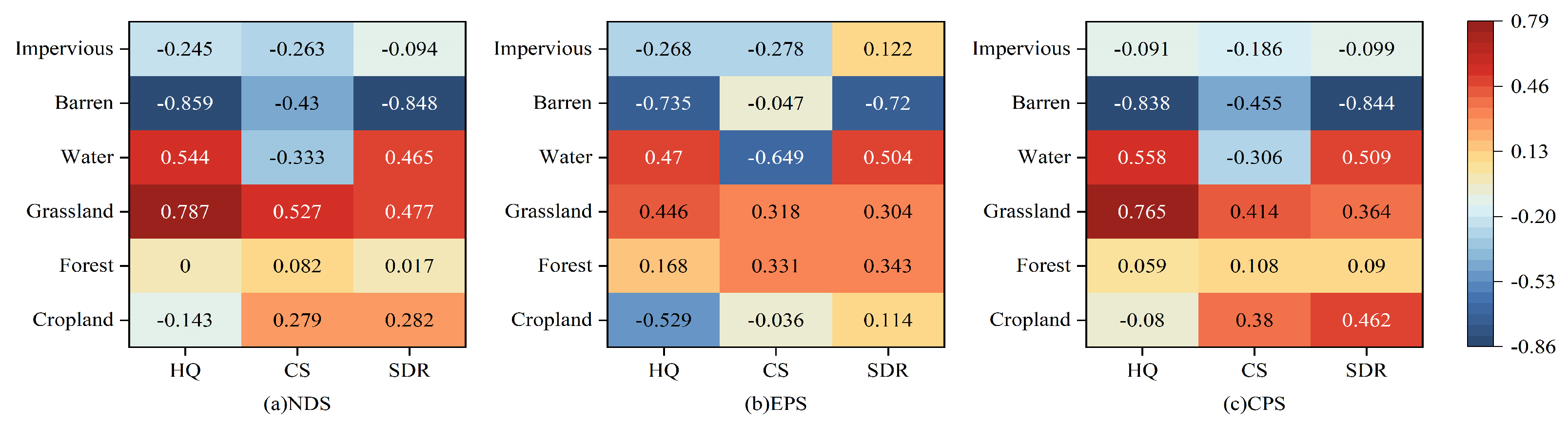
• With positive correlations between habitat quality (r = 0.787), carbon stock (r = 0.527), and soil conservation (r = 0.477), grassland changes dominated the ecosystem service response under the NDS in the analysis of the correlation between land-use types and ecosystem services. The synergistic expansion of grassland and water under the EPS has a certain positive regulating effect on ecosystem functioning in terms of habitat quality (r = 0.446 for grassland; r = 0.47 for water); in the CPS, while the expansion of cropland improves soil conservation (r = 0.462), it worsens grassland degradation, and the correlation between habitat quality and grassland increases to 0.765, highlighting the conflict between trade-offs between ecological functions. This implies that improving the function of regional ecosystem services and achieving sustainable development can be accomplished through land-use optimization focused on ecological conservation.

References

1. Daily, G.C. Nature’s Services: Societal Dependence on Natural Ecosystems; Island Press: Washington, DC, USA, 1997. [Google Scholar]
2. Costanza, R.; d’Arge, R.; De Groot, R.; Farber, S.; Grasso, M.; Hannon, B.; Limburg, K.; Naeem, S.; O’neill, R.V.; Paruelo, J. The value of the world’s ecosystem services and natural capital. Nature 1997, 387, 253–260. [Google Scholar] [CrossRef]
3. Newbold, T.; Hudson, L.N.; Hill, S.L.; Contu, S.; Lysenko, I.; Senior, R.A.; Börger, L.; Bennett, D.J.; Choimes, A.; Collen, B. Global effects of land use on local terrestrial biodiversity. Nature 2015, 520, 45–50. [Google Scholar] [CrossRef] [PubMed]
4. Rao, Y.; Zhou, M.; Ou, G.; Dai, D.; Zhang, L.; Zhang, Z.; Nie, X.; Yang, C. Integrating ecosystem services value for sustainable land-use management in semi-arid region. J. Clean. Prod. 2018, 186, 662–672. [Google Scholar] [CrossRef]
5. Ma, S.; Wen, Z. Optimization of land use structure to balance economic benefits and ecosystem services under uncertainties: A case study in Wuhan, China. J. Clean. Prod. 2021, 311, 127537. [Google Scholar] [CrossRef]
6. Wang, S.; Zheng, X. Dominant transition probability: Combining CA-Markov model to simulate land use change. Environ. Dev. Sustain. 2023, 25, 6829–6847. [Google Scholar] [CrossRef]
7. Verburg, P.H.; Soepboer, W.; Veldkamp, A.; Limpiada, R.; Espaldon, V.; Mastura, S.S. Modeling the spatial dynamics of regional land use: The CLUE-S model. Environ. Manag. 2002, 30, 391–405. [Google Scholar] [CrossRef]
8. Van Dessel, W.; Van Rompaey, A.; Szilassi, P. Sensitivity analysis of logistic regression parameterization for land use and land cover probability estimation. Int. J. Geogr. Inf. Sci. 2011, 25, 489–508. [Google Scholar] [CrossRef]
9. Çağlıyan, A.; Dağlı, D. Monitoring Land Use Land Cover Changes and Modelling of Urban Growth Using a Future Land Use Simulation Model (FLUS) in Diyarbakır, Turkey. Sustainability 2022, 14, 9180. [Google Scholar] [CrossRef]
10. Zhang, D.; Dong, H. Understanding Arable Land change patterns and driving forces in Major Grain-Producing areas: A case study of Sichuan Province using the PLUS Model. Land 2023, 12, 1443. [Google Scholar] [CrossRef]
11. Liu, X.; Liang, X.; Li, X.; Xu, X.; Ou, J.; Chen, Y.; Li, S.; Wang, S.; Pei, F. A future land use simulation model (FLUS) for simulating multiple land use scenarios by coupling human and natural effects. Landsc. Urban Plan. 2017, 168, 94–116. [Google Scholar] [CrossRef]
12. Liang, X.; Liu, X.; Li, X.; Chen, Y.; Tian, H.; Yao, Y. Delineating multi-scenario urban growth boundaries with a CA-based FLUS model and morphological method. Landsc. Urban Plan. 2018, 177, 47–63. [Google Scholar] [CrossRef]
13. Lin, J.; He, P.; Yang, L.; He, X.; Lu, S.; Liu, D. Predicting future urban waterlogging-prone areas by coupling the maximum entropy and FLUS model. Sustain. Cities Soc. 2022, 80, 103812. [Google Scholar] [CrossRef]
14. Zhang, H.; Li, H.; Zhang, J.; Wang, J.; Wang, G.; Shan, Y.; Zheng, H. Simulation of wetland distribution in the Yellow River Basin based on an improved Markov-FLUS model. Environ. Res. Lett. 2024, 19, 104001. [Google Scholar] [CrossRef]
15. Li, H.; Fang, C.; Xia, Y.; Liu, Z.; Wang, W. Multi-scenario simulation of production-living-ecological space in the Poyang Lake area based on remote sensing and RF-Markov-FLUS model. Remote Sens. 2022, 14, 2830. [Google Scholar] [CrossRef]
16. Geng, W.; Li, Y.; Zhang, P.; Yang, D.; Jing, W.; Rong, T. Analyzing spatio-temporal changes and trade-offs/synergies among ecosystem services in the Yellow River Basin, China. Ecol. Indic. 2022, 138, 108825. [Google Scholar] [CrossRef]
17. Sherrouse, B.C.; Clement, J.M.; Semmens, D.J. A GIS application for assessing, mapping, and quantifying the social values of ecosystem services. Appl. Geogr. 2011, 31, 748–760. [Google Scholar] [CrossRef]
18. Villa, F.; Ceroni, M.; Bagstad, K.; Johnson, G.; Krivov, S. ARIES (Artificial Intelligence for Ecosystem Services): A new tool for ecosystem services assessment, planning, and valuation. In Proceedings of the 11th Annual BIOECON Conference on Economic Instruments to Enhance the Conservation and Sustainable Use of Biodiversity, Venice, Italy, 21–22 September 2009. [Google Scholar]
19. Zhang, J.; Zhang, Z.; Liu, L.; Cao, Y.; Zhang, M.; Yuan, Z.; Ma, R.; Liu, X.; Liu, Y. Scaling effects of ecosystem service trade-off and synergy in arid inland river basins: A case study of the Manas River Basin of Xinjiang, China. Ecol. Indic. 2025, 173, 113358. [Google Scholar] [CrossRef]
20. Han, P.; Yang, G.; Wang, Z.; Liu, Y.; Chen, X.; Zhang, W.; Zhang, Z.; Wen, Z.; Shi, H.; Lin, Z. Driving Factors and Trade-Offs/Synergies Analysis of the Spatiotemporal Changes of Multiple Ecosystem Services in the Han River Basin, China. Remote Sens. 2024, 16, 2115. [Google Scholar] [CrossRef]
21. Shen, J.; Zhao, M.; Tan, Z.; Zhu, L.; Guo, Y.; Li, Y.; Wu, C. Ecosystem service trade-offs and synergies relationships and their driving factor analysis based on the Bayesian belief Network: A case study of the Yellow River Basin. Ecol. Indic. 2024, 163, 112070. [Google Scholar] [CrossRef]
22. Li, Y.; Liu, Z.; Li, S.; Li, X. Multi-scenario simulation analysis of land use and carbon storage changes in changchun city based on FLUS and InVEST model. Land 2022, 11, 647. [Google Scholar] [CrossRef]
23. Qiao, X.; Li, Z.; Lin, J.; Wang, H.; Zheng, S.; Yang, S. Assessing current and future soil erosion under changing land use based on InVEST and FLUS models in the Yihe River Basin, North China. Int. Soil Water Conserv. Res. 2024, 12, 298–312. [Google Scholar] [CrossRef]
24. Wang, Y.; Liu, D.; Liang, E.; Ni, J. Structural Characteristics of Endorheic Rivers in the Tarim Basin. Remote Sens. 2022, 14, 4502. [Google Scholar] [CrossRef]
25. Wang, Y.; Wang, Y.; Xia, T.; Li, Y.; Li, Z. Land-use function evolution and eco-environmental effects in the tarim river basin from the perspective of production–living–ecological space. Front. Environ. Sci. 2022, 10, 1004274. [Google Scholar] [CrossRef]
26. Zhang, Q.F.; Chen, Y.N.; Sun, C.J.; Xiang, Y.Y.; Hao, H.C. Changes in Water Storage and Oasis Ecological Security Assessment in the Tarim River Basin. Arid. Land Geogr. 2024, 47, 1–14. [Google Scholar]
27. Aishan, T.; Halik, Ü.; Betz, F.; Tiyip, T.; Ding, J.; Nuermaimaiti, Y. Stand structure and height-diameter relationship of a degraded Populus euphratica forest in the lower reaches of the Tarim River, Northwest China. J. Arid. Land 2015, 7, 544–554. [Google Scholar] [CrossRef]
28. Tang, H.; Wang, L.; Wang, Y. Spatial and Temporal Variation Characteristics of Vegetation Cover in the Tarim River Basin, China, and Analysis of the Driving Factors. Sustainability 2025, 17, 1414. [Google Scholar] [CrossRef]
29. Xu, Z.; Chen, Y.; Li, J. Impact of climate change on water resources in the Tarim River basin. Water Resour. Manag. 2004, 18, 439–458. [Google Scholar] [CrossRef]
30. Zhang, Q.; Xu, C.-Y.; Tao, H.; Jiang, T.; Chen, Y.D. Climate changes and their impacts on water resources in the arid regions: A case study of the Tarim River basin, China. Stoch. Environ. Res. Risk Assess. 2010, 24, 349–358. [Google Scholar] [CrossRef]
31. Guo, H.; Cai, Y.; Yang, Z.; Zhu, Z.; Ouyang, Y. Dynamic simulation of coastal wetlands for Guangdong-Hong Kong-Macao Greater Bay area based on multi-temporal Landsat images and FLUS model. Ecol. Indic. 2021, 125, 107559. [Google Scholar] [CrossRef]
32. Lin, W.; Sun, Y.; Nijhuis, S.; Wang, Z. Scenario-based flood risk assessment for urbanizing deltas using future land-use simulation (FLUS): Guangzhou Metropolitan Area as a case study. Sci. Total Environ. 2020, 739, 139899. [Google Scholar] [CrossRef]
33. Chen, Z.; Huang, M.; Zhu, D.; Altan, O. Integrating remote sensing and a markov-FLUS model to simulate future land use changes in Hokkaido, Japan. Remote Sens. 2021, 13, 2621. [Google Scholar] [CrossRef]
34. Zhang, C.; Wang, P.; Xiong, P.; Li, C.; Quan, B. Spatial pattern simulation of land use based on FLUS model under ecological protection: A case study of Hengyang City. Sustainability 2021, 13, 10458. [Google Scholar] [CrossRef]
35. Zhang, X.R.; Li, A.N.; Nan, X.; Lei, G.; Wang, C. Multi-scenario simulation of land use changes in the China-Pakistan Economic Corridor based on coupled FLUS and SD models. J. Geo-Inf. Sci. 2020, 22, 2393–2409. [Google Scholar] [CrossRef]
36. Sun, W.; Liu, X. Spatio-temporal evolution and multi-scenario prediction of ecosystem carbon storage in Chang-Zhu-Tan Urban agglomeration based on the FLUS-InVEST Model. Sustainability 2024, 16, 7025. [Google Scholar] [CrossRef]
37. Jeong, A.; Kim, M.; Lee, S. Analysis of priority conservation areas using habitat quality models and MaxEnt models. Animals 2024, 14, 1680. [Google Scholar] [CrossRef]
38. Wang, Y.; Sheng, Z.; Wang, H.; Xue, X.; Hu, J.; Yang, Y. Characterization and Multi-Scenario Prediction of Habitat Quality Evolution in the Bosten Lake Watershed Based on the InVEST and PLUS Models. Sustainability 2024, 16, 4202. [Google Scholar] [CrossRef]
39. Wei, Q.; Abudureheman, M.; Halike, A.; Yao, K.; Yao, L.; Tang, H.; Tuheti, B. Temporal and spatial variation analysis of habitat quality on the PLUS-InVEST model for Ebinur Lake Basin, China. Ecol. Indic. 2022, 145, 109632. [Google Scholar] [CrossRef]
40. Yang, H.; Zhang, H.; Wang, Y.; Jia, X.; Hao, L.; Jin, K.; Song, J. Urban bird diversity conservation plan based on the MaxEnt model and InVEST model: A case study of Jinan, China. Ecol. Indic. 2025, 174, 113463. [Google Scholar] [CrossRef]
41. Sharp, R.; Tallis, H.; Ricketts, T.; Guerry, A.; Wood, S.; Chaplin-Kramer, R.; Nelson, E.; Ennaanay, D.; Wolny, S.; Olwero, N.; et al. InVEST 3.2.0 User’s Guide. In The Natural Captial Projest; Stanford University: Stanford, CA, USA; University of Minnesota: Minneapolis-Saint Paul, MN, USA; The Nature Conservancy: Arlington, VA, USA; World Wildlife Fund: Gland, Switzerland, 2017. [Google Scholar]
42. Zhang, X.; Li, M.; Wu, J.; He, Y.; Niu, B. Alpine grassland aboveground biomass and theoretical livestock carrying capacity on the Tibetan Plateau. J. Resour. Ecol. 2022, 13, 129–141. [Google Scholar]
43. Fu, W.; Xia, W.H.; Fan, T.S.; Zhou, Z.; Huo, Y. Scenario projection analysis of ecosystem carbon stocks in the Tarim River Basin. Arid. Land Geogr. 2024, 47, 634–647. [Google Scholar]
44. Jian, Z.; Sun, Y.; Wang, F.; Zhou, C.; Pan, F.; Meng, W.; Sui, M. Soil conservation ecosystem service supply-demand and multi scenario simulation in the Loess Plateau, China. Glob. Ecol. Conserv. 2024, 49, e02796. [Google Scholar] [CrossRef]
45. Wang, X.; Lin, M.; Ding, Z.; Zhou, J.; Wang, C.; Chen, J. Ecological health assessment of Kaikong River Basin based on automatic screening of indicators in Xinjiang. Acta Ecol. Sin. 2020, 40, 4302–4315. [Google Scholar]
46. Wang, Y.; Zhang, Z.; Chen, X. Spatiotemporal change in ecosystem service value in response to land use change in Guizhou Province, southwest China. Ecol. Indic. 2022, 144, 109514. [Google Scholar] [CrossRef]
47. Yang, H.; Zhou, H.; Deng, S.; Zhou, X.; Nie, S. Spatiotemporal variation of ecosystem services value and its response to land use change in the Yangtze river basin, China. Int. J. Environ. Res. 2024, 18, 17. [Google Scholar] [CrossRef]
48. Sun, G.L.; Lu, H.Y.; Zheng, J.X.; Liu, Y.Y.; Ran, Y.J. Spatial-temporal evolution and driving forces of ecological vulnerability in Xinjiang. Arid. Zone Res. 2022, 39, 258–269. [Google Scholar] [CrossRef]
49. Xia, X.X.; Zhu, L.; Yang, A.M.; Jin, H.; Zhang, Q.Q. Evaluation of the Positive and Negative Values of Ecosystem Services Based on the Mountain-Oasis-Desert System (MODS): A Case Study of the Manas River Basin in Xinjiang. Acta Ecol. Sin. 2020, 40, 3921–3934. [Google Scholar]
50. Fu, B. Ecological and environmental effects of land-use changes in the Loess Plateau of China. Chin. Sci. Bull. 2022, 67, 3769–3779. [Google Scholar] [CrossRef]
51. Cao, C.; Luo, Y.; Xu, L.; Xi, Y.; Zhou, Y. Construction of ecological security pattern based on InVEST-Conefor-MCRM: A case study of Xinjiang, China. Ecol. Indic. 2024, 159, 111647. [Google Scholar] [CrossRef]
52. Wu, Y.; Wang, J.; Gou, A. Research on the evolution characteristics, driving mechanisms and multi-scenario simulation of habitat quality in the Guangdong-Hong Kong-Macao Greater Bay based on multi-model coupling. Sci. Total Environ. 2024, 924, 171263. [Google Scholar] [CrossRef]
53. Lei, J.; Zhang, L.; Chen, Z.; Wu, T.; Chen, X.; Li, Y. The impact of land use change on carbon storage and multi-scenario prediction in Hainan Island using InVEST and CA-Markov models. Front. For. Glob. Change 2024, 7, 1349057. [Google Scholar] [CrossRef]
54. Qi, M. Study on Ecosystem Service Functions in Inner Mongolia Autonomous Region Based on PLUS-InVEST Model. Master’s Thesis, Inner Mongolia Agricultural University, Hohhot, China, 2024. [Google Scholar] [CrossRef]
55. Wang, Y.; Feng, Z.Y.; Xu, L.; Gao, W.X. Response of Habitat Quality to Land Use Change and Driving Forces in the Tarim River Basin. Arid. Zone Res. 2024, 41, 2132–2142. [Google Scholar] [CrossRef]
56. Xia, W.; Ma, Y.; Gao, Y.; Huo, Y.; Su, X. Spatial-temporal pattern and spatial convergence of carbon emission intensity of rural energy consumption in China. Environ. Sci. Pollut. Res. 2024, 31, 7751–7774. [Google Scholar] [CrossRef] [PubMed]
57. Wang, C.; Wang, Y.; Wang, R.; Zheng, P. Modeling and evaluating land-use/land-cover change for urban planning and sustainability: A case study of Dongying city, China. J. Clean. Prod. 2018, 172, 1529–1534. [Google Scholar] [CrossRef]
Figure 1. An overview map of the study area. (a) Map of China; (b) line graphs of average annual temperature and average annual precipitation; (c) Elevation maps. Note: review drawing no. GS (2024) 0650.
Sustainability 17 05607 g001
Figure 2. An artificial neural network.
Sustainability 17 05607 g002
Figure 3. Technical flow chart.
Sustainability 17 05607 g003
Figure 4. The distribution of land-use in the TRB, 2000–2023.
Sustainability 17 05607 g004
Figure 5. The land-use distribution in the TRB in 2030 under the following scenarios: (a) 2020; (b) NDS; (c) EPS; and (d) CPS.
Sustainability 17 05607 g005
Figure 6. Chord maps for land-use transfer.
Sustainability 17 05607 g006
Figure 7. The TRB’s habitat quality in 2035 under the following scenarios: (a) 2020, (b) the NDS, (c) the EPS, (d) the CPS, (e) the area of different habitat quality levels in the TRB in 2020, and (fh) the comparison of habitat quality areas of different grades under different scenarios in 2020 and 2035.
Sustainability 17 05607 g007
Figure 8. The TRB’s carbon stock in 2035 under the following scenarios: (a) 2020, (b) the NDS, (c) the EPS, and (d) the CPS.
Sustainability 17 05607 g008
Figure 9. The TRB’s soil conservation in 2035 under the following scenarios: (a) 2020, (b) the NDS, (c) the EPS, and (d) the CPS.
Sustainability 17 05607 g009
Figure 10. The correlation between land-use types and ecosystem services under the following scenarios: (a) the NDS, (b) the EPS, and (c) the CPS.
Sustainability 17 05607 g010
Figure 11. The overall land-use analysis of the TRB.
Sustainability 17 05607 g011
Figure 12. The changes in land usage within the TRB (2020–2035).
Sustainability 17 05607 g012