Abstract
Accurate electricity wholesale price (EWP) forecasting is crucial for advancing sustainability in the energy sector, as it supports more efficient utilization and integration of renewable energy by informing when and how it should be consumed, dispatched, curtailed, or stored. However, high fluctuations in EWP, often resulting from demand–supply imbalances typically caused by sudden surges in electricity usage and the intermittency of renewable energy generation, and unforeseen external events, pose a challenge for accurate forecasting. Incorporating local temporal information (LTI) in time series, such as hourly price changes, is essential for accurate EWP forecasting, as it helps detect rapid market shifts. However, existing methods remain limited in capturing LTI, either relying on point-wise input sequences or, for fixed-length, non-overlapping segmentation methods, failing to effectively model dependencies within and across segments. This paper proposes the Local-Temporal Convolutional Transformer (LT-Conformer) model for day-ahead EWP forecasting, which addresses the challenge of capturing fine-grained LTI using Local-Temporal 1D Convolution and incorporates two attention modules to capture global temporal dependencies (e.g., daily price trends) and cross-feature dependencies (e.g., solar output influencing price). An initial evaluation in the Australian market demonstrates that LT-Conformer outperforms existing state-of-the-art methods and exhibits adaptability in forecasting EWP under volatile market conditions.
1. Introduction
Electricity prices in competitive wholesale markets are subject to substantial fluctuations over time due to the inherent constraints on storage [1]. The inability to efficiently store large quantities of electricity means that supply must closely match demand at all times, leading to variable prices [2,3]. Accurate forecasting of electricity wholesale price (EWP) proves advantageous for diverse stakeholders. It enables energy generators (e.g., those relying on renewable sources) to adjust production schedules, large-scale storage operators to optimize charge and discharge strategies, and load centers to mitigate price exposure through demand-side management [4]. Ultimately, this supports energy sustainability by enabling smarter grid operations [4,5,6], encouraging investment in renewable energy [7], and helping to optimize resource allocation across the power system [6,8].
EWP forecasting has been widely applied to optimize the dispatch of renewables and control large-scale storage in modern electricity grids. In [9], an optimized dispatch strategy is proposed for a hybrid energy system combining photovoltaic, wind, battery, and pumped-storage hydro units in an industrial prosumer case in Portugal. By employing 24 h ahead EWP forecasts, the system dynamically schedules energy resources, reducing operating costs by up to 15% and lowering diesel generator usage from approximately 12% in the rule-based case to around 3% under the optimized dispatch strategy. Study [10] examines wind energy generators in India, where day-ahead EWP forecasts enable smarter bidding and battery scheduling, reducing deviation penalties (charges incurred when actual renewable energy generation deviates from scheduled commitments) by 32%. A stochastic dispatch model in [11] integrates EWP forecasts to manage a multi-energy microgrid, resulting in a 9% cost reduction and a 4% improvement in renewable energy utilization compared with a deterministic baseline. In [12], operational scheduling of behind-the-meter battery systems co-located with solar power is optimized using EWP forecasts, improving renewable self-consumption by around 11% and reducing energy costs by up to 20%.
However, EWP exhibits high volatility and is challenging to forecast since it is impacted by multiple factors (e.g., decision-making across many distinct generators, evolving operational constraints, shifting environmental conditions, infrastructure availability and performance, and demand behavior) across multiple time scales (e.g., seasonal and daily demand patterns, long-term generation availability trends, and sudden outages) [13,14,15,16,17]. One of the primary drivers of short-term fluctuations in EWP is the variability in both demand and supply sides [18,19]. The modern power industry has embraced renewable energy sources, notably wind and solar, as part of its energy portfolio [20,21]. The increasing integration of intermittent renewable energy sources [22] and unforeseen rare events (such as transmission line outages and heatwaves [23]) exacerbate the volatility in the electricity market. Such fluctuations can result in both exceptionally high and low EWP.
Extensive research has explored methods for forecasting market prices. Among those, statistical and machine learning models have captured considerable attention in industry. Statistical models [24,25,26,27,28] utilize mathematical combinations of historical prices and external factors, such as energy generation, load demand, and weather conditions, to forecast EWP. The attractiveness of statistical models lies in their ability to provide physical interpretations for their components, providing operators with insights into the behavior of the models. However, the non-linear and non-stationary nature of price dynamics, coupled with the presence of exogenous factors and rare events, complicates the task of modeling and forecasting effectively. Statistical methods often struggle to capture the intricate patterns and dependencies embedded within EWP data, leading to sub-optimal predictions and heightened uncertainty [29,30]. To overcome the limitations, researchers have increasingly turned to machine learning and deep learning techniques for EWP forecasting. A variety of methods, including Random Forest (RF) [26], Artificial Neural Networks (ANNs) [13,31,32,33], Recurrent Neural Networks (RNNs) [34,35], Long Short-Term Memory (LSTM) networks [36], Convolutional Neural Networks (CNNs) [37,38], and hybrid models [14,39,40,41,42], leverage the foundational models and power of neural networks to capture complex patterns and temporal dependencies within EWP.
The majority of existing machine learning methods approach EWP forecasting as a multivariate time series (MTS) forecasting problem. An MTS consists of multiple interconnected time series with inherent dependencies, characterized by fluctuations and variations over time [43]. These correlations can be classified into three main groups: cross-feature dependencies, local information, and global information within cross-temporal dependencies. Cross-feature dependencies occur when one variable in a time series is influenced by another variable. This acknowledges the interconnected nature of various factors influencing EWP, including supply and demand dynamics, market regulations, weather conditions, and fuel prices, among others. Local information refers to the dependencies and relationships within a short time frame or window. It involves understanding how variables interact within short periods and the temporal patterns in their adjacent areas. For instance, in a daily EWP data set, local information may include price change patterns within hours. Multiple time periods exhibit overlapping and interdependent characteristics, making the task of modeling these variations challenging. Global information encompasses long-range dependencies and relationships spanning over time periods. This involves detecting enduring trends and patterns across extended intervals. Capturing global information enables consideration of periodic effects, revealing variations in EWP across different days or weeks. In recent years, the MTS forecasting methods have increasingly focused on capturing these intricate dependencies to enhance prediction accuracy and reliability.
In terms of MTS forecasting, multiple variant Transformer models [44,45,46,47,48] have been developed due to the advancements in attention mechanisms, which have significantly improved the ability to capture long-range dependencies and relationships within sequential data. Still, existing studies continue to struggle with the challenge of capturing other dependencies. While some studies [44,45,46,47,49] neglect cross-feature dependencies, others [44,45,46] do incorporate cross-temporal dependencies but overlook local information. Incorporating local temporal information is essential for MTS forecasting, particularly for EWP, as it facilitates the detection and analysis of rapid market shifts, thereby enhancing the accuracy of the forecasting model in the presence of unforeseen events that may trigger such fluctuations. Most of these studies, such as Informer [45], and Pyraformer [44], utilize point-wise input sequences to capture temporal dependencies within MTS data. Informer [45] employs ProbSparse self-attention and a distillation-based encoder to capture temporal dependencies. Recent adaptations for EWP forecasting include informer-enhanced variants [50] that incorporate global temporal dependencies to capture periodic trends such as daily, weekly, and seasonal cycles, and hybrid frameworks like MIC-EEMD-Informer [51] that combine signal decomposition with feature selection to capture the nonlinear and multiscale characteristics of EWP series. However, its point-wise input strategy, which computes each time step independently, may still restrict its ability to extract local information in temporal dependencies and risks overlooking critical patterns in the highly volatile EWP series [52]. It has been shown to be beneficial to incorporate information within subseries-level patches or segments to establish dependencies between trajectories across various time steps. For this purpose, studies [43,47,49,53,54,55] embed time series into two-dimensional (2D) vectors for model inputs.
PatchTST [47] integrates a patch design with an attention mechanism to capture temporal dependencies within a single univariate time series, tailored for MTS forecasting. However, it overlooks cross-feature dependencies, a critical factor for MTS forecasting. Crossformer [53] addresses this limitation by dividing the input series into segments and introducing two-stage attention (TSA) layers to capture both cross-temporal and cross-feature dependencies, which has also been leveraged in a recent study on EWP forecasting [56]. DSformer [43] incorporates the concepts from PatchTST and Crossformer, presenting a double sampling transformer architecture that embeds time series into segments. This method captures both local and global information across time and cross-feature dependencies. TimesNet [49] addresses the challenge of modeling local information in complex temporal dependencies by unraveling these variations into multiple intraperiod and interperiod variations. This is achieved by transforming one-dimensional (1D) time series data into 2D tensors based on multiple periods, which allows the model to capture local temporal variations more effectively using 2D CNN kernels. TimeXer [54] captures local information by splitting the endogenous time series into non-overlapping patches, embedding each as a temporal token, and applying self-attention over these tokens to model dependencies across short-term temporal segments. iTransformer [48] treats each variate in an MTS as a single token, resembling an extreme case of patch-based modeling. This design enables attention to capture cross-variable dependencies through learnable embeddings and temporal dependencies via position-wise feed-forward neural networks. WPMixer [55] first decomposes each input time series into multi-resolution wavelet coefficient sequences, then segments each univariate coefficient series into overlapping patches with fixed length, embeds them into a shared latent space, and processes them with a patch mixer to learn localized patterns within each frequency band.
However, existing studies employing the patch/segment-based approach with either a fixed segmentation length, a non-overlapping segmentation strategy, or both for local temporal information extraction face several challenges, as shown in Figure 1a. Overall, there are two main shortcomings: inter-segment dependency misalignment and intra-segment information loss. Inter-segment dependency misalignment, as illustrated in Figure 1a, (1) refers to the lack of correlation or misalignment between different segments or patches. Non-overlapping segmentation with fixed length may cause the partitioned segments (i.e., the red dashed boxes) to be less correlated, leading to local temporal dependencies being captured ineffectively. For instance, a segment spanning 9:00 AM to 12:00 PM may show weak correlation with its neighboring segment from 12:00 PM to 3:00 PM, illustrating inter-segment dependency misalignment, where related patterns across segments are not captured effectively.
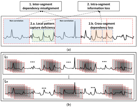
Figure 1.
The shortcomings of existing segment-based methods and our proposed solution: (a) Challenges of non-overlapping segmentation with fixed length. (b) Our idea: overlapping segmentation with varying lengths.
Intra-segment information loss, as illustrated in Figure 1a, (2) is the issue of losing important information or patterns within a single segment. This is further divided into two sub-challenges: (1) Local pattern capture deficiency refers to the difficulty in capturing and modeling local patterns or dependencies within a specific segment. A high correlation between two adjacent time windows is noted in a single patch, as shown in Figure 1a, (2.a). However, dividing time series data into segments of a fixed length may fail to capture this correlation. Within the same example segment mentioned above (9:00 AM to 12:00 PM), local pattern capture deficiency may occur if the correlation between adjacent time intervals, such as 9:15 AM to 9:45 AM and 9:45 AM to 10:15 AM, is not effectively modeled due to insufficient temporal granularity, resulting in the loss of fine-grained temporal dynamics within the segment. (2) Cross-segment dependency loss relates to the inability to effectively capture and model dependencies within subseries that span across segment boundaries, which is highlighted in Figure 1a, (2.b). If a correlation between the period from 8:30 AM to 9:30 AM and another time period exists, the fixed segmentation boundary at 9:00 AM used in the above-mentioned example segment may disrupt this continuity, resulting in cross-segment dependency loss as the dependency spanning across segments is broken.
In practical EWP forecasting, the temporal patterns and dependencies within a data set can span diverse time scales. Crucial information exists within short-term variations, while other important insights may be associated with longer-term trends. One adaptable and flexible idea for time series segmentation, which can accommodate patches of variable lengths, is illustrated in Figure 1b. In simple terms, segments should overlap with their neighbors, and their length should range from Length 1 () to Length n (). This design facilitates the modeling of local patterns with diverse fine-grained temporal resolutions.
Building upon the motivations outlined above, we introduce the Local-Temporal Convolutional Transformer (LT-Conformer) as a novel model for EWP forecasting. The architecture of LT-Conformer comprises three main modules: Local-Temporal 1D CNN (LT-1D CNN), Global-Temporal Attention (GTA), and Cross-Variable Attention (CVA). As is known, CNNs excel at extracting hierarchical features in time series data, capturing local patterns at multiple scales with their variable-sized filters to recognize patterns across different time periods [57,58]. In this context, 1D CNNs are employed to independently convolve over each time series, allowing the model to focus on learning fine-grained local temporal dependencies within individual variables. The LT-1D CNN architecture is designed to leverage 1D convolutional filters of varying sizes over each time series within MTS, alongside multiple kernel sizes, with a stride of one. This design facilitates the capture of local information across a spectrum of scales, thereby providing a more nuanced and detailed feature map that is expected to improve the effectiveness in capturing local temporal dependencies. Leveraging the Transformer with proven capability in handling long-sequence textual data, GTA captures global temporal dependencies, while CVA is adapted to incorporate cross-feature dependencies in the MTS data. Our contributions can be summarized in three key aspects:
- We propose a novel segment-based method to align inter-segment dependencies and preserve intra-segment information, effectively addressing the challenge of capturing local temporal dynamics in EWP forecasting.
- The LT-Conformer represents an advancement in the field of EWP forecasting, specifically designed to capture local temporal patterns, simultaneously integrating global temporal and cross-feature information. By considering the characteristics of EWP, the parameters of the model are tailored to capture relevant features essential for accurate prediction.
- In our experimental evaluations within the Australian market context, the LT-Conformer not only outperforms baseline methods in terms of overall performance but also excels at capturing local temporal dependencies, achieving state-of-the-art (SOTA) results in short-term predictions and showcasing its adeptness at managing the dynamic nature of the energy sector.
2. Proposed Method
2.1. Problem Description
In MTS forecasting, given historical observations , T time steps and N variates, the typical goal is to predict the future S time steps . In our specific context where we focus solely on predicting EWP, the objective simplifies to forecasting future S time steps , using a set of N variates as features, such as grid load demand (GLD) and variable renewable energy (VRE) generation, including wind and solar sources.
EWP can exhibit significant volatility over short and long time-frames, while also often replicating local patterns, such as the typical daily price shape, timing of peak prices, or differences in price profiles between weekdays and weekends, as illustrated in Figure 2. The relationship between EWP, GLD, wind energy generation (WEG), and solar energy generation (SEG) curves suggests the presence of cross-feature dependencies, meaning each variable influences and is influenced by the others. For instance, high WEG or SEG may coincide with low EWP due to the merit order effect (In Australia, the merit order effect refers to the way in which different sources of electricity generation are called upon or dispatched based on their marginal costs [59]. Renewable energy sources, particularly wind and solar, benefit from this due to their minimal costs of generation once the infrastructure (wind turbines or solar panels) is established.) [59,60,61], while high demand may lead to high EWP due to the need for more power generation from expensive sources [15,62,63]. This understanding highlights the importance of incorporating both local and global temporal information as well as cross-feature dependencies into EWP forecasting models.
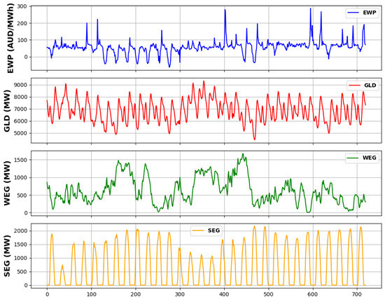
Figure 2.
EWP, GLD, WEG, and SEG at hourly interval in the state of New South Wales, Australia (16 May 2021–14 June 2021) from the Australian Energy Market Operator (AEMO) [64] and Open Platform for National Electricity Market (OpenNEM) [65].
LT-Conformer is designed to capture local temporal information across various scales and manage global temporal and cross-feature dependencies through a combination of components and mechanisms that work in harmony to forecast EWP. The overall architecture and the individual components of the LT-Conformer are presented in the subsequent sections.
2.2. Overview
The overall architecture of the LT-Conformer is shown in Figure 3, which is composed of three main components: the LT-1D CNN module, the GTA module, and the CVA module.
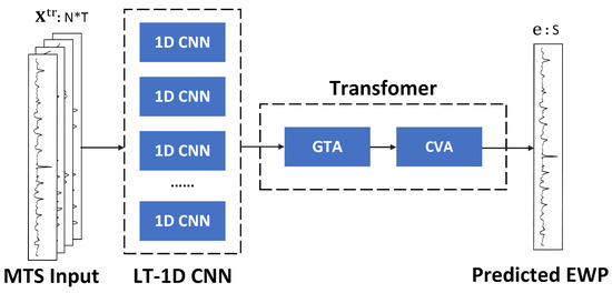
Figure 3.
Overall architecture of LT-Conformer.
The LT-1D CNN module is responsible for extracting local temporal features from the input MTS data. It consists of multiple 1D CNN layers, each of which applies 1D convolutional filters to capture patterns and dependencies within the time dimension. By using multiple 1D CNN layers with different kernel sizes, the model can effectively capture local patterns at various time scales.
The output of the LT-1D CNN module is then fed into the Transformer module, which incorporates two attention mechanisms: GTA and CVA. These attention mechanisms, as derived from the TSA module in the Crossformer architecture [53], enable the model to capture long-range dependencies and interactions within the MTS data. The GTA mechanism allows the model to attend to relevant time steps across the entire time series, enabling it to capture global temporal patterns and dependencies. This is particularly useful for EWP forecasting, where events at different time points can influence future behaviors. The CVA mechanism facilitates capturing dependencies and interactions across various variables or features in MTS data, which is crucial as complex interdependencies are often present among variables.
2.3. Local-Temporal 1D CNN Module
In order to incorporate local temporal dependencies for MTS forecasting more effectively, we propose an overlapping patch-based method with non-fixed lengths. Indeed, the proposed method is designed to manage local information along with its overlapping patterns within specific time periods. This method essentially breaks down the time series into smaller, overlapping patches or segments, each of which captures local temporal patterns. Allowing these patches to overlap ensures continuity and captures the dependencies between adjacent time periods. By allowing for varying patch lengths within a predefined range, which is optimized through grid search, the model can adapt to capture patterns and trends that occur over varying lengths of time.
Note that CNNs are widely applied in the computer vision field [66,67] and have also been effectively adapted for time series data [49,58,68,69,70]. They are proficient in learning hierarchical features within data [57,58,71]. In time series analysis, this capability allows them to capture local patterns and dependencies through their convolutional filters, which scan the input data and extract localized features. Additionally, CNNs can be designed with filters of varying sizes, which enables them to analyze the data at multiple scales or resolutions [72,73]. This is particularly useful for capturing patterns that occur over different time periods.
As shown in Figure 4, 1D convolutional filters of varying sizes are applied across the MTS data, with a stride of one. Specifically, a kernel size represented as enables the model to integrate information across a 2-h span, while a kernel extends this to 3 h, and so on. The underlying idea is that larger kernels have the potential to integrate information over more extended temporal intervals, thus capturing longer local temporal dependencies. The approach is designed to capture local dependencies and extract features from different temporal contexts within the time series. Consequently, the convolutional process is expected to yield feature maps of various dimensions. Given the transposed input MTS data , the convolutional operation can be formulated as follows:
where N is the number of features and T is the number of time steps. is the number of filters for the kernel size . is the 1D convolutional kernel of size . denotes the 1D convolutional operation between input and kernel with a stride of 1 along the time dimension. The ReLU activation function is applied to the output of the convolutional operation, introducing non-linearity to the feature maps as follows:
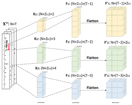
Figure 4.
The architecture of LT-1D CNN.
is further reshaped from a 2D feature map to a 3D tensor, resulting in a flattened feature vector as , preserving the feature and time information in a flattened format as follows:
2.4. Global-Temporal Attention Module
In this module, we input different sizes of flattened feature maps to the multi-head self-attention (MSA):
where is the MSA mechanism applied along the time dimension, taking as the query, key, and value inputs. is an intermediate tensor obtained after applying the MSA mechanism and layer normalization to . MLP represents a multi-layer perceptron applied to . is the final output tensor after applying the MLP and another layer normalization to .
2.5. Cross-Variable Attention Module
Compared with the TSA approach [53], which employs a routing mechanism to extract dimensional features for complexity reduction, our CVA module applies MSA directly to to avoid the potential noise introduced by the utilization of a routing matrix:
where is the MSA mechanism applied along the feature dimension, taking as the query, key, and value inputs. is the tensor obtained after applying layer normalization to the sum of and . is the final output tensor after applying the MLP and another layer normalization to .
3. Experiment
3.1. Data Sets
To assess the performance of the LT-Conformer model for EWP forecasting, this study has selected two states in Australia: New South Wales (NSW) and South Australia (SA). The selection of these regions for our case study aims to validate the ability of the LT-Conformer model in both conventional and renewable-centric energy markets.
The penetration of electricity generation by each type of energy source in both regions from 2021 to 2023 is shown in Figure 5. NSW, located in the south-eastern region of Australia, is the most populous state and relies heavily on non-renewable energy sources, such as coal and gas energy, which accounted for approximately 70.5% of total electricity generation during this period, as shown in Figure 5a. Conversely, SA, situated in the southern central part of the country, predominantly generates its electricity from renewable sources, including wind and solar, which together contributed around 71.3% of electricity generation in the region over the same timeframe, as shown in Figure 5b. The inherent intermittency of these renewable sources contributes to greater variability in electricity production, which is reflected by a higher standard deviation and fluctuation in EWP in SA compared with NSW. The data sets encompass a temporal span from 1 May 2021 to 23 November 2023, comprising data points collected at hourly intervals.
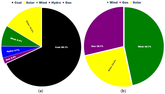
Figure 5.
Different types of sources for electricity generation in NSW (a) and SA (b).
For this initial analysis of LT-Conformer, we limit the input feature space to four key variables: EWP, GLD, and generation from VRE sources, specifically WEG and SEG. Those data, obtained from the AEMO platform [64] and OpenNEM platform [65], are well-validated and used in other published work [15,16,17].
The four variables have been selected for their strong influence on price in the Australian market. Variations in GLD are a primary determinant of market-clearing prices; higher demand levels typically lead to the dispatch of higher-cost generation units, thereby increasing wholesale prices, especially during peak periods [30]. Conversely, during low-demand periods, surplus generation may drive prices down or even result in negative pricing under high renewable output [30]. WEG and SEG, due to their weather-dependent and limited controllability, introduce significant short-term variability in supply. This intermittency can lead to rapid imbalances between generation and demand, resulting in price volatility [21,30]. In particular, sudden drops in VRE output may necessitate the rapid dispatch of higher-cost backup generators, while unexpected surpluses may suppress prices or even lead to negative pricing under low demand conditions [21,60].
The focus of this work is to examine how model design impacts EWP forecasting performance and how such design can be tailored to maximize accuracy. We note that further performance improvements may be realized by tuning and/or expanding the input feature set (e.g., incorporating weather data and forecasts, import/export capacities of interconnected systems, fuel price information, etc.). This remains an important area for future work that would complement the model design focus of this study.
There are some extreme price spikes possibly due to socio-political events, transmission line outages, or severe weather conditions. For the scope of this study, we are not focused on forecasting the presence of extreme price events, so we impose a ceiling and floor on electricity prices within a specified threshold. Following widely adopted practice in existing EWP forecasting literature [15,74,75,76], this capping method serves two primary purposes within the modeling process. First, it mitigates the influence of extreme outliers, which may distort the loss function during model training and lead to biased parameter estimation. Second, it facilitates fair and consistent model evaluation by constraining the analysis to typical price ranges that reflect standard market dynamics. For both NSW and SA, we define the price range as [−600, 600] AUD/MWh and set that any electricity price falling below this range is capped at −600 AUD/MWh, and any price exceeding the range is capped at 600 AUD/MWh. This capping method was applied to only around 1% of the total samples examined for both states.
3.2. Experimental Setup
We selected the Mean Absolute Error (MAE), Root Mean Squared Error (RMSE), and Symmetric Mean Absolute Percentage Error (SMAPE) as the evaluation metrics.
where and are the actual and predicted values at the i-th time point, for each of the n observations.
To conduct a comparative analysis and verify the effectiveness of the LT-Conformer, we have chosen both classical and SOTA models, known for their strong performance in short-term time series forecasting, specifically in the application of EWP prediction. These models include the Linear Regression (LR) model [28], Crossformer [53], Informer [45], TimesNet [49], PatchTST [47], iTransformer [48], and WPMixer [55].
The data set is divided into samples, each encompassing 24 hourly input features along with the next 24 h of EWP as prediction targets. These samples with distinct input–output pairings are generated by sliding a 1-h window across the entire data set, which results in 22,440 samples for each state. We adopt 5-fold cross-validation by randomly partitioning the samples into 80% for training and 20% for testing. The overall experimental results presented are the average results across these five testing sets. Other reported results are also based on evaluations across all testing sets.
We employed the grid search method to fine-tune the hyperparameter dimensions of our model, which include kernel size, number of channels, attention heads, encoder layers, dropout ratios, and learning rate, among others. To determine the optimal configuration of the varying-length convolutional kernels in the LT-1D CNN module, we systematically evaluated a range of kernel size combinations. The search began with shorter sequences starting from {, } and gradually extended to more comprehensive sets (e.g., {, , }, {, , , }, …), up to {, , …, }, enabling the model to capture local temporal patterns across multiple scales. For each kernel size in a given combination, the number of output channels was chosen from [2, 4, 8], and all possible channel size configurations were evaluated. For example, for the kernel set {, , }, configurations such as {2, 2, 2}, {4, 2, 2}, {2, 4, 2}, and so on, up to {8, 8, 8}, were tested. The final configuration was selected based on the best validation performance. The optimal hyperparameter values for the LT-Conformer in both states are presented in Table 1. Similarly, for benchmarking purposes, we conducted a grid search optimization for the baseline models, calibrated specifically for EWP forecasting, to ensure the identification of the most performant parameter configurations. The “MinMaxScaler” [77] normalization function was employed in both the pre-processing and post-processing stages. We also undertook denormalization, which is critical for ensuring that the evaluation metric reflects the true scale of the data.

Table 1.
Optimal hyperparameters of LT-Conformer for EWP forecasting in NSW and SA.
3.3. Comparative Results on Forecasting Performance
3.3.1. Overall Results
The performance of all methods was evaluated using MAE, RMSE, and SMAPE in NSW and SA, as shown in Table 2. Overall, the LT-Conformer model consistently outperforms the other forecasting methods in both regions, demonstrating minimal error across all evaluated metrics. To evaluate whether the performance improvements of the LT-Conformer are statistically significant compared with all selected models, we conduct paired t-tests at the 0.05 significance level using the MAE. The results in Table 2 show that the LT-Conformer significantly outperforms all compared methods across both regions, with all corresponding p-values below 0.001. Although the MAE difference between the LT-Conformer and Informer is smaller than that with other models, the LT-Conformer achieves consistently lower errors across most samples in NSW, resulting in a larger t-statistic. Figure 6 highlights model performance on selected days in NSW and SA with both high and low EWP variability. These example cases were chosen because they are broadly representative of the observed trends on days with high and low variations for each state. The figure shows that LT-Conformer more accurately tracks EWP values, even in the presence of price spikes. As noted in Figure 6a,c, the LT-Conformer model (represented by the dashed red line) closely tracks the actual EWP values (solid black line), demonstrating its ability to accurately capture the fluctuations and spikes in the EWP. It is worth noting that the Informer model (represented by the dash-dot blue line) also exhibits some ability to track the actual EWP patterns. Other models exhibit larger deviations from the actual EWP values, particularly during the peak hours of the day. While there are some deviations, the LT-Conformer model can capture both positive and negative actual EWP values more accurately than the other models, closely following the rise and fall of prices throughout the day. In Figure 6b,d, the actual EWP data show a relatively flat trend without large variations across the whole day. The LT-Conformer model also achieves superior results compared with the other SOTA methods. These results demonstrate the adaptability of LT-Conformer in forecasting EWP and accurately tracking actual data, whether it shows large fluctuations or remains relatively steady.
Table 2.
Overall performance of LT-Conformer and baseline models based on average MAE, RMSE, and SMAPE, along with paired t-test results (t-statistic) for MAE (p < 0.001 for all comparative models).
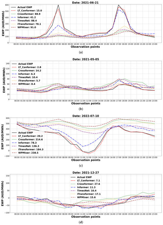
Figure 6.
Forecasting results with MAE in four example cases: EWP with large variation in NSW (a) and SA (c); EWP with small variation in NSW (b) and SA (d).
3.3.2. Results for Varying Levels and Volatility of EWP and REG
To provide insights into the robustness and adaptability of the models across diverse market conditions, a performance analysis on forecasting accuracy was conducted for various levels and volatilities of both EWP and REG in NSW and SA. This analysis specifically targeted forecasting accuracy across the values and volatility of both EWP and REG, categorized as low, medium, and high based on their average values and separately standard deviations over the 24 h test period. Each category represented one-third of the data range, corresponding to the lower, middle, and upper thirds, respectively.
The performance of the models across the defined ranges in both EWP values and EWP volatility is shown in Figure 7 and Figure 8, while the corresponding results for REG values and REG volatility are presented in Figure 9 and Figure 10. The LT-Conformer model exhibits the lowest MAE values across all three categories under diverse market conditions and renewable output scenarios in both regions, demonstrating its forecasting performance and adaptability.
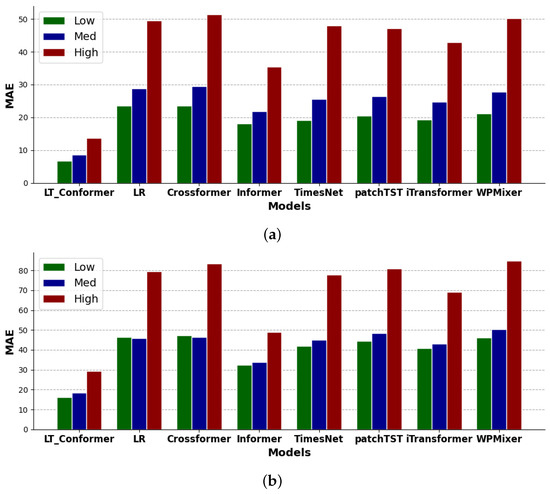
Figure 7.
Performance comparison on EWP forecasting across low, medium, and high values in NSW (a) and SA (b).
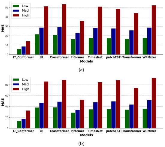
Figure 8.
Performance comparison on EWP forecasting across low, medium, and high volatility in NSW (a) and SA (b).
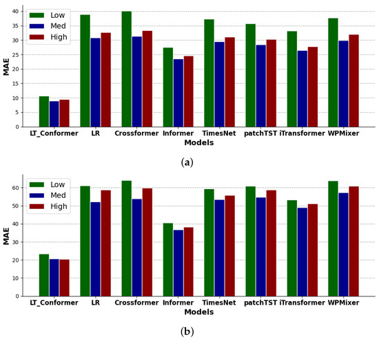
Figure 9.
Performance comparison on EWP forecasting across low, medium, and high values of REG in NSW (a) and SA (b).
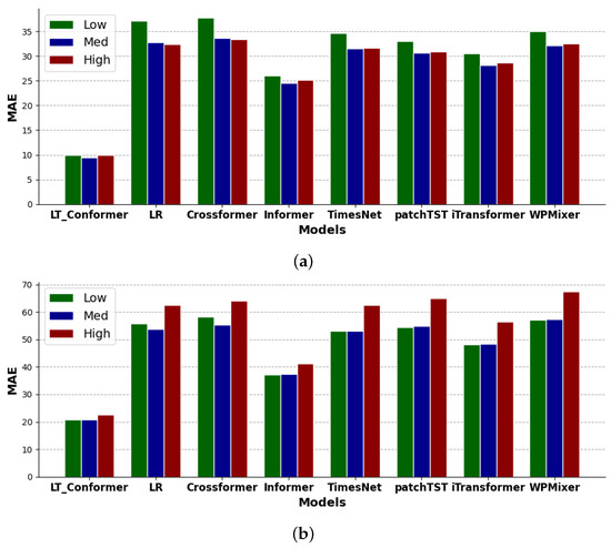
Figure 10.
Performance comparison on EWP forecasting across low, medium, and high volatility of REG in NSW (a) and SA (b).
In terms of levels of EWP and REG, the LT-Conformer model demonstrates high forecasting accuracy under low EWP values, corresponding to market conditions such as off-peak times with low GLD [18,19], and under low REG values, which typically occur at night for solar or during periods of low wind conditions. As EWP and REG values increase to medium levels, the model continues to perform effectively, adapting to the standard market dynamics characterized by a balanced supply-demand scenario, while also maintaining accuracy under medium REG values associated with typical daytime renewable output. In high EWP and REG value scenarios, the model adapts well to periods of price spikes as well as peak solar or wind output.
When evaluating the volatility of EWP and REG, the LT-Conformer performs well in forecasting EWP under low price variation scenarios, effectively capturing stable market conditions, and under low REG volatility, such as during consistently sunny or windy periods with stable renewable output. It maintains this performance under medium levels of price and REG volatility, handling typical market variations and routine fluctuations in solar and wind output adeptly. Even in cases of high price and REG volatility, the LT-Conformer outperforms other models, showcasing its robustness in tracking significant price movements and adapting to rapid changes in renewable output, such as sudden drops in solar output due to cloud cover or fluctuations in wind speed.
3.4. Effectiveness of Local Temporal 1D CNN
In this analysis, we aim to explore the capability of LT-Conformer to capture local temporal dynamics within EWP. We are particularly interested in understanding the short-term (e.g., 2–4 h) fluctuations in EWP and their implications over extended periods. This forms part of a post-hoc analysis conducted on the predictions of the model over the test data set. To achieve this, we first compute the absolute differences between adjacent time points to quantify immediate changes within the test data sets. For the initial time point in the time series, we address potential boundary issues by substituting the median of the computed differences, ensuring a robust starting point for our analysis. Given a time series in test data sets , the difference at each time point t is calculated as follows:
To capture changes over a period of p hours (where p is an integer greater than 1), the average of adjacent differences is considered:
where represents the change over a p-hour period at time t.
Temporal differences within EWP are classified into three distinct levels of fluctuation. Upon examining the differences over a p-hour interval, we compute the average MAE for low, medium, and high fluctuation levels, denoted as , , and , respectively, which correspond to the lower, middle, and upper thirds of the EWP value distribution. The experiment compares the LT-Conformer model with other baseline models in NSW and SA, as shown in Table 3. The LT-Conformer model exhibits substantially lower MAE compared with the other models across different levels of local EWP variability over our three variability measurement periods. This indicates that the LT-Conformer model is more robust to extreme fluctuations and volatility in the short term, due to the ability of the LT-1D CNN to effectively capture and model local temporal patterns, even during periods of high variability. Additionally, LT-Conformer demonstrates stability in performance across varying local EWP variability.
Table 3.
Performance comparison based on average MAE across different levels of local EWP variability for 2 h, 3 h, and 4 h measurement periods.
While comparative models perform worse than LT-Conformer across varying conditions, some show relatively stronger performance among themselves. Among patch-based methods, TimesNet [49] stands out, effectively capturing multi-scale temporal patterns through temporal basis decomposition while maintaining variable-wise context. iTransformer [48], viewed as an extreme case of patch-based design, also performs well by treating each variate as a token, allowing the efficient modeling of cross-variable dependencies and preserving temporal dynamics via position-wise feed-forward encoding and instance normalization. In contrast, Crossformer [53] performs poorly under high variability, likely due to its inflexible segmentation being less adaptable to the spiky and non-stationary nature of EWP. Interestingly, the point-wise model Informer [45] remains competitive, outperforming patch-based models. This suggests that when patch-based methods are not carefully aligned with the characteristics of the EWP, they may underperform compared with well-designed point-wise models.
4. Conclusions
This study introduces the LT-Conformer, a novel model for MTS forecasting, which exhibits SOTA performance on day-ahead EWP prediction in the Australian energy market, known for its significant volatility and rapid intraday price spikes. The LT-Conformer utilizes an LT-1D CNN to effectively align inter-segment dependency and preserve intra-segment information, which is crucial for capturing local temporal information. The architecture extracts and integrates both local and global temporal features and cross-feature interactions.
Empirical evaluations show LT-Conformer consistently outperforms contemporary models in our preliminary study of two Australian electricity systems. Indeed, the best performing comparative model has an MAE that is 2.6 times higher than LT-Conformer in NSW and 1.8 times higher in SA. The robustness and adaptability of the model are confirmed through comparative analyses. Notably, the LT-Conformer performs well across different EWP and fluctuation levels, indicating its versatility in forecasting across stable, dynamic, and volatile market scenarios.
While preliminary results on our two case study networks look promising, further validation is required to explore the generalizability of LT-Conformer. To that end, future work should test the model across markets in diverse geographical regions to broaden its applicability. Additionally, evaluating its performance on various MTS data sets from different application domains will help assess its generalization capability. Future work will also concentrate on enhancing the performance of the LT-Conformer for EWP prediction through more sophisticated feature engineering and integration of a wider set of relevant features. Finally, it would be valuable to compare the performance of LT-Conformer against other forecasting methods in real-time EWP operational settings, particularly in settings where data may be less reliable and/or where energy market participants employ their commercial forecasting solutions. Such validation is an interesting and important avenue for future work.
Author Contributions
Conceptualization, B.Z., H.T., A.B. and A.C.R.; methodology, B.Z., H.T., A.B. and A.C.R.; software, B.Z.; validation, B.Z., H.T. and A.B.; formal analysis, B.Z., H.T., A.B. and A.C.R.; investigation, B.Z., H.T., A.B. and A.C.R.; data curation, B.Z.; writing—original draft preparation, B.Z.; writing—review and editing, B.Z., H.T., A.B. and A.C.R.; visualization, B.Z.; supervision, H.T., A.B. and A.C.R.; project administration, H.T., A.B. and A.C.R.; funding acquisition, H.T., A.B. and A.C.R. All authors have read and agreed to the published version of the manuscript.
Funding
This study received funding from the RACE for 2030 Cooperative Research Centre, with support from Buildings Alive Pty Ltd. and the University of Technology Sydney.
Institutional Review Board Statement
Not applicable.
Informed Consent Statement
Not applicable.
Data Availability Statement
Data are contained within the article.
Conflicts of Interest
Author A. Craig Roussac is currently employed by Buildings Alive Pty Ltd. The remaining authors declare that the research was conducted in the absence of any commercial or financial relationships that could be construed as a potential conflict of interest. The authors declare that this study received funding from Buildings Alive Pty Ltd. The funder was not involved in the study design, collection, analysis, interpretation of data, the writing of this article or the decision to submit it for publication.
References
- Sgarlato, R.; Ziel, F. The Role of Weather Predictions in Electricity Price Forecasting Beyond the Day-Ahead Horizon. IEEE Trans. Power Syst. 2022, 38, 2500–2511. [Google Scholar] [CrossRef]
- Mousavi, F.; Nazari-Heris, M.; Mohammadi-Ivatloo, B.; Asadi, S. Energy market fundamentals and overview. In Energy Storage in Energy Markets; Elsevier: Amsterdam, The Netherlands, 2021; pp. 1–21. [Google Scholar]
- Stawska, A.; Romero, N.; de Weerdt, M.; Verzijlbergh, R. Demand response: For congestion management or for grid balancing? Energy Policy 2021, 148, 111920. [Google Scholar] [CrossRef]
- Wang, K.; Xu, C.; Zhang, Y.; Guo, S.; Zomaya, A.Y. Robust Big Data Analytics for Electricity Price Forecasting in the Smart Grid. IEEE Trans. Big Data 2017, 5, 34–45. [Google Scholar] [CrossRef]
- Daly, J.; Zheng, L.; Xuan, M.; Yang, Y.; De Rosa, M.; Pallonetto, F. Comparative analyses of forecasting techniques for electricity wholesale price under high penetration of renewable energy systems. In Proceedings of the IET Conference Proceedings CP821, Valletta, Malta, 7–9 November 2022; pp. 520–525. [Google Scholar]
- Anwar, M.; Naeem, A.; Gul, H.; Arif, A.; Fareed, S.; Javaid, N. Electricity Price and Load Forecasting Using Data Analytics in Smart Grid: A Survey. In Proceedings of the Advances in Internet, Data and Web Technologies: The 8th International Conference on Emerging Internet, Data and Web Technologies (EIDWT-2020), Kitakyushu, Japan, 24–26 February 2020; Springer: Cham, Switzerland, 2020; pp. 427–439. [Google Scholar]
- Pikus, M.; Wąs, J. Predictive modeling of renewable energy purchase prices using deep learning based on polish power grid data for small hybrid PV microinstallations. Energies 2024, 17, 628. [Google Scholar] [CrossRef]
- Li, G.; Lawarree, J.; Liu, C.C. State-of-the-Art of Electricity Price Forecasting in a Grid Environment. In Handbook of Power Systems II; Springer: Berlin/Heidelberg, Germany, 2010; pp. 161–187. [Google Scholar]
- Bento, P.; Nunes, H.; Pombo, J.; Calado, M.d.R.; Mariano, S. Daily Operation Optimization of a Hybrid Energy System Considering a Short-Term Electricity Price Forecast Scheme. Energies 2019, 12, 924. [Google Scholar] [CrossRef]
- Abhinav, R.; Pindoriya, N.M. Electricity Price Forecast for Optimal Energy Management for Wind Power Producers: A Case Study in Indian Power Market. In Proceedings of the 2018 IEEE Innovative Smart Grid Technologies-Asia (ISGT Asia), Singapore, 22–25 May 2018; pp. 1233–1238. [Google Scholar]
- Houben, N.; Cosic, A.; Stadler, M.; Mansoor, M.; Zellinger, M.; Auer, H.; Ajanovic, A.; Haas, R. Optimal dispatch of a multi-energy system microgrid under uncertainty: A renewable energy community in Austria. Appl. Energy 2023, 337, 120913. [Google Scholar] [CrossRef]
- Chitsaz, H.; Zamani-Dehkordi, P.; Zareipour, H.; Parikh, P.P. Electricity Price Forecasting for Operational Scheduling of Behind-the-Meter Storage Systems. IEEE Trans. Smart Grid 2017, 9, 6612–6622. [Google Scholar] [CrossRef]
- Pino, R.; Parreno, J.; Gomez, A.; Priore, P. Forecasting next-day price of electricity in the Spanish energy market using artificial neural networks. Eng. Appl. Artif. Intell. 2008, 21, 53–62. [Google Scholar] [CrossRef]
- Kuo, P.H.; Huang, C.J. An Electricity Price Forecasting Model by Hybrid Structured Deep Neural Networks. Sustainability 2018, 10, 1280. [Google Scholar] [CrossRef]
- Beltrán, S.; Castro, A.; Irizar, I.; Naveran, G.; Yeregui, I. Framework for collaborative intelligence in forecasting day-ahead electricity price. Appl. Energy 2022, 306, 118049. [Google Scholar] [CrossRef]
- Nogales, F.; Contreras, J.; Conejo, A.; Espinola, R. Forecasting next-day electricity prices by time series models. IEEE Trans. Power Syst. 2002, 17, 342–348. [Google Scholar] [CrossRef]
- Cruz, A.; Muñoz, A.; Zamora, J.L.; Espínola, R. The effect of wind generation and weekday on Spanish electricity spot price forecasting. Electr. Power Syst. Res. 2011, 81, 1924–1935. [Google Scholar] [CrossRef]
- Asif, M.; Muneer, T. Energy supply, its demand and security issues for developed and emerging economies. Renew. Sustain. Energy Rev. 2007, 11, 1388–1413. [Google Scholar] [CrossRef]
- Guo, Z.; Xu, W.; Yan, Y.; Sun, M. How to realize the power demand side actively matching the supply side?—A virtual real-time electricity prices optimization model based on credit mechanism. Appl. Energy 2023, 343, 121223. [Google Scholar] [CrossRef]
- Dincer, I. Renewable energy and sustainable development: A crucial review. Renew. Sustain. Energy Rev. 2000, 4, 157–175. [Google Scholar] [CrossRef]
- Hua, Y.; Oliphant, M.; Hu, E.J. Development of renewable energy in Australia and China: A comparison of policies and status. Renew. Energy 2016, 85, 1044–1051. [Google Scholar] [CrossRef]
- Fornasiero, P.; Graziani, M. Renewable Resources and Renewable Energy: A Global Challenge; CRC Press: Boca Raton, FL, USA, 2011. [Google Scholar]
- Miller, M. Preliminary Report NSW and Victoria Separation Event 4 January 2020. Available online: https://www.aemo.com.au/-/media/files/electricity/nem/market_notices_and_events/power_system_incident_reports/2020/preliminary-report-nsw-and-victoria-separation-event-4-jan-2020.pdf?la=en (accessed on 15 November 2023).
- Koopman, S.J.; Ooms, M.; Carnero, M.A. Periodic Seasonal Reg-ARFIMA-GARCH Models for Daily Electricity Spot Prices. J. Am. Stat. Assoc. 2007, 102, 16–27. [Google Scholar] [CrossRef]
- Gonzalez, V.; Contreras, J.; Bunn, D.W. Forecasting Power Prices Using a Hybrid Fundamental-Econometric Model. IEEE Trans. Power Syst. 2011, 27, 363–372. [Google Scholar] [CrossRef]
- Mei, J.; He, D.; Harley, R.; Habetler, T.; Qu, G. A Random Forest Method for Real-Time Price Forecasting in New York Electricity Market. In Proceedings of the 2014 IEEE PES General Meeting|Conference & Exposition, National Harbor, MD, USA, 27–31 July 2014; pp. 1–5. [Google Scholar]
- Schütz Roungkvist, J.; Enevoldsen, P.; Xydis, G. High-resolution electricity spot price forecast for the Danish power market. Sustainability 2020, 12, 4267. [Google Scholar] [CrossRef]
- Ulgen, T.; Poyrazoglu, G. Predictor Analysis for Electricity Price Forecasting by Multiple Linear Regression. In Proceedings of the 2020 International Symposium on Power Electronics, Electrical Drives, Automation and Motion (SPEEDAM), Sorrento, Italy, 24–26 June 2020; pp. 618–622. [Google Scholar]
- Lago, J.; Marcjasz, G.; De Schutter, B.; Weron, R. Forecasting day-ahead electricity prices: A review of state-of-the-art algorithms, best practices and an open-access benchmark. Appl. Energy 2021, 293, 116983. [Google Scholar] [CrossRef]
- Weron, R. Electricity price forecasting: A review of the state-of-the-art with a look into the future. Int. J. Forecast. 2014, 30, 1030–1081. [Google Scholar] [CrossRef]
- Bunn, D.W. Forecasting loads and prices in competitive power markets. Proc. IEEE 2000, 88, 163–169. [Google Scholar] [CrossRef]
- Mandal, P.; Senjyu, T.; Funabashi, T. Neural networks approach to forecast several hour ahead electricity prices and loads in deregulated market. Energy Convers. Manag. 2006, 47, 2128–2142. [Google Scholar] [CrossRef]
- Amjady, N. Day-ahead price forecasting of electricity markets by a new fuzzy neural network. IEEE Trans. Power Syst. 2006, 21, 887–896. [Google Scholar] [CrossRef]
- Anbazhagan, S.; Kumarappan, N. Day-Ahead Deregulated Electricity Market Price Forecasting Using Recurrent Neural Network. IEEE Syst. J. 2012, 7, 866–872. [Google Scholar] [CrossRef]
- Zhang, C.; Li, R.; Shi, H.; Li, F. Deep learning for day-ahead electricity price forecasting. IET Smart Grid 2020, 3, 462–469. [Google Scholar] [CrossRef]
- Khalid, R.; Javaid, N.; Al-Zahrani, F.A.; Aurangzeb, K.; Qazi, E.u.H.; Ashfaq, T. Electricity Load and Price Forecasting Using Jaya-Long Short Term Memory (JLSTM) in Smart Grids. Entropy 2019, 22, 10. [Google Scholar] [CrossRef]
- Khan, Z.A.; Fareed, S.; Anwar, M.; Naeem, A.; Gul, H.; Arif, A.; Javaid, N. Short Term Electricity Price Forecasting Through Convolutional Neural Network (CNN). In Web, Artificial Intelligence and Network Applications, Proceedings of the Workshops of the 34th International Conference on Advanced Information Networking and Applications (WAINA-2020), Caserta, Italy, 15–17 April 2020; Springer: Cham, Switzerland, 2020; pp. 1181–1188. [Google Scholar]
- Aslam, S.; Ayub, N.; Farooq, U.; Alvi, M.J.; Albogamy, F.R.; Rukh, G.; Haider, S.I.; Azar, A.T.; Bukhsh, R. Towards Electric Price and Load Forecasting Using CNN-Based Ensembler in Smart Grid. Sustainability 2021, 13, 12653. [Google Scholar] [CrossRef]
- Tan, Y.Q.; Shen, Y.X.; Yu, X.Y.; Lu, X. Day-ahead electricity price forecasting employing a novel hybrid frame of deep learning methods: A case study in NSW, Australia. Electr. Power Syst. Res. 2023, 220, 109300. [Google Scholar] [CrossRef]
- Huang, S.; Shi, J.; Wang, B.; An, N.; Li, L.; Hou, X.; Wang, C.; Zhang, X.; Wang, K.; Li, H.; et al. A hybrid framework for day-ahead electricity spot-price forecasting: A case study in China. Appl. Energy 2024, 373, 123863. [Google Scholar] [CrossRef]
- Ghimire, S.; Deo, R.C.; Casillas-Pérez, D.; Sharma, E.; Salcedo-Sanz, S.; Barua, P.D.; Acharya, U.R. Half-hourly electricity price prediction with a hybrid convolution neural network-random vector functional link deep learning approach. Appl. Energy 2024, 374, 123920. [Google Scholar] [CrossRef]
- Parizad, B.; Ranjbarzadeh, H.; Jamali, A.; Khayyam, H. An Intelligent Hybrid Machine Learning Model for Sustainable Forecasting of Home Energy Demand and Electricity Price. Sustainability 2024, 16, 2328. [Google Scholar] [CrossRef]
- Yu, C.; Wang, F.; Shao, Z.; Sun, T.; Wu, L.; Xu, Y. Dsformer: A double sampling transformer for multivariate time series long-term prediction. In Proceedings of the 32nd ACM International Conference on Information and Knowledge Management, Birmingham, UK, 21–25 October 2023; pp. 3062–3072. [Google Scholar]
- Liu, S.; Yu, H.; Liao, C.; Li, J.; Lin, W.; Liu, A.X.; Dustdar, S. Pyraformer: Low-Complexity Pyramidal Attention for Long-Range Time Series Modeling and Forecasting. In Proceedings of the Tenth International Conference on Learning Representations, ICLR 2022, Virtual Event, 25–29 April 2022. [Google Scholar]
- Zhou, H.; Zhang, S.; Peng, J.; Zhang, S.; Li, J.; Xiong, H.; Zhang, W. Informer: Beyond Efficient Transformer for Long Sequence Time-Series Forecasting. In Proceedings of the Thirty-Fifth AAAI Conference on Artificial Intelligence, Virtual Event, 2–9 February 2021; Volume 35, pp. 11106–11115. [Google Scholar]
- Wu, H.; Xu, J.; Wang, J.; Long, M. Autoformer: Decomposition Transformers with Auto-Correlation for Long-Term Series Forecasting. Adv. Neural Inf. Process. Syst. 2021, 34, 22419–22430. [Google Scholar]
- Nie, Y.; Nguyen, N.H.; Sinthong, P.; Kalagnanam, J. A Time Series is Worth 64 Words: Long-term Forecasting with Transformers. In Proceedings of the Eleventh International Conference on Learning Representations, Kigali, Rwanda, 1–5 May 2023. [Google Scholar]
- Liu, Y.; Hu, T.; Zhang, H.; Wu, H.; Wang, S.; Ma, L.; Long, M. iTransformer: Inverted Transformers Are Effective for Time Series Forecasting. In Proceedings of the Twelfth International Conference on Learning Representations, ICLR 2024, Vienna, Austria, 7–11 May 2024. [Google Scholar]
- Wu, H.; Hu, T.; Liu, Y.; Zhou, H.; Wang, J.; Long, M. TimesNet: Temporal 2D-Variation Modeling for General Time Series Analysis. In Proceedings of the Eleventh International Conference on Learning Representations, Kigali, Rwanda, 1–5 May 2023. [Google Scholar]
- Li, Y.; Cai, Z.; Xu, D.; Hu, X. Improved-Informer Model Based Short-Term Electricity Price Forecast. In Proceedings of the 2024 6th Asia Energy and Electrical Engineering Symposium (AEEES), Chengdu, China, 28–31 March 2024; pp. 1335–1339. [Google Scholar]
- Yue, X.; Qiang, L.; Hui, C. Short-term Multi-step Price Prediction for the Electricity Market with a High Proportion of Clean Energy and Energy Storage Based on MIC-EEMD-improved Informer. Power Syst. Technol. 2024, 48, 949–957. [Google Scholar]
- Gong, J.; Zhao, H.; Yue, Z.; Xu, J.; Zhang, C.; Cao, Y. Electricity market clearing price prediction based on mode decomposition and improved transformer. In Proceedings of the International Conference on Computer Application and Information Security (ICCAIS 2024), Wuhan, China, 20–22 December 2024; SPIE: Bellingham, WA, USA, 2025; Volume 13562, pp. 120–130. [Google Scholar]
- Zhang, Y.; Yan, J. Crossformer: Transformer Utilizing Cross-Dimension Dependency for Multivariate Time Series Forecasting. In Proceedings of the Eleventh International Conference on Learning Representations, Kigali, Rwanda, 1–5 May 2023. [Google Scholar]
- Wang, Y.; Wu, H.; Dong, J.; Qin, G.; Zhang, H.; Liu, Y.; Qiu, Y.; Wang, J.; Long, M. Timexer: Empowering transformers for time series forecasting with exogenous variables. In Proceedings of the 38th Conference on Neural Information Processing Systems (NeurIPS 2024), Vancouver, BC, Canada, 9–15 December 2024. [Google Scholar]
- Murad, M.M.N.; Aktukmak, M.; Yilmaz, Y. WPMixer: Efficient Multi-Resolution Mixing for Long-Term Time Series Forecasting. In Proceedings of the Thirty-Ninth AAAI Conference on Artificial Intelligence, Philadelphia, PA, USA, 25 February–4 March 2025; Volume 39, pp. 19581–19588. [Google Scholar]
- Zhao, L.; Lu, L.; Yu, X. MILET: Multimodal integration and linear enhanced transformer for electricity price forecasting. Syst. Sci. Control Eng. 2024, 12, 2313862. [Google Scholar] [CrossRef]
- Masci, J.; Meier, U.; Cireşan, D.; Schmidhuber, J. Stacked Convolutional Auto-Encoders for Hierarchical Feature Extraction. In Artificial Neural Networks and Machine Learning–ICANN 2011, Proceedings of the 21st International Conference on Artificial Neural Networks, Espoo, Finland, 14–17 June 2011; Proceedings, Part I 21; Springer: Berlin/Heidelberg, Germany, 2011; pp. 52–59. [Google Scholar]
- Yang, J.B.; Nguyen, M.N.; San, P.P.; Li, X.L.; Krishnaswamy, S. Deep Convolutional Neural Networks On Multichannel Time Series for Human Activity Recognition. In Proceedings of the Twenty-Fourth International Conference on Artificial Intelligence, Buenos Aires, Argentina, 25–31 July 2015; AAAI Press: Washington, DC, USA, 2015; pp. 3995–4001. [Google Scholar]
- Bell, W.P.; Wild, P.; Foster, J.; Hewson, M. Revitalising the wind power induced merit order effect to reduce wholesale and retail electricity prices in Australia. Energy Econ. 2017, 67, 224–241. [Google Scholar] [CrossRef]
- Figueiredo, N.C.; da Silva, P.P. The “Merit-order effect” of wind and solar power: Volatility and determinants. Renew. Sustain. Energy Rev. 2019, 102, 54–62. [Google Scholar] [CrossRef]
- McConnell, D.; Hearps, P.; Eales, D.; Sandiford, M.; Dunn, R.; Wright, M.; Bateman, L. Retrospective modeling of the merit-order effect on wholesale electricity prices from distributed photovoltaic generation in the Australian National Electricity Market. Energy Policy 2013, 58, 17–27. [Google Scholar] [CrossRef]
- Kwon, S.; Cho, S.H.; Roberts, R.K.; Kim, H.J.; Park, K.; Yu, T.E. Effects of electricity-price policy on electricity demand and manufacturing output. Energy 2016, 102, 324–334. [Google Scholar] [CrossRef]
- Ghasemi, A.; Shayeghi, H.; Moradzadeh, M.; Nooshyar, M. A novel hybrid algorithm for electricity price and load forecasting in smart grids with demand-side management. Appl. Energy 2016, 177, 40–59. [Google Scholar] [CrossRef]
- Australian Energy Market Operator. Aggregated Price and Demand Data [Data Set]. 2023. Available online: https://aemo.com.au/energy-systems/electricity/national-electricity-market-nem/data-nem/aggregated-data (accessed on 15 November 2023).
- McConnell, D.; Holmes à Court, S.; Tan, S.; Cubrilovic, N. An Open Platform for National Electricity Market Data [Data Set]. 2022. Available online: https://catalogue.data.infrastructure.gov.au/group/opennem (accessed on 15 November 2023).
- Krizhevsky, A.; Sutskever, I.; Hinton, G.E. Imagenet classification with deep convolutional neural networks. In Proceedings of the Advances in Neural Information Processing Systems 25 (NIPS 2012), Lake Tahoe, NV, USA, 3–6 December 2012. [Google Scholar]
- Voulodimos, A.; Doulamis, N.; Doulamis, A.; Protopapadakis, E. Deep learning for computer vision: A brief review. Comput. Intell. Neurosci. 2018, 2018, 7068349. [Google Scholar] [CrossRef] [PubMed]
- Du, S.; Li, T.; Yang, Y.; Horng, S.J. Deep air quality forecasting using hybrid deep learning framework. IEEE Trans. Knowl. Data Eng. 2019, 33, 2412–2424. [Google Scholar] [CrossRef]
- Zhao, B.; Lu, H.; Chen, S.; Liu, J.; Wu, D. Convolutional neural networks for time series classification. J. Syst. Eng. Electron. 2017, 28, 162–169. [Google Scholar] [CrossRef]
- Liu, C.; Hsaio, W.; Tu, Y. Time Series Classification With Multivariate Convolutional Neural Network. IEEE Trans. Ind. Electron. 2018, 66, 4788–4797. [Google Scholar] [CrossRef]
- Mancuso, P.; Piccialli, V.; Sudoso, A.M. A machine learning approach for forecasting hierarchical time series. Expert Syst. Appl. 2021, 182, 115102. [Google Scholar] [CrossRef]
- Li, Z.; Liu, F.; Yang, W.; Peng, S.; Zhou, J. A Survey of Convolutional Neural Networks: Analysis, Applications, and Prospects. IEEE Trans. Neural Networks Learn. Syst. 2021, 33, 6999–7019. [Google Scholar] [CrossRef]
- Sun, P.; Wu, R.; Wang, H.; Li, G.; Khalid, M.; Konstantinou, G. Physics-informed Fully Convolutional Network-based Power Flow Analysis for Multi-terminal MVDC Distribution Systems. IEEE Trans. Power Syst. 2024, 39, 7389–7402. [Google Scholar] [CrossRef]
- Zareipour, H. Short-term electricity market prices: A review of characteristics and forecasting methods. In Handbook of Networks in Power Systems I; Springer: Berlin/Heidelberg, Germany, 2012; pp. 89–121. [Google Scholar]
- Weron, R. Modeling and Forecasting Electricity Loads and Prices: A Statistical Approach; John Wiley & Sons: Hoboken, NJ, USA, 2006. [Google Scholar]
- Abramova, E.; Bunn, D. Forecasting the intra-day spread densities of electricity prices. Energies 2020, 13, 687. [Google Scholar] [CrossRef]
- Powers, D.M. Evaluation: From Precision, Recall and F-Measure to ROC, Informedness, Markedness & Correlation. J. Mach. Learn. Technol. 2011, 2, 37–63. [Google Scholar]
- Kingma, D.P.; Ba, J. Adam: A Method for Stochastic Optimization. In Proceedings of the Twelfth International Conference on Learning Representations, ICLR 2015, Vancouver, BC, Canada, 30 April–3 May 2015. [Google Scholar]
Disclaimer/Publisher’s Note: The statements, opinions and data contained in all publications are solely those of the individual author(s) and contributor(s) and not of MDPI and/or the editor(s). MDPI and/or the editor(s) disclaim responsibility for any injury to people or property resulting from any ideas, methods, instructions or products referred to in the content. |
© 2025 by the authors. Licensee MDPI, Basel, Switzerland. This article is an open access article distributed under the terms and conditions of the Creative Commons Attribution (CC BY) license (https://creativecommons.org/licenses/by/4.0/).