Evaluating the Dynamic Effects of Environmental Taxation and Energy Transition on Greenhouse Gas Emissions in South Africa: An Autoregressive Distributed Lag (ARDL) Approach

Abstract

South Africa remains one of Africa’s highest greenhouse gas emitters due to its reliance on coal and a carbon-intensive economy. This study employs an Autoregressive Distributed Lag (ARDL) model to examine the impact of environmental taxes, coal consumption, and low-carbon transition strategies on GHG emissions. Results show that coal use significantly drives long-term emissions, while the positive correlation between environmental tax revenue and emissions suggests inefficiencies in fiscal-environmental alignment. The significant error correction term indicates gradual movement toward equilibrium despite short-term disruptions. The findings underscore the need for an integrated climate strategy that includes regulatory reform, investment in renewables, and the redesign of green fiscal tools. Inclusive governance—engaging state, private, academic, and civil sectors—is vital for a just and effective energy transition.

1. Introduction

South Africa ranks as one of the top greenhouse gas (GHG) emitters in Africa, mainly because of its historical dependence on coal-driven energy systems and energy-heavy industrial operations like mining, manufacturing, and transportation [1]. This carbon-heavy path has raised South Africa to among the top 20 emitters worldwide, with around 436 million metric tons of CO₂ released in 2019 [2]. In that same year, coal represented more than 75% of overall energy usage [3], highlighting the deep-rooted reliance on fossil fuels. To tackle these emissions, the South African government has implemented several mitigation measures, particularly the Carbon Tax Act of 2019, which imposes a charge of R120 ($8) per ton of CO₂ equivalent, although it includes various exemptions to facilitate industrial adaptation [4]. Nonetheless, the effectiveness of the policy is debated; ref. [5] contends that the existing tax rate fails to drive behavioral change, whereas ref. [6] highlights that exemptions weaken its mitigation capacity. Simultaneously, the Integrated Resource Plan (IRP) 2019 plans for a shift in the electricity sector, aiming for 41% renewable energy capacity by 2030 [7].

Even with these efforts, South Africa’s shift to a low-carbon economy is limited by financial, infrastructural, and socio-economic challenges. The nation relies significantly on imported renewable technologies, with their substantial capital expenses and infrastructure requirements impeding swift implementation [8]. Additionally, the economic framework, especially the coal-reliant mining industry, raises issues regarding job displacement and regional disparities [9]. Hence, accomplishing a fair energy transition necessitates policy structures that concurrently tackle environmental needs and socio-economic weaknesses.

In light of this, the purpose of this study is to empirically assess how well South Africa’s mitigation policies—specifically, carbon pricing and the trade in low-carbon technologies—affect the reduction of greenhouse gas emissions. This study investigates the connection between emissions, environmental taxes, and trade in renewable energy technology using advanced econometric techniques. This study focuses on the unique structural constraints and policy initiatives of South Africa, in contrast to previous material that mostly emphasizes global or regional perspectives. By identifying useful instruments and proposing enhancements required for a long-lasting, inclusive change, the study advances policy discourse.

South Africa’s policy environment is shaped by its Nationally Determined Contributions (NDCs), the Climate Change Bill, and the Just Energy Transition Investment Plan (JET-IP), all of which aim to reduce carbon emissions in the power sector and draw investment into sustainable energy infrastructure [10]. This empirical study is placed within this changing policy framework and aims to offer evidence-driven insights to assist the nation’s shift towards a low-carbon development trajectory.

1.1. Theoretical Framework

• Energy Transition Theory

The Energy Transition Theory (ETT) provides a thorough analytical framework for analyzing systemic changes from carbon-heavy to low-carbon energy systems. It views energy transitions as complex processes influenced by interconnected technological, economic, institutional, and socio-political factors [11,12]. At the core of the theory is the claim that replacing fossil fuels, especially coal, because of its significant emissions, with renewable energy sources like wind, solar, and hydropower is essential for attaining long-term decarbonization goals [10].

ETT also recognizes that these transitions depend on the specific path taken and are non-linear, limited by infrastructural entrenchments, regulatory stagnation, and varying capabilities among sectors and regions. The first implementation of renewable technologies frequently involves higher capital expenses and integration difficulties, requiring synchronized actions via policy measures, technological advancements, and community support [13]. Therefore, the theory highlights the essential importance of fiscal instruments (e.g., environmental taxes), funding for renewable energy infrastructure, and the trade of clean technologies as vital tools for speeding up the transition’s pace and depth.

Both the variable selection and the model specification in the empirical setting of this study are directly influenced by ETT. One indicator of structural dependence on carbon-intensive energy sources is coal consumption (CC), which represents the primary opposing element in the changeover process. When fiscal measures are used to internalize negative externalities and encourage cleaner industrial methods, the result is environmental tax revenue (ET). In the clean energy industry, the spread of technology and worldwide integration are demonstrated by the interchange of renewable energy technologies, which are reflected in renewable energy consumption, or RE. These variables are integrated into an Autoregressive Distributed Lag (ARDL) model to estimate both short-run adjustment dynamics and long-run equilibrium relationships, consistent with ETT’s emphasis on gradual, policy-mediated transitions. The inclusion of an error correction mechanism allows the model to assess the speed at which the energy system reverts to a sustainable path following exogenous shocks—aligning with ETT’s dynamic and cumulative conception of energy restructuring.

Therefore, this study makes a unique contribution by operationalizing the Energy Transition Theory in the context of South Africa’s carbon-intensive energy profile. It empirically tests how policy (ET), technological investment (RE), and structural fossil fuel reliance (CC) interact to influence greenhouse gas (GHG) emissions. The findings offer policy-relevant insights into the efficacy of fiscal and technological interventions in steering South Africa toward a low-carbon development trajectory.

1.2. Research Objectives

This study aims to empirically evaluate the effectiveness of South Africa’s mitigation policies, particularly environmental taxation and renewable energy integration, in reducing greenhouse gas emissions. The objectives are as follows:

• To examine the long-run and short-run effects of environmental tax, coal consumption, and renewable energy consumption use on GHG emissions.
• To determine whether these instruments support the country’s energy transition goals.
• To provide evidence-based policy recommendations to enhance environmental and economic outcomes.

This study employs a country-specific time-series approach to empirically assess the short- and long-term effects of particular energy and fiscal element—specifically, coal usage, environmental tax revenue, and renewable energy trading—on greenhouse gas emissions in South Africa. The selection of these variables is influenced by theoretical considerations alongside national policy goals. Using the Autoregressive Distributed Lag (ARDL) model, this study presents empirical results regarding the possible influence of fiscal and technological elements on emission trends within the larger framework of the Energy Transition Theory. This approach is intentionally limited to focus on macro-level emissions outcomes rather than specific sector analyses or international comparisons, thereby offering depth instead of wide-ranging coverage in its evaluation.

2. Literature Review

2.1. Impact of Environmental Tax on Greenhouse Gas Emissions

Environmental taxes are increasingly viewed as crucial tools in the global effort to mitigate greenhouse gas (GHG) emissions. A number of empirical studies examine the effectiveness of such fiscal instruments, with different findings depending on context and implementation. For instance, refs. [14,15] showed that evidence from European environmental taxation leads to a significant negative impact on emissions. In particular, ref. [15] emphasized that the dual function of these taxes reduces emissions while generating public revenues. The reinvestment of tax revenues into environmental expenditure enhances emission mitigation results.

Nonetheless, the relationship between environmental taxation and emissions outcomes has different perspectives. Using the ARMAX model, the author of [16] discovered several variations regarding environmental tax effects on GHG emissions depending on specific pollutants and differences across Poland and Sweden. The findings suggest that in some jurisdictions, environmental taxes may function primarily as revenue instruments rather than as effective environmental regulatory mechanisms.

In BRICS countries, ref. [17] found that the development of green finance ecosystems contributes to declines in CO₂ emissions. Nevertheless, short-run increases in environmental tax revenues are surprisingly related to higher emissions, an effect potentially caused by implementation lags, misalignment among fiscal and environmental policy goals, or sectoral exclusions that dilute the tax’s impact.

Further contributions focus on the importance of regulatory and technological instruments. Ref. [18] highlights that environmental regulations are essential for enabling the development of green technologies, demonstrating that these technologies lower emissions. Similarly, ref. [19] revealed how better Sub-Saharan African carbon accounting methods boost monitoring capabilities and promote successful climate mitigation results. Ref. [20] revealed that in South Africa there are more targeted environmental taxes as opposed to generic fuel levies, and they are more effective in reducing emissions. The finding highlights the relevance of policy specificity and tax instrument design in meeting environmental goals.

2.2. Impact of Renewable Energy Consumption on Greenhouse Gas Emissions

The deployment of renewable energy technologies is commonly acknowledged as a central approach for sustainable emissions reduction. Several studies confirm this perspective, while their results tend to follow specific local energy contexts and policy frameworks.

Ref. [21] argues that the world must transition towards renewable energy sources since they provide potential structural decarbonization benefits. Ref. [22], focusing on BRICS countries, revealed a significant inverse relationship between renewable energy consumption and CO₂ emissions, demonstrating that improved deployment of renewables contributes to climate mitigation. In the Sub-Saharan Africa context, ref. [23], in their study of Sub-Saharan Africa, emphasize the dual benefits of renewable energy. In addition to mitigating emissions, renewable energy investments are found to promote economic development and advance energy access objectives that are particularly salient in developing regions. Ref. [24] shows that renewable energy systems with hydropower constitute a solution for upper-middle-income economies to achieve poverty elimination through lower emissions. These findings suggest that clean energy investments can generate positive environmental and social spillovers.

Nevertheless, certain technical and infrastructural constraints persist. Ref. [25], examining the Saudi Arabian energy transition, notes that environmental conditions like high ambient temperatures and sandstorms can obstruct the deployment of solar energy systems. Their study highlights the need for context-sensitive technology selections aligned with local environmental realities. A research study [26] presented that solar power systems at even the domestic scale reduce CO₂ emissions in homes, which shows that localized programs can contribute directly to national environmental impact. This highlights the role of decentralized energy results in complementing national mitigation efforts.

According to the authors of [27], they advanced through their exploration of green hydrogen possibilities. The authors present renewable energy-powered hydrogen manufacturing as an attainable solution for South Africa to decrease its coal-dominated electricity system while noting that the technology remains relatively new. Ref. [27] discovered the potential of green hydrogen production from renewable sources as a way for decarbonizing South Africa’s coal-dependent electricity structure. Meanwhile, their results emphasized promising prospects; they also noted that green hydrogen remains in its emerging stage and requires further investment and technological maturation.

2.3. Impact of Coal Consumption on Greenhouse Gas Emissions

Coal remains a primary factor of energy in various countries, particularly in the Global South, but it is also the main driver of GHG emissions. Several scientific analyses have proved the concrete relationship between coal use and emission rises.

According to the author of [28], coal consumption was approximately 49% of worldwide GHG emission increases from 1990 until 2010. This is supported by refs. [29,30], which presented that coal usage played a main role in driving emissions within African and BRICS nations. In South Africa, coal plays an enormous role in the energy mix, worsening environmental degradation.

Ref. [31] argues for improved environmental controls and better post-mining land restoration across the coal mining industry to decrease environmental damage. Ref. [32] reveals the similar point that China depends heavily on coal energy and shows environmental issues as other worldwide coal-consuming nations. Technological innovation is often acknowledged as a strategic avenue for reducing emissions. Ref. [29] highlights the role of clean energy technologies like carbon capture and storage in curbing emissions from coal-intensive sectors.

Nevertheless, such technologies need substantial capital investment and institutional support to achieve scalable influence. Ref. [33] contends that mitigation approaches must be tailored to national situations, taking into account differences in CO₂ emission intensity and macroeconomic structure. Ref. [34] echoed the view in the South African context that while economic growth supports expansion, it often results in environmental degradation unless actively separated from fossil fuel consumption. Similarly, ref. [35] evidence revealed that the development of coal usage in South Africa creates an imbalanced relationship between economic growth and emissions.

2.4. Impact of Net Energy Imports on Greenhouse Gas Emissions

Net Energy Imports (NEI), an indicator of energy reliance, has garnered increasing focus as a factor influencing environmental results but remains insufficiently examined in the South African setting. Current cross-national research shows that countries with higher net energy imports frequently experience greater emissions because of their dependence on fossil fuel energy imports and restricted energy sovereignty [35]. Some contend that NEI can increase carbon intensity if the energy imports mainly consist of coal or oil products [36].

On the other hand, net energy importers can also reduce emissions if imports facilitate a shift away from local coal. The environmental consequences of NEI are therefore specific to the context and influenced by trade agreement structures, the carbon intensity of imported energy, and the local ability to incorporate cleaner sources [37]. Integrating NEI into emissions modelling is crucial for nations such as South Africa, where changes in energy import patterns can significantly impact the emissions path and energy security considerations.

Furthermore, their findings suggested that economic growth trends produce stronger emission increases during favorable economic shocks, while negative economic shocks produce fewer emission reductions, thus demanding sustainable economic restructuring. While extensive literature exists on climate mitigation strategies and energy transitions, there remains a gap in the empirical application of econometric models—particularly the ARDL model—focusing on the specific effects of environmental taxes, renewable energy trade, and coal consumption on greenhouse gas emissions in South Africa. This study fills this gap by applying a robust time-series econometric approach to quantify the effectiveness of these policy instruments in reducing emissions.

3. Data and Methods

In this section, the methodology for studying the impact of mitigation strategies and energy on greenhouse gas emissions in South Africa is presented. This section describes the design of this study and the methods used for collecting data. Following that, this study examines the factors utilized to explore the goal of this research, then delves into the economic model method used to evaluate mitigation strategies and the influence of energy transition on South Africa’s greenhouse gas emissions.

3.1. Data Sources

This study employs yearly secondary time-series data covering the period from 1995 to 2020. The chosen timeframe includes important structural changes in South Africa’s economy, like the post-apartheid transition and global economic occurrences, thereby offering pertinent context for analysis. To guarantee the reliability of the results, sensitivity analyses will be performed by adjusting the sample period to examine if the outcomes stay constant across different temporal settings. Information is obtained from the databases of the World Bank and the International Monetary Fund, which provide extensive and trustworthy macroeconomic and financial metrics. The evaluation is conducted utilizing EViews 14.

To maintain methodological validity despite the sample size, the Autoregressive Distributed Lag (ARDL) bounds testing method was utilized. This approach has proven to be effective in small sample situations, even with under 30 observations, as reported in ref. [38]. Additionally, the model was defined with a concise lag structure to maintain degrees of freedom. Residual and stability checks validated the dependability of the estimated parameters, reinforcing the appropriateness of the ARDL framework for this empirical application.

3.2. Model Specification

The model is specified based on empirical literature reviewed regarding the relationship between mitigation strategies, energy transition, and greenhouse gas emissions in various jurisdictions. In this regard, the model is specified in a similar manner to the studies that also examined the long-run relationship between environmental taxes, trade in low-carbon technology, renewable energy, and coal consumption, such as [39], while making minor adjustments to suit the South African environment. This confirms that the specification of the model is well aligned with similar studies conducted in different jurisdictions. However, it has been tailored to suit the South African context, incorporating relevant adjustments based on the country’s unique socio-economic and environmental conditions.

The data used in the analysis span the period from 1995 to 2020, with annual observations. This comprehensive timeframe ensures that the model captures the dynamics of mitigation strategies and energy transitions over a significant period, reflecting the evolving landscape of South African policy and economic conditions. By utilizing this dataset, this study aims to provide insights into the long-term effects of mitigation strategies within the South African context.

This model specification aligns with studies conducted in other jurisdictions while ensuring that the results are relevant and applicable to South Africa’s specific mitigation policy challenges. Empirical design facilitates a robust examination of the relationships among key variables, contributing to the broader discourse on greenhouse gas emissions and policy effectiveness.

3.2.1. Data Processing and Transformation

Before estimation, all variable data were subjected to pre-processing to guarantee consistency, comparability, and econometric validity:

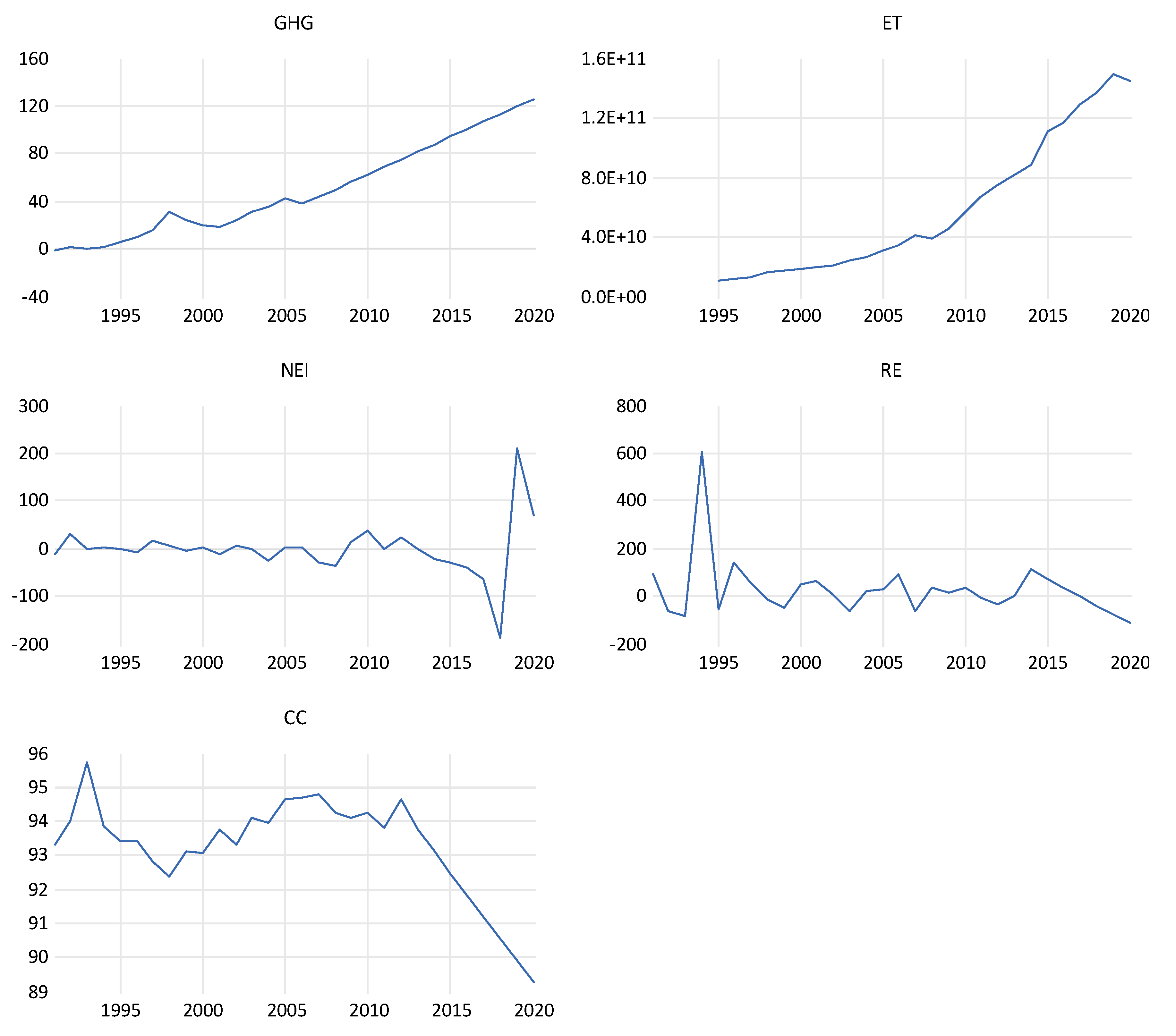
• Greenhouse Gas Emissions (GHG): Quantified in kilotons of CO₂-equivalent, the original data were sourced from the World Bank database. No changes were made to maintain clarity in levels.
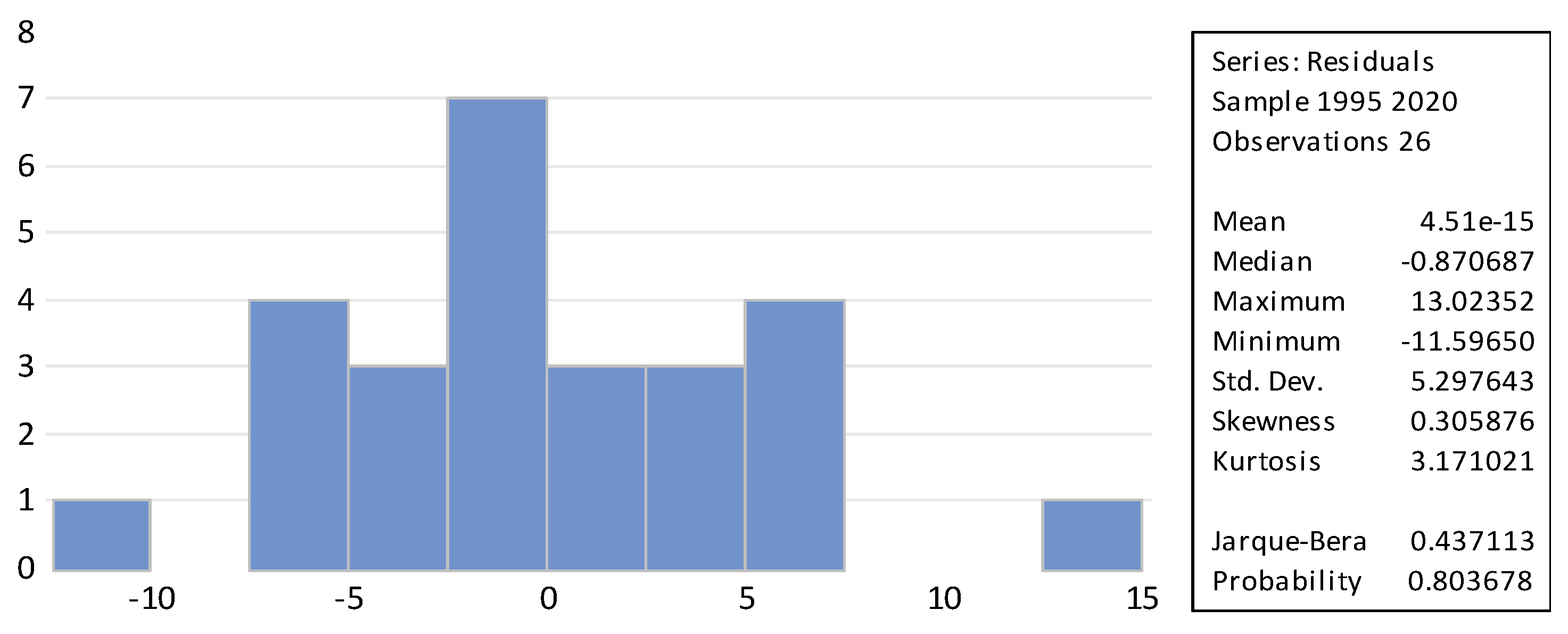
• Environmental Tax Revenue (ET): This variable reflects the overall tax income generated from environmental tax tools, stated in nominal South African rand. Because of the existence of zero and near-zero values in the initial years of the sample (1995–1999), logarithmic transformation was not utilized. Utilizing log transformations in these instances would require incorporating arbitrary constants (e.g., log (ET + 1)), potentially skewing estimation outcomes and affecting economic interpretability [38]. According to the descriptive statistics (Section 4.2), the ET series exhibits positive skewness (skewness = 0.7485), indicating a lengthy right tail frequently seen in fiscal and revenue-related metrics. Although ARDL estimation is typically resilient to non-normal regressors, we recognize the possible effects on finite-sample inference and tackle this by conducting post-estimation residual diagnostics. Specifically, Jarque–Bera tests for normality on the model residuals validate normality (p = 0.8037), confirming that the skewness of the regressor does not affect the reliability of the t-statistics or F-tests applied in inference.
• Net Energy Import (NEI): Defined as the gap between energy imports and exports, NEI measures South Africa’s reliance on foreign energy sources. A favorable NEI signifies being a net energy importer, showing a dependence on external fuel sources. This variable holds theoretical significance as it reflects the indirect influence of energy trade on emissions via fuel mix composition, energy pricing, and technological spillovers. Although greater imports of cleaner fuels might lower emissions, dependence on imported fossil fuels or inefficiencies in energy conversion methods could worsen emissions. Therefore, the anticipated sign is theoretically unclear and reliant on context. Due to the existence of negative values (indicating net exports in specific years), log transformation was not possible; the series was kept in its original form and differenced according to stationarity results.
• Renewable Energy Consumption (RE): This variable measures the overall yearly usage of renewable energy (in GWh), including sources like solar, wind, hydroelectric, biomass, and geothermal energy. It was obtained from the World Bank’s World Development Indicators and indicates total renewable energy deployment instead of its proportional share. Due to its non-stationary characteristics in level form and in line with ARDL model prerequisites, the RE variable underwent a transformation through first differencing, thus quantifying the variation in renewable energy consumption from one year to the next. This differencing resulted in the appearance of both positive and negative values, which align conceptually with yearly rises and falls in renewable energy adoption.
• Coal Consumption (CC): Expressed in million tonnes of oil equivalent (Mtoe), these data were utilized in its original form without alteration, due to the fairly consistent variance. The normality of the distribution was evaluated, and first differencing was conducted as required based on the results of unit root tests.

All data series were yearly and spanned the period from 1995 to 2020. Missing values were examined and handled using linear interpolation in instances where there was just a one-year gap. To preserve data accuracy, gaps spanning multiple years were eliminated. Stationarity was evaluated through the Augmented Dickey-Fuller and Phillips-Perron tests, and the orders of integration were verified prior to implementing the ARDL modelling framework.

3.2.2. Justification and Description of Variables

This study employs a collection of explanatory variables chosen for their theoretical and empirical significance in assessing greenhouse gas (GHG) emissions in the context of South Africa.

Table 1. Justification of variables.

Variable	Abbreviation	Description	Expected Sign	Units	Source
Greenhouse Gas Emissions	GHG	Total greenhouse gas emissions in kilotonnes of CO2 equivalent, encompassing anthropogenic CO2, CH4, N2O, and F-gases (HFCs, PFCs, and SF6), excluding short-cycle biomass burning.	Dependent	Kt CO2	World Bank
Environmental Tax Revenue	ETAX	Revenue from taxes where the base is a physical unit or proxy with a negative environmental impact (e.g., carbon content, fuel volume). It reflects fiscal instruments aimed at curbing pollution and incentivizing cleaner behavior.	Negative (–)	Local Currency Units	IMF (via OECD/UNEP databases)
Net Energy Imports	NEI	Net imports of energy (in oil equivalents) capture structural reliance on foreign energy sources, affecting emissions via energy mix, security, and pricing.	Negative (–)	% of energy use	World Bank
Renewable Energy Consumption	RE	Total renewable energy consumption in physical units (e.g., GWh), not as a share	Negative (–)	GWh or % points	World Bank
Coal Consumption	COAL	Total consumption of coal (primary and derived), including hard coal, lignite, and peat, used mainly in power generation. Coal is a major driver of carbon emissions due to its high carbon intensity.	Positive (+)	Million tonnes oil equivalent (Mtoe)	World Bank

Source: Author’s own compilation.

below illustrates the rationale for every variable incorporated in the ARDL model, detailing their theoretical foundation, expected directional influence on GHG emissions, measurement units, and data origins.

Notes:

• Expected signs are based on theoretical literature and prior empirical studies. For example, environmental tax revenue is expected to have a negative relationship with emissions if taxes are effectively designed and revenues are reinvested in mitigation efforts [40,41].
• NEI is expected to exert a negative effect, assuming imports replace domestically produced carbon-intensive energy sources; however, effects may be ambiguous in the case of fossil fuel-dominated imports.

3.3. Estimation Strategy and Diagnostic Test

This study utilized the autoregression distributive lag modeling (ARDL) method to examine the impact of mitigation strategies—such as environmental taxes, renewable energy consumption, and coal consumption—on greenhouse gas emissions in South Africa. This model is selected because it allows for the simultaneous estimation of short-term and long-term relationships and is particularly suitable for time-series data with mixed order of integration (I(0) and I(1)) without requiring pre-testing for unit roots [38]. First and foremost, this method allows for the simultaneous estimation of short-term and long-term coefficients. Also, all variables are included in the model as endogenous. Additionally, there is no requirement to conduct pre-testing for the univariate features of the series. Despite the completion of pre-testing, the model is capable of estimating series that have a combination of orders of integration ranging from integrated of zero I(0) to first I(1) order, except for I(2). In addition, this method tackles the issue of endogeneity in the model because the causal link between the dependent and independent variables cannot be predetermined. Finally, this method is most appropriate for small sample sizes due to its superior properties for small samples compared to other techniques. This method is appropriate for examining the connection between economic growth and banking sector growth, and its utilization in research has been growing. The results and in-depth analysis of the study will shape the recommendations. The ARDL model is the most appropriate econometric technique for analyzing the effectiveness of mitigation policies on GHG emissions in South Africa. By applying ARDL, this study generates more reliable and policy-relevant insights into the relationship between energy efficiency, emissions reduction, and economic growth.

The model is expressed as follows:

Mathematical form

GHG = F(ET, NEI, RE, CC)

(1)

Econometric form

GHG_t = β₀ + β₁ET_t + β₂NEI_t + β₂RE_t + β₃CC_t + ε_t

(2)

3.3.1. Unit Root Tests

After gathering the data, the initial step involved examining the time series properties of the data to determine if the dataset is integrated. If there are signs of a unit root, the research will use the Augmented Dickey–Fuller (ADF) and Phillips–Perron (PP) unit root tests, as performed in ref. [42], to confirm data stationarity and reliability of results. The null hypothesis for the ADF and PP tests suggests the series has a unit root, while the alternative hypothesis suggests the data are stationary either at level or after taking the first difference. This measure is taken to make sure that none of the variables are of order two or higher.

3.3.2. Optimal Lag Selection

Choosing the right lag is key in time series analysis, as it affects how well time series models perform, how easy they are to understand, and how efficiently they run. The ARDL bound testing method for establishing long-term relationships between variables requires selecting the optimal lag for the cointegrating equation, assuming no correlation among residuals [43]. Different lag lengths can be chosen to make adjustments in the model and achieve well-behaved residuals. Ref. [44] suggests that Akaike information criteria and Final Prediction Error are more effective for datasets with fewer than 60 observations. Due to the limited number of observations, lag selection in this study will be determined using Akaike information criteria and Final Prediction Error.

3.3.3. Bounds Test

Ref. [45] suggests that the ARDL bounds test is a useful approach for analyzing cointegration. The ARDL cointegration method is now widely recognized as a highly efficient approach to determining the parametric equation of the series within the Error Correction Model and confirming the existence of a long-term relationship between non-stationary time series variables. The null hypothesis suggests there is no cointegration, while the alternative hypothesis suggests there is cointegration [42]. If there is cointegration, it means that we can estimate long-term and short-term coefficients by using an error correction model without restrictions, as shown below.

ΔGHG_t = α₀ + α₁GHG_t−1 + α₂ET_t−1 + α₃NEI_t−1 + α₄RE_t−1 + α₅CC_t−1 + ∑β₁ΔGHG_t−1 + ∑β₂ΔET_t−1 + ∑β₃ΔNEI_t−1 + ∑β₄ΔRE_t−1 + ∑β₅ΔCC_t−1 + ε_t

(3)

where α₁–α₅ are estimated long-run coefficients and β₁–β₅ are estimated short-run coefficients. The tests are designed to discover the presence of a long-run association between variables using an F-test statistic. This is accomplished by comparing the estimated value to the crucial values to make a choice concerning the cointegration hypothesis. The resulting F-test statistics are compared to the two crucial boundaries, the lower and upper bounds, to determine cointegration. If the estimated value is more than the upper critical constraint, the null hypothesis of no cointegration can be rejected.

3.3.4. Estimating Short-Run Coefficients

After performing the cointegration test and discovering its presence, it advises estimating an error correction model. This contributes to determining the rate at which the variables adapt to their long-run equilibrium value [38]. The error correction model can be stated as follows:

$$∆{GHG}_t={\alpha }_0+{\sum }_{i=1}^P{\alpha }_1∆{GHG}_{t-1}{\sum }_{i=1}^P{\alpha }_2∆{ET}_{t-1}+{\sum }_{i=1}^P{\alpha }_3∆{NEI}_{t-1}{\sum }_{i=1}^P{\alpha }_4∆{RE}_{t-1}{\sum }_{i=1}^P{\alpha }_5∆{CC}_{t-1}+\phi {ECM}_{t-1}+{\epsilon }_t$$

(4)

ECM is a residual from the estimated cointegration Equation (3) and is the quantity that indicates the long-run adjustment speed. The ECM coefficient should ideally have a negative sign, be statistically significant, and be smaller than unity.

3.3.5. Research Reliability and Validity

This research relies on secondary data obtained from two respected organizations: the World Bank and the International Monetary Fund (IMF). Both groups are well known for their thorough databases and strict methods, guaranteeing the accuracy and authenticity of their information. The World Bank provides thorough information on worldwide economic measures, progress criteria, and financial data, carefully gathered and evaluated to assist in international economic evaluations and policy formation. In the same way, the IMF provides a vast amount of data on macroeconomic stability, financial stability, and global economic trends, utilizing various economic models and empirical research.

The World Bank and IMF use strong data gathering and verification methods, such as peer reviews and methodological audits, to uphold the precision and uniformity of their data. Their strong research facilities and dedication to openness also boost the credibility of the information they generate. Therefore, the information gathered from these organizations is seen as very trustworthy and legitimate for guiding this research, guaranteeing that the examination and findings made are rooted in strong and believable economic data.

3.3.6. Post-Test/Diagnostics

• Normality Test

Normality tests assess whether a dataset follows a normal distribution, with the null hypothesis stating that residuals are normally distributed. The Jarque–Bera test is commonly used, and a p-value below 0.01 leads to the rejection of normality at the 10% significance level. Meeting the normality assumption is essential to ensure valid results. If violated, a stationarity test is required to examine other characteristics of the data series. The following is the Jarque–Bera model:

$$JB={\displaystyle \frac{n}{6}} (s^2+{\displaystyle \frac{1}{4}} (k-2{)}^2)$$

(5)

where n is the sample size and JB is the Jarque–Bera statistic. Kurtosis is referred to as k, while skewness is referred to as s. The Jarque–Bera test precisely compares the data’s skewness and kurtosis to determine if it corresponds to a normal distribution [46].

• Multicollinearity

Multicollinearity is a statistical phenomenon in which two or more predictor variables in a multiple regression model are highly correlated, making it difficult to isolate the individual effect of each variable on the dependent variable. When predictor variables are uncorrelated, they are referred to as orthogonal. High intercorrelations among independent variables can lead to inflated standard errors and unreliable coefficient estimates, potentially skewing the interpretation of regression results. Despite this, we argue that in cases of imperfect multicollinearity, it remains possible to obtain Ordinary Least Squares (OLS) estimates that are Best Linear Unbiased Estimators (BLUE). The hypothesis test for multicollinearity posits a null hypothesis of no multicollinearity against the alternative that multicollinearity exists within the model [46].

• Heteroskedasticity

Heteroskedasticity represents a violation of the classical assumptions of linear regression and can compromise the validity of econometric analysis. However, if the model is correctly specified and the explanatory variables are uncorrelated with the error term, the Ordinary Least Squares (OLS) estimators remain unbiased and consistent despite the presence of heteroskedasticity [47]. The null hypothesis in testing for heteroskedasticity states that the error terms have constant variance, while the alternative suggests the presence of heteroskedasticity [48].

• Serial Correlation

Autocorrelation refers to the correlation of a time series with its own past values. In linear regression, the assumption is that residuals are not autocorrelated. The null hypothesis states there is no autocorrelation, while the alternative suggests its presence. The Breusch–Godfrey test is commonly employed to detect serial correlation in residuals, particularly of higher orders, making it a reliable diagnostic tool [48].

• Ramsey Test

The Ramsey test is used to assess the stability, validity, and effectiveness of autoregressive (AR) models over time. A model is considered stable if all unit roots have absolute values less than one and lie within the unit circle. To further test stability, the method developed by authors [49] employs recursive residuals, making it suitable for detecting structural changes in time-series data. The null hypothesis assumes constant coefficients, while the alternative suggests a varying coefficient vector.

• Stability Test

The stability test assesses whether an autoregressive (AR) model remains consistent over time in terms of efficiency, validity, and applicability. A model is considered stable if all variables have absolute values less than one and lie within the unit circle. Ref. [50], which analyzes standardized residuals, is particularly effective for detecting structural changes in time-series data. While the null hypothesis assumes constant coefficients over time, the alternative suggests variability in the coefficient vector.

3.4. Model Assumptions and Limitations

The econometric analysis in this study utilizes time-series data from South Africa, using models like the Autoregressive Distributed Lag (ARDL) framework to evaluate the connection between mitigation policies and GHG emissions. The ARDL methodology is based on several important assumptions, which include the stationarity of variables in their levels or first differences (i.e., I (0) or I (1)), the lack of I (2) series, and the presence of a long-run cointegrating relationship among the chosen variables.

Although the ARDL method is appropriate for small sample sizes and provides reliable long-run estimates with varying integration orders, some limitations should be recognized. Initially, limited samples can reduce the statistical strength of the model and increase the risk of type II errors, possibly masking meaningful connections. Furthermore, brief durations might restrict the applicability of results and hinder the reliability of diagnostic evaluations.

Secondly, while the ARDL bounds testing method considers endogeneity in the short term by including lagged dependent and independent variables, it does not completely resolve the possibility of structural endogeneity due to omitted variables, measurement inaccuracies, or reverse causation. This is especially important when examining policy measures such as carbon taxation, which could be simultaneously influenced by economic and environmental results.

Third, limitations in data, specifically the absence of high-frequency, detailed data on low-carbon technology imports and emissions by sector, can impact the accuracy of coefficient estimates and the understanding of policy effectiveness. Furthermore, unobserved structural changes, like shifts in policy regimes or global commodity price fluctuations, can lead to instability in parameter estimates as time progresses.

Nonetheless, despite these constraints, the study employs stringent diagnostic testing methods (e.g., serial correlation, heteroskedasticity, and model stability valuations) to improve the reliability of the estimated findings. The results must still be viewed carefully, recognizing the limitations set by data accessibility and the structural intricacies present in the South African situation.

4. Findings and Discussion

4.1. Descriptive Statistics

Table 2. Descriptive statistics.

Statistic	GHG	ET	NEI	RE	CC
Mean	57.1000	5.88 × 1010	−3.2512	9.7349	93.0960
Median	46.9545	4.00 × 1010	−1.3725	13.8956	93.4070
Maximum	125.9758	1.49 × 1011	211.8577	142.2365	94.7701
Minimum	6.3425	1.09 × 1010	−189.3993	−115.3336	89.2494
Std. Dev.	36.8137	4.64 × 1010	62.5476	61.6073	1.4847
Skewness	0.4212	0.7485	0.5954	0.0767	−1.1647
Kurtosis	1.8876	2.1235	9.2140	2.5906	3.5695
Jarque–Bera	2.1093	3.2600	43.3677	0.2071	6.2302
Probability	0.3483	0.1959	0.0000	0.9016	0.0444
Sum	1484.599	1.53 × 1012	−84.5303	253.1077	2420.495
Sum Sq. Dev.	33,881.29	5.39 × 1022	97,805.06	94,886.46	55.10883
Observations	26	26	26	26	26

Source: Author’s own computation using EViews 14.

provides a summary of the statistical results. A series with a kurtosis of three, a skewness of zero, and a Jarque–Bera p-value above a 5% significance level is normally distributed.

Greenhouse Gas Emissions (GHG): The mean GHG emissions stand at 57.1 units, indicating a substantial average level of emissions. The median value of 46.9545 suggests a slightly skewed distribution towards higher values, corroborated by the positive skewness of 0.4212. The range of emissions is vast, with a minimum of 6.3425 and a maximum of 125.9758, reflecting significant variability (Std. Dev. of 36.8137). The kurtosis of 1.8876 indicates a distribution with thinner tails than a normal distribution. The Jarque–Bera statistic of 2.1093 and its corresponding probability of 0.3483 imply that the null hypothesis of normality cannot be rejected, suggesting a reasonably symmetric distribution of GHG emissions.

Environmental Tax (ET): Environmental Tax Revenue (ET): The average ET is 5.88 × 10¹⁰, and the median is 4.00 × 10¹⁰, which suggests a positively skewed distribution (skewness = 0.7485). This right-skewness aligns with fiscal series in which revenues usually increase over time and are responsive to structural reforms. Despite the absence of log transformation on the data because of zero values in the early year, the distributional implications were thoroughly assessed through residual diagnostics after estimation, ensuring that the non-normality in the ET regressors did not skew model inference.

Net Energy Imports (NEI): The NEI variable shows an average of −3.2512 and a median of −1.3725, indicating that South Africa is generally a net energy exporter throughout the sample period. The series shows significant variability, with values between −189.3993 and 211.8577 and a standard deviation of 62.5476. The distribution reveals a slight right skew (skewness = 0.5954), while the kurtosis of 9.2140 indicates a significant leptokurtic distribution, suggesting the presence of frequent extreme values. The Jarque–Bera statistic of 43.3677 (p = 0.0000) decisively refutes the null hypothesis of normality. Even though ARDL estimation does not necessitate normal distribution [38], having high kurtosis can heighten susceptibility to outliers and make coefficient interpretation more complex.

Renewable Energy Consumption (RE): The RE variable, representing first-differenced values of renewable energy usage in GWh, shows a mean of 9.73 and a median of 13.90. The span varies between −115.33 and 142.24, aligning with phases of growth and decline in renewable energy adoption. The standard deviation is 61.61, reflecting considerable variability between years. Even though the Jarque–Bera statistic (0.2071) indicates near-normality, this should be interpreted carefully since differenced energy data may resemble normality but not completely adhere to normality assumptions.

Coal Consumption (CC): The variable shows minimal dispersion, evidenced by the small range between the minimum (89.2494) and maximum (94.7701), along with a standard deviation of 1.4847. The distribution exhibits a moderate left skew (skewness = −1.1647) and has a kurtosis of 3.5695, indicating somewhat heavier tails compared to the normal distribution. The Jarque–Bera statistic of 6.2302 (p = 0.0444) shows a statistically significant departure from normality at the 5% threshold. Although this does not breach the assumptions of the ARDL framework, extreme distributional characteristics can influence inference efficiency and should be interpreted with care.

4.2. Preliminary Tests

4.2.1. A Stationarity Test

• Visual Inspection

Figure 1 reveals that the variables NEI and RE are stationary at level form while the variables GHG, ET AND CC are non-stationary at level form.

4.2.2. Expanded Presentation of Unit Root Tests

Testing for unit root is necessary in ARDL analysis to ensure that the series are not integrated beyond order one. Therefore, employing an ARDL method with data that have a level of integration higher than one could result in misleading outcomes. The outcomes from

Table 3. ADF and PP.

Variable	Model Specification	ADF		PP		Order of Integration
		Levels	First Difference	Levels	First Difference
GHG	Intercept and trend	0.0148 ***	0.3033	0.9158	0.0000 ***	1
	Intercept	0.9998	0.0006 ***	1.0000	0.0006 ***	1
ET	Intercept and trend	0.8232	0.0056 ***	0.8254	0.0056 ***	1
	Intercept	0.9997	0.0140 ***	0.9997	0.0120 ***	1
NEI	Intercept and trend	0.0000 ***	0.0000 ***	0.0000 ***	0.0000 ***	1 and 0
	Intercept	0.0000 ***	0.0000 ***	0.0000 ***	0.0000 ***	1 and 0
RE	Intercept and trend	0.0000 ***	0.0000 ***	0.0000 ***	0.0001 ***	1 and 0
	Intercept	0.0000 ***	0.0000 ***	0.0000 ***	0.0001 ***	1 and 0
CC	Intercept and trend	0.9886	0.0002 ***	0.9654	0.0002 ***	1
	Intercept	0.9688	0.0021 ***	0.9759	0.0001 ***	1

*** Means the rejection of null hypothesis at all critical levels, i.e., 1%, 5%, and 10%; Source: Author’s own computation using EViews 14.

demonstrate that all variables are found to be stationary either in their original form or after undergoing a first difference, based on the ADF and PP unit root tests. This means that the data are appropriate for conducting an ARDL regression analysis, and the unit root null hypothesis can be dismissed at one percent and five percent significance levels.

Interpretation

The ADF and PP tests indicate that the dataset comprises both I(0) and I(1) series, yet no variable is integrated at the second order. In particular, NEI and RE are level stationary, whereas GHG, ET, and CC become stationary following first differencing. This confirms the suitability of the ARDL bounds testing method, as it allows for mixed integration orders while maintaining the model’s fundamental assumptions.

4.3. Determination of Optimal Lag Length

After determining the individual features of the variables and their sequence of integration, the next step is to choose the most suitable lag length for the model. The lag length criterion, including the Akaike information criterion (AIC), Schwarz Bayesian criterion (SC), and Hannan–Quinn criterion (HQ), was employed to determine this. This study chose to adhere to the SC and HQ information criteria due to their robustness and reliability.

Table 4. Lag selection criterion.

Lags	LogL	LR	FPE	AIC	SC	HQ
0	−1032.191	NA	7.47 × 1029	82.9753	83.21908 *	83.04291
1	−929.4702	156.1359 *	1.56 × 1027 *	76.75762 *	78.22027 *	77.16330 *

* indicates lag order selected by the criterion; LR: Sequential modified LR test statistics (each test at 5% level); FPE: Final Prediction Error; AIC: Akaike information criterion; SC: Schwarz information criterion; HQ: Hannan–Quinn information criterion. Source: Author’s own computation using EViews 14.

below reports that the two criteria indicated a lag length of one.

• Interpretation and Justification

The optimal lag order of 1 was chosen due to the lowest AIC and FPE values, which are suitable considering the small sample size (n = 26). According to the author of [40], AIC often surpasses other criteria in cases of small samples. Lag order 1 prevents overfitting and preserves degrees of freedom for accurate inference.

4.4. ARDL Bounds Testing Result

4.4.1. ARDL Bounds Testing Result

The ARDL bounds testing method verifies the presence of a statistically meaningful long-term equilibrium relationship between greenhouse gas (GHG) emissions and the identified explanatory factors: environmental taxes (ET), net energy imports (NEI), renewable energy consumption utilization (RE), and coal usage (CC). The F-statistic of 4.6636 exceeds the upper bound critical value at the 1% significance level (I (1) = 4.37), leading to a strong rejection of the null hypothesis of no cointegration (

Table 5. ARDL cointegration bounds test.

Test Statistic	Value	Signif.	I(0)	I(1)
F-statistic	4.6636	10%	2.2	3.09
K	4	5%	2.56	3.49
		2.5%	2.88	3.87
		1%	3.29	4.37

Source: Author’s own computation using EViews 14.

). This finding validates the following analyses of long-run and short-run dynamics through the ARDL error correction representation, providing empirical backing for the basic theoretical model that suggests a continuous connection among fiscal, energy, and environmental indicators.

Considering the presence of a sustained connection between GHG and the variables in the model, the research proceeds to calculate the long-term and short-term ARDL error correction equations. The outcomes are displayed in

Table 6. Long-run estimates using the ARDL.

Dependent Variable: GHG
Included Observations: 26
Long-Run Coefficients Using the ARDL
Variable	Coefficient	Std. Error	t-Statistic	Prob.
ET	9.01 × 10−10	1.04 × 10−10	8.6749	0.0000
NEI	0.0089	0.0502	0.1776	0.8609
RE	−0.0722	0.0711	−1.0146	0.3230
CC	6.6656	3.9499	1.6875	0.1079
C	−605.6720	367.2469	−1.6492	0.1155

Source: Author’s own computation using EViews 14.

.

4.4.2. Long-Run Estimates

• Long-Run Interpretation

• Environmental Taxes (ETs)

The long-run results of the ARDL model offer essential understanding of the structural factors influencing greenhouse gas (GHG) emissions in South Africa. The coefficient for ET is not only positive but also significantly substantial (p < 0.01), indicating that, surprisingly, rising environmental taxes correlate with increased GHG emissions over the long term. Although this outcome contradicts typical Pigouvian assumptions, it aligns with the empirical evidence presented by the author of [16], who links comparable anomalies in BRICS economies to the fiscal characteristics of environmental tax systems, where revenues are not consistently allocated for green investment or emissions reduction. In the South African setting, this result highlights the mismatch between the goals of environmental taxation and the real distribution methods. In theory, this reinforces the claim by the author of [48], which states that the effectiveness of environmental taxes depends not just on their implementation but also on the institutional framework that supports their usage.

• Net Energy Imports (NEIs)

The coefficient for net energy imports (NEIs) of 0.0089, along with a high probability value of 0.8609, suggests that NEI has a minor influence on GHG emissions. This indicates that fluctuations in net energy imports do not significantly impact emissions in South Africa. This outcome suggests that the dynamics of energy exchange, whether via heightened imports or diminished export actions, do not significantly affect the nation’s emissions path. This finding highlights a broader methodological issue: trade-oriented energy variables like NEI might not adequately represent the domestic structural factors influencing emissions, like sectoral energy intensity, fuel mix composition, and energy efficiency on the production side. The insignificance of NEI corresponds with the issues highlighted by the authors of [15], who stress that the success of energy-related policy tools depends on a nation’s unique economic framework and environmental starting points. For South Africa, a reliance on coal for energy and significant industrial energy intensity indicate that net energy trade dynamics, often influenced by global market changes, are a less critical factor in determining local emission results. This highlights the necessity for detailed, sector-specific indicators like electricity generation by fuel type, industrial energy usage, and transport energy requirements, which could better reflect localized emissions patterns.

• Renewable Energy Consumption (RE)

The coefficient on REC (−0.0722), even though statistically insignificant (p = 0.3230), has the theoretically expected sign: annual increases in renewable energy consumption are associated with reductions in GHG emissions. This result, however, highlights that short-run variability in renewable energy deployment may not yet exert a stable long-run influence on emission trajectories in South Africa. This finding is aligned with prior empirical evidence by refs. [21,49], which emphasizes that the scale and consistency of renewable energy investment must reach a threshold before producing measurable emission reductions in carbon-intensive economies.

• Coal Consumption (CC)

CC, featuring a significant positive coefficient (6.6656) and a p-value nearing marginal significance (p = 0.1079), underscores the meaningful long-term impact of coal consumption on GHG emissions. The size of the coefficient indicates a significant elasticity of emissions concerning coal consumption, highlighting the essential part of coal in South Africa’s carbon-heavy development trajectory. This outcome supports the findings of refs. [27,28], who record the persistent connection between coal reliance and elevated emissions in developing countries. The implication is that strategies for decarbonization should focus on structural changes away from coal by means of regulatory limits, renewable energy incentives, and fair transition measures for communities dependent on coal.

• Short-Run Coefficients (Table 7)

Table 7. Short-run coefficients using the ARDL.

Dependent Variable: GHG
Included Observations: 26
ECM Short-Run Dynamic ARDL Estimation
Variable	Coefficient	Std. Error	t-Statistic	Prob.
D(CC) (coal consumption)	−1.7301	1.4998	−1.4998	0.2630
CointEq (−1)	−0.2799	0.0471	−5.9452	0.0000

Source: Author’s own computation using EViews 14.

Table 7. Short-run coefficients using the ARDL.

Dependent Variable: GHG
Included Observations: 26
ECM Short-Run Dynamic ARDL Estimation
Variable	Coefficient	Std. Error	t-Statistic	Prob.
D(CC) (coal consumption)	−1.7301	1.4998	−1.4998	0.2630
CointEq (−1)	−0.2799	0.0471	−5.9452	0.0000

Source: Author’s own computation using EViews 14.

• Short-Run Estimates

Table 7 presents the short run, the estimated model using the ARDL approach reveals significant insights into the relationship between coal consumption and greenhouse gas (GHG) emissions in South Africa.

• Coal Usage (Short-run)

In the short-run analysis of the ARDL model, coal usage (D (CC)) shows a negative coefficient of −1.7301; nonetheless, this finding is not statistically significant at the 5% threshold (p = 0.2630). Per standard econometric interpretation, such insignificance suggests that the model fails to demonstrate a short-run link between coal consumption and greenhouse gas emissions [35]. As a result, no inferential claims are presented concerning the causal effect or directional trend of coal consumption in the short term. Although sectoral factors or operational delays may affect short-term emissions responses, this study does not empirically investigate these mechanisms, and therefore they are not examined further. Future studies might explore these dynamics by utilizing higher-frequency or sector-specific data or by employing non-linear time-series models.

• Error CorrectionTerm (ECT)

The coefficient for the error correction term (CointEq (−1)) is −0.2799 and shows statistical significance at the 1% level (p < 0.01). This suggests that around 28% of the difference from the long-term balance in GHG emissions is adjusted annually. The significant and negative sign of the ECT affirms the existence of a stable long-term relationship and suggests that the system demonstrates convergence to equilibrium following short-term disturbances. This reinforces the dynamic consistency of the ARDL model as described by ref. [14], thus confirming the structural characteristics of the model.

4.5. Post-Test Results (Diagnostic Tests)

• NormalityTest (Jarque–Bera Test and Figure 2)

A Jarque–Bera test was run on the model’s residuals to assess the inference’s dependability in the presence of skewed regressors, particularly Environmental Tax Revenue (ET). The test yielded a p-value of 0.8037, indicating that the residuals are distributed normally. This finding confirms that the consistency of the regression disturbance terms is maintained despite the non-normal distribution of some explanatory variables. Therefore, within the bounds of conventional inference, parameter estimates and the hypothesis tests that go along with them remain legitimate. Figure 2, which shows that the residuals closely match a normal distribution with a skewness of 0.31 and a kurtosis of 3.17, further supports these conclusions.

Figure 2. Normality. Source: Author’s own computation using EViews 14.

Figure 2. Normality. Source: Author’s own computation using EViews 14.

• Heteroskedasticity (Breusch–Pagan–Godfrey Test)

The Breusch–Pagan test result reports a p-value of 0.2950, indicating that the null hypothesis of homoskedastic residuals cannot be rejected (

Table 8. Diagnostic Results.

Normality Test
If the p-value is below 0.05, we reject the null hypothesis, which assumes that the residuals are normally distributed in normality testing. In this model, the probability of 0.80 exceeds the significance level of 0.05, leading us to not reject the null hypothesis.
Multicollinearity
Variable	Centered VIF
ET	2.1494
NEI	1.0630
RE	1.2068
CC	2.2746
The null hypothesis is rejected since all values under VIF are less than 5; therefore, there is no multicollinearity.
Heteroskedasticity
F-statistic	1.2272	Prob. F(4.38)	0.3294
Obs. * R-square	4.9260	Prob. Chi-square (4)	0.2950
Scaled explained SS	3.4884	Prob. Chi-square (4)	0.4797
Therefore, since the chi-square probability is 0.2950, which exceeds the 0.05 significance level, the null hypothesis cannot be refuted, indicating that the variances in the model remain consistent. Note: Asterisks in the regression tables denote statistical significance levels at p < 0.1 (), p < 0.05 (), and p < 0.01 (), respectively.
Serial Correlation
F-statistic	Durbin–Watson statistic	Observed R-Squared	Prob. chi-square
0.8846	1.5	0.2.2147	0.3304
In this case, the R-square p-value of 0.3304 exceeds the 5 percent significance level, indicating that the null hypothesis of no autocorrelation cannot be disproved.
Stability Test
The CUSUM test is applied to check the stability of the estimated parameters of the model. The result from the CUSUM reveals that the estimated lines are within the critical limits of the 5% level of significance. Therefore, it is confirmed that the variables of the estimated model remained stable during the sample period of the study.

Source: Author’s own EViews 14 computations.

). Thus, there is no statistical evidence of heteroskedasticity, and the variance of the error terms remains constant across observations.

• Serial Correlation (Breusch–Godfrey LM Test)

The p-value of 0.3304 from the Breusch–Godfrey test suggests no significant autocorrelation in the model’s residuals. This supports the ARDL assumption of uncorrelated error terms, which is essential for unbiased coefficient estimates and efficient inference.

• Multicollinearity(Variance Inflation Factor—VIF)

The VIF scores for all explanatory variables are below 2.3, well below the critical threshold of 5. This confirms that multicollinearity is not a concern in this model, and the estimated coefficients can be interpreted reliably without confounding interaction effects among independent variables.

• Specification Test (Ramsey RESET Test)

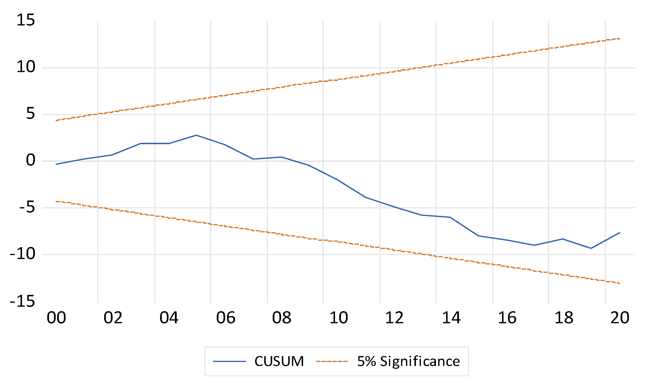
The RESET test yielded a p-value above 0.05, implying that the model is correctly specified. There is no evidence of omitted variable bias or incorrect functional form, suggesting the regression structure is appropriate for the data and theoretical framework.

• Stability Test (CUSUM Chart, Figure 3)

The CUSUM test confirms the stability of the estimated model parameters over the sample period. Figure 3 illustrates that the cumulative sum of residuals remains within the 5% significance bounds, indicating that there are no structural breaks or time-varying parameter instabilities. This is crucial for the reliability of long-run and short-run ARDL estimates.

Figure 3. CUSUM. Source: Author’s own computation using EViews 14.

Figure 3. CUSUM. Source: Author’s own computation using EViews 14.

• Validation of Models and Diagnostics for Robustness

Due to the constraints of the sample size, sub-sample analysis and alternative model specifications were not performed, as they would greatly diminish degrees of freedom. Instead, a thorough array of diagnostic tests following estimation was utilized. According to Table 8, the model meets essential assumptions of classical linear regression: residuals exhibit a normal distribution, are homoskedastic, and lack serial correlation; the functional form is accurately specified; multicollinearity is absent; and the CUSUM test verifies parameter stability. These diagnostics offer solid proof that the ARDL estimates are statistically dependable and sturdy, even with the limited sample size and non-normal input variables.

• Policy and Academic Implications

The findings of this study offer several policy-relevant insights. First, given the unexpectedly positive coefficient, which indicates that environmental taxes are ineffective at reducing emissions, immediate adjustments to fiscal policy tools are required. These include allocating revenues for climate projects, increasing the transparency of tax design, and coordinating emissions pricing with sector-specific decarbonization goals. Second, rather than relying on supply-side or overall trade indicators, a comprehensive, sector-oriented approach to emissions reduction is required, as seen by the importance of renewables and the little influence of NEI. Third, coal’s critical role underscores the need for a just energy transition model that protects vulnerable areas from economic disruption, ensures energy security, and reduces emissions.

From an academic perspective, this research enhances the growing body of literature on the effectiveness of environmental fiscal policies in middle-income, coal-reliant nations. It further confirms the effectiveness of the ARDL method in separating short-term fluctuations from long-term structural trends in emissions patterns. Future studies should include broader institutional factors like governance quality, funding for green R&D, and updates to the grid to better contextualize the causes of emissions in the Global South.

4.6. Conclusions

The dynamic and long-term factors impacting greenhouse gas (GHG) emissions in South Africa, a country grappling with the dual challenges of sustaining economic growth and addressing escalating environmental degradation, were extensively investigated in this study. The study focused on key explanatory variables, such as market-based instruments, particularly environmental tax revenues, and structural energy factors, such as the use of renewable energy, coal consumption, and net energy imports, using the Autoregressive Distributed Lag (ARDL) modeling framework. These factors were specifically selected to show how fiscal policy instruments relate to the basic energy consumption trends affecting the nation’s emissions trajectory.

Results from empirical research were unexpected yet significant. Important questions concerning the effectiveness and design of the existing environmental tax system are raised by the significant positive and statistically significant relationship between the long-term coefficient for environmental tax revenue and GHG emissions. This suggests that current tax systems may not sufficiently concentrate on or reinvest in methods to effectively promote emissions reduction, potentially even encouraging detrimental environmental behavior when revenue is not purposefully allocated to environmentally positive projects. Furthermore, the small and statistically negligible impact of using renewable energy on emissions emphasizes how little and how little renewable technologies are used in South Africa’s energy mix, demonstrating that the country is still in the early stages of its energy transition.

On the other hand, coal usage was confirmed as a strong and important contributor to emissions in both the short and long term, supporting South Africa’s deep-seated dependence on coal-fired electricity generation as a key component of its energy framework. This result is consistent with existing research on carbon-heavy emerging economies, highlighting the inherent structural difficulties in decarbonizing energy supply chains that are still largely reliant on fossil fuels.

The existence of an error correction term supports the model’s stability and the system’s ability to adapt to departures from long-term equilibrium relationships, thus strengthening the credibility of the derived policy implications. Together, these results highlight the need for cohesive policy frameworks that go beyond traditional fiscal measures and tackle structural interdependencies in the energy sector. The research enhances academic discussions by delivering strong empirical data relevant to an emerging economy with significant carbon emissions, identifying deficiencies in existing fiscal and energy frameworks, and establishing a basis for future studies on sustainable environmental management in similar developing country situations.

5. Summary of Key Findings and Policy Recommendation

5.1. Summary of Key Findings

• Environmental Taxation: An Incoherent Fiscal Instrument

The long-run ARDL findings reveal a statistically significant and positive relationship between environmental tax income and GHG emissions in South Africa. This challenges conventional assumptions about the emission-reducing function of environmental taxation. The findings indicate that existing fiscal tools could prioritize revenue generation over environmental goals, possibly due to ineffective enforcement, insufficient allocation of funds for green initiatives, or fragmented institutions. This corresponds with results in other BRICS nations (ref. [16]) where comparable structural inefficiencies weaken tax efficiency.

• Net Energy Imports: Slight Direct Effect

Net energy imports (NEI) show a statistically insignificant correlation with emissions. This implies that import dynamics by themselves cannot fully account for differences in GHG levels, likely due to the fact that the emissions effect of energy imports relies on the fuel composition, regulatory frameworks, and energy sector interconnectedness. Ref. [15] also observes that the effectiveness of energy import strategies in lowering emissions is largely contingent upon national structural and policy frameworks.

• Renewable Energy: Limited Emissions Effectiveness

Despite being theoretically predicted to lower emissions, the use of renewable energy in South Africa demonstrates no significant long-term effect on GHG emissions. This might indicate weak investment levels, inadequate infrastructure, or difficulties in integration. As noted by refs. [21,22], the success of renewables in developing areas frequently depends on strong institutional frameworks, grid capacity, and ongoing policy support—elements that are presently constrained in the South African scenario.

• Coal Usage: A Continuing Emissions Catalyst

Coal continues to be the largest source of long-run emissions, reinforcing South Africa’s reliance on carbon-heavy energy. This discovery supports the findings from refs. [27,28] and emphasizes the need for a unified strategy for phase-out that incorporates both regulatory measures and technological solutions to diversify the country’s energy mix.

• Short-Term Irrelevance, Long-Term Consistency

In the short run, coal consumption shows a statistically insignificant impact on emissions. The importance and direction of the error correction term verify the existence of a stable long-run equilibrium. This suggests that although immediate changes in policy may not produce instant results, the long-run emissions path is influenced by wider structural and financial factors.

5.2. Policy Recommendations

Policy Recommendations: Towards a Practical Low-Carbon Transition in South Africa.

Considering the empirical data that show the restricted impact of current environmental taxes and the ongoing reliance on coal, there is a need for a unified, practical policy structure. The subsequent suggestions are classified according to their implementation timeline and organizational viability.

• Short-Term Priorities (0–5 years)

• Adjustment of the Carbon Tax Structure

• Action: Remove exemptions for carbon-heavy industries and adjust the tax rate to match the marginal abatement cost.
• Institutional Responsibility: National Treasury and South African Revenue Service (SARS).
• Anticipated Effect: Enhance the price indication for lowering emissions and produce funds for eco-friendly investments.

• System for Monitoring Digital Emissions

• Initiative: Create a nationwide, real-time digital system for monitoring sector-specific GHG emissions.
• Institutional Accountability: Department of Forestry, Fisheries, and the Environment (DFFE), collaborating with CSIR.
• Anticipated Effect: Improve regulatory supervision and clarity in emissions reporting.

• Focused Green Industrial Benefits

• Action: Broaden incentive programs (e.g., Section 12L of the Income Tax Act) for local manufacturing of solar panels, electrolyzers, and grid parts.
• Institutional Accountability: Department of Trade, Industry and Competition (DTIC); Industrial Development Corporation (IDC).
• Anticipated Outcome: Boost local eco-friendly production and lessen reliance on technology imports.

• Coal Transition Area Investment Initiative

• Action: Initiate retraining programs and support funds for SMEs in Mpumalanga and other areas dependent on coal.
• Institutional Accountability: Department of Employment and Labour; Presidential Climate Commission.
• Anticipated Outcome: Alleviate workforce dislocation and encourage local economic variety.

• Measures for Long-Term Structure (5–15 years)

• Integrated Renewable Energy Implementation

• Action: Increase public–private investments in renewable energy via competitive auctions and power purchase agreements (PPAs), in accordance with the IRP.
• Institutional Responsibility: Department of Mineral Resources and Energy (DMRE); Eskom; Office of Independent Power Producers (IPPOs).
• Anticipated Outcome: Lower carbon emissions from electricity production and decrease Eskom’s carbon intensity.

• Grid Update and Connectivity

• Action: Enhance and broaden the national transmission network to facilitate decentralized renewable energy production.
• Institutional Accountability: Eskom Transmission Company; National Energy Regulator of South Africa (NERSA).
• Anticipated Effect: Mitigate transmission bottlenecks and enhance renewable grid integration.

• Formation of an Energy Transition and Climate Finance Agency

• Action: Organize concessional and blended financing for decarbonization, encompassing JET-IP alignment and global green bonds.
• Responsibility of Institutions: National Treasury; DBSA; Task Team for Presidential Climate Finance.
• Anticipated Outcome: Generate sustained investment for infrastructure related to mitigation and adaptation.

5.3. Limitations and Directions for Future Research

This study offers empirical insights into the factors influencing greenhouse gas emissions in South Africa but is constrained by various methodological and data-related limitations that require careful attention. Firstly, the analysis is limited by the existence of uniform annual data covering the period from 1995 to 2020, leading to a fairly small sample of 26 observations. Although the ARDL framework is recognized for its statistical robustness in small-sample contexts [38], constraints in degrees of freedom can reduce hypothesis testing power, elevate chances of Type II errors, and limit the model’s capacity to identify understated dynamic interactions. The suggestion is that certain relationships, especially those functioning through lag structures, might remain statistically unnoticed even though they hold theoretical significance. Future research might gain from utilizing quarterly data or other high-frequency indicators, potentially improving estimation accuracy and inference dependability.

Secondly, the ARDL model used in this context presumes linearity and consistent parameters throughout time. This prevents the identification of structural breaks that might occur due to significant policy changes, external shocks (such as the COVID-19 pandemic or global energy market disruptions), or shifts in institutional arrangements. Integrating break tests (such as Zivot–Andrews or Bai–Perron methods) or using time-varying parameter models might enhance the model’s sensitivity to past discontinuities.

Third, using aggregate-level variables, though suitable for identifying national trends, might mask significant differences across sectors. For instance, emissions from the industrial, residential, and transportation sectors might react differently to environmental taxes and the use of renewable energy. Upcoming studies might utilize detailed emissions data to investigate sector-specific trends and adjust policy measures accordingly.

Fourth, the assumption of linear functional forms could miss possible asymmetries or threshold effects in how environmental policy is transmitted. Future researchers might explore nonlinear models like Threshold ARDL or Smooth Transition ARDL to detect regime-dependent impacts, especially regarding the interplay between fiscal tools and energy transition strategies. Exploring the relationship between environmental tax revenues and fiscal redistribution mechanisms could be beneficial for evaluating the fairness and political viability of green tax reforms.

Finally, the strength of this study’s strategy is limited by the small sample size, which hindered the ability to conduct sub-sample regressions and test different model specifications. Nevertheless, comprehensive post-estimation diagnostics were performed to confirm model adequacy. Although these tests validate the dependability of parameter estimates and uphold the internal validity of the ARDL model, subsequent research should enhance this methodology with more sophisticated robustness techniques like quantile regressions or threshold models when longer or higher-frequency datasets are accessible.

In summary, South Africa’s shift to lower-carbon economic frameworks needs backing from both immediate regulatory actions and sustained fiscal, institutional, and technological approaches. These encompass a systematic coal phase-out strategy within the Just Energy Transition framework, enhanced coordination of environmental taxes, and focused public funding for renewable infrastructure.

References

1. Satgar, V. The climate crisis and systemic alternatives. In The Climate Crisis: South African and Global Democratic Eco-Socialist Alternatives; Wits University Press: Johannesburg, South Africa, 2018; pp. 1–28. [Google Scholar]
2. Sasu, D.D. Africa: CO2 Emissions by Country. 2024. Available online: https://www.statista.com/statistics/1268395/production-based-co2-emissions-in-africa-by-country/ (accessed on 10 March 2025).
3. Hanto, J.; Schroth, A.; Krawielicki, L.; Oei, P.Y.; Burton, J. South Africa’s energy transition–unraveling its political economy. Energy Sustain. Dev. 2022, 69, 164–178. [Google Scholar] [CrossRef]
4. South African Revenue Service. Carbon Tax. 2023. Available online: https://www.sars.gov.za/customs-and-excise/excise/environmental-levy-products/carbon-tax/ (accessed on 10 March 2025).
5. Vuzane, R. An Analysis of Carbon Tax and Other Environmental Levies: A South African and International Perspective. Master’s Dissertation, Rhodes University, Grahamstown, South Africa, 2020. [Google Scholar]
6. Errendal, S.; Ellis, J.; Jeudy-Hugo, S. The Role of Carbon Pricing in Transforming Pathways to Reach Net Zero Emissions: Insights from Current Experiences and Potential Application to Food Systems; OECD: Paris, France, 2023. [Google Scholar]
7. Nene, S.; Nagy, H. Legal regulations and policy barriers to development of renewable energy sources in South Africa. In Engineering for Rural Development, Proceedings of the International Scientific Conference (Latvia) (No. 20), Jelgava, Latvia, 26–28 May 2021; Latvia University of Life Sciences and Technologies: Jelgava, Latvia, 2021. [Google Scholar]
8. Ndlovu, V.; Inglesi-Lotz, R. The causal relationship between energy and economic growth through research and development (R&D): The case of BRICS and lessons for South Africa. Energy 2020, 199, 117428. [Google Scholar]
9. Adepeju, I.Z. Managing Climate Risks in Africa: Insights from South Africa and Ethiopia. Doctoral Dissertation, Memorial University of Newfoundland, St. John’s, NL, Canada, 2018. [Google Scholar]
10. IPCC (Intergovernmental Panel on Climate Change). Climate Change 2021: The Physical Science Basis; Contribution of Working Group I to the Sixth Assessment Report of the Intergovernmental Panel on Climate Change; Cambridge University Press: Cambridge, UK; New York, NY, USA, 2021. [Google Scholar]
11. Burke, M.J.; Stephens, J.C. Political power and renewable energy futures: A critical review. Energy Res. Soc. Sci. 2018, 35, 78–93. [Google Scholar] [CrossRef]
12. Smil, V. Energy in World History; Routledge: London, UK, 2019. [Google Scholar]
13. Jacobson, M.Z.; Delucchi, M.A.; Bauer, Z.A.; Goodman, S.C.; Chapman, W.E.; Cameron, M.A.; Yachanin, A.S. 100% clean and renewable wind, water, and sunlight all-sector energy roadmaps for 139 countries of the world. Joule 2017, 1, 108–121. [Google Scholar] [CrossRef]
14. Onofrei, M.; Vintilă, G.; Dascalu, E.D.; Roman, A.; Firtescu, B.N. The impact of environmental tax reform on greenhouse gas emissions: Empirical evidence from european countries. Environ. Eng. Manag. J. (EEMJ) 2017, 16, 2843–2849. [Google Scholar] [CrossRef]
15. Kotnik, Ž.; Maja, K.; Škulj, D. The effect of taxation on greenhouse gas emissions. Transylv. Rev. Adm. Sci. 2014, 10, 168–185. [Google Scholar]
16. Rybak, A.; Joostberens, J.; Manowska, A.; Pielot, J. The impact of environmental taxes on the level of greenhouse gas emissions in Poland and Sweden. Energies 2022, 15, 4465. [Google Scholar] [CrossRef]
17. Tang, Z.; Qin, D. Sustainable mining and the role of environmental regulations and incentive policies in BRICS. Resour. Policy 2024, 90, 104718. [Google Scholar] [CrossRef]
18. Sarfraz, M.; Ivascu, L.; Cioca, L.I. Environmental regulations and CO2 mitigation for sustainability: Panel data analysis (PMG, CCEMG) for BRICS nations. Sustainability 2021, 14, 72. [Google Scholar] [CrossRef]
19. Wisdom, O.; Apollos, N.; Samuel, O. Carbon accounting and economic development in sub-Saharan Africa. Asian J. Econ. Bus. Account. 2022, 22, 81–89. [Google Scholar] [CrossRef]
20. Wang, Y.K.; Zhang, X. Firm’s imperfect compliance and pollution emissions: Theory and evidence from South Africa. Asian J. Econ. Bus. Account. 2019, 1, 1–9. [Google Scholar] [CrossRef]
21. Verma, M.; Sati, M.; Uniyal, S. Impact of Renewable Energy in Reducing Greenhouse Gas Emissions. In Renewable Energy and Green Technology; CRC Press: Boca Raton, FL, USA, 2021; pp. 127–139. [Google Scholar]
22. Mandimby, A.S. Effect of Renewable Energi on CO2 Emissions in BRICS Countries. Quant. Econ. Manag. Stud. 2024, 5, 372–386. [Google Scholar] [CrossRef]
23. Riti, J.S.; Riti, M.K.J.; Oji-Okoro, I. Renewable energy consumption in sub-Saharan Africa (SSA): Implications on economic and environmental sustainability. Curr. Res. Environ. Sustain. 2022, 4, 100129. [Google Scholar] [CrossRef]
24. Kocak, E.; Ulug, E.E.; Oralhan, B. The impact of electricity from renewable and non-renewable sources on energy poverty and greenhouse gas emissions (GHGs): Empirical evidence and policy implications. Energy 2023, 272, 127125. [Google Scholar] [CrossRef]
25. Al-Ismail, F.S.; Alam, M.S.; Shafiullah, M.; Hossain, M.I.; Rahman, S.M. Impacts of renewable energy generation on greenhouse gas emissions in Saudi Arabia: A comprehensive review. Sustainability 2023, 15, 5069. [Google Scholar] [CrossRef]
26. Ziuku, S.; Meyer, E.L. Mitigating climate change through renewable energy and energy efficiency in the residential sector in South Africa. Int. J. Renew. Energy Technol. 2012, 2, 33–43. [Google Scholar]
27. Ayodele, T.R.; Munda, J.L. The potential role of green hydrogen production in the South Africa energy mix. J. Renew. Sustain. Energy 2019, 11, 044301. [Google Scholar] [CrossRef]
28. Malik, A.; Lan, J.; Lenzen, M. Trends in global greenhouse gas emissions from 1990 to 2010. Environ. Sci. Technol. 2016, 50, 4722–4730. [Google Scholar] [CrossRef]
29. Jiang, Q.; Rahman, Z.U.; Zhang, X.; Islam, M.S. An assessment of the effect of green innovation, income, and energy use on consumption-based CO2 emissions: Empirical evidence from emerging nations BRICS. J. Clean. Prod. 2022, 365, 132636. [Google Scholar] [CrossRef]
30. Guedie, R.; Ngnemadon, A.S.A.; Fotio, H.K.; Nembot, L. Disaggregated analysis of the effects of energy consumption on greenhouse gas emissions in Africa. Energy Econ. Lett. 2022, 9, 75–90. [Google Scholar] [CrossRef]
31. Saha, N.C.; Saha, D. Impact of coal mining on ambient air in respect of global warming: A critical approach. Indones. J. Soc. Environ. Issues (IJSEI) 2023, 4, 12–24. [Google Scholar] [CrossRef]
32. Wang, Q.; Song, X.; Liu, Y. China’s coal consumption in a globalizing world: Insights from Multi-Regional Input-Output and structural decomposition analysis. Sci. Total Environ. 2020, 711, 134790. [Google Scholar] [CrossRef] [PubMed]
33. Wen, J.; Yang, F.; Xu, Y. Coal consumption and carbon emission reductions in BRICS countries. PLoS ONE 2024, 19, e0300676. [Google Scholar] [CrossRef] [PubMed]
34. Adebayo, T.S.; Kirikkaleli, D.; Adeshola, I.; Oluwajana, D.; Akinsola, G.D.; Osemeahon, O.S. Coal consumption and environmental sustainability in South Africa: The role of financial development and globalization. Int. J. Renew. Energy Dev. 2021, 10, 527–536. [Google Scholar] [CrossRef]
35. Bekun, F.V.; Etokakpan, M.U.; Agboola, M.O.; Uzuner, G.; Wada, I. Modelling coal energy consumption and economic growth: Does asymmetry matter in the case of South Africa? Pol. J. Environ. Stud. 2023, 32, 2029–2042. [Google Scholar] [CrossRef]
36. Sadorsky, P. Trade and energy consumption in the Middle East. Energy Econ. 2011, 33, 739–749. [Google Scholar] [CrossRef]
37. Omri, A.; Nguyen, D.K. On the determinants of renewable energy consumption: International evidence. Energy 2014, 72, 554–560. [Google Scholar] [CrossRef]
38. Taghvaee, V.M.; Hajiani, P.; Aloo, A.S. Elasticities of Energy, Environment, and Economy in Long and Short Run: Using Simultaneous Equations, Error Correction and Cointegration Models. J. Emerg. Issues Econ. Financ. Bank. 2017, 6, 2155–2186. [Google Scholar]
39. Gujarati, D.N. Basic Econometrics, 4th ed.; Tata McGraw Hill: New York, NY, USA, 2002. [Google Scholar]
40. Ibeabuchi, I.J.; Amaefule, C.; Shoaga, A. Determinants of greenhouse gas emissions. Eur. J. Sustain. Dev. Res. 2022, 6, em0194. [Google Scholar]
41. Michel, B.; Falcao, T. OECD (2022) Public Consultation on Pillar One–Amount A: Draft Model Rules for Nexus and Revenue Sourcing: Comments by B. Michel and T. Falcao. Available online: https://papers.ssrn.com/sol3/papers.cfm?abstract_id=4266352 (accessed on 10 March 2025).
42. Aldy, J.E.; Stavins, R.N. Using the market to address climate change: Insights from theory & experience. Daedalus 2012, 141, 45–60. [Google Scholar]
43. Paavo, E. The Impact of Commercial Banks Development on Economic Growth in Namibia. Master’s Thesis, University of Cape Town, Cape Town, South Africa, 2018. [Google Scholar]
44. Yakubu, Y.; Salisu, B.M.; Umar, B. Electricity supply and manufacturing output in Nigeria: Autoregressive distributed lag (ARDL) Bound testing approach. J. Econ. Sustain. Dev. 2015, 6, 7–19. [Google Scholar]
45. Liew, V. On Autoregressive Order Selection Criteria. Master’s Thesis, Universiti Putra Malysia, Serdang, Malaysia, 2004. [Google Scholar]
46. Demirhan, H. dLagM: An R package for distributed lag models and ARDL bounds testing. PLoS ONE 2020, 15, e0228812. [Google Scholar] [CrossRef] [PubMed]
47. Asteriou, D.; Hall, S.G. Applied Econometrics; Bloomsbury Publishing: London, UK, 2021. [Google Scholar]
48. Ogujiuba, K.; Mngometulu, N. Does social investment influence poverty and economic growth in South Africa: A cointegration analysis? Economies 2022, 10, 226. [Google Scholar] [CrossRef]
49. Fullerton, D.; Metcalf, G.E. Tax Incidence; National Bureau of Economic: Cambridge, UK, 2001. [Google Scholar]
50. Woolridge, J.M. Introductory Econometrics: A Modern Approach; South Western Cengage Learning: Mason, OH, USA, 2009. [Google Scholar]
Figure 1. Graphical representation of all variables at level form. Source: Author’s own computation using EViews 14.
Sustainability 17 05531 g001