A Study on the Impact of the Digital Economy on the Industrial Collaborative Agglomeration of Manufacturing and Productive Service Industries

Abstract

The digital economy has profoundly reshaped industrial organizational structures and the spatial distribution of cooperative agglomerations in the manufacturing and productive service sectors. To support the coordinated and sustainable development of China’s industries, it is essential to clarify how the digital economy influences industrial cooperative agglomeration. This study first constructs a comprehensive index system capturing the quality, quantity, and synergy of industrial cooperative agglomeration, enabling an evaluation of collaborative agglomeration levels across 30 Chinese provinces. Second, the relationship between the digital economy and industrial collaborative agglomeration is examined using both static and dynamic spatial panel models. Finally, the paper investigates regional disparities in this relationship across eastern, central, and western China. The results reveal the following findings: (1) The digital economy has a significant inhibitory effect on industrial collaborative agglomeration overall. (2) Dynamic spatial lag model results show an inverted U-shaped relationship, where the digital economy initially promotes but later inhibits industrial agglomeration, with notable temporal lags and spatial spillover effects. (3) In eastern China, digital economy growth suppresses local agglomeration while promoting it in neighboring regions; in the central region, it enhances local agglomeration but dampens it in adjacent areas; and in the western region, the relationship is nonlinear and U-shaped.

1. Introduction

Since 2009, China has established a series of demonstration bases for new industrialization industries, promoting the collaborative concentration of manufacturing and productive service sectors through geographic clustering, resource sharing [1], and technological cross-fertilization [2,3]. These efforts have underscored the benefits of industrial clusters, enhanced industrial upgrading [4,5], and facilitated sustainable and high-quality industrial growth [6,7]. However, when industrial agglomeration reaches a certain threshold, several challenges emerge. First, the influx of labor leads to soaring land prices, traffic congestion, and pressure on educational resources. Second, excessive resource concentration generates environmental stress [8] and siphons resources from surrounding regions, resulting in unbalanced regional development. Third, over-agglomeration can trigger homogenized competition [9], weakening enterprises’ capacity to sustain technological innovation and R&D efforts.

Scholars have carried out extensive research on economic agglomeration. The majority of existing studies concentrate on the externalities of agglomeration, which are primarily reflected in the spillover effects of knowledge and technology generated by agglomeration and their influence on the economic development [10] and environmental conditions [11] of surrounding areas. Regarding the formation mechanism of industrial agglomeration, new economic geography posits that geographical location and historical advantages serve as foundational factors, while the increase in the number of enterprises and the generation of positive feedback mechanisms contribute to the amplification of agglomeration advantages [12]. Evolutionary economic geography highlights the critical roles of innovation and path dependence in shaping the agglomeration process [13]. Moreover, industrial and fiscal policies play a substantial role in influencing agglomeration patterns [14].

Research into the digital economy can be traced back to investigations of the platform economy, including topics such as platform-driven collaborative innovation and platform-based business models [15]. The digital economy has expedited the digital transformation of enterprises, thereby serving as a pivotal pathway for integrating the digital and real economies. Scholars have explored various dimensions of the digital economy, including the digital platform ecosystem, digital finance, technological innovation, and employment dynamics [16,17,18]. Additionally, the digital economy has the potential to reduce regional economic disparities [19], thus providing robust support for high-quality economic development [20]. The digital economy functions as a double-edged sword in influencing industrial agglomeration. On one hand, it facilitates the sharing of information, talent, and capital. Digital technologies reduce information asymmetry, lower acquisition costs, and enable rapid transfer of knowledge and technology across industries, thus promoting collaborative agglomeration [21]. The Internet fosters shared labor pools, while artificial intelligence compensates for labor shortages. Digital finance diversifies funding sources, assessing creditworthiness and repayment ability via big data and cloud computing to expedite lending and shorten financing cycles [22]. The high fluidity of data elements has significantly enhanced the efficiency of resource allocation, while digital technology has bolstered the collaborative innovation capabilities of enterprises [23]. Through improvements in production efficiency and the implementation of green technological innovations, enterprises have successfully achieved reductions in pollution and carbon emissions [24].

On the other hand, the digital economy can also inhibit industrial agglomeration through its diffusion effect. Technologies such as multimedia and virtual reality allow for the exchange of non-codable information, making cross-regional and inter-industry communication more convenient [25]. Some studies argue that the Internet eliminates geographic constraints, enabling firms to relocate from high-cost urban centers to lower-cost regions in response to land prices and environmental regulations, thereby contributing to industrial dispersion [26]. Additionally, the extensive infrastructure required for digital industry development consumes substantial energy, intensifying resource competition [27] and contributing to industrial fragmentation.

In summary, the digital economy exerts both agglomerative and dispersive effects on industrial clustering. Existing research primarily focuses on individual components of the digital economy. Studies show that network infrastructure [28], Internet development [29], and digital finance [30] promote collaborative agglomeration, while artificial intelligence demonstrates a U-shaped relationship with it [31]. However, there remains a lack of comprehensive research examining the overall influence of the digital economy on industrial collaborative agglomeration. Although some scholars argue that the digital economy promotes agglomeration [32,33], the relationship remains complex and possibly nonlinear. Thus, it is necessary to investigate not only whether the digital economy facilitates collaborative agglomeration but also whether its effects follow a linear trajectory.

Accordingly, this study examines the influence and spatial spillover effects of the digital economy on industrial collaborative agglomeration by constructing an improved index. It posits that the digital economy reshapes industrial clustering through mechanisms such as penetration, sharing, and spillover. Furthermore, it explores regional heterogeneity to provide a theoretical foundation for achieving coordinated and sustainable industrial development across different regions.

The main contributions of this study are as follows: (1) This paper introduces a coupling coordination degree model between manufacturing and productive service industries, based on the θ index, to construct a refined collaborative agglomeration index. This index comprehensively reflects the quality, quantity, and synergy of agglomeration, accounting for industry heterogeneity and addressing the limitations of existing synergy-based measures. (2) While most current studies emphasize the outcomes of industrial collaborative agglomeration, few examine the digital economy’s role in shaping it. This paper fills that gap and enriches the literature on the subject. (3) Methodologically, the study employs a dynamic spatial lag model to assess the relationship between the digital economy and industrial collaborative agglomeration, incorporating both temporal lags and spatial spillover effects. (4) The paper also investigates regional heterogeneity in this relationship, offering targeted policy recommendations to support region-specific industrial coordination and development.

2. Materials and Methods

2.1. Measurement of Industrial Cooperative Agglomeration

Ellison and Glaeser (1997) introduced the concept of industrial collaborative agglomeration and developed the EG index to measure the degree of industrial agglomeration [34]. The formula is as follows:

$$r_{EG}={\displaystyle \frac{G-H}{1-H}}={\displaystyle \frac{{\sum }_{i=1}^M{(s_i-x_i)}^2-(1-\sum _{i=1}^M{x}_i^2){\sum }_{j=1}^N{Z}_j^2}{(1-\sum _{i=1}^M{x}_i^2)(1-{\sum }_{j=1}^N{Z}_j^2)}}$$

(1)

where G represents the raw geographic concentration of an industry, and H denotes the market size distribution of firms, calculated using the Herfindahl index. M is the number of geographic units; sᵢ denotes the share of employment in a specific industry within geographic unit i relative to total national employment in that industry; xᵢ represents the share of industry-wide employment in unit i as a proportion of overall employment across all regions; N is the number of firms; and Zⱼ indicates the output share of firm j within the industry.

The EG index encompasses two dimensions, industry and enterprise, and is derived based on the spatial correlation of firm locations. It fully accounts for variations in firm size and regional heterogeneity, offering a comprehensive perspective on agglomeration dynamics. However, calculating the EG index demands detailed data, including firm-level industry classification, employment numbers, and output values, which imposes high data requirements.

Building on this foundation, Yang constructed a regionally oriented industrial cooperative agglomeration index [35] based on the EG index and applied it to quantify the cooperative agglomeration levels across 11 provinces in the Yangtze River Basin [36]. Lin et al. further extended this approach to measure the industrial cooperative agglomeration index [37] across 263 Chinese cities using the following formula:

$$coaggl=1-{\displaystyle \frac{\left|{aggl}_r-{aggl}_m\right|}{\left|{aggl}_r+{aggl}_m\right|}}$$

(2)

where ${aggl}_r$ and ${aggl}_m$ denote the locational entropy of industry r and industry m, respectively.

Building upon this, Chen et al. developed the industrial cooperative agglomeration θ index [10], which is calculated as shown in Equation (3):

$${\theta }_{ij}=(1-{\displaystyle \frac{\left|S_{mi}-S_{mj}\right|}{\left|S_{mi}{+S}_{mj}\right|}})+(S_{mi}+S_{mj})$$

(3)

where $S_{mi}$ and $S_{mj}$ denote the degree of industrial agglomeration for industries i and j, respectively, with the degree of industrial agglomeration quantified by location entropy.

Compared with Yang’s method for measuring the industrial co-clustering index, the θ index offers a more comprehensive assessment. It not only captures the quality of inter-industry co-clustering but also reflects the intensity (or height) of such clustering. This allows for a better evaluation of how highly agglomerated, dominant industries drive the cooperative development of related sectors. The θ index is considered more applicable to China’s industrial context, as it effectively represents both the quality and quantity dimensions of industrial cooperative agglomeration. Due to its practicality and robustness, it has gained wide recognition among scholars and has been increasingly adopted as a standard measurement for inter-industry cooperative agglomeration [38,39,40].

2.2. Coupling Coordination Degree Model

The coupling coordination degree model provides a comprehensive evaluation of the coordination level between two subsystems and the overall degree of balanced development. It has been widely applied in research across environmental [41,42], economic [43], and social [44] domains. The precise calculation formulae are presented as follows [45]:

Coupling:

$$C={\left[{\displaystyle \frac{\prod _{i=1}^n{U}_i}{{\left(\frac{1}{n}\sum _{i=1}^n{U}_i\right)}^n}}\right]}^{{\displaystyle \frac{1}{n}}}$$

(4)

where n denotes the number of subsystems and $U_i$ represents the ith subsystem value.

Coordination:

$$T={\sum }_{i=1}^n{a}_i\times U_i$$

(5)

where $a_i$ denotes the ith subsystem weight and $\sum _{i=1}^n{a}_i=1$.

Degree of coupling coordination:

$$D=\sqrt{C\times T}$$

(6)

2.3. Spatial Autocorrelation

The Moran Index is frequently applied to assess the geographical association across areas, which comprises the Global Moran Index and the Local Moran Index. The Global Moran Index is calculated using the following formula [46]:

$$I={\displaystyle \frac{\sum _{i=1}^n\sum _{j=1}^n{w}_{ij}(y_i-\overline{y})(y_j-\overline{y})}{S^2\sum _{i=1}^n\sum _{j=1}^n{w}_{ij}}}$$

(7)

where n is the number of provinces; $y_i$ and $y_j$ denote the industrial synergistic agglomeration indices of province i and province j, respectively; $\overline{y}$ is the mean value of the industrial synergistic agglomeration index across all provinces; $S^2$ is the variance of y; and $S^2={\displaystyle \frac{1}{n}}\sum _{i=1}^n{(y_i-\overline{y})}^2{w}_{ij}$ are the normalized spatial weight 0–1 matrices.

The Local Moran Index is calculated as follows:

$$I_i={\displaystyle \frac{(y_i-\overline{y})}{S^2}}\sum _{j\ne i}(y_j-\overline{y})$$

(8)

If $I_i$ is positive, it indicates a positive spatial correlation within the neighborhood, which can be identified as high–high agglomeration or low–low agglomeration from the Moran scatterplot. Conversely, if $I_i$ is negative, it indicates a negative spatial correlation within the neighborhood, which can be identified as high–low agglomeration or low–high agglomeration from the Moran scatterplot.

2.4. Static Spatial Panel Econometric Model

The static spatial panel econometric model generally comprises three main forms: the spatial autoregressive model (SAR), the spatial error model (SEM), and the spatial Durbin model (SDM). The SAR captures the spatial dependence of the dependent variable, and its expression is provided in Equation (9). The SEM accounts for the spatial correlation in the error term, representing the influence of omitted variables other than the independent variables on the dependent variable, as shown in Equation (10). The SDM reflects the spatial effects involving both the dependent and independent variables and is expressed in Equation (11).

$$Y=\rho Wy+\beta X+\epsilon ,\hspace{1em} \epsilon \in N(0,{\sigma }^2{I}_n)$$

(9)

$$Y= \beta X+\epsilon ,\epsilon =\lambda W\epsilon +\mu , \epsilon \in N(0,{\sigma }^2{I}_n)$$

(10)

$$Y=\rho Wy+\beta X+\theta WX+\epsilon ,\hspace{1em} \epsilon \in N(0,{\sigma }^2{I}_n)$$

(11)

where Y denotes the dependent variable; X represents the matrix of independent and control variables; W is the spatial weight matrix; ρ is the spatial lag coefficient of the dependent variable, capturing the influence of neighboring regions’ dependent variable values on the region of interest; β measures the impact of independent and control variables on the dependent variable; λ is the spatial error correlation coefficient, reflecting the influence of neighboring regions’ error terms on the region’s dependent variable; θ indicates the spatial spillover effects of the independent and control variables; and ε denotes the error term.

2.5. Dynamic Spatial Panel Econometric Model

The dynamic spatial panel model incorporates the time lag of the variables on the basis of the static spatial panel model. The expression for the dynamic spatial lag model is as follows:

$$y_{it}=\gamma y_{it-1}+\phi W{y}_{it-1}+\rho W{y}_{it}+\beta X_{it}+{\epsilon }_{it}$$

(12)

where $\gamma$ and $\phi$ are the coefficients of the time lagged term and the spatiotemporal lagged term of the dependent variable, respectively.

The dynamic SDM expression is given below:

$$y_{it}=\gamma y_{it-1}+\phi W{y}_{it-1}+\rho W{y}_{it}+\beta X_{it}+\theta W{X}_{it}+{\epsilon }_{it}$$

(13)

where $\theta$ is the coefficient of the spatial correlation term of the explanatory and control variables.

In the dynamic spatial lag model and the dynamic spatial Durbin model, the estimated coefficients of the explanatory and control variables, as well as their spatial lag terms, do not directly represent their actual impacts on the dependent variable. To address this, the partial differential approach is employed to decompose these effects into direct and indirect components. The direct effects capture the impact of changes in explanatory variables within a region on its own dependent variable, while the indirect effects (also known as spillover effects) reflect the influence on neighboring regions’ dependent variables. Both direct and indirect effects can be further divided into short-term and long-term effects. The total effect is defined as the sum of the corresponding direct and indirect effects. The decomposition is calculated using the following formula:

Short-term direct effects:

$${\{{\left(I-\rho W\right)}^{-1}\times \left(\beta I+\theta W\right)\}}^{\overline{d}}$$

(14)

Short-term indirect effects:

$${\{{\left(I-\rho W\right)}^{-1}\times \left(\beta I+\theta W\right)\}}^{\overline{r}}$$

(15)

Long-term direct effects:

$${\{{\left((1-\gamma )I-(\rho +\phi )W\right)}^{-1}\times \left(\beta I+\theta W\right)\}}^{\overline{d}}$$

(16)

Long-term indirect effects:

$${\{{\left((1-\gamma )I-(\rho +\phi )W\right)}^{-1}\times \left(\beta I+\theta W\right)\}}^{\overline{r}}$$

(17)

where $\overline{d}$ represents the average of the diagonal elements of the matrix, and $\overline{r}$ denotes the average of the rows of the non-diagonal components of the matrix.

3. Research Design

3.1. Selection of Variables

3.1.1. Explained Variables

Industrial Collaborative Agglomeration (Cagg): This study enhances the industrial collaborative agglomeration index originally developed by Chen et al. [10]. First, the model incorporates the weights of the manufacturing and productive service industries, making the “quality” aspect of industrial collaborative agglomeration more scientifically grounded. Second, the index is further refined through the calculation of the coupling coordination degree, resulting in an improved collaborative agglomeration index for the manufacturing and productive service industries. This enhanced index captures not only the quality and quantity of agglomeration, but also the degree of collaboration between the two sectors. The specific calculation steps are as follows:

$$S_{mi}={\displaystyle \frac{\raisebox{1ex}{$q_{ik}$}\!\left/ \!\raisebox{-1ex}{$q_k$}\right.}{\raisebox{1ex}{$q_i$}\!\left/ \!\raisebox{-1ex}{$q$}\right.}}{S}_{mj}={\displaystyle \frac{\raisebox{1ex}{$q_{jk}$}\!\left/ \!\raisebox{-1ex}{$q_k$}\right.}{\raisebox{1ex}{$q_j$}\!\left/ \!\raisebox{-1ex}{$q$}\right.}}$$

(18)

(1)

Determination of location entropy for manufacturing and productive services:

In this step, the location entropy for manufacturing ($S_{mi}$) and productive services ($S_{mj}$) is calculated. Here, $q_{ik}$ represents the number of employees in the manufacturing sector in province k; $q_k$ denotes the number of employees in all industries in province k; $q_{i }$ is the total number of employees in the manufacturing sector nationwide; and q represents the total national employment across all sectors. Likewise, $q_{jk}$ indicates the number of employees in the productive service sector in province k, and $q_j$ represents the total number of productive service employees nationwide.

(2)

Calculation of the coupling coordination degree between manufacturing and productive services:

Coupling:

$$C={\displaystyle \frac{2\sqrt{S_{mi}{S}_{mj}}}{S_{mi}+S_{mj}}}$$

(19)

Coordination:

$$T=a_1{S}_{mi}+a_2{S}_{mj}$$

(20)

Degree of coupling coordination:

$$D=\sqrt{C\times T}$$

(21)

In this stage, a₁ and a₂ denote the contribution coefficients of the manufacturing and productive service sectors to the overall coupling coordination, where $a_1+a_2=1$. While most previous studies have adopted a subjective equal weighting (i.e., a₁ = a₂ = 0.5) [47,48,49,50], this paper argues that the two sectors play unequal roles in China’s economic upgrading. Therefore, the weights are empirically determined based on the value-added contributions of the secondary and tertiary industries, resulting in $a_1=0.44$ and $a_2=0.56$.

(3)

Calculation of the industrial collaborative agglomeration index (${\theta }_{ij}$):

$${\theta }_{ij}=\left(1-{\displaystyle \frac{\left|S_{mi}-S_{mj}\right|}{\left|S_{mi}+S_{mj}\right|}}\right)+\left(b_1{S}_{mi}+b_2{S}_{mj}\right)+D$$

(22)

This final step yields the composite index ${\theta }_{ij}$, which reflects the collaborative agglomeration level between the manufacturing and productive service sectors in each province.

In the formula, the expression $\left(1-{\displaystyle \frac{\left|S_{mi}-S_{mj}\right|}{\left|S_{mi}+S_{mj}\right|}}\right)$ reflects the gap in location entropy between the manufacturing and productive service industries, illustrating the quality of their collaborative agglomeration. However, this approach fails to distinguish between low–low and high–high agglomeration cases, as both produce identical results, which do not adequately capture the extent of agglomeration. To address this, the term $\left(S_{mi}+S_{mj}\right)$ represents the combined level of agglomeration for both industries. To refine this further, the weights $b_1$ and $b_2$ are introduced to correct for this limitation. These weights are determined based on the average value added by the secondary and tertiary industries to regional GDP during the period under study. Specifically, $b_1$ and $b_2$ correspond to the average value added by the secondary and tertiary industries, respectively, to the regional GDP. The term D represents the degree of synergy between the manufacturing and productive service industries. The weighted sum $\left(b_1{S}_{mi}+b_2{S}_{mj}\right)$ reflects the average ratio of the value added by the secondary industry to the value added by the tertiary industry relative to regional GDP during the sample period. This correction accounts for both the level of industrial development and the heterogeneity between industries.

Thus, this research proposes a new index that comprehensively reflects the quality, quantity, and degree of collaboration in industrial collaborative agglomeration, while fully incorporating industrial heterogeneity.

In this study, the National Economic Industry Classification (GB/T 4754-2017) [51] is used as the benchmark for defining the scope of the manufacturing industry, specifically covering categories C13 through C43. To define the productive service industry, this paper compares the “Statistical Classification of the Productive Service Industry (2019)” [52] with the “National Economic Industry Classification (GB/T 4754-2017)” to identify the relevant subdivisions. Based on this comparison, the productive service industry is categorized into seven major sectors: “Wholesale and Retail Trade”, “Transportation, Storage, and Postal Services”, “Information Transmission, Software, and Information Technology Services”, “Finance”, “Leasing and Business Services”, “Scientific Research and Technology Services”, and “Water Conservancy, Environment, and Public Facilities Management”. This classification is consistent with the National Bureau of Statistics’ 2023 publication “How to Distinguish Between Productive Service Industry and Living Service Industry.” [53]

3.1.2. Explanatory Variables

Digital Economy (Dig): Building upon existing research [4,54], this study constructs an index system for measuring the digital economy, encompassing four key dimensions: Internet development, digital infrastructure, digital innovation capacity, and digital technology application. The selection of these sub-indices aligns with the current trends in digital economy development. To determine the weights for each index, the TOPSIS entropy weight method is employed, with the specific indices detailed in

Table 1. Indicator system of the digital economy development level.

First-Level Indicator	Second-Level Indicator	Third-Level Indicator
Internet evolution	Internet user	Internet broadband access users
		Internet broadband access port
	Network construction	Number of domain names
		IPv4 ratio
Digital infrastructure	Digital infrastructure	Capacity of mobile telephone exchange
		Long distance optical cable line length
	Digital popularity level	Mobile phone penetration rate
Digital innovation capacity	Digital innovation investment	Full-time equivalent R&D personnel of industrial enterprises above a designated size
		R&D funds for industrial enterprises above a designated size
	Digital innovation outputs	The number of inventions related to the digital economy applied for in the year
		The number of inventions related to the digital economy authorized in the year
		Revenue from software operations
		Revenue from software products
Digital technology application	The application of digital technology by the public	Computers per 100 population
	The application of digital technology by the enterprise	Number of websites owned by 100 enterprises
		Percentage of companies with e-commerce activities
	The application of digital technology by the government	Attention to digital technology applications in government

.

The focus on governmental digital technology applications is derived by extracting 121 keywords related to digital technologies and applications from the governmental work reports of each province using Python 2019.3.1. These keywords include terms such as “Big Data”, “Cloud Computing”, “Industrial Internet”, “Mobile Internet of Things”, “Smart Agriculture”, “E-Commerce”, and “government affairs platform”, among others. The frequency of these keywords’ occurrence is then summarized to assess the attention given to digital technology applications by the government. Additionally, the adoption of digital financial applications is measured using the Digital Inclusive Finance Index, developed by the Digital Finance Research Center at Peking University [55].

3.1.3. Control Variables

Technological Innovation (Tec): Technological innovation is measured by technology market turnover. It is crucial for the survival and advancement of enterprises, as it drives the progression of industrial collaborative agglomeration by enhancing productivity, competitiveness, and industry evolution.

Environmental Regulation (Env): Environmental regulation is measured by emission intensity indicators, including sulfur dioxide, nitrogen oxides, and chemical oxygen demand [56]. The academic community has extensively validated the effective constraints imposed by environmental regulations on pollution emissions. For example, both formal and informal environmental regulations, such as environmental compensation agreements, pilot policies for low-carbon cities, and national key monitoring policy, have directly and significantly contributed to reducing regional pollution emission levels [57,58,59]. Local governments face increasing pressure to reduce carbon emissions, while the growth in pollution associated with industrial collaborative agglomeration presents challenges to environmental protection efforts. Stricter environmental regulations heighten governmental oversight of enterprises, which may, to some extent, hinder the collaborative industrial agglomeration process.

$$P_{ijt}={\displaystyle \frac{\raisebox{1ex}{$T_{ijt}$}\!\left/ \!\raisebox{-1ex}{$Q_{it}$}\right.}{\frac{1}{n}\sum _{i=1}^n\raisebox{1ex}{$T_{ijt}$}\!\left/ \!\raisebox{-1ex}{$Q_{it}$}\right.}}$$

(23)

$${Env}_{it}={\displaystyle \frac{3}{\sum _{j=1}^3{P}_{ijt}}}$$

(24)

where $P_{ijt}$ is the emission intensity of the jth pollutant in province i in year t, $T_{ijt}$ represents the emission of the jth pollutant in province i for year t, $Q_{it}$ signifies the value added of the secondary industry within province i in year t, n refers to the number of provinces, and ${Env}_{it}$ is the level of environmental regulation in province i in year t.

Foreign Direct Investment (FDI): This variable is quantified by the ratio of foreign direct investment to GDP. FDI influences corporate investment and decision-making, which in turn affects the development and dynamics of industrial collaborative agglomeration by promoting capital inflows, technological transfers, and market expansion.

Level of Urbanization (Cit): The level of urbanization is quantified by the ratio of the urban population to the overall population. The degree of urbanization plays a crucial role in the movement and concentration of talent and capital, thereby impacting the synergistic agglomeration of industries as businesses seek to capitalize on urban advantages, such as labor force availability and infrastructure.

Innovation Resource Allocation (Res): Following the methodology of Bai and Liu [60], the innovation resource allocation is calculated using two indices: the innovation capital allocation index and the innovation staffing index. These indices are derived from key indicators, including internal R&D expenditure, full-time equivalents of R&D personnel, the number of patent applications and authorizations, and the Gross Regional Product (GRP). The average of these two indices represents the overall innovation resource allocation, which reflects the distribution and investment in innovation resources critical for fostering industrial synergy and agglomeration.

3.2. Sources of Sample Data

This study uses a sample of 30 provinces in China, excluding Tibet due to significant data gaps. The data employed are panel data from 2013 to 2022, sourced from the China Statistical Yearbook, the China Science and Technology Statistical Yearbook, provincial statistical yearbooks, and provincial government activity reports. Given the substantial differences in the units, means, and standard deviations of the variables, logarithmic transformations were applied to the variables for subsequent analysis. Descriptive statistics for the variables are presented in

Table 2. Descriptive statistics of variables.

Variable	Obs	Mean	Std. Dev.	Min.	Max.
Cagg	300	2.2888	0.2853	1.6831	3.1021
Dig	300	0.1457	0.1301	0.0254	0.7486
Tec	300	654.3394	1135.085	0.65	7947.51
Env	300	1.5336	1.1160	0.3057	6.0974
FDI	300	0.019	0.0194	0.00002	0.121
Cit	300	0.6079	0.116	0.3648	0.9415
Res	300	0.4068	0.2627	0.0162	2.0415

.

3.3. Modeling

This study examines the spatial effects between the variables by developing the following spatial panel econometric models:

SAR:

$${Cagg}_{it}={\alpha }_i+\rho W\times {Cagg}_{it}+\beta {Dig}_{it}+\gamma X_{it}+{\omega }_t+{\epsilon }_{it}$$

(25)

where ${Cagg}_{it}$ is the industrial collaborative agglomeration index for province i in year t; ${Dig}_{it}$ is the digital economy level for province i in year t; $X_{it}$ represents the control variables for province i in year t; $W$ is the spatial weight matrix; $\rho$ denotes the spatial spillover effect of industrial collaborative agglomeration; $\beta$ represents the influence of the digital economy on industrial collaborative agglomeration; $\gamma$ indicates the impact of control variables on industrial collaborative agglomeration; ${\alpha }_i$ and ${\omega }_t$ are the individual and time fixed effects, respectively; and ${\epsilon }_{it}$ is the error term.

The widely adopted spatial weight matrices primarily encompass the adjacency matrix, the geographical distance matrix, and the economic distance matrix. The adjacency matrix assumes that only adjacent regions generate spillover effects, which contradicts real-world scenarios and may overlook critical geographical distance information. The geographical distance matrix solely considers physical distances to evaluate spatial spillover effects among provinces; shorter geographical distances correspond to stronger spatial spillover effects. The economic distance matrix incorporates the economic disparities among provinces; smaller economic gaps result in stronger spatial correlations and spillover effects among entities. Given that the industrial collaborative agglomeration examined in this study represents a form of geographical clustering with significant ties to geographical distance, and considering the non-negligible impact of economic activities, an economic–geographical nested matrix is selected for analysis. This matrix indicates that closer geographical proximity and smaller economic differences among provinces enhance the spatial spillover effect. The spatial weight matrix is based on the study by Shao et al. [61], using the economic geography matrix defined in Equation (26):

$$w_{ij}={\displaystyle \frac{1}{\left|{gdp}_i-{gdp}_j\right|}}\times {\displaystyle \frac{1}{d_{ij}}}$$

(26)

where ${gdp}_i$ and ${gdp}_j$ represent the average GDP per capita in province i and province j throughout the research period, respectively, and $d_{ij}$ denotes the distance between the capital cities of province i and province j.

SEM:

$${Cagg}_{it}={\alpha }_i+\beta {Dig}_{it}+\gamma X_{it}+{\omega }_t+{\varphi }_{it}$$

(27)

$${\varphi }_{it}=\eta \sum _{j=1}^N{W}_{ij}{\varphi }_{it}+{\epsilon }_{it}$$

(28)

where $\eta$ is the spatial error coefficient, and $W_{ij}{\varphi }_{it}$ explains the spatial effects of important omitted variables on industrial collaborative agglomeration.

SDM:

$${Cagg}_{it}={\alpha }_i+\rho W\times {Cagg}_{it}+\beta {Dig}_{it}+{\beta }_{2}W\times {Dig}_{it}+\gamma X_{it}+{\gamma }^{\prime }W\times X_{it}+{\omega }_t+{\epsilon }_{it}$$

(29)

where ${\beta }_2$ and ${\gamma }^{\prime }$ are the spatial regression coefficients for the digital economy and control variables, respectively.

Given that the establishment of industrial synergy agglomeration requires a certain duration, the model incorporates first-order time lag factors and first-order spatiotemporal lag terms for industrial synergy agglomeration. The model is expressed as follows:

$${Cagg}_{it}={\alpha }_i+\gamma {Cagg}_{it-1}+\phi W\times {Cagg}_{it-1}+\beta {Dig}_{it}+\gamma X_{it}+{\mu }_i+{\omega }_t+{\epsilon }_{it}$$

(30)

where $\gamma$ represents the regression coefficient for the time lag variable, $\phi$ denotes the coefficient of the spatio-temporal lag term for geographic collaborative agglomeration, and ${\mu }_i$ signifies the spatial fixed effect.

To explore the potential nonlinear relationship between the digital economy and industrial collaborative agglomeration, the squared term of the digital economy is incorporated into the model, resulting in the following formula:

$${Cagg}_{it}={\alpha }_i+\gamma {Cagg}_{it-1}+\phi W\times {Cagg}_{it-1}+{\beta }_1{Dig}_{it}+{\beta }_2{Dig}_{it}^2+\gamma X_{it}+{\mu }_i+{\omega }_t+{\epsilon }_{it}$$

(31)

4. Empirical Studies

4.1. Spatial Autocorrelation Analysis

To avoid pseudo-regression, this paper first conducts a multicollinearity test, revealing that all variance inflation factor values are below 10, confirming the absence of multicollinearity among the variables. Secondly, to analyze the geographical correlation of industrial collaborative agglomeration, the study employs the Moran’s I index. As shown in

Table 3. Global Moran’s I index for industrial collaborative agglomeration.

Year	Moran’s I	Year	Moran’s I
2013	0.1470 * (1.8958)	2018	0.2006 ** (2.4164)
2014	0.1374 * (1.7819)	2019	0.2199 *** (2.5802)
2015	0.1463 * (1.8688)	2020	0.2237 *** (2.6197)
2016	0.1420 * (1.8214)	2021	0.2318 *** (2.6980)
2017	0.1499 * (1.8948)	2022	0.2142 ** (2.5232)

Note: ***, **, and * indicate significance at the 1, 5, and 10% levels, with z-values in brackets.

, the global Moran’s I index is significantly positive, indicating a strong positive geographical correlation of industrial cooperative agglomeration across China. Furthermore, the Moran’s I index exhibits an increasing trend, signifying a rise in the geographical correlation of industrial collaborative clustering over time.

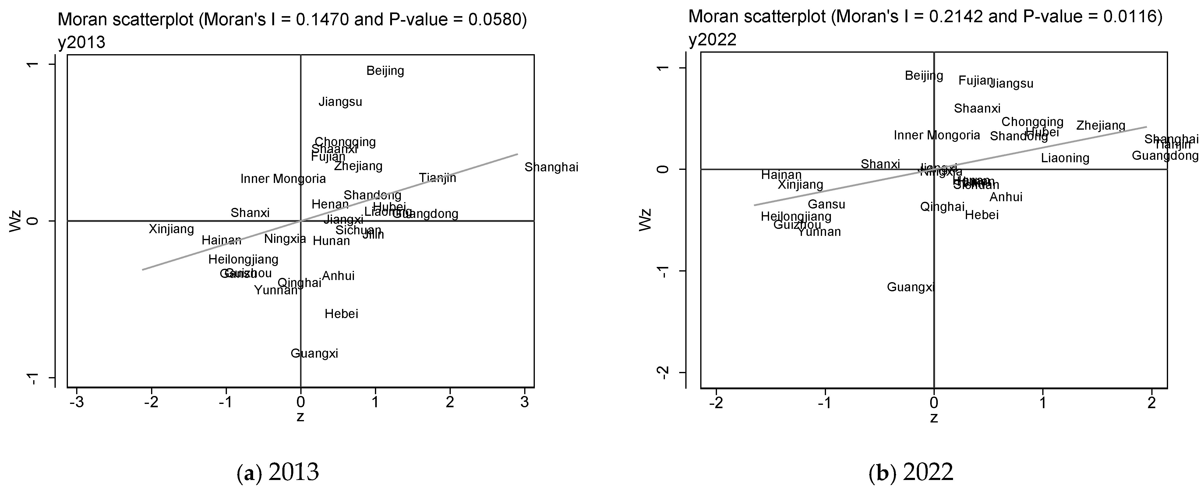
The Moran scatter plot divides China’s 30 provinces into four quadrants based on the industrial collaborative agglomeration characteristics of neighboring regions. The first quadrant, representing high–high agglomeration, indicates that both the local and neighboring regions have higher levels of industrial synergistic agglomeration. The second quadrant, showing low–high agglomeration, represents regions with a lower local level of industrial synergistic agglomeration, while neighboring areas exhibit a higher degree. The third quadrant, corresponding to low–low agglomeration, indicates that both the local and neighboring regions have lower levels of industrial collaborative agglomeration. The fourth quadrant, representing high–low agglomeration, shows regions with significant local industrial synergistic agglomeration but low neighboring industrial collaborative agglomeration. As shown in Figure 1, in 2013 and 2022, the majority of China’s provinces fall within the first and third quadrants, exhibiting high–high and low–low agglomeration, which reflects a positive spatial correlation in industrial collaborative agglomeration. Compared to 2013, by 2022, the positions of the provinces are farther from the origin, indicating a stronger spatial effect.

4.2. Analysis of the Static Spatial Panel Model

The analysis of geographical autocorrelation reveals a positive spatial correlation in industrial collaborative agglomeration, suggesting that the construction of the spatial econometric model is appropriate. The LM test and Hausman test were conducted to determine the suitable static spatial econometric model, with results presented in

Table 4. Results of model setting test.

Test	Statistic
LM-lag	9.320 ***
Robust LM-lag	10.344 ***
LM-error	1.992
Robust LM-error	3.016 *

Note: *** and * indicate significance at the 1 and 10% levels.

. The LM-lag is significant, while the LM-error is not, indicating that the SAR is the more appropriate choice. The results of the Hausman test suggest that a fixed-effects model is most suitable.

Following the methodology of Lee et al. [62], the model constructed in this paper is estimated, with the regression results presented in column (1) of

Table 5. Estimation results of the static spatial panel model.

Variable	(1)	(2)	(3)	(4)
	Main	LR_ Direct	LR_ Indirect	LR_ Total
Dig	−0.0999 ***	−0.1012 ***	−0.0457 **	−0.1469 ***
	(−4.23)	(−4.12)	(−2.14)	(−3.82)
Tec	0.0072	0.0071	0.0033	0.0104
	(1.24)	(1.23)	(1.00)	(1.18)
Env	0.0436 **	0.0464 ***	0.0211 *	0.0675 **
	(2.41)	(2.61)	(1.74)	(2.48)
FDI	−0.0004	−0.0005	−0.0003	−0.0008
	(−0.07)	(−0.10)	(−0.11)	(−0.11)
Cit	0.1784 **	0.1813 **	0.0832	0.2645 **
	(2.00)	(2.10)	(1.45)	(1.99)
Res	0.0114 *	0.0120 **	0.0055	0.0176 *
	(1.93)	(1.97)	(1.42)	(1.88)
rho	0.3177 ***
	(3.61)
sigma2_e	0.0027 ***
	(12.14)
$R^2$	0.1136

Note: ***, **, and * indicate significance at the 1, 5, and 10% levels, with z-values in brackets.

. The parameter estimates from the SAR model do not directly reflect the direct effect and spatial spillover effect of the digital economy on industrial collaborative agglomeration. Therefore, partial differential decomposition is applied to partition the coefficients into direct, indirect, and total effects. The decomposition results for the spatial effects of each variable on industrial cooperative clustering are shown in columns (2)–(4) of Table 5.

Column (1) of Table 5 shows that the digital economy has a significant inhibiting effect on industrial collaborative agglomeration. This suggests that as the digital economy expands, geographic constraints weaken, allowing firms to collaborate and transact via the Internet rather than being tied to specific geographic locations, thus reducing the need for geographic agglomeration.

The direct effect reflects the impact of the digital economy on local industrial collaborative agglomeration, while the indirect effect indicates its influence on neighboring areas. The regression coefficient for the direct effect of the digital economy is −0.1012, significant at the 1% level, meaning a 1-unit increase in the digital economy leads to a 0.1012-unit decline in local industrial collaborative agglomeration. The coefficient for the indirect effect is −0.0457, significant at the 5% level, implying that a 1-unit rise in the digital economy results in a 0.0457-unit decrease in industrial collaborative agglomeration in neighboring regions. Moreover, due to feedback effects, the impact on neighboring regions further reduces local industrial collaborative agglomeration by 0.0013 units. Thus, the digital economy affects industrial collaborative agglomeration through geographic spillover effects, with intra-regional spillover effects being more pronounced than inter-regional ones.

The coefficients for the direct and total effects of environmental regulation, urbanization level, and innovation resource allocation are all significantly positive, indicating that stronger environmental regulations, higher levels of urbanization, and better allocation of innovation resources all contribute to improved industrial collaborative agglomeration.

4.3. Analysis of the Dynamic Spatial Panel Model

Table 6. Dynamic spatial lag model estimation results.

Variable	(1)	(2)	(3)	(4)	(5)	(6)	(7)
	Main	SR_ Direct	SR_ Indirect	SR_ Total	LR_ Direct	LR_ Indirect	LR_ Total
L. y	0.8992 ***
	(21.4253)
L. Wy	1.2101 ***
	(9.5910)
Dig	−0.0748 **	−0.0721 **	−0.0246	−0.0966 *	−0.0925 *	0.1450 **	0.0525 **
	(−2.0657)	(−2.0463)	(−1.2706)	(−1.9107)	(−1.8069)	(1.9635)	(2.0469)
Dig2	−0.0231 ***	−0.0227 ***	−0.0077	−0.0304 **	−0.0291 **	0.0456 ***	0.0165 ***
	(−2.8576)	(−2.7623)	(−1.4538)	(−2.4929)	(−2.2893)	(2.5920)	(2.7488)
Tec	0.0146 ***	0.0147 ***	0.0048*	0.0195 ***	0.0186 ***	−0.0294 ***	−0.0108 ***
	(3.4532)	(3.5934)	(1.7297)	(3.3403)	(2.9466)	(−3.4226)	(−3.3760)
Env	−0.0001	0.0002	0.0002	0.0004	0.0005	−0.0006	−0.0001
	(−0.0064)	(0.0186)	(0.0412)	(0.0255)	(0.0266)	(−0.0223)	(−0.0140)
FDI	−0.0070 *	−0.0072 *	−0.0023	−0.0095 *	−0.0091 *	0.0143 *	0.0053 *
	(−1.8119)	(−1.7678)	(−1.2695)	(−1.7339)	(−1.6449)	(1.7378)	(1.7330)
Cit	0.2122 ***	0.2123 ***	0.0704	0.2827 ***	0.2698 ***	−0.4251 ***	−0.1553 ***
	(3.1694)	(3.2450)	(1.6027)	(2.9788)	(2.6910)	(−3.0986)	(−3.0984)
Res	0.0034	0.0038	0.0012	0.0050	0.0048	−0.0075	−0.0028
	(0.8358)	(0.9500)	(0.7492)	(0.9269)	(0.9039)	(−0.9352)	(−0.9487)
rho	0.2432 **
	(2.4690)
sigma2_e	0.0013 ***
	(12.8874)
$R^2$	0.7902	0.7902	0.7902	0.7902	0.7902	0.7902	0.7902

Note: ***, **, and * indicate significance at the 1, 5, and 10% levels, with z-values in brackets.

presents the regression results for the dynamic spatial lag model. Compared to the static model with an R² value of 0.1136, the dynamic model exhibits a significantly higher R² of 0.7902, indicating a better fit. In the dynamic spatial lag model, the coefficient of the squared term for the digital economy is −0.0231, significant at the 1% level. This suggests that the relationship between the digital economy and industrial collaborative agglomeration follows an inverted “U” shape, initially promoting and then inhibiting agglomeration.

The coefficient for the time lag term of industrial collaborative agglomeration is 0.8992, significant at the 1% level, indicating that past industrial collaborative agglomeration plays a crucial role in fostering current agglomeration. The coefficient for the spatio-temporal lag term of industrial collaborative agglomeration is 1.2101, also significant at the 1% level, suggesting that industrial collaborative agglomeration in neighboring regions positively influences agglomeration within a given region. This points to a positive spatial spillover effect among provinces, consistent with the high–high and low–low agglomeration patterns identified in the Moran scatterplot.

The spatial lag model coefficients do not directly capture the effects of explanatory variables on both the region and its neighboring regions, so partial differential decomposition is necessary to evaluate the direct, indirect, and total effects [63]. Columns (2)–(4) in Table 6 show the short-term direct, indirect, and total effects, while columns (5)–(7) present the long-term effects. The regression coefficients for the long-term effects are more significant than for the short-term effects, which is expected, as industrial synergistic agglomeration involves a time lag.

From a short-term perspective, the effect of the digital economy on industrial collaborative agglomeration is initially positive and then negative, indicating an inverted U-shaped nonlinear relationship. The short-term direct, indirect, and total effects of technological innovation on industrial collaborative agglomeration are all significantly positive, with the direct effect being greater than the indirect effect. This suggests that technological innovation fosters industrial collaborative agglomeration both locally and in neighboring regions. The coefficient for the short-term impact of environmental regulation is positive but not statistically significant. Foreign direct investment shows negative short-term direct, indirect, and total effects on industrial collaborative agglomeration, with the direct effect being more significant. This indicates that foreign direct investment inhibits local industrial agglomeration and has little impact on neighboring regions.

The short-term direct, indirect, and total effects of urbanization on industrial collaborative agglomeration are all positive, with the direct and total effects being significant, while the indirect effect is not. This suggests that increased urbanization boosts local industrial agglomeration, with minimal impact on neighboring areas. The coefficients for the short-term effects of innovation resource allocation are positive but insignificant, indicating that while higher innovation resource allocation may enhance industrial agglomeration to some extent, it does not have a substantial impact.

From a long-term perspective, the coefficient for the long-term direct effect of the squared term for the digital economy is −0.0291, significant at the 5% level, indicating an inverted U-shaped effect on local industrial collaborative agglomeration. The long-term indirect effect coefficient is 0.0456, significant at the 1% level, showing that the spillover effect of the digital economy on neighboring regions’ industrial agglomeration follows a U-shaped pattern. As the digital economy grows, the spillover effect shifts from a “siphon effect” to a “radiation effect”, with the long-term indirect effect surpassing the direct effect. Thus, the total long-term effect demonstrates a U-shaped nonlinear relationship.

4.4. Endogenous Problems

The explanatory variable and the explained variable may exhibit a causal relationship, potentially complicated by omitted variable bias, leading to endogeneity issues. To address this, the instrumental variable (IV) method is employed. Drawing on the research of Huang et al. [64], this study selects the 1984 historical data on the number of post offices as an instrumental variable. Prior to the widespread adoption of the Internet and the proliferation of fixed telephones, information transmission predominantly relied on postal services. Additionally, early information and communication technologies, such as fixed telephones, were managed by post offices, and the distribution of post offices influenced subsequent Internet access and digital infrastructure development. Consequently, the 1984 post office count satisfies the relevance criterion as an instrumental variable. Moreover, the 1984 post office count does not directly affect the collaborative agglomeration of manufacturing and producer services, fulfilling the exogeneity condition.

Given that this study analyzes panel data and the 1984 post office count is a time-invariant variable, we adopt the approach proposed by Nunn and Qian [65] to reflect the time-varying characteristics of the instrumental variable. Specifically, we incorporate the total volume of telecom services in each province during the study period. The total telecom service volume does not exert a direct influence on enterprise collaborative agglomeration, thus meeting the exogeneity requirement. Furthermore, it partially reflects the development level of the digital economy, satisfying the relevance condition. In summary, the multiplicative term (post × T), combining the 1984 post office count and the provincial total telecom service volume, is selected as the instrumental variable for the digital economy.

Table 7. Endogeneity test results.

	(1)	(2)	(3)	(4)	(5)	(6)
	No Control Variables			Control Variables Added
	2SLS First-Stage Regression		2SLS Second-Stage Regression	2SLS First-Stage Regression		2SLS Second-Stage Regression
	Dig	Dig2		Dig	Dig2
Dig			−0.3078 *			−0.2854 *
			(−1.29)			(−1.57)
Dig2			−0.1437 **			−0.0904 *
			(−2.44)			(−1.84)
post × T	−0.9149 ***	1.8282 **		−0.9694 ***	2.0345 ***
	(−4.77)	(2.39)		(−6.45)	(3.25)
$({\mathrm{p}\mathrm{o}\mathrm{s}\mathrm{t}\times \mathrm{T})}^2$	0.0342 ***	−0.0856 ***		0.0317 ***	−0.0758 ***
	(6.24)	(−3.91)		(7.40)	(−4.26)
Unrecognizable inspection
Kleibergen–Paap rk LM statistic	20.118 ***			17.311 ***
Weak instrumental variable test
Minimum eigenvalue statistic	34.8852			26.5585
Kleibergen–Paap rk Wald F statistic	28.657 ***			21.774 ***
Cragg–Donald Wald F statistic	68.265 ***			26.310 ***
	[7.03]			[7.03]
Robust weak identification test
Anderson–Dubin Wald test	23.2033 ***			20.4563 ***
Wu–Hausman F	12.3646 ***			10.6107 ***
statistic	300	300	300	300	300	300
$R^2$	0.5971	0.6041	0.1667	0.7655	0.7498	0.5447

Note: ***, **, and * are significant at the level of 1, 5, and 10%, with t-values in brackets. The value in square brackets is the critical value of the Stock–Yogo weak instrumental variable test at the level of 10%.

presents the results of the endogeneity test. Columns (1)–(3) display the regression outcomes of the IV test without control variables, while columns (4)–(6) present the results after incorporating control variables. The Kleibergen–Paap rk LM statistic is significant at the 1% level, indicating a robust correlation between the instrumental variables and the endogenous explanatory variables. The minimum eigenvalue statistic from the weak IV test exceeds 10, passing the rule-of-thumb threshold for weak instruments. Both the Kleibergen–Paap rk Wald F statistic and the Cragg–Donald Wald F statistic surpass the 10% maximum IV size, confirming that the instrumental variables are not weak. With the number of instrumental variables equal to the number of endogenous explanatory variables and a Hansen J statistic value of 0.000, there is no evidence of over-identification. The Anderson–Rubin Wald test statistic rejects the null hypothesis at the 1% level, asserting that the IV is sufficiently identified. Based on the regression results in columns (3) and (6), the quadratic term of the digital economy exhibits a significantly negative coefficient, aligning with prior estimation findings and validating the reliability of the conclusions drawn in this paper.

4.5. Robustness Tests

(1)

Increasing control variables: Industrial collaborative agglomeration is affected by transportation costs. Therefore, transportation cost (Trac) is added as a control variable and measured by the reciprocal of road density [66]. The regression results are shown in Table 8 (1).

(2)

Replacement of the spatial weight matrix: A dynamic spatial econometric regression is conducted using the economic–geographic nested matrix $W_2$ as the spatial weight matrix. The results of this analysis are shown in Table 8 (2).

The economic geography nesting matrix $W_2$ is calculated as follows:

$$W_{2ij}=\left\{\begin{array}{ll}0.5\times W_{ij}^d+0.5\times W_{ij}^e& i\ne j\\ 0& i=j\end{array}\right.$$

(32)

where $W_{ij}^d$ denotes the inverse geographic distance matrix and $W_{ij}^e$ represents the economic distance matrix.

(3)

Excluding the abnormal year: In 2020, China experienced an outbreak of the COVID-19 epidemic. The epidemic situation across the country was severe in 2022, which severely impacted the national economy and industries. There was a time lag effect in the industrial collaborative agglomeration. As a result, the data from 2022 may be considered an outlier and could potentially affect the research conclusions. After excluding the 2022 data, the dynamic spatial lag model regression is re-estimated, with the results presented in Table 8 (3). The regression coefficient for the square term of the digital economy remains consistent with previous findings, indicating that the result is robust.

(4)

Replacing the calculation method of the explained variable: To further verify the robustness of the parameters of the improved industrial collaborative agglomeration index, the traditional calculation approach for the industrial collaborative agglomeration index (as shown in Equation (2)) was employed for recalculations, followed by dynamic spatial lag model regression analysis. The regression results are presented in Table 8 (4). The sign of the regression coefficient of the square term of the digital economy is consistent with the previous conclusion, indicating that the parameters are robust.

Table 8. Robustness test.

	Variable	Main	SR_ Direct	SR_ Indirect	SR_ Total	LR_ Direct	LR_ Indirect	LR_ Total
(1)	L. y	0.9673 ***
		(22.61)
	L. Wy	1.8631 ***
		(15.22)
	Dig	0.5120 ***	0.5709 ***	0.6611 *	1.2320 **	0.8261 ***	−1.0498 ***	−0.2237 ***
		2.78)	(2.99)	(1.70)	(2.30)	(3.02)	(−3.03)	(−3.03)
	Dig2	−0.5902 ***	−0.6551 ***	−0.7613 *	−1.4164 **	−0.9477 ***	1.2043 ***	0.2566 ***
		(−3.15)	(−3.43)	(−1.73)	(−2.43)	(−3.49)	(3.50)	(3.50)
	Trac	0.0005	0.0007	0.0008	0.0014	0.0009	−0.0012	−0.0003
		(0.27)	(0.34)	(0.30)	(0.32)	(0.34)	(−0.34)	(−0.34)
	rho	0.5444 ***
		(5.54)
	sigma2_e	0.0013 ***
		(12.85)
	$R^2$	0.6695
(2)	L. y	0.8968 ***
		(20.9731)
	L. Wy	2.1256 ***
		(16.0580)
	Dig	−0.0248	−0.0228	−0.0282	−0.0510	−0.0150	0.0232	0.0082
		(−0.6908)	(−0.6192)	(−0.5547)	(−0.5999)	(−0.4788)	(0.5573)	(0.6140)
	Dig2	−0.0238 ***	−0.0247 ***	−0.0289	−0.0537 **	−0.0148	0.0239	0.0090 ***
		(−3.0068)	(−2.8851)	(−1.5455)	(−2.1277)	(−1.0181)	(1.5187)	(2.9154)
	rho	0.5360 ***
		(5.1049)
	sigma2_e	0.0013 ***
		(12.8396)
	$R^2$	0.6459
(3)	L. y	0.9539 ***
		(21.46)
	L. Wy	1.8456 ***
		(13.68)
	Dig	1.5176 ***	1.8944 **	6.4929	8.3873	2.6601 ***	−3.2679 ***	−0.6079 ***
		(4.67)	(2.15)	(0.29)	(−0.37)	(3.22)	(−3.69)	(−4.85)
	Dig2	−1.2565 ***	−1.5800 *	−5.4783	−7.0583	−2.2159 ***	2.7220 ***	0.5061 ***
		(−3.64)	(−1.93)	(−0.28)	(−0.34)	(−2.87)	(3.20)	(3.94)
	rho	0.7506 **
		(6.52)
	sigma2_e	0.0031 ***
		(12.18)
	$R^2$	0.7157
(4)	L.y	0.9354 ***
		(19.22)
	L.Wy	1.1946 ***
		(6.78)
	Dig	0.3992 ***	0.4212 ***	0.2480	0.6692 ***	0.8369 ***	−1.1152 ***	−0.2782 ***
		(2.90)	(3.14)	(1.55)	(2.61)	(2.72)	(−2.96)	(−3.01)
	Dig2	−0.3066 **	−0.3267 ***	−0.1931	−0.5198 **	−0.6495 **	0.8652 **	0.2156 **
		(−2.25)	(−2.51)	(−1.41)	(−2.17)	(−2.24)	(2.40)	(2.45)
	rho	0.3558 ***
		(2.98)
	sigma2_e	0.0006 ***
		(12.79)
	$R^2$	0.4122

Note: ***, **, and * indicate significance at the 1, 5, and 10% levels, with z-values in brackets.

Table 8. Robustness test.

	Variable	Main	SR_ Direct	SR_ Indirect	SR_ Total	LR_ Direct	LR_ Indirect	LR_ Total
(1)	L. y	0.9673 ***
		(22.61)
	L. Wy	1.8631 ***
		(15.22)
	Dig	0.5120 ***	0.5709 ***	0.6611 *	1.2320 **	0.8261 ***	−1.0498 ***	−0.2237 ***
		2.78)	(2.99)	(1.70)	(2.30)	(3.02)	(−3.03)	(−3.03)
	Dig2	−0.5902 ***	−0.6551 ***	−0.7613 *	−1.4164 **	−0.9477 ***	1.2043 ***	0.2566 ***
		(−3.15)	(−3.43)	(−1.73)	(−2.43)	(−3.49)	(3.50)	(3.50)
	Trac	0.0005	0.0007	0.0008	0.0014	0.0009	−0.0012	−0.0003
		(0.27)	(0.34)	(0.30)	(0.32)	(0.34)	(−0.34)	(−0.34)
	rho	0.5444 ***
		(5.54)
	sigma2_e	0.0013 ***
		(12.85)
	$R^2$	0.6695
(2)	L. y	0.8968 ***
		(20.9731)
	L. Wy	2.1256 ***
		(16.0580)
	Dig	−0.0248	−0.0228	−0.0282	−0.0510	−0.0150	0.0232	0.0082
		(−0.6908)	(−0.6192)	(−0.5547)	(−0.5999)	(−0.4788)	(0.5573)	(0.6140)
	Dig2	−0.0238 ***	−0.0247 ***	−0.0289	−0.0537 **	−0.0148	0.0239	0.0090 ***
		(−3.0068)	(−2.8851)	(−1.5455)	(−2.1277)	(−1.0181)	(1.5187)	(2.9154)
	rho	0.5360 ***
		(5.1049)
	sigma2_e	0.0013 ***
		(12.8396)
	$R^2$	0.6459
(3)	L. y	0.9539 ***
		(21.46)
	L. Wy	1.8456 ***
		(13.68)
	Dig	1.5176 ***	1.8944 **	6.4929	8.3873	2.6601 ***	−3.2679 ***	−0.6079 ***
		(4.67)	(2.15)	(0.29)	(−0.37)	(3.22)	(−3.69)	(−4.85)
	Dig2	−1.2565 ***	−1.5800 *	−5.4783	−7.0583	−2.2159 ***	2.7220 ***	0.5061 ***
		(−3.64)	(−1.93)	(−0.28)	(−0.34)	(−2.87)	(3.20)	(3.94)
	rho	0.7506 **
		(6.52)
	sigma2_e	0.0031 ***
		(12.18)
	$R^2$	0.7157
(4)	L.y	0.9354 ***
		(19.22)
	L.Wy	1.1946 ***
		(6.78)
	Dig	0.3992 ***	0.4212 ***	0.2480	0.6692 ***	0.8369 ***	−1.1152 ***	−0.2782 ***
		(2.90)	(3.14)	(1.55)	(2.61)	(2.72)	(−2.96)	(−3.01)
	Dig2	−0.3066 **	−0.3267 ***	−0.1931	−0.5198 **	−0.6495 **	0.8652 **	0.2156 **
		(−2.25)	(−2.51)	(−1.41)	(−2.17)	(−2.24)	(2.40)	(2.45)
	rho	0.3558 ***
		(2.98)
	sigma2_e	0.0006 ***
		(12.79)
	$R^2$	0.4122

Note: ***, **, and * indicate significance at the 1, 5, and 10% levels, with z-values in brackets.

4.6. Heterogeneity Analysis

The regional economic foundations differ significantly across China. In the eastern region, the digital economy developed earlier, with widespread industrial clusters, while some provinces in the central region have taken the lead in advancing the digital economy and establishing digital computing bases and big data centers. In contrast, the western region faces weaker digital infrastructure and a relatively underdeveloped industrial sector. As a result, the impact of the digital economy on industrial collaborative agglomeration varies across regions.

Table 9. Analysis of regional heterogeneity.

Variable	West	Central						East
	OLS	SAR-SR_ Direct	SAR-SR_ Indirect	SAR-SR_ Total	SAR-LR_ Direct	SAR-LR_ Indirect	SAR-LR_ Total	SAR-LR_ Direct	SAR-LR_ Indirect	SAR-LR_ Total
Dig	0.5971 ***	0.2040 ***	−0.0710 ***	0.1330 ***	−0.0449 ***	−0.0076 ***	−0.0525 ***	−0.1163 **	0.0341 *	−0.0823 **
${Dig}^2$	0.1433 ***
Tec	−0.0011	−0.0115 ***	0.0041**	−0.0074 ***	0.0025 ***	0.0004 **	0.0029 ***	0.0130	−0.0036	0.0094
Env	0.2801 ***	−0.1020 ***	0.0358 ***	−0.0661 ***	0.0224 ***	0.0038 ***	0.0262 ***	−0.0910 **	0. 0254	−0.0656 **
FDI	0.0161 *	−0.0314 ***	0.0111 ***	−0.0204 ***	0.0069 ***	0.0012 ***	0.0081 ***	0.0049	−0.0012	0.0037
Cit	0.4188 ***	−0.2583 ***	0.0912 **	−0.1671 ***	0.0568 ***	0.0097**	0.0665 ***	0.5614 ***	−0.1616	0.3998 ***
Res	0.0132	0.0221 ***	−0.0077 ***	0.0144 ***	−0.0049 ***	−0.0008 ***	−0.0057 ***	0.0256 **	−0.0073	0.0183 **
$R^2$	0.7108	0.9284						0.2015
rho		−0.4921 ***						−0.3707 **

Note: ***, **, and * indicate significance at the 1, 5, and 10% levels.

presents the results of the digital economy’s influence on industrial collaborative agglomeration in the western, central, and eastern regions of China. In the western region, the digital economy is underdeveloped, and industrial collaborative agglomeration is slow to grow. The spatial spillover effects are minimal, making the OLS model more suitable for estimation. For the central region, the SAR model is selected, but the model fit worsens when the square term of the digital economy is added, indicating no nonlinear correlation between the digital economy and industrial collaborative agglomeration. In the eastern region, the static spatial lag model is used, but the model fit deteriorates when the square term of the digital economy is included, suggesting the absence of a nonlinear relationship in this area. Table 9 presents the estimation results for the impact of the digital economy on industrial collaborative agglomeration in these three regions.

In the western region, the coefficient of the square term for the digital economy is 0.1433, significant at the 1% level, indicating a U-shaped nonlinear relationship between the digital economy and industrial collaborative agglomeration. In the central region, the rho value is significantly negative, suggesting a strong negative spillover effect of industrial collaborative agglomeration, with the “siphon effect” being particularly noticeable. In the short term, the digital economy fosters industrial collaborative agglomeration within the region but inhibits it in neighboring areas, highlighting the pronounced “siphon effect.” In the long term, the digital economy significantly hampers industrial collaborative agglomeration in both local and adjacent areas. In the eastern region, the direct effect coefficient of the digital economy is significantly negative, indicating that its growth will hinder industrial collaborative agglomeration. However, the indirect effect coefficient is significantly positive, showing that the digital economy will stimulate industrial collaborative agglomeration in neighboring regions, thereby demonstrating a clear “radiation effect” from the eastern region and encouraging industrial dispersion to neighboring areas.

5. Discussion

This paper examines the impact of the digital economy on industrial collaborative agglomeration using panel data from 30 Chinese provinces between 2013 and 2022. The analysis includes the development of a digital economy measurement index system and an evaluation of collaborative agglomeration indices. The main conclusions are as follows:

Firstly, from a short-term perspective, the effect of the digital economy on industrial collaborative agglomeration follows an inverted “U” shape, which is consistent with the findings of Ma et al. regarding the influence of the digital economy on industrial agglomeration [67]. The digital economy fosters the growth of the information technology service industry, drives technological innovation, and attracts talent, which in turn brings productive service firms into the fold. This reduces production, transaction, and service costs, while providing access to more advanced technology and knowledge. Consequently, manufacturing enterprises join the agglomeration, boosting industrial collaboration. However, as industrial agglomeration intensifies, the number of enterprises grows and the region’s carrying capacity becomes constrained, leading to heightened environmental pressures. Additionally, the digital economy allows enterprises to exchange information online in a cost-effective manner, reducing the need to remain in the agglomeration area and enabling firms to establish operations in other locations, thereby decreasing industrial collaborative agglomeration levels. These findings contrast with those of Huang et al., who concluded that the digital economy positively impacts industrial agglomeration [32,33], and Xu and Zhao, who found that the digital economy improves industrial collaboration through technological innovation and resource efficiency [32]. This discrepancy arises due to differences in research focus and periods.

Secondly, from a long-term perspective, the effect of the digital economy on local industrial collaborative agglomeration remains inverted “U”-shaped, but its impact on adjacent regions follows a “U” shape. Both the “siphon effect” and the “radiation effect” of the digital economy are present. The “siphon effect” refers to the dispersive force of industrial collaborative agglomeration in neighboring areas, while the “radiation effect” reflects its centripetal force. As the digital economy matures, the agglomeration force eventually surpasses the dispersive force, meaning that the long-term effect on industrial collaboration in surrounding areas initially inhibits growth before promoting it. The pioneering regions of the digital economy accumulate technological and resource advantages, attracting labor, capital, and technology from less developed neighboring regions, resulting in a negative spillover effect. However, once the digital economy reaches a certain level in the leading regions, issues such as population density, strained educational resources, traffic congestion, and fierce market competition arise. Digital technology accelerates the dissemination of knowledge and innovation, which enhances the agglomeration force in surrounding areas, leading to a positive spillover effect. Taking the Haier Industrial Park in Qingdao as a case study, this paper examines the evolutionary process of how the digital economy influences the collaborative agglomeration of industries. Initially, the park was dominated by traditional manufacturing sectors such as refrigerators and air conditioners. Geographical proximity facilitated information and technology sharing, thereby reducing operational costs. Over time, various entities entered the park, including Haier University, research and development centers, financial management hubs, Ririshun Supply Chain, biopharmaceutical enterprises, and energy headquarters. With advancements in the digital economy, the dissemination of digital information technology has transcended geographical boundaries. Leveraging digital technologies and Internet platforms, industrial collaborative clusters have expanded from Qingdao to neighboring regions such as Zibo and Jinan, and further radiated to provinces like Anhui, Sichuan, and Jiangxi via the Haier COSMOPlat, demonstrating significant spillover effects.

Thirdly, industrial collaborative agglomeration exhibits both significant time lag effects and spatial spillovers. Previous industrial agglomeration influences current levels of collaboration, with regional enhancements boosting neighboring areas. These effects can be positive or negative. Positive spillovers include knowledge and technology transfers, market scale effects, and more frequent talent flow, facilitating joint R&D activities and disruptive technological innovations. Once the agglomeration reaches a certain threshold, scale effects emerge, and neighboring regions strengthen ties with the core area, benefiting from its growth. On the other hand, negative spillovers manifest as environmental pressures and the siphoning effect, which exacerbates regional imbalances. Environmental pollution spreads, impacting neighboring areas, and the siphon effect can worsen regional disparities. However, when effectively regulated through policy, the positive spillovers of industrial agglomeration can outweigh the negative effects, promoting coordinated regional growth.

Fourthly, regional heterogeneity analysis reveals that the digital economy’s impact on industrial collaborative agglomeration varies across regions. In the western region, the impact is initially inhibitory but eventually becomes promotive. The region’s digital economy is underdeveloped, requiring significant investment in infrastructure, which hinders the formation of industrial agglomeration. Once the digital economy reaches a certain threshold, scale effects and lower entry costs encourage business clustering, thus enhancing industrial collaboration. However, due to its geographical remoteness, the western region struggles with generating spatial spillovers. In the central region, the digital economy has a short-term positive impact but exerts long-term inhibitory effects, with a pronounced “siphoning effect” in neighboring regions. In the eastern region, the digital economy inhibits local industrial agglomeration but promotes it in adjacent regions, reflecting a more pronounced “radiation effect”. While the eastern region’s high level of industrial agglomeration leads to issues such as environmental pollution, traffic congestion, and rising costs, digital technology and knowledge spillovers facilitate the geographic dispersion of enterprises, encouraging industrial growth in surrounding areas.

Lastly, there are some limitations in this study. Firstly, as an emerging economic paradigm, the digital economy faces limitations in data accessibility and is constrained by the technologies and tools utilized for data collection, which may result in potential issues regarding data quality. Secondly, while this paper investigates the digital economy’s impact, it lacks a deeper exploration of the underlying mechanisms. Future research should focus on these mechanisms and the paths through which the digital economy influences industrial agglomeration. Finally, this study primarily focuses on manufacturing and productive service industries, and the applicability of the findings to other sectors warrants further exploration.

6. Recommendation

This study proposes several policy recommendations to optimize the layout of industrial collaborative agglomeration and promote sustainable industrial economic development:

Firstly, resource allocation should be optimized to foster economies of scale. By aligning regional resource endowments with industrial strengths, regions can identify key industries to promote and develop long-term plans for establishing industrial clusters with scale advantages. Strengthening the links between supply and demand within clusters, attracting upstream and downstream industries, and improving the supply chain will enhance industrial synergy, increase agglomeration, and drive regional economic growth.

Secondly, digital and transportation infrastructure should be improved. To enhance connectivity, particularly in central and western regions, the government should increase subsidies, improve communication networks, and foster cross-regional cooperation. Based on the computational power requirements of the eastern region, large-scale data centers and computing power networks will be strategically deployed in the central and western regions to achieve the “East Data West Computing” initiative. Building a unified national digital platform will facilitate knowledge exchange and technological innovation, overcoming geographic barriers and creating a more integrated market.

Thirdly, high-level talent should be cultivated, and scientific innovation should be supported. The government should incentivize the integration of industry, academia, and research by offering subsidies for talent acquisition, such as housing, employment, and business start-up support. Encouraging R&D and innovation through financial incentives, loan preferences, and strong intellectual property protection will foster innovative industrial clusters and strengthen technology-driven enterprises. In addition to technological advancements, promoting innovation in management, marketing models, and branding is essential for broader industrial development. Emphasis will be placed on fostering local talent in the western region, while the eastern region periodically dispatches technical experts to provide support in the western region.

Finally, green and sustainable development should be promoted. A “carrot and stick” approach can be adopted to drive eco-friendly transformation. On one hand, the upgrading of traditional industries and the adoption of green technologies to reduce carbon emissions should be encouraged. On the other hand, stricter regulations on high-pollution and high-energy-consuming enterprises should be enforced, ensuring that only those meeting environmental standards receive approval for operation.