Article

Regional Integration, Technological Innovation, and Digital Economy: Evolution and Evidence of the Decarbonization Driving Forces in the Yangtze River Delta

School of Management, Shanghai University, Shanghai 200444, China
*
Author to whom correspondence should be addressed.
Sustainability 2025, 17(12), 5463; https://doi.org/10.3390/su17125463
Submission received: 9 April 2025 / Revised: 2 June 2025 / Accepted: 10 June 2025 / Published: 13 June 2025

Abstract

:
Economic decarbonization has gained attention as a viable way to achieve carbon neutrality without sacrificing high-quality economic development. Regional integration (RI), technological innovation (TI), and the digital economy (DIE) are important decarbonization driving forces. To analyze how they impact carbon reduction and the evolutionary patterns observed in urban development, this study focuses on the urban agglomeration of the Yangtze River Delta (YRD) and uses the spatial Durbin model (SDM) to decompose the carbon reduction effects into spatial spillover effects and short-term and long-term effects. The research findings include the following: (1) The decarbonization driving forces have promoted economic decarbonization in the YRD and exhibit distinct evolutionary patterns. (2) The decarbonization effects exhibit spatiotemporal heterogeneity depending on the economic situation, period, and energy status of the cities. Over time, TI and DIE demonstrate better decarbonization effects. Economically developed cities are more likely to expand their carbon reduction advantages, while cities with dense energy supplies struggle to achieve their full carbon reduction potential due to traditional energy structures. (3) Industrial structure upgrading (UIS) is a critical pathway through which TI and DIE reduce carbon emissions. These findings enrich existing research on decarbonization drivers and offer valuable insights for governments to formulate further policies for economic decarbonization.

1. Introduction

Sea level rise, extreme weather events, the destruction of ecosystems, and the increasing scarcity of resources owing to global warming pose a great threat to both the survival and development of humankind [1,2]. Carbon emissions contribute to over 60% of the greenhouse effect and have become a top priority for controlling climate change [3,4]. As a major global emitter of carbon and pollutants, China has relied heavily on traditional fossil fuels for energy supply, driving rapid economic growth over the past three decades at the cost of surging carbon emissions [5,6]. China’s total carbon emissions crept to 12,730.64 million tons in 2020 from 6827.46 million tons in 2005 [7], contributing approximately 30% of global emissions [8], while non-fossil fuels represented only 15.9% of its energy mix [9]. Despite setting “dual carbon” goals (carbon peak by 2030 and carbon neutrality by 2060), China’s energy structure remains reliant on fossil fuels in the short term, making economic decarbonization a central proposition for achieving green development. Therefore, exploring effective decarbonization drivers from multiple perspectives has become crucial for researchers seeking sustainable development solutions.
The existing literature has extensively explored decarbonization drivers. Drivers such as industrial structure [10,11], population density [12,13,14], economic growth [15], openness to foreign trade [16,17], China’s market-oriented reforms [18,19], government policies [20], energy intensity, and energy mix [11] have been found to either promote or inhibit carbon emissions. Among them, RI, TI, and DIE have demonstrated remarkable carbon emission reduction potential under the promotion of the “dual carbon” goals and national policies. RI has been endowed with new connotations (regional economic and ecological integration) by national strategies such as the construction of a “Resource-conserving and Environment-friendly Society” and the “Beautiful China” initiative, enhancing resource efficiency through policy coordination [21,22]. As the core driver of the “Innovation-Driven Development” strategy, green TI promotes emission reduction by directly transforming green patents to upgrade industrial structures [23,24]. China’s “Digital China” strategy clearly states that “Digitization Drives Green Production Modes,” regarding DIE as a key vehicle to achieve the “dual carbon” goals, which amplifies the emission reduction achievements of technologies through a multiplier effect [25,26,27]. However, most studies focus on single drivers, and a consensus on their relationship with carbon emissions remains elusive. Moreover, due to China’s reform approach of implementing pilot programs before nationwide adoption, cities often exhibit diverse development characteristics. Consequently, the specific impacts of these three drivers on carbon emissions and their evolutionary patterns across different urban development stages remain underexplored. Addressing this knowledge gap holds significant implications for enriching socioeconomic decarbonization theories and informing scientifically grounded development planning.
This study focuses on the YRD urban agglomeration and employs spatial econometric models to systematically investigate the spatial dynamics and operational mechanisms of decarbonization drivers. The main contributions are as follows: (1) The respective carbon emission performance of RI, TI, and DIE was analyzed from the perspective of the spatial spillover effect. (2) The decarbonization effectiveness and evolution patterns of RI, TI, and DIE at the city level are examined in terms of the period, economic situation, and energy intensity heterogeneity. (3) The possible mechanisms of the decarbonization driving forces on carbon emissions by industrial structure upgrading are explored.
The remainder of the article is arranged as follows: Section 2 introduces the study area, variables, data, and methodologies. Section 3 reports the empirical results, including a heterogeneity analysis and mechanism analysis. Section 4 discusses the economic implications of the findings, their relationships with relevant research, and proposes policy recommendations alongside research limitations. Section 5 summarizes the key findings of this study. Figure 1 shows the main framework of the study.

2. Materials and Methods

2.1. Study Area

The YRD urban agglomeration, located in southeastern China, encompasses 26 cities across Shanghai Municipality and the provinces of Anhui, Jiangsu, and Zhejiang [28]. First, despite occupying less than 4% of China’s land area, the YRD generates nearly 25% of the nation’s GDP and one-third of its total import–export volume, making it the most economically robust, globally integrated, and strategically vital region in China [29]. The region’s population has grown steadily, comprising approximately one-eighth of China’s total population by 2021 [30]. However, like many economically developed and densely populated areas, the YRD faces profound conflicts between ecological protection and development imperatives [31]. Second, as a globally renowned manufacturing and trade hub, the YRD has a substantial share of labor-intensive and energy-intensive secondary industries [32]. Rapid urbanization and industrialization have driven a continuous rise in regional energy consumption, with fossil fuels dominating the energy structure [33]. Finally, the YRD has progressively shifted away from its traditional high-energy-consumption growth model in recent years. Concurrently, the Chinese government aims to establish the YRD as a demonstration zone for RI, emphasizing industrial synergy and innovation [34]. Further, the size of DIE in the YRD accounts for about 44% of the regional GDP [35]. Therefore, it is an ideal location to systematically study the decarbonization effectiveness of RI, TI, and DIE (as in Figure 2).

2.2. Variables

2.2.1. Dependent Variable

According to the research of [36,37,38,39], carbon emissions at the city level were calculated based on the IPCC (Intergovernmental Panel on Climate Change) carbon emission inventory and energy balance table. The carbon emissions (CE) of most cities showed a positive growth trend in the YRD (as in Figure 3). Then, the logarithmic value of carbon emissions was used as the dependent variable while eliminating heteroscedasticity.

2.2.2. Key Explanatory Variable

In this paper, it is necessary to find or construct proxy variables as key explanatory variables to indicate the development level of RI, TI, and DIE, respectively. Since patent authorization better reflects the actual improvement of technology [40], this paper selects green invention patent authorizations to reflect the technological innovation capacity to capture the dynamics of green innovation in society. The technological innovation capacity of the cities in the YRD cluster is growing overall, with a few “peak” cities experiencing rapid growth and other “slow” cities experiencing small increases (as in Figure 4). Figure 5 depicts the spatial and temporal changes in technological innovation in the cities of the YRD, as mapped by ArcGIS 10.8. It can be seen that over time, the spatial agglomeration effect of high-level regions has become more obvious, forming a technological innovation plateau centered on the “peak” cities (such as Shanghai, Hangzhou, and Nanjing), while the gap within the region has also widened.
The level of RI and the development of DIE are measured by a composite system of evaluation indicators. Table 1 displays the measurement indicator system of the regional integration, including two levels of social and economic life. This paper incorporates 17 indicators in the areas of public services, human capital, and ecological construction, making the evaluation of regional integration more reasonable. Public services are related to the quality of life and social welfare of residents, and this indicator can measure the level and balance of various public services provided by the government for residents in the region. Human capital is one of the core elements of regional economic development, and this indicator is selected to reflect the quality and ability of the labor force in the region. In order to measure the degree of attention paid to the ecological environment and the effectiveness of its protection in the process of economic development, the indicator on ecological construction is used to assess the state of ecological environmental protection and sustainable development in the region. The urban green coverage area reflects the government’s efforts to increase carbon sinks. The domestic waste disposal rate reflects the sanitary conditions of the city. In addition, the literature has pointed out that reducing pollution has similarities with carbon emissions in addressing climate change and sustainable economic development [41,42]. Given data availability, future research could supplement other pollutant emission or treatment indicators to reflect the efforts of local governments in ecological governance more accurately. This comprehensive indicator is calculated using the entropy weight (EW) method.
Figure 6 represents the spatiotemporal evolution of RI in the YRD city cluster in 2011, 2016, and 2021. During the study period, the level of RI in the urban agglomeration increases significantly and shows regional synergies. The high-value area gradually expands and focuses on the core cities. In terms of the spatial pattern, the high-value areas are mainly concentrated in Southern Jiangsu and Shanghai. The change reflects the increasing capacity for regional cooperation and harmonious development of the cities in the YRD driven by the integration strategy and also reveals that there are still some development gaps between the regions.
As shown in Table 2, DIE has spawned potential growth drivers in the logistics industry over the past decade. Therefore, adding the express delivery business indicator to the traditional internet and communication indicators can more scientifically reflect the scale of digital applications. A principal component analysis (PCA) is used for evaluation.
The overall level of DIE in the cities of the YRD cluster increased yearly over the study period, with regional differences gradually narrowing (as shown in Figure 7). In view of the spatial pattern, the high-value areas are mainly concentrated in the central cities of Hangzhou, Nanjing, and Shanghai and spread to the periphery of the surrounding cities, with these core cities as the center. Over time, areas such as Wuxi, Hefei, and Jinhua also witnessed significant DIE growth, leading to a leveling of development gradients across regions. This spatial diffusion and equalization signify a transition from single-core to multi-core DIE development within the YRD, propelling regional integration and coordinated growth.

2.2.3. Other Variables

Studying the drivers of decarbonization in such a systematic framework requires a consideration of other important factors in carbon emissions. The population density (PD), GDP per capita (PGDP), and actual utilized foreign investment (FAI) are selected to represent population, economic prosperity, and openness in the rapid urbanization of China [20,45,54]. The efficiency of resource allocation is frequently discussed with market-oriented reform in China [18,19]. However, it remains unclear how the marketization level (ML) impacts carbon emissions. Therefore, referring to existing studies, the share of private and individual employees in the urban workforce was adopted to measure the ML [19]. The general public financial budget expenditures (FE) and R&D investments (RD) are utilized to indicate the behavior of the government in maintaining social operations and promoting reforms [20]. In addition, while the structure of the energy supply may not undergo rapid transformation, energy supply efficiency (ESE) is an indispensable factor in the study of carbon emissions. ESE is evaluated using the ratio of GDP to the total social electricity, LPG, and total gas supply after conversion to standard coal [5]. Finally, industrial structural upgrading (UIS) is used as a transmission variable to explore how decarbonization drivers affect carbon emissions through industrial reshaping. UIS was measured as the labor productivity ratio between the tertiary and secondary industries, referring to Wu et al.’s study [55].

2.3. Data Sources and Processing

This paper draws upon relevant professional research databases, primarily the China Stock Market & Accounting Research Database [56], China Emission Accounts and Datasets [57], and Chinese Research Data Services [58]. Other statistical information comes from the Provinces Statistics Yearbook, the China City Statistical Yearbook, the Cities Statistical Yearbook, etc. The GDP data are converted into constant prices in 2011. Any missing data are provided using interpolation and other fitting methods. This study used Stata 18.0 statistical analysis software. Table 3 presents the descriptive statistics of each variable, and the correlation coefficients between variables are shown in Table 4. To stabilize the data and mitigate heteroscedasticity, all variables were subjected to logarithmic transformation in subsequent experiments.

2.4. Methodology

First, the following fixed effects model was developed to investigate the “city–year” effect of the drivers of decarbonization.
L n C E i t = α 0 + α 1 K i t + α 2 C i t + μ i + υ t + ε i t
In the above equation, the subscripts i and t refer to the city and year, respectively, so L n C E i t (i.e., the dependent variable in this paper) represents the natural logarithm of carbon emissions for city i in year t . K i t refers to the key explanatory variables (i.e., the decarbonization driving forces in this paper). Depending on the driver of decarbonization, K i t is represented in Equation (1) as the variable for regional integration, technological innovation, and the digital economy, respectively. C i t denotes all control variables in the study. μ i and υ t control for city and year fixed effects, respectively. ε i t is a random disturbance term.
Then, this paper focuses on spatial econometric models based on the spatial spillover perspective. The spatial Durbin model (SDM) has significant advantages over the spatial error model (SEM) and spatial autoregressive model (SAR) in understanding spatial correlations and spillover effects and addressing omitted variables [59]. As a result, the SDM is a pleasant starting point in the framework of spatial economic analysis. The spatial panel Durbin model that controlled the “city–year” effect is as follows.
L n C E i t = β 0 + ρ W L n C E i t + β 1 K i t + λ 1 W K i t + β 2 C i t + λ 2 W C i t + μ i + υ t + ε i t
It is necessary to consider the specific impact of the spatial lag terms of the variables on the explanatory variables [60]. In order to avoid endogeneity issues and demonstrate the dynamic characteristics in carbon emission research, the dynamic SDM is developed to further improve the explanatory power.
L n C E i t = β 0 + ρ W L n C E i t + η W L n C E i t 1 + β 1 K i t + λ 1 W K i t + β 2 C i t + λ 2 W C i t + μ i + υ t + ε i t
In Equations (2) and (3), ρ is the spatial autoregressive coefficient, W is the spatial weight matrix, and W L n C E i t , W K i t , and W C i t represent the spatial lag terms of the corresponding variables. W L n C E i t 1 refers to the spatiotemporal associative lag term of carbon emissions. Other parameters are set as in Equation (1).
Finally, in order to understand the role played by UIS on carbon emissions, Equations (4)–(6) are combined, together with Equation (2), to explore possible transmission mechanisms [61].
L n U I S i t = γ 0 + ρ W U I S i t + γ 1 K i t + δ 1 W K i t + γ 2 C i t + δ 2 W C i t + μ i + υ t + ε i t
L n C E i t = γ 0 + ρ W L n C E i t + γ 3 U I S i t + δ 3 W U I S i t + γ 2 C i t + δ 2 W C i t + μ i + υ t + ε i t
L n C E i t = γ 0 + ρ W L n C E i t + γ 3 U I S i t + δ 3 W U I S i t + γ 1 K i t + δ 1 W K i t + γ 2 C i t + δ 2 W C i t + μ i + υ t + ε i t
Equations (4) and (5) test whether the key explanatory variables can significantly affect UIS and whether UIS significantly influences carbon emissions. Next, Equation (2) is combined with Equation (6) to test whether UIS is a transmission channel.
In addition, considering that the adjacency matrix does not easily express the spatial relationships of cities that are geographically close but not adjacent (e.g., Jiaxing and Shaoxing), the baseline regression to analyze spatial effects is based on the geographical distance matrix ( W 1 ). In the robustness test, the asymmetric economic geographic distance matrix ( W 2 ) is included to strengthen the role of city economic ties in the spatial effects.
W 1 = 1 / d i j , i j 0 , i = j
W 2 = W 1 × d i a g P 1 P ¯ , P 2 P ¯ , , P i P ¯
where d i j is the distance between the city i and j calculated based on latitude and longitude. P ¯ and P i denote the per capita GDP of the YRD and each city, respectively.

3. Results

3.1. Spatial Correlation Test

The spatial correlation test acts as a preliminary spatial data exploration. Before establishing a spatial econometric model, this study constructs a standardized geographic distance matrix ( W 1 ). Conducting Moran’s I index test and reporting the significance level in Table 5 can effectively show whether spatial autocorrelation exists. The Moran index value indicates that the carbon emissions in the YRD were significantly and spatially positively correlated from 2011 to 2021. Therefore, there was positive urban spatial dependency in carbon emissions in the last decade. Moran’s scatter plots in Figure 8 reflect the spatial heterogeneity of carbon emissions, indicating that spatial spillover is influenced by some social and economic drivers.

3.2. Benchmark Regression Results

The regression results of the ordinary least squares (OLS) method might not reflect the true relationship between the variables because of the spatial dependence of regional carbon emissions. In practical terms, carbon emissions from different geographic locations are related not only to the local area but also to other cities in space. To incorporate the city differences and period factors into account in the model, according to Equation (1), this study first uses the non-spatial fixed effects model (FE) in Table 6 to estimate the decarbonization driving forces.
Model 1 accounted for the city–year fixed effects. As Table 6 shows, the regression results of RI, TI, and DIE passed the Hausman test with a significance level of at least 5%, suggesting that the FE model was more appropriate than the random effects model (RE). The problem of heteroscedasticity among variables has also been avoided. The direct effect coefficient of RI is significantly negative at the 5% level, implying that a 1% increase in RI leads to a decrease of 0.1140 logarithmic percentage points in carbon emissions. Conversely, the direct effect coefficients of TI and DIE are significantly positive at the 1% level, implying that a 1% increase in their respective levels results in respective increases of 0.1329 and 0.1282 logarithmic percentage points in carbon emissions. Among the control variables, both PD and PGDP show significantly positive coefficients, suggesting their stimulating effects on carbon emissions. This demonstrates that urbanization and economic growth serve as drivers of carbon emissions. The significantly positive coefficient of ESE further exacerbates carbon emissions, reflecting that reliance on fossil energy remains challenging to reverse in the short term. However, the FE model renders it difficult to explain the spatial correction between explanatory variables and the dependent variable of neighboring units, so the estimation results are also biased. For example, some local governments have strongly emphasized economic development, and fiscal expenditures have increased year after year. The development climax of the traditional infrastructure triggered by fixed assets investment has resulted in huge amounts of carbon emissions. Because of the competition among local governments, the adverse effects of carbon emissions may be boosted. Therefore, while controlling for city-level differences, there is an urgent need for spatial econometric modeling to explore similar spatial relationships to those mentioned above.
The SDM provides a comprehensive understanding of the spatial spillover effect on carbon emissions and has a more accurate statistical performance. It reported more complex spatial linkages in the decarbonization driving forces of the YRD, and the static estimation results are given in Table 7. In general, the carbon emissions indicated negative spatial spillover effects due to significantly negative spatial autoregressive coefficients. This is consistent with the “low–high” value aggregation characteristic of carbon emissions reflected in the Moran scatter plot, further supporting the need to establish spatial joint prevention and control emission reduction strategies to avoid “carbon leakage” in some cities.
The Chi values of the Hausman test, LR test, and Wald test shown in Table 8 are all significant at the 1% level, demonstrating that the selected spatiotemporal dual fixed SDM can reasonably represent the impact of key explanatory variables on the dependent variable.
The direct effect reflects the role of decarbonization drivers in local carbon emissions. As shown in column (2) of Table 7, the direct effect coefficient of RI is 0.1162 and statistically significant at the 5% level, indicating that RI suppresses carbon emissions. This demonstrates that the YRD region is committed to building an ecologically friendly integrated development and has shown certain emission reduction effects. However, columns (3) and (4) reveal that the direct effect coefficients of TI and DIE are 0.1295 and 0.1883, respectively, both significant at the 1% level. This implies that their development demands substantial energy inputs, thereby exacerbating local carbon emissions. Moreover, DIE exhibits a stronger carbon-enhancing effect than TI, as evidenced by its higher coefficient magnitude. From the perspective of the control variables, both PD and PGDP exhibit positive coefficients significant at the 1% level. This is a testament to the scale effect triggered by rapid urbanization and the pursuit of wealth at the expense of the environment. Furthermore, with a significance level of at least 5%, ESE implies that cities consume large amounts of cheap fossil fuels through high rates of economic development. In other words, urban development has lowered the threshold of fossil fuel utilization, leveraging fossil fuels to promote the high-speed operation of the city. Additionally, R&D investment promotes carbon emissions, while marketization and government financial expenditures have some but not significant effects on reducing emissions. This indicates a lack of local government investment and support for green industries. FAI significantly abates carbon emissions when TI and DIE are key explanatory variables, suggesting that multinational enterprises are more inclined to disseminate green production technologies in regions that emphasize ecological construction.
Spatial spillover effects reveal how the decarbonization drivers of neighboring cities influence local carbon emissions. As shown in column (5) of Table 7, the spatial spillover coefficient of RI is −0.0018, exhibiting a negligible and statistically insignificant spatial spillover effect, which indicates that local regional integration does not significantly affect neighboring cities’ carbon emissions. Columns (6) and (7) reveal that the spatial spillover coefficients of TI and DIE are −0.1193 and −0.4347, respectively, significant at the 10% and 1% levels. Both exhibit substantially stronger negative spatial spillovers, thereby promoting carbon emission reductions in adjacent cities. Furthermore, a comparison of the two impact coefficients on carbon emissions reveals that DIE facilitates the “learning effect” and therefore shows a stronger decarbonization capacity than TI. With respect to the control variables, there is no obvious spillover effect of PD and PGDP among the cities in the YRD, reflecting the similarity of the population size and economic development level. The energy supply structure remains unchanged in the short term. The coefficients for ML, FAI, and FE are statistically significant and positive. This implies that increases in ML, FAI, and FE in neighboring cities contribute to higher carbon emissions in the local area, reflecting competitive behaviors among local governments.

3.3. Robustness Check

Three main methods are used to examine the robustness of the regression results in this paper. The findings of the robustness check not only add confidence in the authenticity of the study but also deepen the understanding of the decarbonization patterns of RI, TI, and DIE.

3.3.1. Change the Spatial Matrix

The matrix changes to the asymmetric economic geographic distance matrix ( W 2 ) and the results are shown in Table 9. The signs and significance levels of the core explanatory variables remain consistent, demonstrating the robustness of the baseline regression results. The implication of W 2 is described in Section 2.4 of the paper.

3.3.2. Change the Dependent Variable

The per capita carbon emissions (PCE) can also reflect the direct impact of carbon emissions on human activities because of the regional population differences. In addition, this study calculated the carbon emission intensity (CEI) by considering the share of carbon emissions in the urban GDP, reflecting the dynamic change of carbon emissions with the economy. After replacing the dependent variable, Table 10 presents the estimation results that are basically in line with the baseline regression, further confirming the robustness of the findings.

3.3.3. Replace the Estimate Model

Considering the need to mitigate the endogeneity problem and the lagged or persistent impact of decarbonization drivers in reality, the dynamic spatial Durbin model (i.e., Model 3) is established based on Equation (3). The dynamic model in Table 11 not only verified the robustness of the static model but also decomposed into short-term and long-term impacts of RI, TI, and DIE on carbon emissions.
The dynamic model provides three important findings: (1) RI has a smaller long-term carbon reduction effect than it does in the short term. (2) TI and DIE show stronger spatial spillover effects. (3) Population, energy supply, and economic structure will have no significant impact in the short term but will continue to put pressure on carbon reduction in the long term.

3.4. Heterogeneity Analysis

In recent years, the Chinese government has prioritized high-quality development. This is a long-term initiative aimed at bringing about new changes in the urban economy, energy structure, and other aspects. To this end, the heterogeneous performance of RI, TI, and DIE in terms of decarbonization effectiveness in the YRD region is further examined from the perspectives of temporal heterogeneity, economic disparity, and energy supply level. Briefly, we need to construct dummy variables for each of the above three aspects. Taking 2017 as the cut-off point, the sample is separated into two time periods: 2011–2016 and 2017–2021. Cities in the 2017–2021 time period are assigned a value of 1, while those in the previous time are assigned a value of 0. By calculating the median per capita GDP of each city in each year, the cities above the median are set as 1, and vice versa, as 0. The same method is used to determine the median energy supply efficiency of each city each year. Cities that are higher than the median of that year are energy-intensive cities, assigned a value of 1, and vice versa, assigned a value of 0. The interaction terms are added between the key explanatory variables and their respective dummy variables, and benchmark regression estimation is performed again. Table 12 displays the heterogeneity analysis results.
Columns (1) and (2) reflect the temporal heterogeneity. In 2017, the Chinese government clearly proposed the promotion of coordinated regional development and the “Digital China” strategy to enhance the independent innovation capacity. In terms of direct effects, the coefficient of RI becomes statistically significant and positive, suggesting that factor-driven regional integration inhibits urban carbon reduction efforts. Instead, the coefficients of TI and DIE turn statistically significant and negative, indicating their direct contributions to urban decarbonization. Driven by these policies, both factors have evolved to exert measurable carbon mitigation effects. Regarding the spatial spillover effects, the signs of coefficients for all three decarbonization drivers (RI, TI, and DIE) are reversed. Locally, they exhibit contrasting impacts on neighboring cities’ emissions: regional integration facilitates inter-city emission reductions, whereas technological innovation and digital economy development inhibit neighboring areas’ decarbonization progress. Columns (3) and (4) demonstrate economic development heterogeneity, yielding conclusions largely consistent with the temporal heterogeneity analysis. In economically advanced cities, the direct effects of TI and DIE remain statistically significant and negative, demonstrating their enhanced efficacy in leveraging innovation and digitalization for emission abatement. Columns (5) and (6) reveal that in energy-intensive cities, all decarbonization drivers show statistically significant positive direct effects, failing to deliver local emission reductions. However, their negative spatial spillover coefficients (statistically significant) suggest that neighboring cities’ progress in these drivers effectively promotes local carbon mitigation.

3.5. Mechanism Analysis

The majority of the questions about the actual effects and evolution patterns of decarbonization driving forces in the YRD have been answered in the above analysis. However, there is a lack of necessary transmission mechanism research on how to promote the decarbonization capabilities of TI and DIE. A prominent foothold of China’s economic reform is the upgrading of industrial structure. Hence, this subsection first adopts the “three-step method” to explore whether UIS can serve as a transmission channel for TI and DIE to impact carbon emissions. Table 13 lists these mechanism analysis results.
In the first step, according to Equation (2), LnTI and LnDIE are significantly and positively associated with carbon emissions, respectively ( β 1 = 0.1132 , β 1 = 0.1364 , p < 0.01). According to Equation (4), the effectiveness of LnTI and LnDIE on LnUIS is tested separately in step 2. Afterward, we concluded that LnUIS significantly inhibits the carbon emissions ( γ 3 = 0.0422 , p < 0.01), according to the regression results of Equation (5). This performance indicates that UIS is a transmission channel to reduce carbon emissions. In the last step, when LnUIS is combined with LnTI or LnDIE, which is included in Equation (6) to study carbon emissions, the coefficient is also significant. According to the estimation results, UIS is not the only transmission channel. Moreover, the estimated coefficients of LnTI and LnDIE have slightly increased, indicating that industrial structure upgrading shows a better capability to reduce emissions. This suggests that cities in the YRD region have neglected the further integration of TI and DIE with UIS in their economic decarbonization development. As a result, the positive efforts of UIS on emission reduction have been obscured. As shown in Table 14, the Bootstrap method is also used to revalidate the existence of UIS as a transmission channel, thereby confirming the credibility of the results. The 95% confidence intervals (CIs) are derived from 5000 Bootstrap resampling. The confidence intervals do not include zero in either the direct or indirect effects analysis. Thus, UIS is the transmission mechanism that promotes the decarbonization capabilities of TI and DIE.

4. Discussion

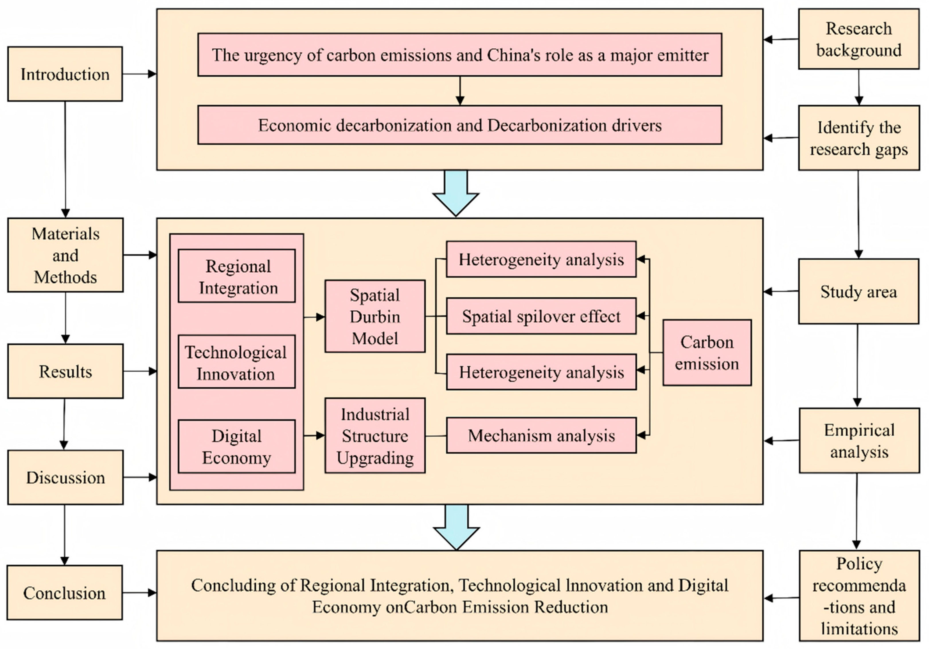
4.1. Spatiotemporal Evolution Patterns of Decarbonization Drivers

Since the 21st century, carbon emission pressures have emerged as a critical challenge for developing nations, with China confronting analogous issues. While the country achieved rapid economic growth following its reform and opening-up policy, the extensive development model led to technological stagnation in production, the overexploitation of resources, and environmental degradation. Since 2007, the central government has promoted regional economic and ecological integration, implementing a series of policies to build a “Resource-saving and Environment-friendly Society”, to alleviate emission reduction pressures. This study reveals that the carbon abatement effect of RI exhibits “short-term effectiveness but long-term limitations”, partially aligning with the inverted-U-shaped hypothesis identified by Zhang et al. [
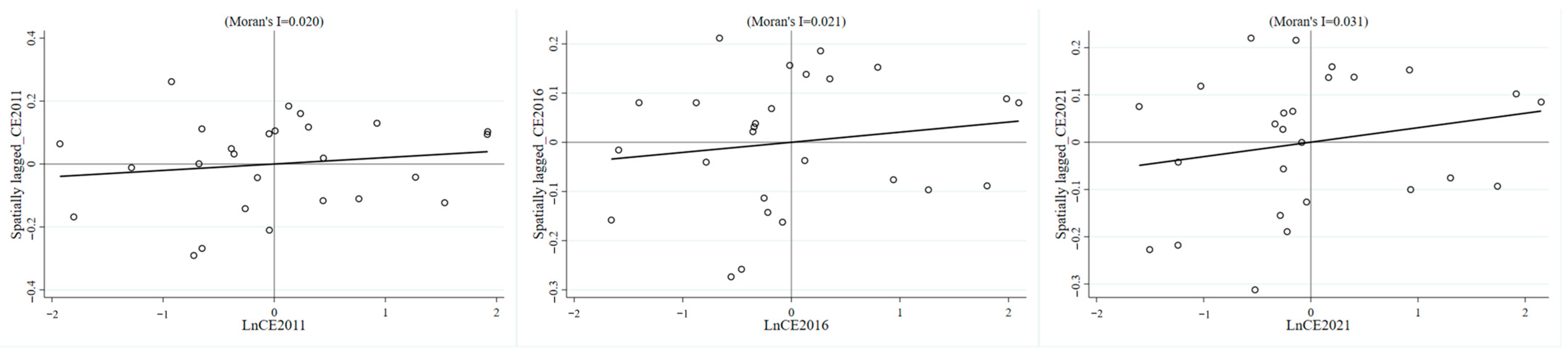
62]. The baseline regression results confirm its direct emission reduction effects, demonstrating that policy-driven resource integration facilitates decarbonization. RI provides a favorable environment for economically active and densely populated areas, facilitating the formation of economies of scale, enhancing enterprises’ capabilities to develop low-carbon technologies [63,64], and eliminating regional barriers to accelerate the diffusion of green technologies and management experiences [65]. It encourages the utilization of comparative advantages under market competition and influences carbon emissions by fostering innovation networks [66]. Notably, the YRD region has dedicated itself to ecologically friendly integrated development. By improving the convenience and sharing of public services, the government has enhanced public welfare and guided the adoption of green lifestyles. Environmental greening and governance have promoted green investment and consumption, while prioritizing public education has nurtured talent with sustainable development mindsets. Moreover, the spatial analysis reveals negligible and statistically insignificant spatial spillover effects from RI. This may stem from persistent administrative barriers and market fragmentation, coupled with divergent understandings and implementation approaches toward urban sustainability among local governments. Temporally, its long-term carbon reduction effect is weaker than its short-term impact. As integration progresses, an industrial structure lock-in effect may emerge, where energy-intensive industries form stable regional supply chains, weakening long-term emission reduction outcomes. In conclusion, the long-term development of RI is influenced by multiple factors [67], and its sustained effectiveness depends on incorporating more ecological elements.
TI plays a pivotal role in accelerating green economic transitions. This study reveals that the spatiotemporal evolution of TI follows a “short-term cost versus long-term dividend” pattern. Although green innovation technologies are widely regarded as core decarbonization drivers [68] capable of reducing emissions through production mode transformation and energy structure optimization [69,70,71], our empirical results show that TI initially increases local carbon emissions through direct effects. Initial technological investment is often accompanied by the “inertial expansion” of traditional industries. This paradoxical outcome may stem from productivity expansion in traditional industries prioritizing economic output over ecological efficiency [72], inadequate infrastructure for green technology adoption, and high costs of green innovation implementation triggering carbon rebound effects [73], suggesting a time-lagged decarbonization impact of technological innovation. However, further analysis demonstrates TI’s substantially stronger long-term decarbonization potential and enhanced spatial spillover effects. Over extended periods, green technological innovation facilitates the growth of digital finance industries to achieve emission reduction–economic growth dual objectives [54], while generating knowledge externalities that reduce cross-regional technology adoption costs through R&D spillovers. Inter-regional knowledge diffusion via labor mobility and corporate partnerships, particularly from high-R&D regions, enables broader technological dissemination. This evidence underscores the urgency to establish regional green technology trading platforms by leveraging patent sharing and joint R&D programs to dismantle innovation silos.
In China, DIE has emerged as a dynamic economic paradigm, flourishing alongside deepening RI and waves of TI. Unlike traditional systems reliant on massive fossil fuel consumption, DIE operates as a green, sustainable decarbonization driver [45], potentially catalyzing the decoupling of economic growth from carbon emissions [74,75]. This study confirms that DIE’s emission reduction capacity strengthens with enhanced spatial coordination. While it initially increases local carbon emissions through short-term direct effects, DIE demonstrates a significant long-term decarbonization potential and suppresses neighboring cities’ emissions via negative spatial spillovers. Furthermore, there is a certain synergy between DIE and TI. DIE is highly dependent on TI, but the adoption and scaling of technology require a maturation period. In the early stage of its integration with traditional industries, it may trigger a “scale paradox”: on the one hand, the digital transformation of enterprises requires the deployment of a large number of hardware facilities such as servers and communication equipment, whose manufacturing and operation generate direct carbon emissions; on the other hand, the empowerment of traditional industries by digital technology may stimulate capacity expansion in the short term, such as e-commerce driving the growth of logistics and freight volume, indirectly pushing up energy demand. In the absence of renewed energy from intensive R&D activities [76] and energy efficiency improvements from green technological innovations, DIE will lead to an undesirable increase in the output of traditional industrial products, instead promoting carbon emissions. The fact that the coefficient of DIE on carbon emissions is higher than that of TI in the direct effect results also confirms this point. This result is consistent with the “spatial imbalance” observation of Gu et al. [77], and further points out that the digital economy can strengthen the spatial spillover of technological innovation through the “learning effect”, effectively promoting carbon emission reduction. Similarly, its “learning effect” depends on infrastructure and policy support. Without green innovation support, it is likely to become a tool for the expansion of traditional industries. Therefore, policies should promote the “bundled” investment in digital infrastructure and green technologies.
These findings provide us with more insights. TI and DIE are more advanced decarbonization driving forces, and their improvement in urban energy and economic structure needs constant attention. Carbon reduction requires the market to provide a new low-carbon economic transition, rather than relying solely on the government’s master plan for the region. For example, due to the constraints of urban spatial planning, there is a saturation value for public services and urban greening, which weakens public contribution to low-carbon actions, and the physiological activities of biological sources increase carbon emissions [78].

4.2. Heterogeneity of Decarbonization Effects

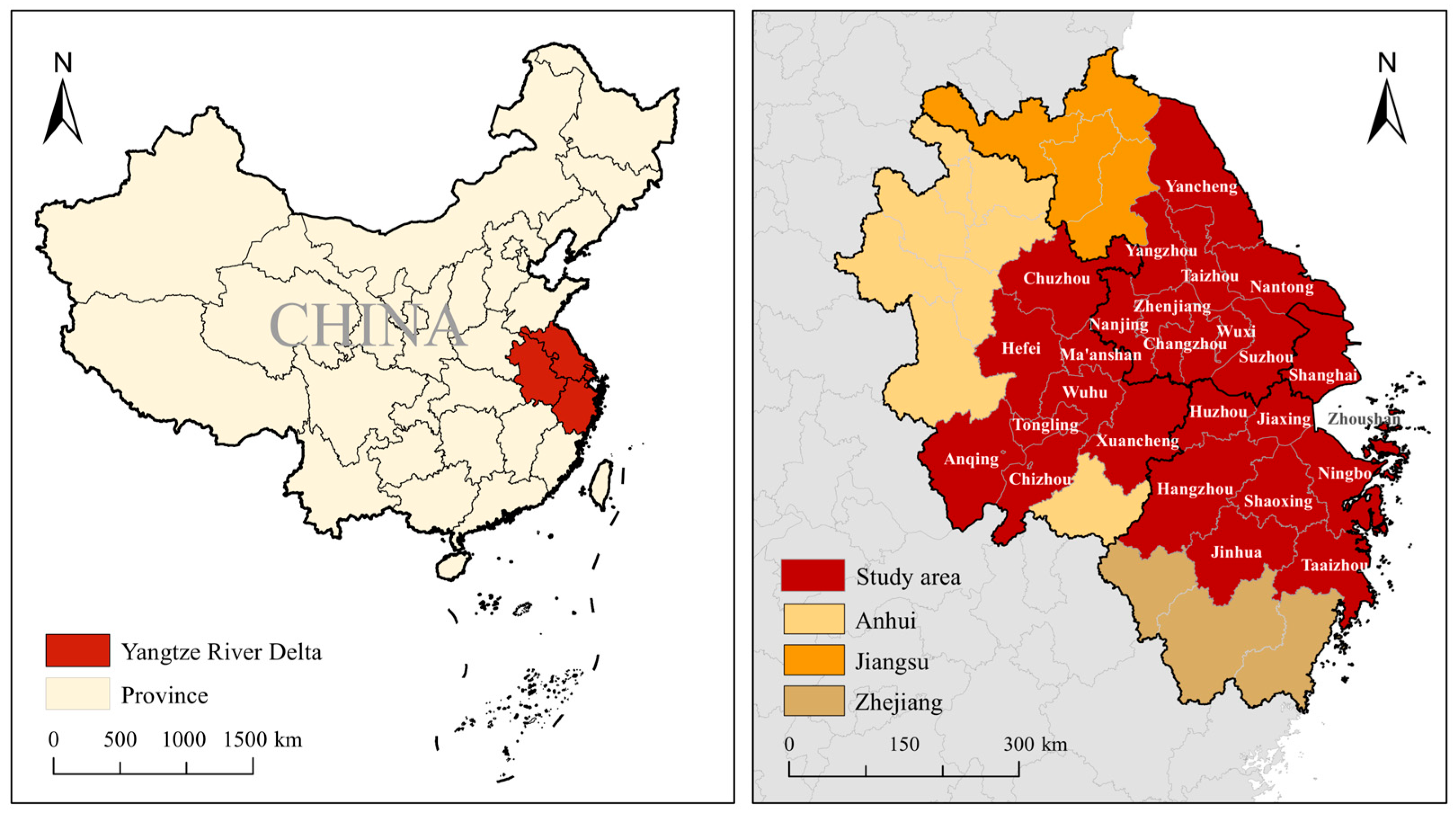
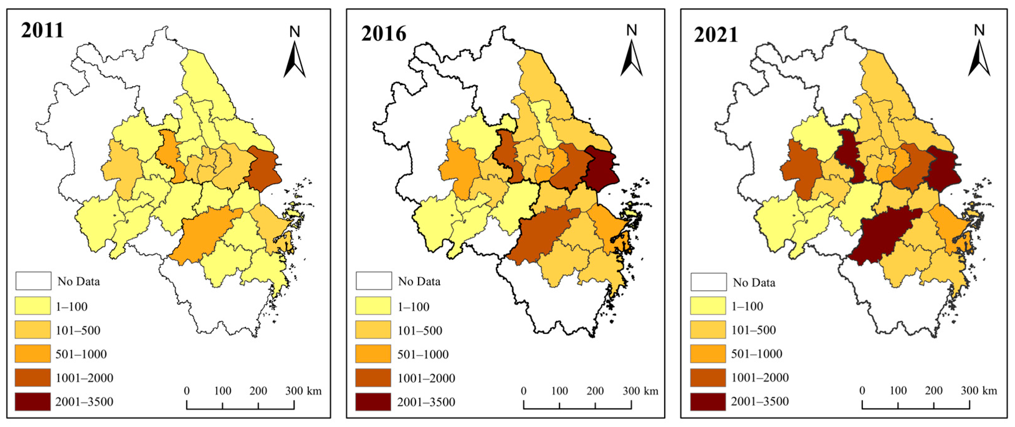
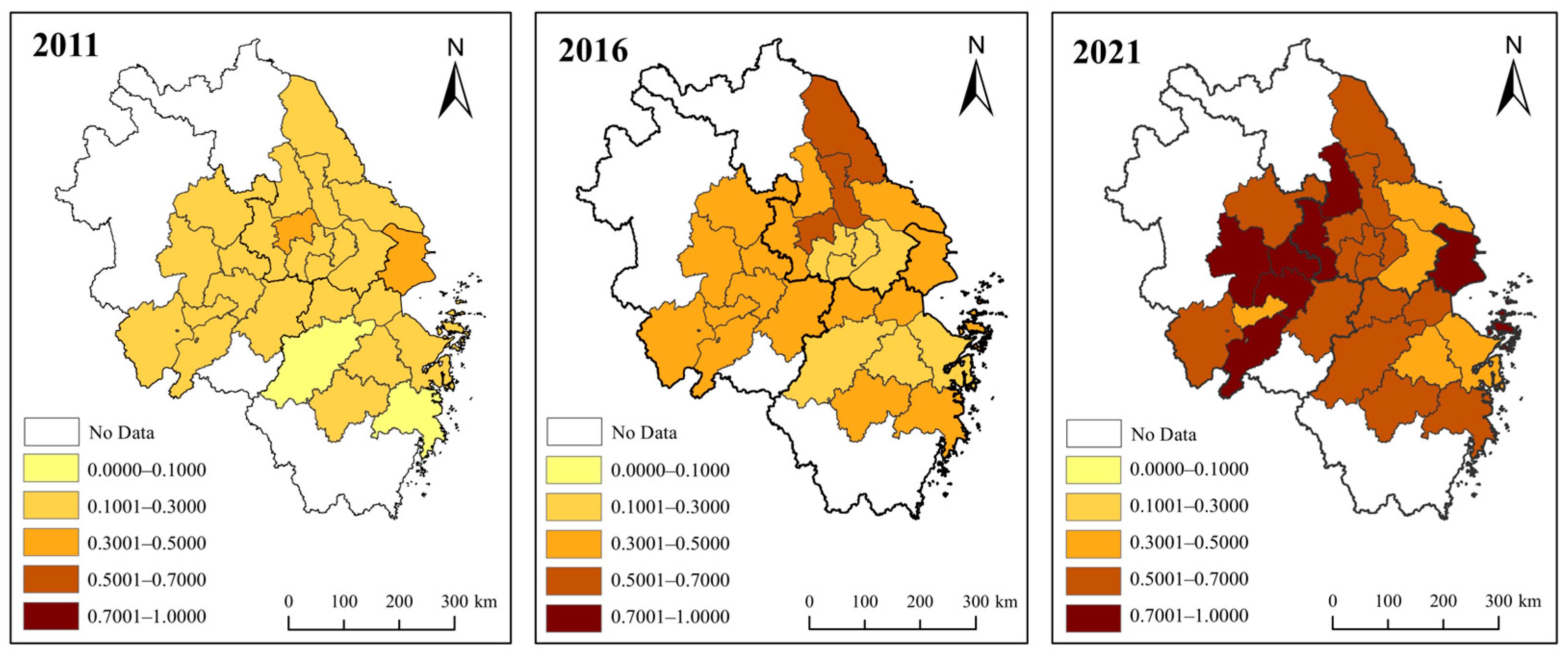
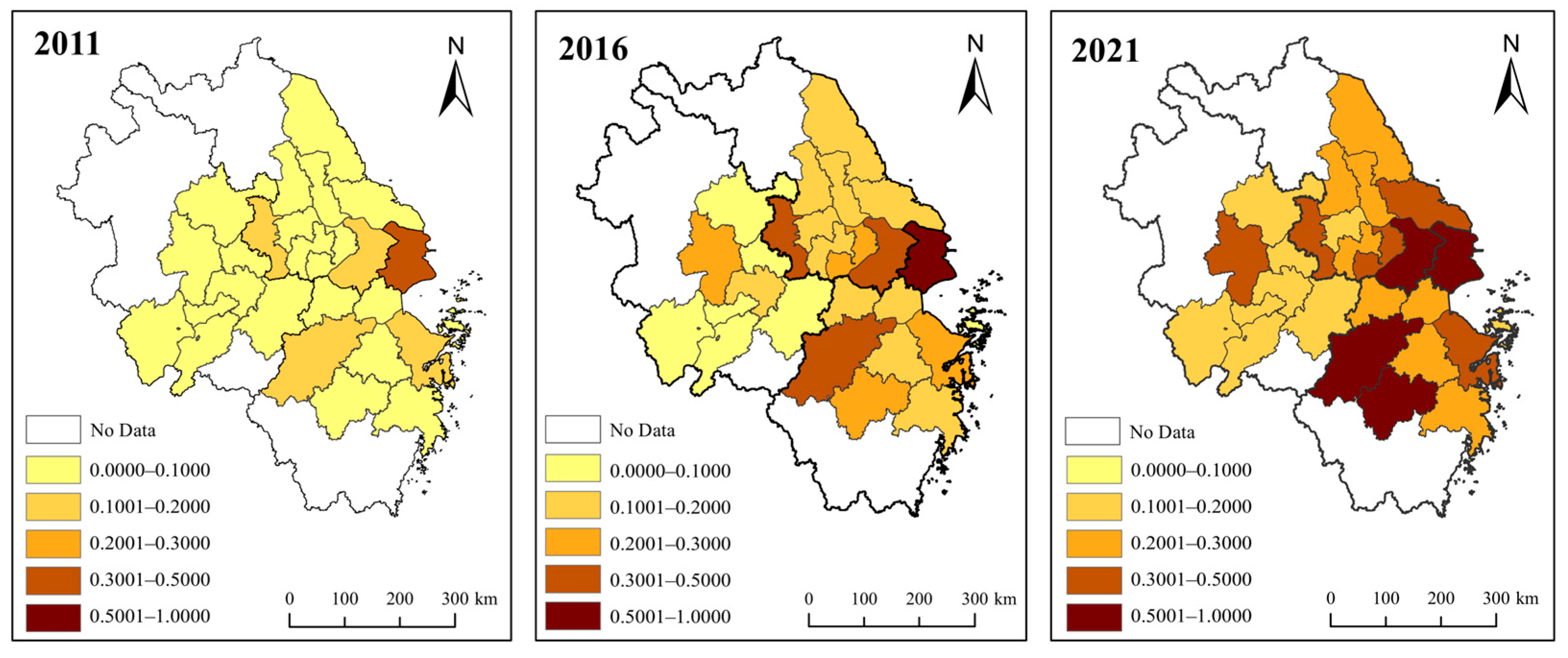
The findings of this study exhibit significant heterogeneity based on the characteristics of urban development time, economic differences, and energy structures. Firstly, the temporal heterogeneity analysis reveals that RI initially increases urban carbon emissions. After the 19th National Congress of the Communist Party of China in 2017, cities in the YRD were influenced by policies promoting regional coordinated development. The enhanced regional cooperation led to increased energy demand, which, to some extent, resulted in higher urban carbon emissions. Additionally, following the implementation of relevant policies, high-pollution industries were transferred. Environmental pollution in the YRD’s central cities decreased, while that in the peripheral cities increased, potentially leading to an overall rise in the environmental pollution level [79]. This further demonstrates the complexity of RI’s impact on carbon emissions: depending on government policies, pollutants, and the selection of research areas, the decarbonization effect of RI may yield opposite results [67]. Guided by the “Digital China” policy, the emission-reducing effects of TI and DIE gradually emerged, and the three decarbonization drivers showed opposite impact characteristics. After 2017, cities in the YRD paid more attention to achieving their ecological construction goals through the development of DIE and a new round of technological revolution. However, competition among local governments was evident. The actions of neighboring cities to promote RI can improve the regional integration framework of the local city and lead to a greater focus on ecological benefits. Nevertheless, it is difficult to find a more appropriate synergy between TI and DIE in mitigating climate change and reduce carbon emissions.
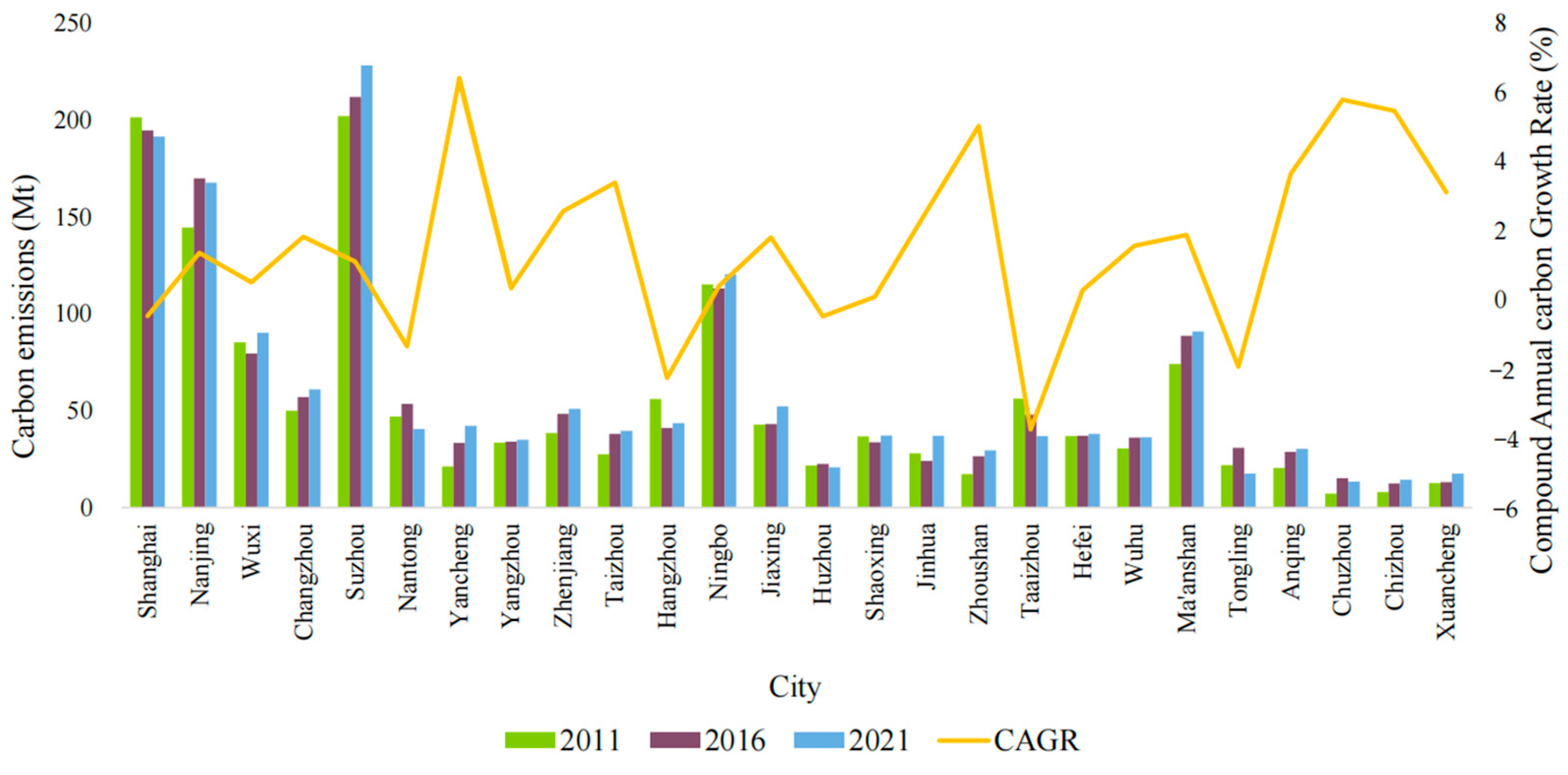
Secondly, regarding the decarbonization performance of different city types, economically advanced cities demonstrate a greater capacity to achieve “dual carbon” goals, while energy-intensive cities are held back by their traditional energy structures. Economically developed cities (such as Shanghai and Hangzhou) have sufficient capital investment and strong technology absorption capabilities, making it easier for them to leverage their capital and technology advantages to unleash their decarbonization potential. However, there are few ways to further expand this effect. The decarbonization effects of energy-intensive cities (such as Xuzhou and Ma’anshan) are severely restricted by their traditional energy structures. Such cities need to prioritize the transformation of their energy structures rather than blindly pursue the expansion of DIE. This finding confirms the impact of economic development levels and energy structures on carbon emissions [80] and further refines the analysis of differences among different city types in the decarbonization process. Policy formulation needs to be tailored to local conditions, and differentiated emission-reducing strategies should be formulated according to the characteristics of different cities.

4.3. Transmission Mechanisms of Industrial Structure Upgrading

The mechanism analysis reveals that UIS serves as a critical mediating mechanism through which TI and DIE influence carbon emissions. These findings confirm the importance of industrial structure adjustment in achieving low-carbon development [81]. However, UIS in YRD cities has not fully harnessed its emission reduction potential. As it only partially explains the decarbonization effects of TI and DIE, underlying mechanisms likely exist. This may stem from current industrial upgrading focusing predominantly on expanding the service-sector scale rather than fostering deep green technology penetration. Energy consumption growth in digital industries such as e-commerce and cloud computing partially offsets the benefits of industrial transformation [51,82]. Green technologies may be preferentially adopted in high-value-added sectors like semiconductor manufacturing, where energy consumption has not significantly decreased in the short term. Digital technologies can directly optimize energy use through smart grids and industrial IoT, operating independently of industrial structure changes. This finding provides a more targeted direction for future research and policy design. TI- and DIE-driven industries should avoid unsustainable development in low-end industrialization to prevent triggering a vicious cycle of environmental and economic decline. Emphasizing the goal of decarbonized development through UIS can foster the healthy development of decarbonization drivers.

4.4. Policy Recommendations and Limitations

It can be concluded that the development direction of economic decarbonization is consistent with the evolution trend of decarbonization driving forces. This means that the integration of traditional elements and policy incentives no longer dominates the process of carbon reduction but is replaced by active low-carbon technology applications and economic forms that can improve green growth rates. In light of these findings, several recommendations may be worth considering for policymakers: (1) To cultivate a conducive decarbonization environment for RI, market segregation and administrative barriers need to be removed from institutional mechanisms. Promoting the convenient sharing of public services in various fields and upgrading infrastructure conditions are also beneficial for the decarbonization effect of RI. For example, establishing a regularized information-sharing platform to disseminate timely information on policy dynamics and industrial development in the region, strengthen cooperation and communication among governments, and promote scientific and synergistic government decision-making. In respect of public services and infrastructure, new energy vehicle sharing services should be promoted, new energy vehicle leasing outlets should be increased, etc. More importantly, cities should bolster cooperative ecological environment preservation and administration so as to establish a green development base for RI. For instance, a cross-regional cooperation mechanism should be established for ecological protection and restoration projects and large-scale ecological restoration projects should be jointly carried out. Pollutant emission standards and treatment measures should be harmonized, and the development of clean energy should be promoted. A comprehensive carbon emissions trading system should be established. Low-carbon industries should be encouraged to become stronger and better. (2) Economic decarbonization cannot rely solely on the integration of traditional production factors and the improvement of resource allocation efficiency, but it needs to find long-term, competitive decarbonization driving forces. It is essential to integrate high-quality development elements like green TI and DIE across regions and sectors to serve the needs of “dual carbon” goals. For instance, this could be achieved by encouraging universities, research institutions, and enterprises to jointly carry out research on green technology innovation and promoting the application of digital technology in energy management, intelligent manufacturing, and other fields. For energy supply-intensive cities, it is recommended to implement targeted subsidies for green patents. For example, special funds should be established to support the transformation of patents related to clean coal utilization and industrial carbon capture technologies. The construction of a green patent sharing alliance in the YRD region should be promoted, allowing energy-intensive cities to obtain free access to the patent rights of core cities. Importantly, the government should establish a “non-zero-sum game” concept to synergistically develop and promote the positive spillover effects of green TI and DIE and avoid the regional “carbon leakage” phenomenon caused by the transfer of polluting industries. Establishing an environmental assessment mechanism for regional industrial transfers should be considered, and rigorous carbon emission assessments of industrial projects to be transferred should be conducted. In addition, UIS is a positive way to cultivate decarbonization potential. (3) Carbon emission reduction strategies in cities should be oriented toward sustainable development, follow the pattern of economic decarbonization, and reasonably formulate emission reduction targets and policy initiatives based on the heterogeneity of decarbonization driving forces in cities. Urban development should focus on synchronizing economic and ecological benefits. Cities at a disadvantage in RI should mobilize green production and consumption initiatives, aim for long-term carbon neutrality goals, introduce green technologies, and accelerate the creation and layout of low-carbon industrial development spaces. Specific measures include establishing citizen green consumption incentive mechanisms and setting up special funds for low-carbon technologies. A higher RI should be followed by a shift toward the exploration of emerging decarbonization technologies and economies. For example, to promote the sharing of advantageous resources such as emission-reducing and energy-saving technologies. Moreover, cities can support the digital and clean development of the energy industry, namely, by ensuring that the efficiency of the energy supply does not decline and by accelerating the low-carbon transition of the energy mix.
Finally, it is acknowledged that this article still faces some limitations. First, although this study made significant efforts to explore the evolution and effects of important drivers of decarbonization separately, according to urban development, it still could not address the specific limitations regarding coupled carbon reduction. Future research could further investigate the meaningful impacts from the coupled coordination theory perspective using more appropriate modeling and extend future research by delving into the interaction mechanisms between RI, TI, and DIE. Second, the time span of this study is only up to 2021, so the sample survey time should be updated and extended into the future to bring more current and relevant results to the study. The research method is mainly quantitative analysis, lacking a qualitative discussion of the details of policy implementation. Additionally, applying the theoretical framework or model to more urban agglomerations is necessary to assess its applicability and generalizability. Third, within the constraints of space and different research focuses, future research could also examine the impact of urban water pollution and solid waste management on carbon emissions. Other drivers from different perspectives are present, such as the direction of TI in the industry, the type of digitization, and the allocation and pricing of land, which can also affect decarbonization. This paper only explores UIS as the core mediating mechanism, without addressing diversified transmission pathways such as green finance, circular economy practices, or public behavior changes. Future research could consider incorporating these factors and conducting in-depth analyses to obtain a more comprehensive understanding of the decarbonization process. Nonetheless, this paper provides robust empirical results as well as some valuable insights and enhances confidence in the study of the driving forces of economic decarbonization.

5. Conclusions

Economic decarbonization is a major strategic arrangement that China is and will firmly be determined to promote. Under the vision of “dual carbon” goals, urban agglomerations are key implementation units for realizing these. RI, TI, and DIE have become key decarbonization drivers. This paper primarily utilizes spatial econometric models to examine their respective relationships with urban carbon emissions while attempting to elucidate the evolution patterns of their decarbonization capabilities. Furthermore, this paper offers more comprehensive evidence from the perspectives of heterogeneity and intrinsic mechanisms. In summary, the following conclusions have been drawn: (1) RI, TI, and DIE are spatially connected in terms of their influence on urban carbon emissions and contribute to the economic decarbonization of the YRD. (2) Population growth and traditional energy supply structures are major obstacles to achieving net-zero emissions. TI and DIE exhibit stronger spatial spillover effects, and both are expected to unlock greater decarbonization potential in the long run. (3) RI, TI, and DIE, as driving forces for decarbonization, follow a certain evolutionary pattern. In the short term, RI is more effective in reducing emissions, while the long-term impact hinges on integrating more ecological elements. DIE tends to expand the decarbonization capacity of RI and TI chronically, but this expansion should be predicated on a commitment to the widespread application of low-carbon technologies in the industrial sectors within the area. (4) The temporal heterogeneity shows that TI and DIE demonstrated significant emission reduction effects after 2017. Cities in the YRD region that are relatively economically developed are more capable of realizing “dual carbon” goals, while energy-intensive cities are being dragged down by traditional energy structures. (5) The transmission mechanism is indispensable in studying the impact of TI and DIE on carbon emissions. Through the mediating pathway of UIS, carbon emissions will ultimately be suppressed.

Author Contributions

Conceptualization, H.W.; formal analysis, X.S.; funding acquisition, H.W.; investigation, X.L.; methodology, X.S.; software, X.S.; supervision, H.W.; validation, X.S.; writing—original draft, X.S.; writing—review and editing, X.L. All authors have read and agreed to the published version of the manuscript.

Funding

This research was funded by the Planning Fund of the Ministry of Education, Humanities and Social Sciences of China [No. 22YJA630096].

Institutional Review Board Statement

Not applicable.

Informed Consent Statement

Not applicable.

Data Availability Statement

Publicly available datasets were analyzed in this study. The data were from China Emission Accounts and Datasets (CEADs), China Stock Market & Accounting Research Database (CSMAR), Chinese Research Data Services Platform, and China City Greenhouse Gas Working Group.

Acknowledgments

Thanks to the anonymous reviewers and all the editors in the process of revision.

Conflicts of Interest

The authors declare no conflicts of interest.

References

  1. DeConto, R.M.; Pollard, D.; Alley, R.B.; Velicogna, I.; Gasson, E.; Gomez, N.; Sadai, S.; Condron, A.; Gilford, D.M.; Ashe, E.L.; et al. The Paris Climate Agreement and Future Sea-Level Rise from Antarctica. Nature 2021, 593, 83–89. [Google Scholar] [CrossRef] [PubMed]
  2. Sala, S.; Crenna, E.; Secchi, M.; Sanyé-Mengual, E. Environmental Sustainability of European Production and Consumption Assessed against Planetary Boundaries. J. Environ. Manag. 2020, 269, 110686. [Google Scholar] [CrossRef] [PubMed]
  3. Chen, J.D.; Wang, P.; Cui, L.B.; Huang, S.; Song, M.L. Decomposition and Decoupling Analysis of CO2 Emissions in OECD. Appl. Energy 2018, 231, 937–950. [Google Scholar] [CrossRef]
  4. Lee, C.-C.; He, Z.-W. Natural Resources and Green Economic Growth: An Analysis Based on Heterogeneous Growth Paths. Resour. Policy 2022, 79, 103006. [Google Scholar] [CrossRef]
  5. Liu, J.Y.; Murshed, M.; Chen, F.Z.; Shahbaz, M.; Kirikkaleli, D.; Khan, Z. An Empirical Analysis of the Household Consumption-Induced Carbon Emissions in China. Sustain. Prod. Consum. 2021, 26, 943–957. [Google Scholar] [CrossRef]
  6. Su, W.H.; Zhang, D.C.; Zhang, C.H.; Streimikiene, D. Sustainability Assessment of Energy Sector Development in China and European Union. Sustain. Dev. 2020, 28, 1063–1076. [Google Scholar] [CrossRef]
  7. CCG. China City Carbon Dioxide Emissions Dataset. 2022. Available online: http://www.cityghg.com/toCauses?id=4 (accessed on 7 October 2024).
  8. BP. Statistical Review of World Energy. 2021. Available online: https://www.bp.com/content/dam/bp/business-sites/en/global/corporate/pdfs/energy-economics/statistical-review/bp-stats-review-2021-full-report.pdf (accessed on 7 October 2024).
  9. NDRC. Indicator 4 in the Outline of the 14th Five-Year Plan: Proportion of Non-Fossil Energy in Total Energy Consumption. 2021. Available online: https://www.ndrc.gov.cn/fggz/fzzlgh/gjfzgh/202112/t20211225_1309671.html (accessed on 29 May 2025).
  10. Zhou, X.Y.; Zhang, J.; Li, J.P. Industrial Structural Transformation and Carbon Dioxide Emissions in China. Energy Policy 2013, 57, 43–51. [Google Scholar] [CrossRef]
  11. Li, X.J.; Lin, C.X.; Lin, M.C.; Jim, C.Y. Drivers, Scenario Prediction and Policy Simulation of the Carbon Emission System in Fujian Province (China). J. Clean. Prod. 2024, 434, 140375. [Google Scholar] [CrossRef]
  12. Wang, P.; Wu, W.S.; Zhu, B.Z.; Wei, Y.M. Examining the Impact Factors of Energy-Related CO2 Emissions Using the STIRPAT Model in Guangdong Province, China. Appl. Energy 2013, 106, 65–71. [Google Scholar] [CrossRef]
  13. Guo, W.; Sun, T.; Dai, H.J. Effect of Population Structure Change on Carbon Emission in China. Sustainability 2016, 8, 225. [Google Scholar] [CrossRef]
  14. Wang, Q.; Li, L.J. The Effects of Population Aging, Life Expectancy, Unemployment Rate, Population Density, per Capita GDP, Urbanization on per Capita Carbon Emissions. Sustain. Prod. Consum. 2021, 28, 760–774. [Google Scholar] [CrossRef]
  15. Meng, L.; Guo, J.; Chai, J.; Zhang, Z.K. China’s Regional CO2 Emissions: Characteristics, Inter-Regional Transfer and Emission Reduction Policies. Energy Policy 2011, 39, 6136–6144. [Google Scholar] [CrossRef]
  16. Shahbaz, M.; Loganathan, N.; Muzaffar, A.T.; Ahmed, K.; Jabran, M.A. How Urbanization Affects CO2 Emissions of STIRPAT Model in Malaysia? The Application. Renew. Sustain. Energy Rev. 2016, 57, 83–93. [Google Scholar] [CrossRef]
  17. Millimet, D.L.; Roy, J. Empirical Tests of the Pollution Haven Hypothesis When Environmental Regulation Is Endogenous. J. Appl. Economet. 2016, 31, 652–677. [Google Scholar] [CrossRef]
  18. Chen, Y.; Shao, S.; Fan, M.T.; Tian, Z.H.; Yang, L.L. One Man’s Loss Is Another’s Gain: Does Clean Energy Development Reduce CO2 Emissions in China? Evidence Based on the Spatial Durbin Model. Energy Econ. 2022, 107, 105852. [Google Scholar] [CrossRef]
  19. Lin, B.Q.; Zhu, J.P. Impact of China’s New-Type Urbanization on Energy Intensity: A City-Level Analysis. Energy Econ. 2021, 99, 105292. [Google Scholar] [CrossRef]
  20. Zhang, H.; Feng, C.; Zhou, X.X. Going Carbon-Neutral in China: Does the Low-Carbon City Pilot Policy Improve Carbon Emission Efficiency? Sustain. Prod. Consum. 2022, 33, 312–329. [Google Scholar] [CrossRef]
  21. Zhang, A.L.; Wen, L.J.; Chatalova, L.; Gao, X. Reduction of Carbon Emissions through Resource-Saving and Environment-Friendly Regional Economic Integration: Evidence from Wuhan Metropolitan Area, China. Technol. Forecast. Soc. 2021, 166, 120590. [Google Scholar] [CrossRef]
  22. Pei, Y.; Zhu, Y.M.; Liu, S.X.; Wang, X.C.; Cao, J.J. Environmental Regulation and Carbon Emission: The Mediation Effect of Technical Efficiency. J. Clean. Prod. 2019, 236, 117599. [Google Scholar] [CrossRef]
  23. Ren, H.J.; Zhao, J.B. The Impact of technological innovation and structural adjustment on energy consumption: A PVAR empirical analysis based on carbon emission grouping. Soft Sci. 2018, 32, 30–34. [Google Scholar] [CrossRef]
  24. Zhu, X.W. Have Carbon Emissions Been Reduced Due to the Upgrading of Industrial Structure? Analysis of the Mediating Effect Based on Technological Innovation. Environ. Sci. Pollut. Res. 2022, 29, 54890–54901. [Google Scholar] [CrossRef] [PubMed]
  25. Li, Z.G.; Wang, J. The Dynamic Impact of Digital Economy on Carbon Emission Reduction: Evidence City-Level Empirical Data in China. J. Clean. Prod. 2022, 351, 131570. [Google Scholar] [CrossRef]
  26. Xu, Q.; Zhong, M.; Cao, M. Does Digital Investment Affect Carbon Efficiency? Spatial Effect and Mechanism Discussion. Sci. Total Environ. 2022, 827, 154321. [Google Scholar] [CrossRef]
  27. Yang, Z.; Gao, W.; Han, Q.; Qi, L.; Cui, Y.; Chen, Y. Digitalization and Carbon Emissions: How Does Digital City Construction Affect China’s Carbon Emission Reduction? Sustain. Cities Soc. 2022, 87, 104201. [Google Scholar] [CrossRef]
  28. NDRC. Yangtze River Delta City Cluster Development Plan. 2016. Available online: https://www.ndrc.gov.cn/xxgk/zcfb/ghwb/201606/t20160603_962187.html (accessed on 19 November 2024).
  29. Li, W.; Chen, Z.J.; Li, M.C.; Zhang, H.; Li, M.Y.; Qiu, X.Q.; Zhou, C. Carbon Emission and Economic Development Trade-Offs for Optimizing Land-Use Allocation in the Yangtze River Delta, China. Ecol. Indic. 2023, 147, 109950. [Google Scholar] [CrossRef]
  30. NBSC. 2022 China Statistical Yearbook. 2023. Available online: https://www.stats.gov.cn/sj/ndsj/2022/indexch.htm (accessed on 1 June 2025).
  31. Tikoudis, I.; Oueslati, W. The Future of Transport-Related Emissions in Dense Urban Areas: An Analysis of Various Policy Scenarios with MOLES. Environ. Econ. Pol. Stud. 2023, 25, 205–268. [Google Scholar] [CrossRef]
  32. Ye, C.; Zhu, J.J.; Li, S.M.; Yang, S.; Chen, M.X. Assessment and Analysis of Regional Economic Collaborative Development within an Urban Agglomeration: Yangtze River Delta as a Case Study. Habitat Int. 2019, 83, 20–29. [Google Scholar] [CrossRef]
  33. Yu, Q.Y.; Li, M.; Li, Q.; Wang, Y.N.; Chen, W. Economic Agglomeration and Emissions Reduction: Does High Agglomeration in China’s Urban Clusters Lead to Higher Carbon Intensity? Urban Clim. 2022, 43, 101174. [Google Scholar] [CrossRef]
  34. CAEP. The Yangtze River Delta Integration Development Plan. 2020. Available online: http://www.caep.org.cn/sy/sswhbgh/dt/202006/W020200628436948544560.pdf (accessed on 7 October 2024).
  35. CAICT. The Yangtze River Delta Digital Economy Development Report. 2021. Available online: http://www.caict.ac.cn/kxyj/qwfb/ztbg/202110/P020211008607517660797.pdf (accessed on 7 October 2024).
  36. Shan, Y.L.; Guan, D.B.; Liu, J.H.; Mi, Z.F.; Liu, Z.; Liu, J.R.; Schroeder, H.; Cai, B.F.; Chen, Y.; Shao, S.; et al. Methodology and Applications of City Level CO2 Emission Accounts in China. J. Clean. Prod. 2017, 161, 1215–1225. [Google Scholar] [CrossRef]
  37. Shan, Y.L.; Guan, D.B.; Klaus, H.; Zheng, B.; Steven, J.D.; Jia, L.C.; Liu, J.H.; Liu, Z.; Neil, F.; Mi, Z.F.; et al. City-Level Climate Change Mitigation in China. Sci. Adv. 2018, 4, eaaq0390. [Google Scholar] [CrossRef]
  38. Shan, Y.L.; Liu, J.H.; Liu, Z.; Shao, S.; Guan, D.B. An Emissions-Socioeconomic Inventory of Chinese Cities. Sci. Data 2019, 6, 190027. [Google Scholar] [CrossRef] [PubMed]
  39. Shan, Y.L.; Guan, Y.R.; Hang, Y.; Zheng, H.R.; Li, Y.X.; Guan, D.; Li, J.; Zhou, Y.; Li, L.; Hubacek, K. City-Level Emission Peak and Drivers in China. Sci. Bull. 2022, 67, 1910–1920. [Google Scholar] [CrossRef]
  40. Zhang, W.; Liu, X.M.; Wang, D.; Zhou, J.P. Digital Economy and Carbon Emission Performance: Evidence at China’s City Level. Energy Policy 2022, 165, 112927. [Google Scholar] [CrossRef]
  41. Chen, S.Y.; Tan, Z.X.; Mu, S.Y.; Wang, J.Y.; Chen, Y.Y.; He, X.W. Synergy Level of Pollution and Carbon Reduction in the Yangtze River Economic Belt: Spatial-Temporal Evolution Characteristics and Driving Factors. Sustain. Cities Soc. 2023, 98, 104859. [Google Scholar] [CrossRef]
  42. Chen, X.L.; Di, Q.B.; Jia, W.H.; Hou, Z.W. Spatial Correlation Network of Pollution and Carbon Emission Reductions Coupled with High-Quality Economic Development in Three Chinese Urban Agglomerations. Sustain. Cities Soc. 2023, 94, 104552. [Google Scholar] [CrossRef]
  43. Chen, D.L.; Hu, W.B.; Li, Y.Y.; Zhang, C.Z.; Lu, X.H.; Cheng, H. Exploring the Temporal and Spatial Effects of City Size on Regional Economic Integration: Evidence from the Yangtze River Economic Belt in China. Land Use Policy 2023, 132, 106770. [Google Scholar] [CrossRef]
  44. Zhang, W.S.; Xu, Y.; Streets, D.G.; Wang, C. Can New-Type Urbanization Realize Low-Carbon Development? A Spatiotemporal Heterogeneous Analysis in 288 Cities and 18 Urban Agglomerations in China. J. Clean. Prod. 2023, 420, 138426. [Google Scholar] [CrossRef]
  45. Yi, M.; Liu, Y.F.; Sheng, M.S.; Wen, L. Effects of Digital Economy on Carbon Emission Reduction: New Evidence from China. Energy Policy 2022, 171, 113271. [Google Scholar] [CrossRef]
  46. Xiao, Y.; Zhong, J.L.; Zhang, Q.F.; Xiang, X.; Huang, H. Exploring the Coupling Coordination and Key Factors between Urbanization and Land Use Efficiency in Ecologically Sensitive Areas: A Case Study of the Loess Plateau, China. Sustain. Cities Soc. 2022, 86, 104148. [Google Scholar] [CrossRef]
  47. Feng, Y.; Sun, M.; Pan, Y.; Zhang, C. Fostering Inclusive Green Growth in China: Identifying the Impact of the Regional Integration Strategy of Yangtze River Economic Belt. J. Environ. Manag. 2024, 358, 120952. [Google Scholar] [CrossRef]
  48. Zhang, H.J.; Zhang, Z.M. Financial opening, industrial structure upgrading and economic integration development: An Empirical Study Based on the Yangtze River Delta urban agglomeration. Econ. Issues Explor. 2020, 5, 122–133. [Google Scholar]
  49. Sun, G.; Fang, J.; Li, J.; Wang, X. Research on the Impact of the Integration of Digital Economy and Real Economy on Enterprise Green Innovation. Technol. Forecast. Soc. 2024, 200, 123097. [Google Scholar] [CrossRef]
  50. Wang, J.D.; Dong, X.C.; Dong, K.Y. How Digital Industries Affect China’s Carbon Emissions? Analysis of the Direct and Indirect Structural Effects. Technol. Soc. 2022, 68, 101911. [Google Scholar] [CrossRef]
  51. Zhang, L.; Mu, R.Y.; Zhan, Y.F.; Yu, J.H.; Liu, L.Y.; Yu, Y.S.; Zhang, J.X. Digital Economy, Energy Efficiency, and Carbon Emissions: Evidence from Provincial Panel Data in China. Sci. Total Environ. 2022, 852, 158403. [Google Scholar] [CrossRef]
  52. Bai, L.; Guo, T.R.; Xu, W.; Liu, Y.M.; Kuang, M.; Jiang, L. Effects of Digital Economy on Carbon Emission Intensity in Chinese Cities: A Life-Cycle Theory and the Application of Non-Linear Spatial Panel Smooth Transition Threshold Model. Energy Policy 2023, 183, 113792. [Google Scholar] [CrossRef]
  53. Bai, T.T.; Qi, Y.; Li, Z.H.; Xu, D. Digital Economy, Industrial Transformation and Upgrading, and Spatial Transfer of Carbon Emissions: The Paths for Low-Carbon Transformation of Chinese Cities. J. Environ. Manag. 2023, 344, 118528. [Google Scholar] [CrossRef] [PubMed]
  54. Song, X.L.; Yao, Y.M.; Wu, X.K. Digital Finance, Technological Innovation, and Carbon Dioxide Emissions. Econ. Anal. Policy 2023, 80, 482–494. [Google Scholar] [CrossRef]
  55. Wu, L.F.; Sun, L.W.; Qi, P.X.; Ren, X.W.; Sun, X.T. Energy Endowment, Industrial Structure Upgrading, and CO2 Emissions in China: Revisiting Resource Curse in the Context of Carbon Emissions. Resour. Pol. 2021, 74, 102329. [Google Scholar] [CrossRef]
  56. CSMAR. China Stock Market & Accounting Research Database. 2022. Available online: https://data.csmar.com/ (accessed on 6 October 2024).
  57. CEADs. China Emission Accounts and Datasets. 2022. Available online: https://www.ceads.net.cn/ (accessed on 6 October 2024).
  58. CNRDS. Chinese Research Data Services. 2022. Available online: https://www.cnrds.com/ (accessed on 6 October 2024).
  59. Elhorst, J.P. Matlab Software for Spatial Panels. Int. Reg. Sci. Rev. 2014, 37, 389–405. [Google Scholar] [CrossRef]
  60. Guo, B.S.; He, D.W.; Jin, G. Agricultural Production Efficiency Estimation and Spatiotemporal Convergence Characteristic Analysis in the Yangtze River Economic Belt: A Semi-Parametric Metafrontier Approach. Land Degrad. Dev. 2023, 34, 4635–4648. [Google Scholar] [CrossRef]
  61. Baron, R.M.; Kenny, D.A. The Moderator–Mediator Variable Distinction in Social Psychological Research: Conceptual, Strategic, and Statistical Considerations. J. Pers. Soc. Psychol. 1986, 51, 1173–1182. [Google Scholar] [CrossRef] [PubMed]
  62. Zhang, K.; Shao, S.; Fan, S.Y. Market Integration and Environmental Quality: Evidence from the Yangtze River Delta Region of China. J. Environ. Manag. 2020, 261, 110208. [Google Scholar] [CrossRef]
  63. Tybout, J.R. Manufacturing Firms in Developing Countries: How Well Do They Do, and Why? J. Econ. Lit. 2000, 38, 11–44. [Google Scholar] [CrossRef]
  64. Van Biesebroeck, J. Exporting Raises Productivity in Sub-Saharan African Manufacturing Firms. J. Int. Econ. 2005, 67, 373–391. [Google Scholar] [CrossRef]
  65. Peluffo, A. Regional Integration and Technology Diffusion: The Case of Uruguay. J. Int. Trade Econ. Dev. 2013, 22, 786–816. [Google Scholar] [CrossRef]
  66. Grossman, G.M.; Helpman, E. Globalization and Growth. Amer. Econ. Rev. 2015, 105, 100–104. [Google Scholar] [CrossRef]
  67. Guo, Y.; Cao, X.Z.; Wei, W.D.; Ceng, G. The Impact of Regional Integration in the Yangtze River Delta on Urban Carbon Emissions. Geogr. Res. 2022, 41, 181–192. [Google Scholar] [CrossRef]
  68. Xu, L.; Fan, M.T.; Yang, L.L.; Shao, S. Heterogeneous Green Innovations and Carbon Emission Performance: Evidence at China’s City Level. Energy Econ. 2021, 99, 105269. [Google Scholar] [CrossRef]
  69. Gu, J.F. Sharing Economy, Technological Innovation and Carbon Emissions: Evidence from Chinese Cities. J. Innov. Knowl. 2022, 7, 100228. [Google Scholar] [CrossRef]
  70. Li, G.H.; Chen, X.; You, X.-Y. System Dynamics Prediction and Development Path Optimization of Regional Carbon Emissions: A Case Study of Tianjin. Renew. Sustain. Energy Rev. 2023, 184, 113579. [Google Scholar] [CrossRef]
  71. Huang, Y.M.; Wang, Y.; Peng, J.T.; Li, F.; Zhu, L.; Zhao, H.H.; Shi, R. Can China Achieve Its 2030 and 2060 CO2 Commitments? Scenario Analysis Based on the Integration of LEAP Model with LMDI Decomposition. Sci. Total Environ. 2023, 888, 164151. [Google Scholar] [CrossRef] [PubMed]
  72. Shao, S.; Chen, Y.; Li, K.; Yang, L.L. Market Segmentation and Urban CO2 Emissions in China: Evidence from the Yangtze River Delta Region. J. Environ. Manag. 2019, 248, 109324. [Google Scholar] [CrossRef] [PubMed]
  73. Liang, H.Y.; Lin, S.J.; Wang, J. Impact of Technological Innovation on Carbon Emissions in China’s Logistics Industry: Based on the Rebound Effect. J. Clean. Prod. 2022, 377, 134371. [Google Scholar] [CrossRef]
  74. Ma, Q.; Tariq, M.; Mahmood, H.; Khan, Z. The Nexus between Digital Economy and Carbon Dioxide Emissions in China: The Moderating Role of Investments in Research and Development. Technol. Soc. 2022, 68, 101910. [Google Scholar] [CrossRef]
  75. Zhao, X.; Ma, X.W.; Chen, B.Y.; Shang, Y.P.; Song, M.L. Challenges toward Carbon Neutrality in China: Strategies and Countermeasures. Resour. Conserv. Recycl. 2022, 176, 105959. [Google Scholar] [CrossRef]
  76. Saia, A. Digitalization and CO2 Emissions: Dynamics under R&D and Technology Innovation Regimes. Technol. Soc. 2023, 74, 102323. [Google Scholar] [CrossRef]
  77. Gu, R.D.; Li, C.F.; Yang, Y.Y.; Zhang, J. The Impact of Industrial Digital Transformation on Green Development Efficiency Considering the Threshold Effect of Regional Collaborative Innovation: Evidence from the Beijing-Tianjin-Hebei Urban Agglomeration in China. J. Clean. Prod. 2023, 420, 138345. [Google Scholar] [CrossRef]
  78. Hu, R.F.; Xu, W.Q.; Liu, L.-F.; Cui, Z.Y.; Zhao, C.Y. The Impact of Urban Agglomerations on Carbon Emissions in China: Spatial Scope and Mechanism. J. Clean. Prod. 2023, 419, 138250. [Google Scholar] [CrossRef]
  79. Lu, G.Y.; Zhang, B. Study on pollution heterogeneity of urban agglomeration in Yangtze River Delta. China Popul. Resour. Environ. 2020, 30, 110–117. [Google Scholar]
  80. Guo, Q.R.; Çoban, M.N.; Hossain, M.R.; Wu, Z.; Abbas, S.; Khudoykulov, K. Unveiling the Past, Shaping the Future: Analyzing Three Centuries of Data to Explore China’s Trajectory towards Carbon Neutrality. J. Clean. Prod. 2023, 420, 138348. [Google Scholar] [CrossRef]
  81. Zhang, K. Regional integration, environmental pollution and social welfare. J. Financ. Res. 2020, 486, 114–131. [Google Scholar]
  82. Zhou, X.Y.; Zhou, D.Q.; Wang, Q.W.; Su, B. How Information and Communication Technology Drives Carbon Emissions: A Sector-Level Analysis for China. Energy Econ. 2019, 81, 380–392. [Google Scholar] [CrossRef]
Figure 1. The main framework of the study.
Sustainability 17 05463 g001
Figure 2. Overview of the study area and distribution of sample cities.
Sustainability 17 05463 g002
Figure 3. The carbon emissions and compound annual carbon growth rate of cities in the YRD in 2011, 2016, and 2021.
Sustainability 17 05463 g003
Figure 4. Green invention patent authorizations for cities in the YRD from 2011 to 2021.
Sustainability 17 05463 g004
Figure 5. Spatiotemporal evolution of technological innovation of the cities in the YRD in 2011, 2016, and 2021.
Sustainability 17 05463 g005
Figure 6. Spatiotemporal evolution of regional integration of the cities in the YRD in 2011, 2016, and 2021.
Sustainability 17 05463 g006
Figure 7. Spatiotemporal evolution of the digital economy of the cities in the YRD in 2011, 2016, and 2021.
Sustainability 17 05463 g007
Figure 8. Moran’s scatter plots of carbon emissions with W 1 in 2011, 2016, and 2021.
Sustainability 17 05463 g008
Table 1. The measurement indicator system of the regional integration.
Primary DimensionSecondary IndicatorUnitIndicator AttributeReferences
Social life
stratification plane
Urban basic pension insurance participants104+[42]
Urban basic medical insurance participants104+[42]
Number of medical institutions-+[42]
Beds in medical institutions-+[42]
Average wage of full-time-employed workersCNY 104 +[42,43]
Domestic waste disposal rate%+[42]
Urban green coverage area104 m2+[40,41]
Total collection of public libraries104+[44]
College students per 10,000 people-+[20,45,46]
Proportion of education expenditure in GDP%+[42,47]
Economic life
stratification plane
Balance of financial institution loanCNY 108+[20,25]
Balance of financial institution depositCNY 108 +[25]
Total retail sales of consumer goodsCNY 108 +[42]
Highway passenger transport quantity104+[47]
Total fixed assets investmentCNY 108 +[48]
Total profit of industrial enterprises above designated sizeCNY 108 +[42]
Industrial enterprises above designated size-+[42]
Table 2. The measurement indicator system of the digital economy.
Primary DimensionSecondary IndicatorUnitIndicator AttributeReferences
Fundamentals of
industrial development
Total postal businessCNY 108 +[49,50,51]
Total telecom businessCNY 108 +[49,52,53]
Proportion of ICT employees in tertiary industry-+[45]
The scale of digital
applications
Internet broadband access users104 households+[40,43,49]
Digital financial inclusion index-+[40,52]
Mobile phone users104 households+[40,45]
Total express delivery businesses108+-
Table 3. Descriptive statistics of variables.
VariableObsMeanStd. Dev.MinMax
CE28659.30154.4227.214236.487
RI2860.3770.1440.0920.823
TI286375.972587.7671.0003190.000
DIE2860.2000.1650.0040.944
PD286674.736390.267158.4712354.392
ESE286199,723.2689,498.93874,716.941503,335.65
PGDP286104,654.26358,653.69018,779.008288,118.612
ML2860.5780.1250.1570.856
FAI286327,134.907570,688.1517792.0005,271,624.000
RD2861,724,412.3332,486,769.41418,158.00018,197,700.000
FE2868,365,626.91612,730,015.964706,635.00084,308,600.000
Table 4. Correlation coefficient between variables.
LnCERITIDIEPDESEPGDPMLFAIRDFE
LnCE1.000
RI−0.0041.000
TI0.6120.2521.000
DIE0.5970.3280.8841.000
PD0.6820.1090.6580.5931.000
ESE−0.3110.0430.3240.1830.2571.000
PGDP0.7570.1340.6400.7060.6020.3391.000
ML−0.0520.2340.0430.0440.1370.0670.1351.000
FAI0.4260.1820.7020.7080.4930.2650.481−0.0711.000
RD0.6590.1670.8700.8660.8050.2800.704−0.0490.6811.000
FE0.5720.1790.8040.8070.8220.2320.561−0.0860.6560.9511.000
Table 5. Moran’s I index test of carbon emissions under W 1 (2011–2021).
YearGeographic Distance Matrix ( W 1 )
Moran’s Iz-Values
20110.020 **2.012
20120.016 **1.869
20130.016 **1.848
20140.020 **1.983
20150.021 **2.038
20160.021 **2.023
20170.016 **1.856
20180.031 ***2.346
20190.031 ***2.355
20200.031 ***2.382
20210.031 ***2.354
Note: ***, ** means at a significance level of 1%, 5%, respectively.
Table 6. Regression results of RI, TI, and DIE based on the FE model.
Dependent VariableLnCE
Key Explanatory VariableModel 1: Non-Spatial Fixed Effects Model
RITIDIE
RI−0.1140 **
(0.0505)
TI 0.1329 ***
(0.0244)
DIE 0.1282 ***
(0.0384)
PD1.2170 ***0.8925 ***0.7302 **
(0.3243)(0.3006)(0.3234)
ESE0.01630.03990.0084
(0.0433)(0.0412)(0.0429)
PGDP1.4261 ***1.1434 ***1.0503 ***
(0.2996)(0.2819)(0.2999)
ML−0.0503−0.0582−0.0602
(0.0527)(0.0502)(0.0522)
FAI−0.0057−0.0357 *−0.0171
(0.0191)(0.0185)(0.0187)
RD0.0986 ***0.0775 **0.0723 **
(0.0350)(0.0333)(0.0348)
FE−0.1013−0.0811−0.0724
(0.0987)(0.0941)(0.0981)
City effectYesYesYes
Year effectYesYesYes
Hausman test19.5537.4737.13
Prob > chi20.01220.00000.0000
R20.9780.9800.979
N286286286
Note: The standard errors are values in parentheses; *, **, and *** indicate 10%, 5%, and 1% significance levels, respectively.
Table 7. Regression results of static spatial Durbin model under W 1 .
VariableDependent Variable: LnCE
Model 2: Static SDM
W 1 Direct EffectSpillover Effect
SDM for RISDM for TISDM for DIESDM for RISDM for TISDM for DIE
RI−0.1162 ** −0.0018
(0.0454) (0.1359)
TI 0.1295 *** −0.1193 *
(0.0217) (0.0676)
DIE 0.1883 *** −0.4347 ***
(0.0442) (0.1018)
PD1.4590 ***1.2348 ***1.2428 ***0.55040.67621.1119
(0.3614)(0.3299)(0.3330)(0.8840)(0.8358)(0.9054)
ESE0.0887 **0.1196 ***0.1262 ***0.4267 **0.3909 **0.5929 ***
(0.0368)(0.0351)(0.0363)(0.1792)(0.1774)(0.2076)
PGDP1.6662 ***1.4638 ***1.5304 ***0.74710.84541.3469
(0.3359)(0.3106)(0.3132)(0.8171)(0.7828)(0.8528)
ML−0.0711−0.0747 *−0.06750.3618 ***0.3308 **0.4478 ***
(0.0476)(0.0446)(0.0452)(0.1395)(0.1420)(0.1582)
FAI−0.0281−0.0579 ***−0.0394 *0.03690.07170.0533
(0.0223)(0.0213)(0.0213)(0.0535)(0.0532)(0.0554)
RD0.0807 **0.0611 **0.0675 **−0.0709−0.1220−0.0067
(0.0323)(0.0307)(0.0316)(0.1488)(0.1469)(0.1644)
FE−0.1244−0.1140−0.08101.1431 ***1.1648 ***1.2056 ***
(0.0954)(0.0911)(0.0921)(0.2250)(0.2209)(0.2399)
ρ−2.0668 ***−1.9602 ***−1.8110 ***
R20.5230.5290.508
N286286286
Note: The standard errors are values in parentheses; *, **, and *** indicate 10%, 5%, and 1% significance levels, respectively.
Table 8. Statistical test of Model 2.
Dependent VariableLnCE
Key Explanatory VariableModel 2: Static SDM
RITIDIE
Hausman test100.69101.0282.91
Prob > chi20.00000.00000.0000
LR test for SAR40.4839.8847.54
Prob > chi20.00000.00000.0000
LR test for SEM39.1140.5953.18
Prob > chi20.00000.00000.0000
Wald test for SAR46.6945.3453.75
Prob > chi20.00000.00000.0000
Wald test for SEM43.6745.8860.28
Prob > chi20.00000.00000.0000
Table 9. Regression results of static spatial Durbin under W 2 .
VariableDependent Variable: LnCE
Model 2: Static SDM
W 2 Direct EffectSpillover Effect
SDM for RISDM for TISDM for DIESDM for RISDM for TISDM for DIE
RI−0.1161 ** 0.0049
(0.0469) (0.2570)
TI 0.1135 *** −0.1030
(0.0228) (0.1437)
DIE 0.1676 *** −0.6978 ***
(0.0443) (0.2217)
PD1.4092 ***1.1215 ***1.1298 ***−0.3461−0.39590.8574
(0.3514)(0.3253)(0.3314)(1.5575)(1.4981)(1.6097)
ESE0.0811 **0.0988 ***0.1119 ***0.7289 *0.57380.9132 **
(0.0400)(0.0382)(0.0401)(0.4222)(0.3867)(0.4329)
PGDP1.6314 ***1.3767 ***1.4245 ***0.38070.15981.5964
(0.3223)(0.3023)(0.3073)(1.3927)(1.3912)(1.5082)
ML−0.0736−0.0688−0.06880.7878 **0.5419 *0.8194 **
(0.0479)(0.0452)(0.0464)(0.3372)(0.3203)(0.3579)
FAI−0.0353−0.0581 ***−0.0419 **0.01340.02640.0265
(0.0216)(0.0209)(0.0209)(0.0871)(0.0914)(0.0883)
RD0.0930 ***0.0777 **0.0835 **0.24120.25300.3141
(0.0345)(0.0335)(0.0343)(0.2931)(0.2923)(0.3002)
FE−0.1271−0.1104−0.10051.4226 ***1.3347 ***1.4642 ***
(0.0916)(0.0880)(0.0895)(0.4651)(0.4580)(0.4793)
ρ−0.7241 ***−0.6658 ***−0.6665 ***
R20.4910.5080.462
N286286286
Note: The standard errors are values in parentheses; *, **, and *** indicate 10%, 5%, and 1% significance levels, respectively.
Table 10. Robustness check results (change the dependent variable).
VariableDependent Variable: LnPCEDependent Variable: LnCEI
Model 2: Static SDMModel 2: Static SDM
W 1 SDM for RISDM for TISDM for DIESDM for RISDM for TISDM for DIE
Direct effect
RI−0.1165 ** −0.1160 **
(0.0461) (0.0452)
TI 0.1299 *** 0.1294 ***
(0.0220) (0.0217)
DIE 0.1888 *** 0.1883 ***
(0.0449) (0.0448)
Spillover effect
RI−0.0009 −0.0026
(0.1351) (0.1392)
TI −0.1180 * −0.1195 *
(0.0663) (0.0678)
DIE −0.4242 *** −0.4239 ***
(0.0990) (0.0989)
ControlsYesYesYesYesYesYes
ρ−2.1132 ***−2.0283 ***−1.9049 ***−1.9964 ***−1.9561 ***−1.9177 ***
R20.2980.2700.2520.1290.1660.159
N286286286286286286
Note: The standard errors are values in parentheses; *, **, and *** indicate 10%, 5%, and 1% significant levels, respectively.
Table 11. Robustness check results (Model 3: dynamic SDM).
VariableDependent Variable: LnCE
Model 3: Dynamic SDM
W 1 SDM for RISDM for TISDM for DIE
Short-TermLong-TermShort-TermLong-TermShort-TermLong-Term
Direct effect
RI−0.0884 **−0.1062
(0.0447)(0.7656)
TI 0.0949 ***0.1691 **
(0.0215)(0.0722)
DIE 0.1964 **0.4006 **
(0.0832)(0.1825)
PD0.8565 **−0.55800.7806 **−0.08990.7784 **0.0320
(0.3466)(21.3900)(0.3201)(1.0388)(0.3236)(0.6952)
ESE0.1360 ***0.01700.1531 ***0.10070.1587 ***0.0941
(0.0434)(1.5577)(0.0418)(0.1358)(0.0435)(0.0893)
PGDP1.0587 ***−0.31191.0110 ***0.22471.0258 ***0.3429
(0.3300)(22.0630)(0.3117)(0.9914)(0.3151)(0.6756)
ML−0.0521−0.3119−0.0634−0.2229 *−0.0494−0.1841 *
(0.0464)(2.0557)(0.0452)(0.1324)(0.0458)(0.1003)
FAI−0.0144−0.0086−0.0360 *−0.0680−0.0134−0.0229
(0.0222)(0.3392)(0.0216)(0.0643)(0.0222)(0.0456)
RD0.04420.01130.03600.04590.04600.0579
(0.0300)(0.5990)(0.0284)(0.0685)(0.0294)(0.0610)
FE0.0275−0.51060.0301−0.35470.0464−0.2495
(0.0950)(6.5219)(0.0922)(0.2880)(0.0942)(0.2012)
Spillover effect
RI−0.12410.0141
(0.1384)(0.7738)
TI −0.0177−0.1337
(0.0688)(0.0865)
DIE −0.3838−0.4834 **
(0.2480)(0.2416)
PD5.4397 ***3.28355.0107 ***2.7345 **5.3871 ***2.7150 ***
(1.1948)(21.3908)(1.0809)(1.1903)(1.2199)(0.9265)
ESE0.6089 ***0.30500.5801 ***0.23360.7155 ***0.2948 **
(0.2035)(1.5652)(0.1913)(0.1759)(0.2242)(0.1466)
PGDP5.7033 ***3.23905.3052 ***2.6596 **5.7662 ***2.6830 ***
(1.2124)(22.0715)(1.1068)(1.1506)(1.2564)(0.9123)
ML0.4473 ***0.48320.4044 ***0.3787 **0.4673 ***0.3703 ***
(0.1422)(2.0600)(0.1399)(0.1591)(0.1579)(0.1364)
FAI0.01210.00760.01560.05860.00500.0191
(0.0512)(0.3408)(0.0499)(0.0735)(0.0530)(0.0568)
RD0.08910.04620.0623−0.00110.0722−0.0054
(0.1470)(0.6051)(0.1385)(0.1119)(0.1523)(0.1088)
FE1.3878 ***1.12341.4323 ***1.0226 ***1.4326 ***0.9089 ***
(0.2657)(6.5221)(0.2538)(0.3053)(0.2936)(0.2437)
ρ1.9547 *** 2.0169 *** 1.8394 ***
R20.340 0.349 0.352
N260 260 260
Note: The standard errors are values in parentheses; *, **, and *** indicate 10%, 5%, and 1% significance levels, respectively.
Table 12. Heterogeneity analysis from the perspectives of temporal heterogeneity, economic disparity, and energy supply level.
VariableTemporal HeterogeneityEconomic DisparityEnergy Supply Level
Direct EffectSpillover EffectDirect EffectSpillover EffectDirect EffectSpillover Effect
(1)(2)(3)(4)(5)(6)
RI * Dhetero0.1209 *−0.0831 *0.0599 **−0.0420 **0.2653 ***−0.1846 ***
(0.0729)(0.0503)(0.0279)(0.0199)(0.0655)(0.0476)
TI * Dhetero−0.0276 ***0.0188 **−0.0218 **0.0146 **0.0130 **−0.0090 **
(0.0106)(0.0073)(0.0085)(0.0057)(0.0058)(0.0041)
DIE * Dhetero−0.0593 **0.0405 **−0.0498 ***0.0335 ***0.0537 **−0.0365 **
(0.0261)(0.0181)(0.0118)(0.0083)(0.0233)(0.0162)
ControlsYesYesYesYesYesYes
City effectYesYesYesYesYesYes
Year effectYesYesYesYesYesYes
N286286286286286286
Note: Dhetero = 1 or 0. The value will be determined based on the construction of the above dummy variable for the heterogeneity analysis. The standard errors are values in parentheses. *, **, and *** indicate 10%, 5%, and 1% significance levels, respectively.
Table 13. Upgrading industrial structure in the mechanism analysis (three-step method).
StepVariable RelationshipSignificance TestAnalysis Results
Step 1LnTI→LnCE (Equation (2))0.1132 ***The transmission channel can be tested.
(0.0203)
LnDIE→LnCE (Equation (2))0.1364 ***
(0.0370)
Step 2LnTI→LnUIS (Equation (4))0.1490 *The transmission channel exists.
(0.0774)
LnDIE→LnUIS (Equation (4))0.4329 ***
(0.1326)
LnUIS→LnCE (Equation (5))−0.0422 ***
(0.0163)
Step 3LnTI→LnCE (Equation (6))0.1229 ***LnUIS is not the only transmission channel for
(0.0201)LnTI to reduce LnCE.
LnUIS→LnCE (Equation (6))−0.0559 ***
(0.0154)
LnDIE→LnCE (Equation (6))0.1575 ***LnUIS is not the only transmission channel for
(0.0370)LnDIE to reduce LnCE.
LnUIS→LnCE (Equation (6))−0.0534 ***
(0.0160)
Note: The standard errors are values in parentheses; * and *** indicate 10% and 1% significance levels, respectively.
Table 14. The mechanism analysis of industrial structure upgrading (Bootstrap test).
Explanatory VariableDependent VariableTransmission VariableEffect TypeObserved
Coefficient
Bootstrap Std. Err.[95% Conf. Interval]
LnTILnCELnUISIndirect effect−0.01120.0064[−0.0253 −0.0008]
Direct effect0.14410.0255[0.0919 0.1937]
LnDIELnCELnUISIndirect effect−0.02780.0119[−0.0544 −0.0077]
Direct effect0.15610.0428[0.0787 0.2479]
Disclaimer/Publisher’s Note: The statements, opinions and data contained in all publications are solely those of the individual author(s) and contributor(s) and not of MDPI and/or the editor(s). MDPI and/or the editor(s) disclaim responsibility for any injury to people or property resulting from any ideas, methods, instructions or products referred to in the content.

