Ecological Resilience Assessment and Scenario Simulation Considering Habitat Suitability, Landscape Connectivity, and Landscape Diversity

Abstract

Quantitative assessment of ecological resilience is crucial for understanding regional ecological security and provides a scientific basis for ecosystem protection and management decisions. Previous studies on ecological resilience evaluation predominantly focused on ecosystem resistance and recovery capacity under external threats. To address this gap, we propose an innovative assessment framework integrating landscape internal structure indicators—habitat suitability (HS), landscape connectivity (SHDI), and landscape diversity (LCI)—into the resilience paradigm. This approach enables the adjustment of landscape patterns, optimization of energy/material flows, and direct enhancement of ecosystem functions to improve regional ecological resilience. Using the ecological barrier area in northern Qinghai as a case study, we employed geographic grid technology to evaluate ecological resilience levels from 2000 to 2020. Combined with geological disaster risk assessment, ecological regionalization was established. The FLUS model was then applied to simulate land use changes under inertia development (ID) and ecological protection (EP) scenarios, projecting future ecological resilience dynamics. Key findings specific to the study area include: (1) In northern Qinghai, grassland degradation was prominent (2000–2020), primarily converting to barren land. (2) Landscape connectivity and diversity declined, leading to a 6% reduction in ecological resilience over twenty years. (3) Based on ecological resilience and geological disaster risk, three ecological management zones were delineated: prevention and protection areas (40.94%), key supervision areas (38.77%), and key ecological restoration areas (20.09%). (4) Compared with 2020, ecological resilience in 2030 decreased by 23.38% under the ID scenario and 14.28% under the EP scenario. The EP scenario effectively mitigated the decline of resilience. This study offers a novel perspective for ecological resilience assessment and supports spatial optimization of land resources to enhance ecosystem sustainability in ecologically vulnerable regions.

1. Introduction

With the continuous growth of the global population, the impact of human beings on the environment is also increasing, causing a certain degree of damage to the ecosystem [1]. Ecosystem management has become an increasingly serious problem. The question of how to effectively maintain the existing healthy ecosystem and comprehensively manage and restore the degraded ecosystem has become an important issue to be solved urgently [2,3,4]. The idea of ecological resilience is the theoretical basis, and it is based on natural solutions that provide effective ways to realize regional ecological security and sustainable development [5,6,7]. Ecological resilience emphasizes the need to resist, eliminate, and adapt to the risk of external disturbance through the adjustment and support of natural ecosystems to environmental elements [8,9] as well as the need to update and restructure the regional complex system to ensure the healthy and stable development of the natural ecosystem [10,11,12]. Therefore, the quantitative assessment of ecological resilience provides a cognitive basis for regional ecological security and a basis for ecosystem protection and management decisions.

The study of ecosystem resilience has garnered significant scholarly attention. However, persistent research gaps hinder comprehensive understanding and effective management. First, current assessments predominantly focus on urban contexts and rely heavily on theoretical analyses, with robust quantitative approaches remaining relatively scarce [13,14,15]. Concerning spatial granularity, many evaluations operate at the macro-regional level using administrative units as the spatial framework [16]. This approach often masks critical intra-regional heterogeneity in ecological resilience patterns and has yet to sufficiently leverage the analytical power of modern geographic information technology. Regarding indicators, there is a strong emphasis on an ecosystem’s resistance and recovery capacity against external threats [17] while crucially overlooking the role of the system’s intrinsic spatial configuration—its landscape internal structure. Methodologically, scenario simulations often depend on subjective semi-quantitative methods (e.g., AHP, grey clustering) lacking objectivity or on complex bio-inspired algorithms (e.g., genetic algorithms, artificial neural networks) with limited practical applicability [18,19,20,21,22]. Conventional techniques for establishing land conversion rules, such as linear regression, also exhibit limitations in capturing complex spatial dynamics. To bridge these critical gaps, this study introduces a novel, integrated approach to ecological resilience assessment centered on landscape structure and advanced spatiotemporal modeling.

We explicitly incorporate key landscape internal structure indicators as fundamental components within an established resilience framework encompassing resistance, adaptability, and transformability. This addresses the critical oversight of intrinsic spatial patterns. Variations in this internal structure fundamentally shape ecological processes and dynamics [23,24], influencing interactions among abiotic and biotic components (e.g., soil, climate, hydrology, energy flows, biological diffusion) and underpinning critical functions like biogeochemical cycles and biodiversity maintenance [25,26], thereby directly impacting ecosystem stability and resilience. Integrating these metrics allows for a more mechanistic understanding and enables targeted optimization of the landscape pattern to bolster resilience.

Moving beyond coarse administrative units, we utilize geographic grid technology (100 m resolution) to quantify the fine-grained spatiotemporal dynamics of ecological resilience. This provides high-resolution insights into intra-regional heterogeneity. We leverage the GeoSOS-FLUS model for robust future scenario simulation. The FLUS model overcomes limitations of previous methods: It employs a multilayer feedforward neural network (BP-ANN) to calculate land type suitability probabilities, integrating diverse driving factors non-linearly and thus replacing simplistic linear approaches. Its innovative adaptive inertia mechanism and roulette-based allocation mechanism effectively simulate the complex competition and interactions among different land types, leading to more accurate projections of land use change and its cascading effects on resilience [27,28]. Model validation confirms its superior accuracy over alternatives like CLUE-S and CA-Markov [29].

The overarching objectives of this study are to: (a) Analyze the spatiotemporal dynamics of land use and ecological resilience in northern Qinghai’s ecological barrier region from 2000 to 2020. (b) Integrate geological disaster risk with the ecological resilience assessment to delineate refined ecological zoning. (c) Employ the FLUS model to predict future land use patterns and ecological resilience levels under distinct scenarios for 2030. (d) Analyze the characteristics and implications of future resilience patterns within the ecological zoning framework and propose planning strategies to enhance regional ecological resilience.

2. Materials and Methods

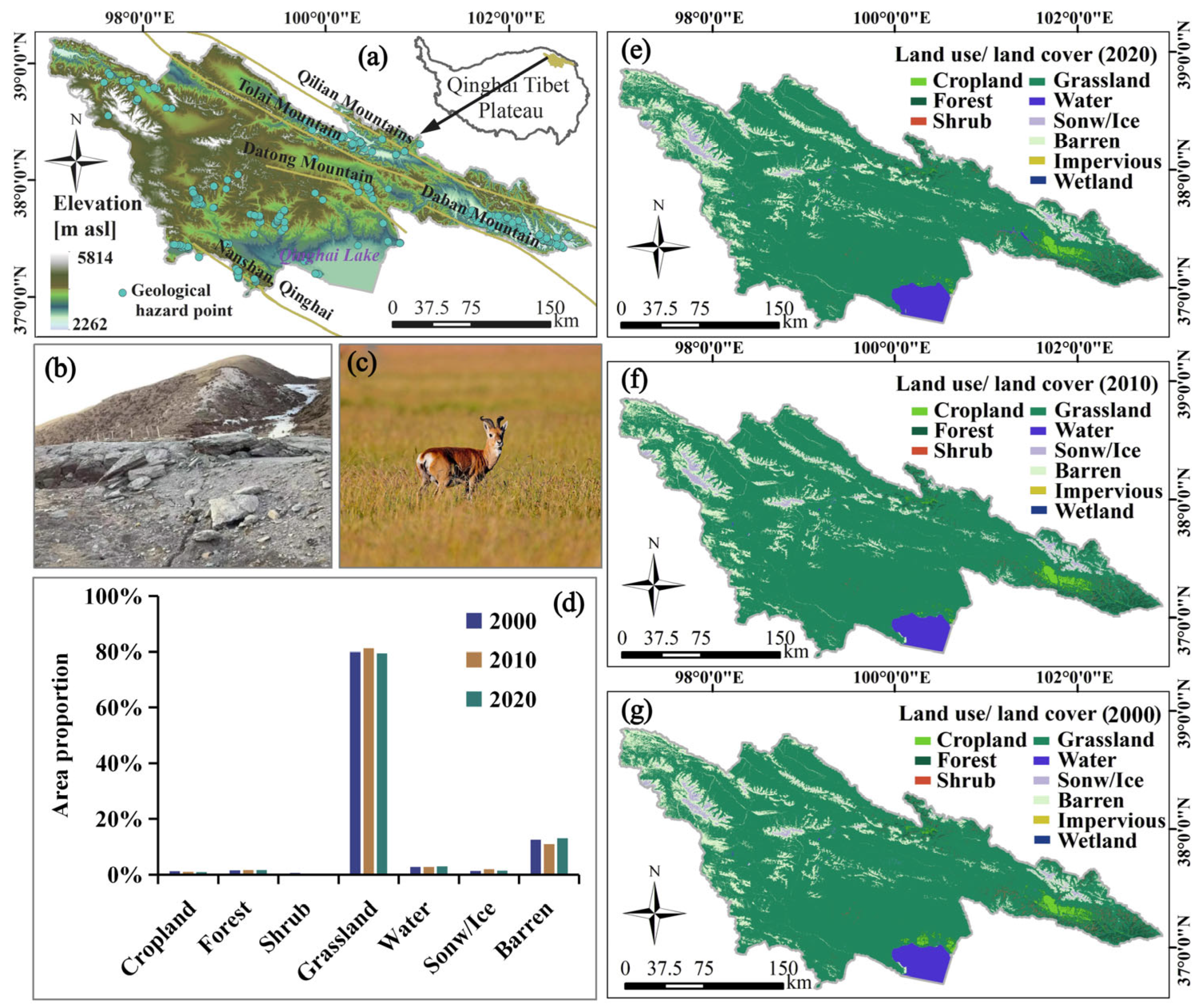
2.1. Study Area

Focusing on northern Qinghai’s Ecological Security Barrier Area (centered on the Qilian Mountain glacier-water conservation zone; Figure 1), this study examines a region of critical ecological significance—hosting Qinghai Lake’s world-class wetlands (key breeding grounds for plateau birds) and the sole global habitat of endangered Przewalski’s gazelle (Procapra przewalskii; Figure 1f) [30]. Simultaneously, it faces severe environmental degradation, including glacier retreat, vegetation loss, and desertification driven by climate change and human activities [31], compounded by frequent geological hazards (e.g., landslides, debris flows; Figure 1e) due to its mountainous, fault-prone terrain [32]. This convergence of high-value ecosystems and multiscale stressors makes it imperative to quantify resilience through landscape structural metrics to capture spatial heterogeneity, integrate disaster risk assessment, and leverage FLUS-based scenario simulations for anticipatory conservation planning. Thus, the area serves as an ideal validation site for our integrated resilience framework, aligning core research innovations with urgent regional ecological security needs.

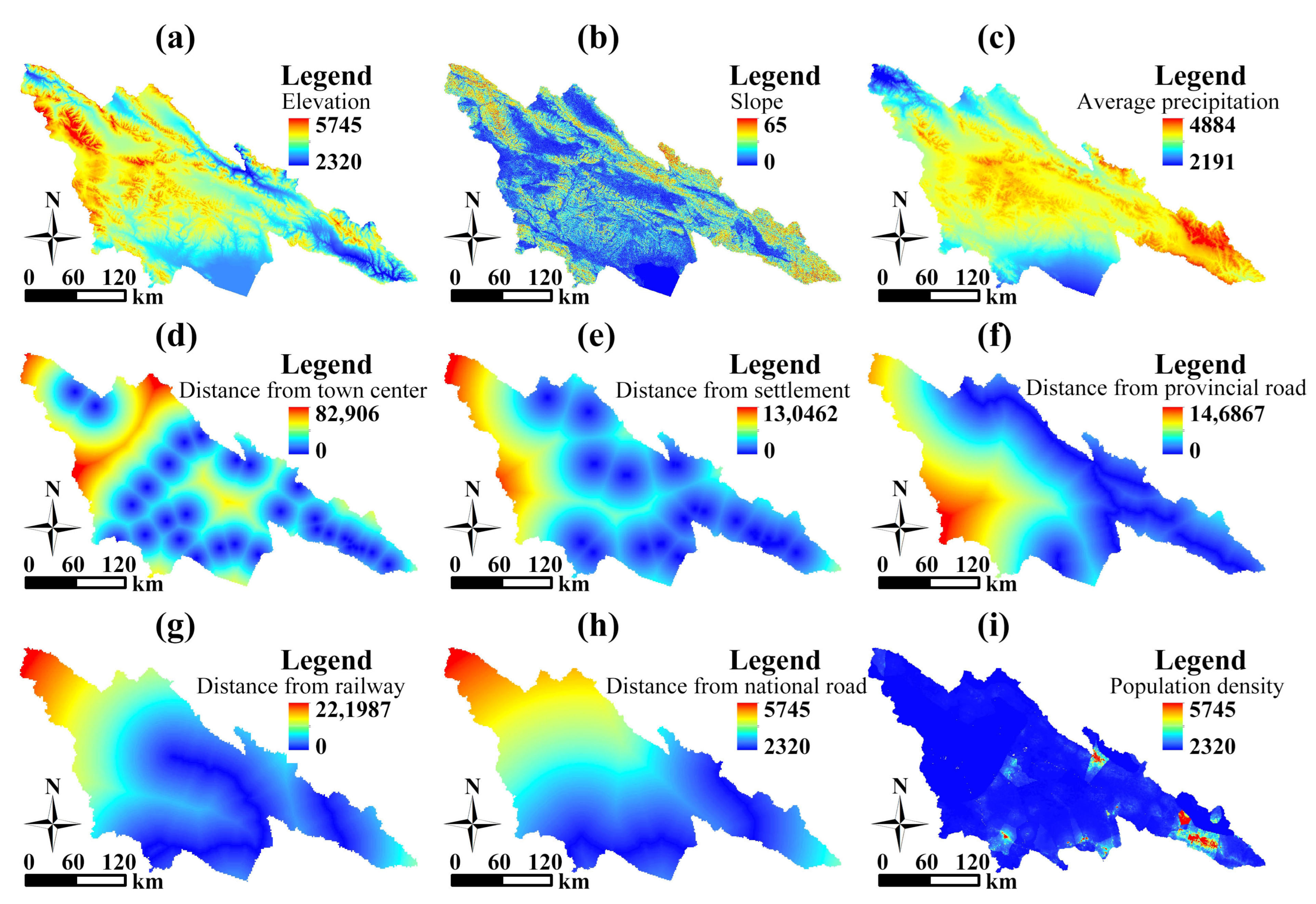
2.2. Data Sources and Data Processing

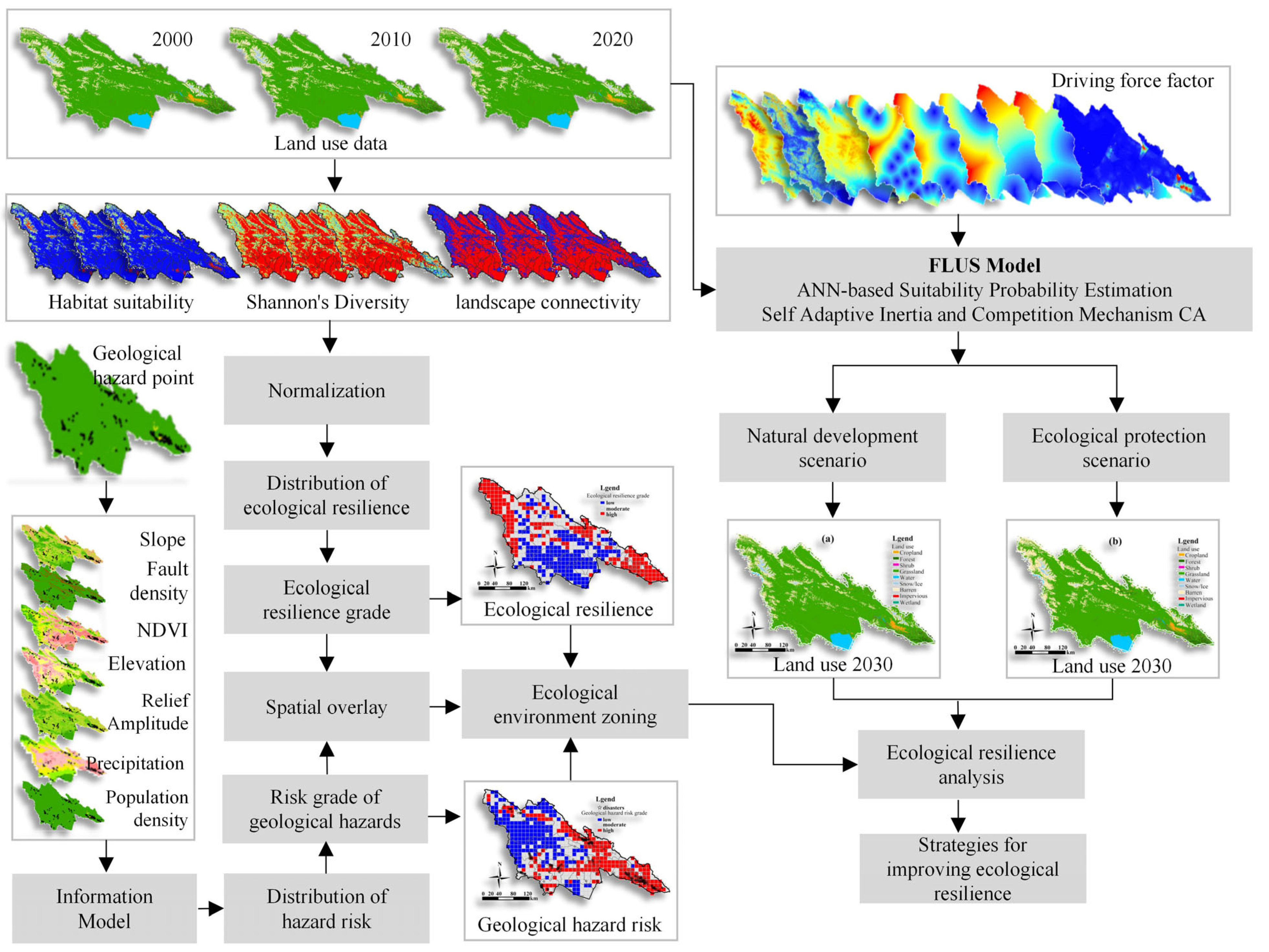
Spatial assessment of ecological resilience using multi-source datasets (

Table 1. Summary of the primary data.

Data Type	Data Format	Data Source/Processing	Spatial Resolution
Land use/land cover	Raster	Wuhan University 1990–2020 China 30 m Land Cover Dataset (http://doi.org/10.5281/zenodo.4417809, accessed on 1 February 2022)	30 m
Digital elevation model (DEM)	Raster	Resource and Environmental Science and Data Center (https://www.resdc.cn, accessed on 1 February 2022)	30 m
Geological disaster data (1960–2020)	Excel	1:100,000 county-level geological disaster survey and the government report	-
Precipitation	Raster	Resource and Environmental Science and Data Center (https://www.resdc.cn, accessed on 1 February 2022)	1 km
NDVI	Raster	Resource and Environmental Science and Data Center (https://www.resdc.cn, accessed on 1 February 2022)	1 km
Population density	Raster	Resource and Environmental Science and Data Center (https://www.resdc.cn, accessed on 1 February 2022)	1 km
Strike slip fault	Vector	National Earth System Science Data Center (http://www.geodata.cn, accessed on 1 February 2022)	-
Railway	Vector	Geospatial data cloud (http://www.gscloud.cn/, accessed on 1 February 2022)	-
Provincial road	Vector	Geospatial data cloud (http://www.gscloud.cn/, accessed on 1 February 2022)	-
National road	Vector	Geospatial data cloud (http://www.gscloud.cn/, accessed on 1 February 2022)	-
Settlement	Raster	Resource and Environmental Science and Data Center (https://www.resdc.cn, accessed on 1 February 2022)	1 km
Administrative boundary	Vector	Geospatial data cloud (http://www.gscloud.cn/, accessed on 1 February 2022)	-
Town center	Vector	Geospatial data cloud (http://www.gscloud.cn/, accessed on 1 February 2022)	-

). Land use/land cover data represent 9 thematic categories: cropland, forest, shrub, grassland, water, snow/ice, barren, impervious, and wetland. All raster data with different spatial resolutions in Table 1 are resampled. In this study, we used spatial data with different resolutions. We use the resampling tool of ArcGIS10.2 to resample all spatial raster data to a spatial resolution of 100 m, and we use the nearest neighbor technique to resample spatial data, which is one of the most widely used techniques [33].

2.3. Methodology

Our research method includes four steps: (1) Explore the change of land use in ecological barrier areas in northern Qinghai in 2000, 2010, and 2020. (2) Study the distribution and change of ecological resilience of ecological barrier areas in northern Qinghai over three time periods. (3) Carry out ecological zoning planning according to the spatial distribution of ecological resilience in 2020 and the results of geological disaster risk assessment. (4) Use the FLUS model, combined with the results of ecological zoning planning, to predict the ecological resilience in inertia development (ID) scenarios and ecological protection (EP) scenarios in 2030. Figure 2 illustrates the schematic diagram of our research method.

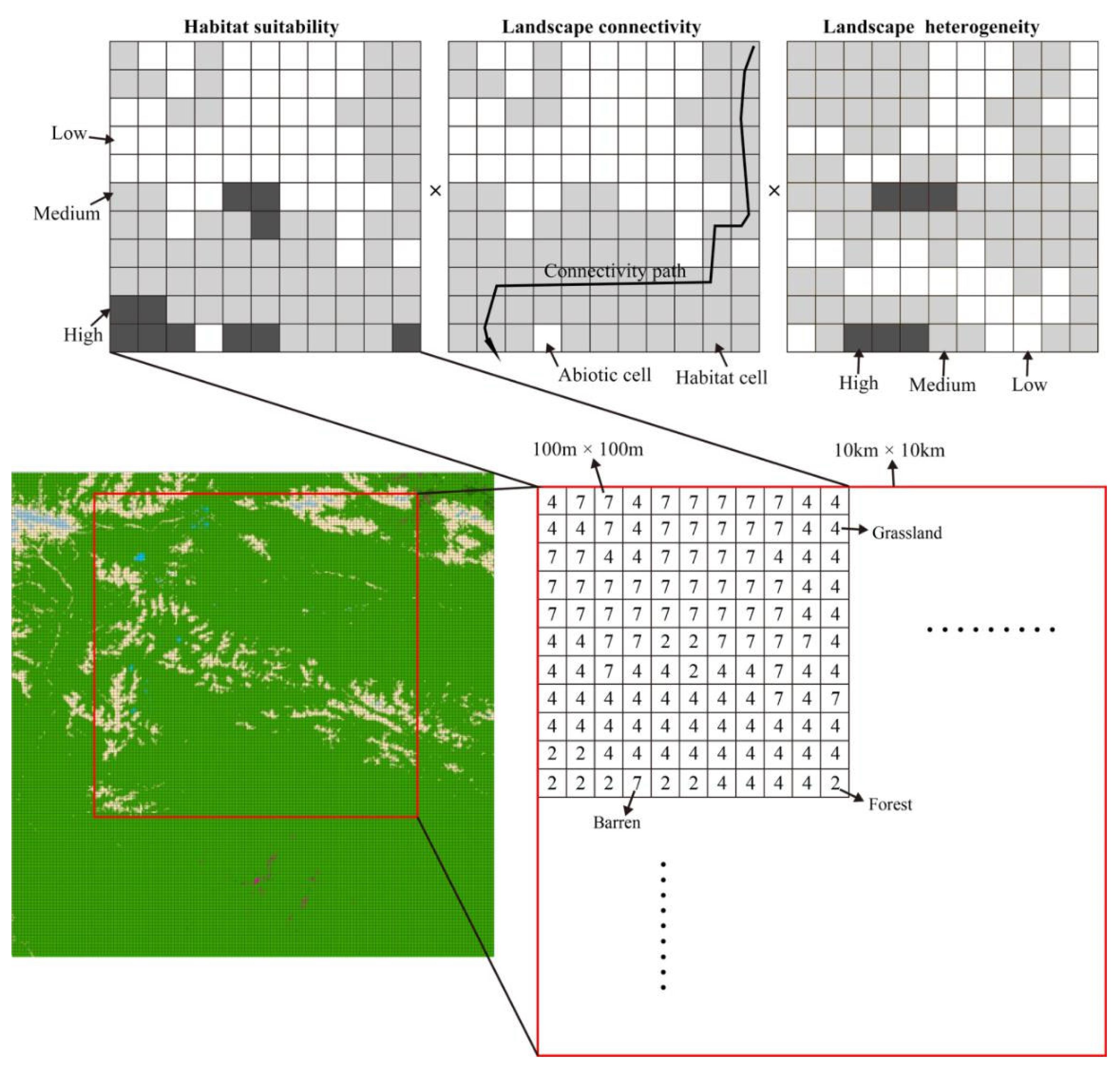
2.3.1. Calculation Method of Ecological Resilience

From the perspective of the risk resistance, adaptability, and resilience of ecosystems, different landscape background elements have different risk resistance levels. For example, compared with land used for construction, which has higher human activity intensity, landscape elements such as woodland, grassland, and water areas have higher natural habitat suitability [34,35,36] and can have higher resistance to ecological risks [37,38]. Landscape heterogeneity can affect the stability and complexity of landscape ecosystems and plays an important role in promoting the energy flow and material circulation of landscape ecosystems and in reducing the spread of ecological disturbance [39,40,41]. It can identify patches that have important contributions to biological diffusion and can be used as a measure of resilience. In this paper, landscape pattern indicators are integrated into the research paradigm of the risk resistance, adaptability, and resilience of ecosystems. Landscape suitability, landscape connectivity, and landscape diversity are selected as the main indicators for ecological resilience calculation (Figure 3). In addition, the calculations of resistance, adaptability, and resilience have different units; therefore, data standardization is needed when using multiple indicators for evaluation. In this study, these three factors are standardized to [0, 1]. The formula is as follows:

$$E{R}_i=H{S}_i\times SHD{I}_i\times LC{I}_i$$

(1)

where $E{R}_i$ represents the ecological toughness of Grid $i$; $H{S}_i$ represents the landscape suitability of Grid $i$; $H{S}_i$ is selected according to the land use type of Grid $i$, with the coefficient shown in

Table 2. Habitat suitability of different land types [34,35,36].

Cropland	Forest	Shrub	Grassland	Water	Snow/Ice	Barren	Impervious	Wetland
0.5	1	1	0.7	1	0.1	0.6	0	1

; $SHD{I}_i$ represents the Shannon Diversity Index of grid B, $LC{I}_i$ is the Landscape Connectivity Index of grid B; and $SHD{I}_i$ and $LC{I}_i$ are calculated by Fragstats software (https://fragstats.org, accessed on 1 February 2022).

2.3.2. ${\mathrm{Getis}-\mathrm{Ord} \mathrm{G}}_{\mathrm{i}}$ Index

The ${\mathrm{Getis}-\mathrm{Ord} \mathrm{G}}_{\mathrm{i}}$ Index mainly reveals the similarity or correlation between the attribute eigenvalues of spatial regional units and their adjacent spatial units by analyzing the information in the area; then, it identifies the spatial distribution of “hot and cold spot areas” and carries out a data heterogeneity test. The calculation formula is as follows:

$$G_i(d)={\displaystyle \frac{{\displaystyle {\sum }_{j=1}^n{w}_{ij}(d)x_j}}{{\displaystyle {\sum }_{j=1}^n{x}_j}}}(i\ne j)$$

$$Z(G_i)={\displaystyle \frac{G_i-E(G_i)}{\sqrt{Var(G_i)}}}$$

where $w_{ij}$ represents the elements of spatial weight matrix $W$, which is 1 when adjacent in space and 0 when not adjacent. $E(G_i)$ and $Var(G_i)$ are the mathematical expectation and variance of $G_i$, respectively. If $Z(G_i)$ is positive and significant, it indicates that the value around position $i$ is relatively high, showing a high-value gathering area (hot spot area) in space, and vice versa, showing a low-value gathering area (cold spot area) in space [42].

2.3.3. Information Quantity Method

The information quantity method transforms the geographical environment information in the study area into the information quantity value reflecting the geological stability, and the information quantity value of the index can measure its contribution rate in the occurrence of geological disasters [43,44,45], so as to evaluate the state of each geographical environment factor and the possibility of geological disasters. The information content calculation formula is:

$$I(x_i)=\ln {\displaystyle \frac{N_i/N}{S_i/S}}$$

where $N_i$ is the grid number of geological hazard points in evaluation factor $x_i$; $N$ is the total number of grids containing geological hazard points in the study area; $S_i$ is the number of grids covering the evaluation factor $x_i$; $S$ is the total number of grids in the study area; and $i$ is the type of evaluation factor.

Add the information of all evaluation factors in each grid unit to get the total information in the grid, which is used to characterize the risk of geological disasters. The formula is as follows:

$$R_{\left(GD\right)}={\displaystyle {\sum }_{i=1}^{n}I\left(x_i\right)}={\displaystyle {\sum }_{i=1}^n\ln \frac{N_i/N}{S_i/S}}$$

where $R_{\left(GD\right)}$ is the hazard degree of geological disasters and $n$ is the number of evaluation factors.

2.3.4. FLUS Space–Time Simulation Model

The FLUS model is a new type of land use simulation model that can predict and reflect the future land use situation in the study area. The advantages of this model lie in introducing social and natural spatial autocorrelation factors through the training module of an artificial neural network (ANN) and in introducing the adaptive inertia competition mechanism into a CA module, which can effectively deal with the uncertainty of the mutual transformation of different land types [46], mainly including the following two modules:

(1) Calculation of suitability probability based on a neural network. The artificial neural network algorithm (ANN) is mainly composed of an input layer, a hidden layer and an output layer, and its expression is:

$$p\left(p,k,t\right)={\displaystyle \sum _j{w}_{j,k}sigmoid(ne{t}_j(ne{t}_j(p,t)))={\displaystyle \sum _j{w}_{j,k}\times \frac{1}{1+e^{-ne{t}_j(p,t)}}}}$$

Among them, $p\left(p,k,t\right)$ is the suitability probability of the $k$ land on grid $p$ and time $t$; $w_{j,k}$ is the weight of the hidden layer and the output layer; and $sigmoid$ is the hidden layer to the output layer.

(2) Adaptive inertia competition mechanism. The FLUS model uses an adaptive inertia mechanism to simulate the competition among different regions, and its core is an adaptive inertia coefficient, whose expression is:

$$\begin{array}{l}\begin{array}{cc}Interi& a_k^t=\end{array}\\ \left\{\begin{array}{cc}Interi\hspace{1em}\hspace{1em} a_k^{t-1},\hfill & if\hspace{1em}\left|D_k^{t-1}\right|\le \left|D_k^{t-2}\right|,\\ Interi\hspace{1em}{a}_k^{t-1}\times {\displaystyle \frac{D_k^{t-2}}{D_k^{t-1}}},\hfill & if\hspace{1em}{D}_k^{t-1}<D_k^{t-2}<0,\\ Interi\hspace{1em}{a}_k^{t-1}\times {\displaystyle \frac{D_k^{t-1}}{D_k^{t-2}}},\hfill & if\hspace{1em}0<D_k^{t-2}<D_k^{t-1},\end{array}\right.\end{array}$$

Among them, $D_k^{t-1}$ and $D_k^{t-2}$ are the differences between the grid quantity and demand quantity of the $k$ land at time $t-1$ and $t-2$, respectively. Based on the above method, the change probability of each grid is calculated, and the local classes are assigned to the grids through CA model iteration. The total probability $T{P}_{P,k}^t$ of grid $p$ being converted into land use type $k$ at $t$ time is expressed as follows:

$$T{P}_{P,k}^t=P_{P,k}\times {\Omega }_{p,k}^t\times Interi\hspace{1em}{a}_k^t\times \left(1-S{C}_{c\to k}\right)$$

Among them, $S{C}_{c\to k}$ is the cost of land type $c$ to $k$; $1-S{C}_{c\to k}$ is the difficulty of conversion; and ${\Omega }_{p,k}^t$ is the neighborhood effect [28].

In this study, based on the land use data of the study area in 2010 and 2020 and considering the principle of data availability, nine driving factors of land use were selected (Figure 4), including altitude, slope, annual average precipitation, distance from central towns, settlements, provincial roads, railways, national roads, and population density. The adaptive inertia competition mechanism is used to simulate the land use in different scenarios in 2030 by using the FLUS model’s suitability probability calculation module based on a neural network to determine the expansion probability of nine land use types.

3. Results

3.1. Landscape Background Analysis

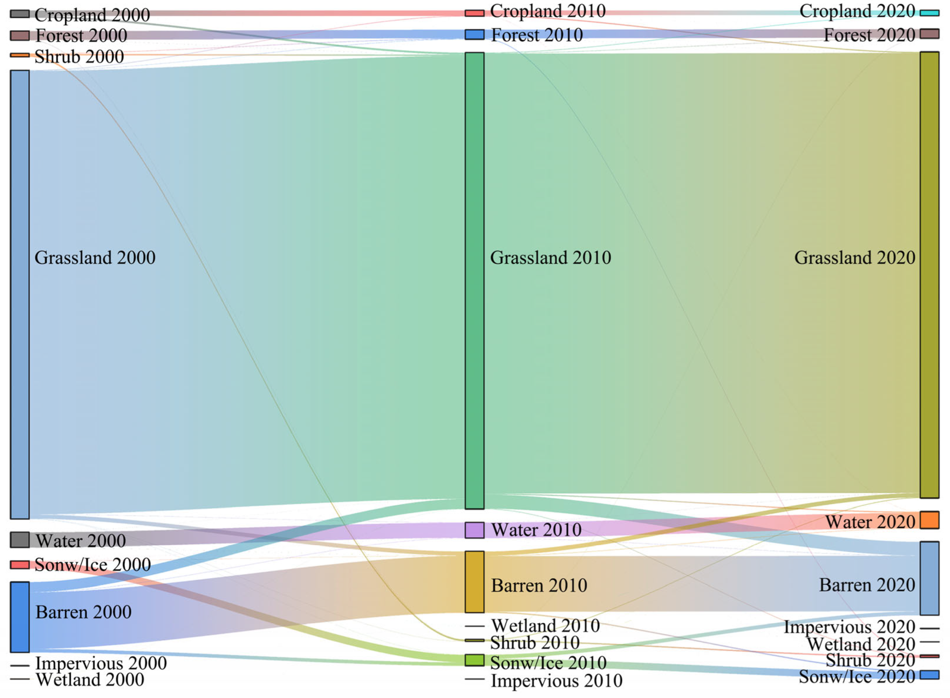
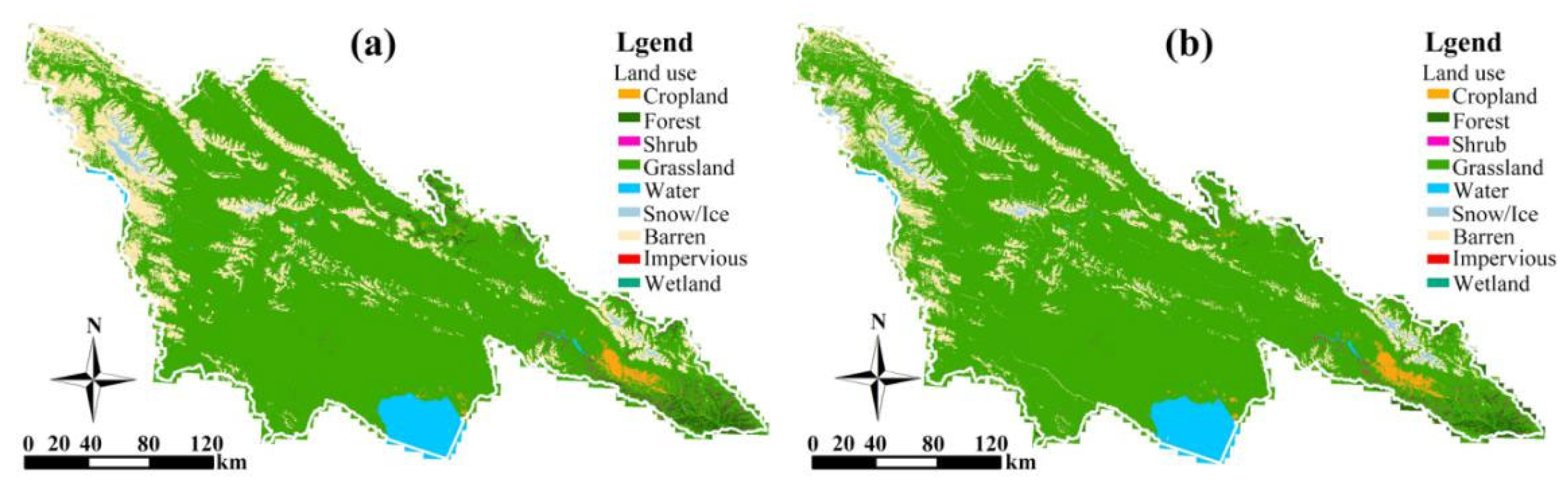
3.1.1. Land Use Change

The land use changes in different periods are illustrated by the transfer matrix (

Table 3. Land use transfer matrix from 2000 to 2020. (Except for the conversion of the same type, the mutual conversion of land types, marked in red, exceeds 100 km²).

2000/2020 (km2)	Cropland	Forest	Shrub	Grassland	Water	Snow/Ice	Barren	Impervious	Wetland
Cropland	478.28	1.25	0	238.34	8.60	0.00	0.44	0.00	0.04
Forest	0.27	809.31	57.00	10.98	0.16	0.00	0.01	0.00	0.00
Shrub	0.00	44.34	141.29	148.71	0.19	0.00	0.01	0.00	0.00
Grassland	56.09	58.06	33.67	42,908.05	107.90	2.97	1191.91	0.00	0.57
Water	0.01	0.04	0.00	4.96	1497.02	1.82	11.57	0.00	0.01
Snow/Ice	0.00	0.00	0.00	0.42	4.64	639.37	123.50	0.00	0.00
Barren	0.59	0.02	0.00	806.07	49.19	189.24	5929.33	0.00	0.00
Impervious	0.00	0.00	0.00	0.00	0.01	0.00	0.00	0.05	0.00
Wetland	0.01	0.00	0.00	8.96	0.17	0.00	0.00	0.00	0.09

) and by the Sangji map (Figure 5). From 2000 to 2020, the areas of forest, water, snow/ice, and barren land increased. Forest area increased by 4.02%; water area increased by 10.06%; snow/ice area increased by 8.53%; and barren area increased by 4.05%. However, the areas of cropland, shrub, grassland, impervious, and wetland all declined. Cropland and shrub areas decreased by 26.37% and 30.67%, respectively, and wetland area decreased by 92.22%. As the main land use type in the study area, grassland area decreased by 0.52% from 2000 to 2020. Grassland was mainly transformed into barren land, and the contradiction between the ecological environment and the grassland degradation caused by social and economic development became more prominent.

According to the differences of land use changes in different periods, it was found that grassland degradation was serious from 2010 to 2020, and the grassland area decreased by 2.21% in this period. The reduced grassland was mainly converted into barren land, with a conversion area of 1192 km². The decrease of shrub area mainly occurred from 2000 to 2010, during which the shrub area decreased by 40.86%. Generally speaking, from 2000 to 2010, the grassland and forest areas increased. From 2010 to 2020, the areas of grassland and forest decreased significantly, and the area of barren land increased significantly; this newly increased barren land mainly came from the transformation of grassland and snow/ice.

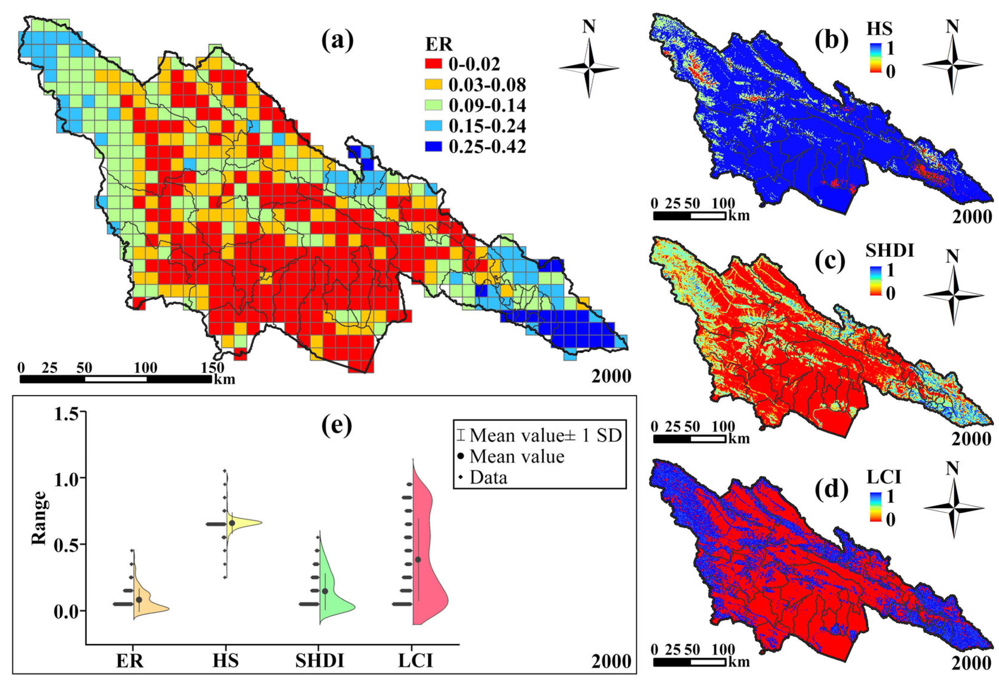
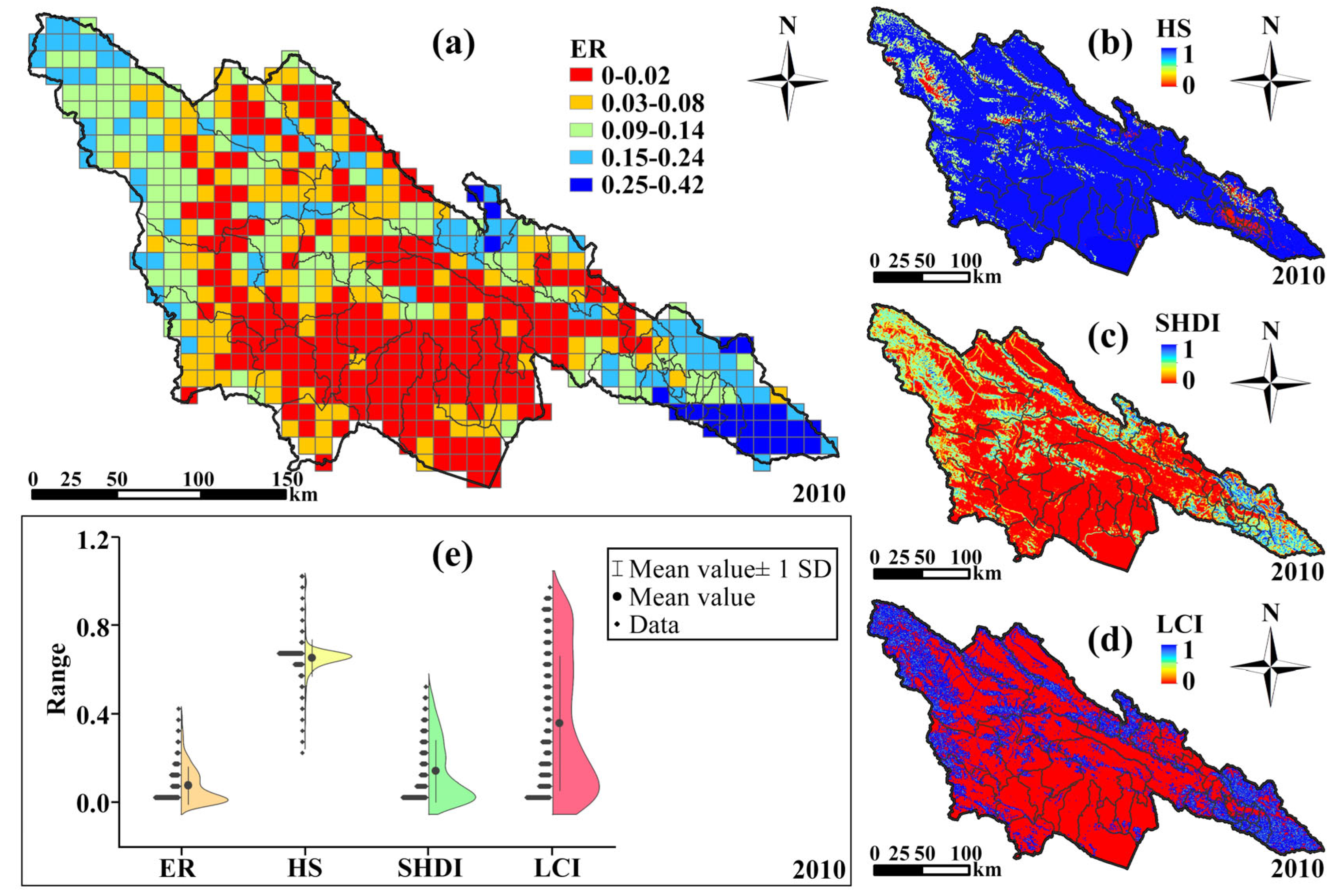
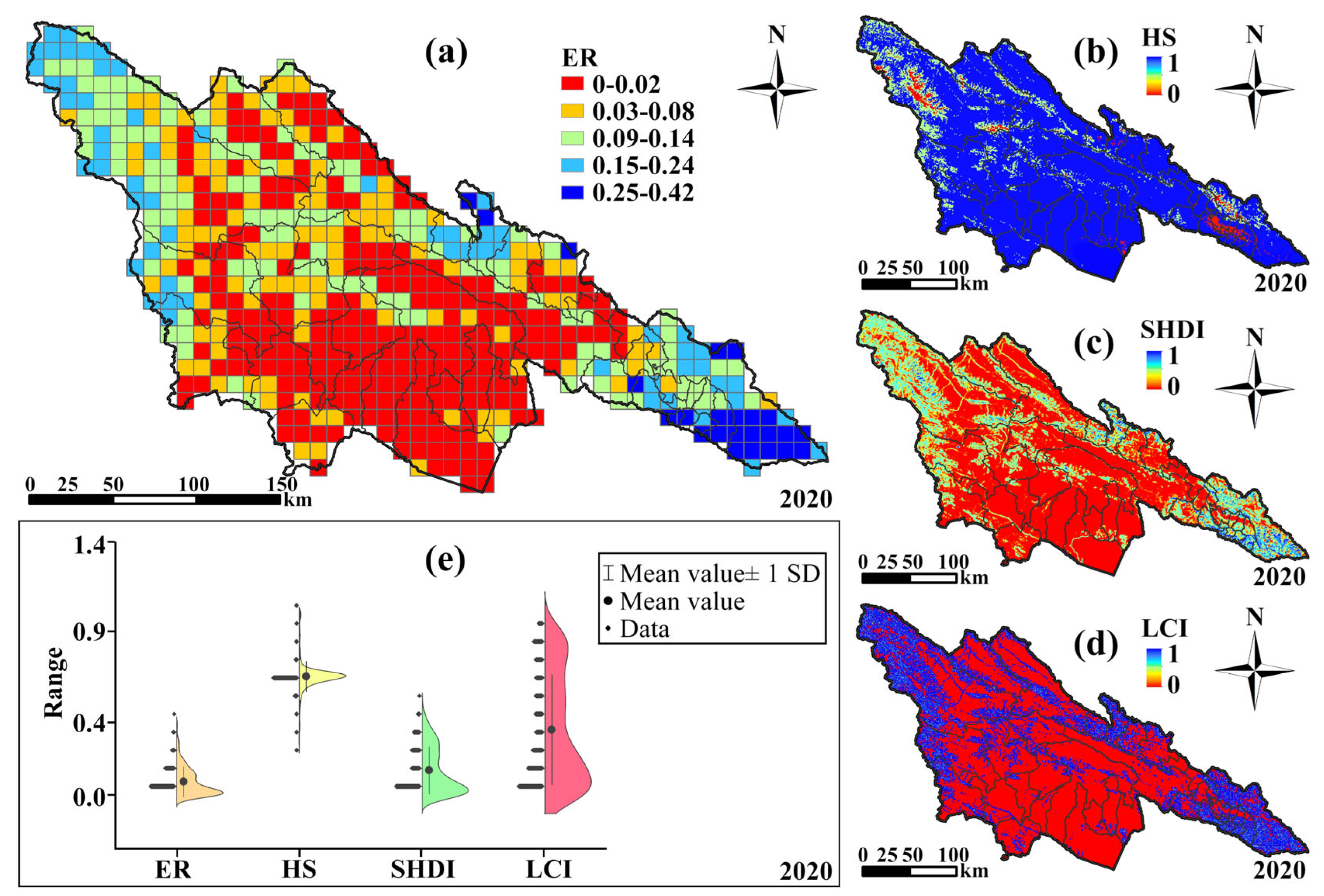
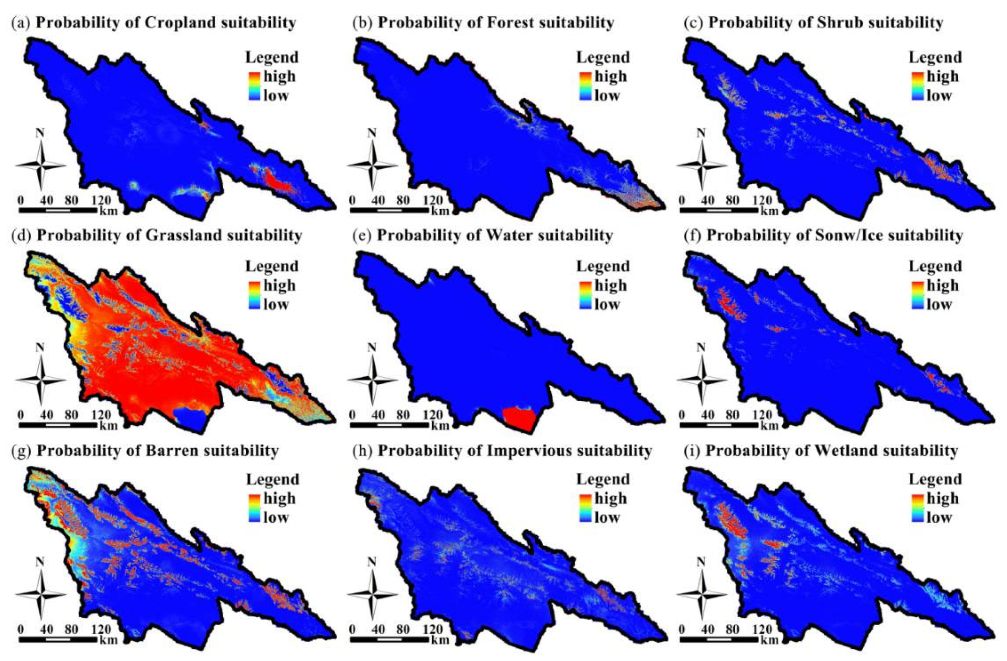
3.1.2. Changes in Landscape Suitability, Connectivity, and Diversity

Table 4. Changes in landscape suitability, connectivity, and diversity from 2000 to 2020 (n = 552, Shapiro–Wilk normality test).

Element		Mean	S.E. Mean	Median	SD	Min	Max	Statistics	p-Value
HS	2000	0.66	0	0.66	0.08	0.25	1.00	0.28	0
	2010	0.66	0	0.66	0.08	0.23	1.00	0.29	0
	2020	0.66	0	0.66	0.08	0.22	1.00	0.30	0
SHDI	2000	0.15	0	0.10	0.14	0	0.57	0.15	0
	2010	0.14	0	0.09	0.14	0	0.53	0.15	0
	2020	0.14	0.01	0.09	0.13	0	0.53	0.15	0
LCI	2000	0.38	0.01	0.31	0.31	0	0.95	0.12	0
	2010	0.36	0.01	0.28	0.30	0	0.95	0.13	0
	2020	0.36	0.01	0.28	0.30	0	0.95	0.13	0

shows the descriptive statistical results of Habitat Suitability (HS), the Landscape Connectivity Index (LCI), and Shannon’s Diversity Index (SHDI) of 552 grids, each with an area of 10 km × 10 km, within the study area. This table also includes the average value of HS, the SHDI, and the LCI as well as the corresponding standard error (Mean ± S.E. Mean), median, standard deviation, minimum value, and maximum value. The Shapiro–Wilk normality test was adopted. The results show that the probability of normal distribution of all elements is 99% (p ≤ 0.01). From 2000 to 2020, there was no significant change in the average value of HS, but the minimum value of HS decreased by 12%. The average values of the SHDI and the LCI decreased. The average value of the SHDI decreased from 0.145 ± 0.006 in 2000 to 0.140 ± 0.006 in 2020, and the average value of LCI decreased from 0.383 ± 0.013 in 2000 to 0.364 ± 0.013 in 2020. On the whole, from 2000 to 2020, we found that there was no obvious change in HS and that the SHDI and the LCI were decreasing all the time. This shows that with the degradation of grassland and with the spread of barren land, the diversity and connectivity of the landscapes in the study area are decreasing.

3.2. Ecological Resilience Assessment Results

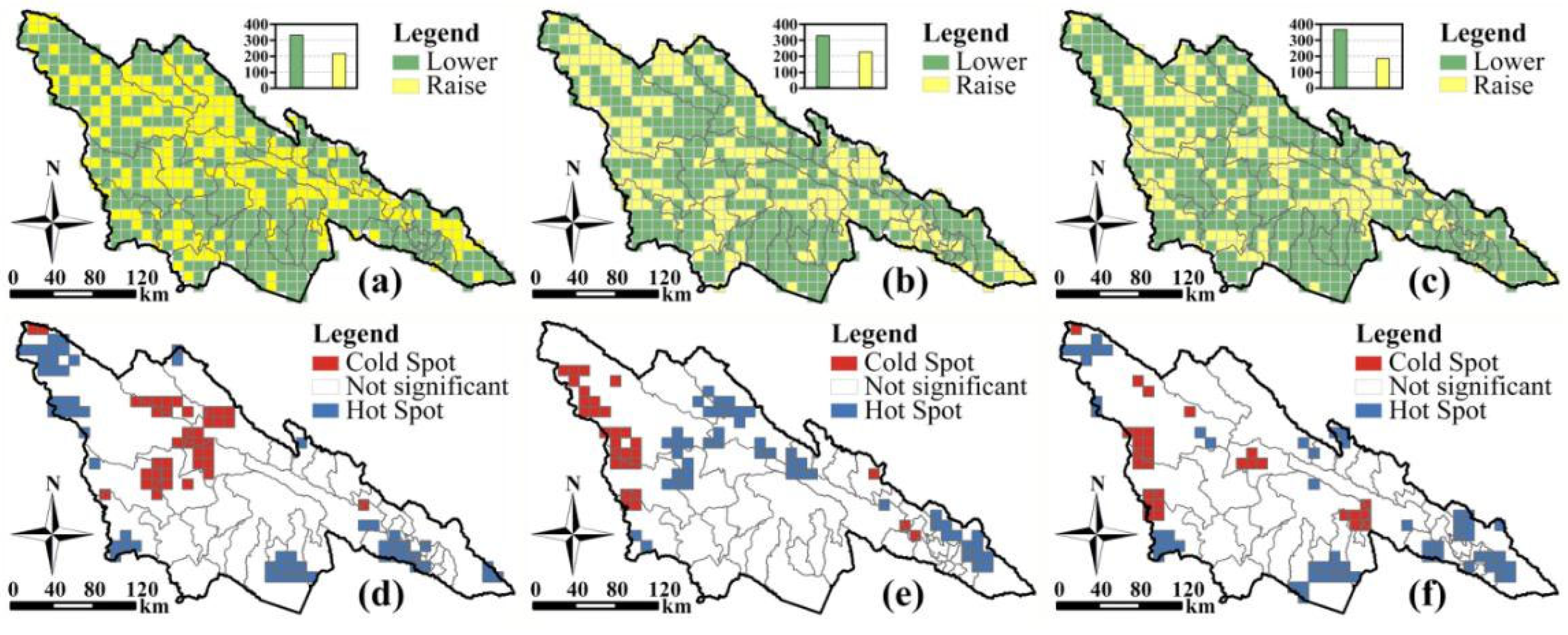
3.2.1. Spatial and Temporal Distribution of Ecological Resilience

We calculated the ER of each year through HS, the SHDI, and the LCI in 2000, 2010, and 2020 (Figure 6, Figure 7 and Figure 8). From the calculation results of ER in different years, the average values of ER in 2000, 2010, and 2020 were 0.082 ± 0.004, 0.079 ± 0.004, and 0.077 ± 0.003, respectively. In 20 years, the average value of ER has decreased by 6%. This signifies progressive destabilization of the ecosystem, manifested through functional attenuation where a diminished Habitat Suitability (HS) and Landscape Connectivity Index (LCI) reflect degraded habitat quality and disrupted energy/material flows. Concurrently, a declining Shannon’s Diversity Index (SHDI) suggests homogenization of landscape patterns, thereby diminishing the system’s adaptive capacity.

Ecological resilience values in 2000, 2010, and 2020 were graded using the natural break point method (Figure 6a, Figure 7a and Figure 8a). From the distribution of different ER intervals, the interval with the highest ER value is mainly distributed in Qilian Mountain National Park in the east of the study area. This is mainly due to the formation of forests in this area, as well as compound ecosystems with wetlands and grasslands. At the same time, development is forbidden or restricted in the main functional areas of this national park; therefore, higher values for HS and on the SHDI and the LCI make the ER value of this region higher. We found that the low ER showed a planar distribution in the central Qinghai Lake basin. Qinghai Lake is a famous scenic spot on the Qinghai–Tibet Plateau. High-intensity tourist pressure during the autumn season has brought many problems to the ecological environment of Qinghai Lake Nature Reserve. At the same time, the land surface cover of the Qinghai Lake Basin area is mainly grassland, and the regional landscape diversity is weak.

3.2.2. Dynamic Change of Ecological Resilience

We calculated the ER value changes of 552 grids in the three periods of 2000–2010, 2010–2020, and 2000–2020. The change values were divided into two categories according to <0 and >0, and the cold and hot spots were analyzed according to the ER change values of each grid (Figure 9). From 2000 to 2010, the ER value of 334 grids decreased, and that of 218 grids increased. By combining the cold spots and the hot spots of ER change that occurred during 2000–2010, we found that the hot spots with higher ER values in this timeframe were mainly concentrated in Yeniugou Township, Yanglong Township, Muli Town, and Longmen Township in the north of the study area. From 2010 to 2020, the ER value of 328 grids decreased, and that of 224 grids increased. The hot spots with higher ER values were mainly concentrated in Suli Township on the western edge of the study area during this period.

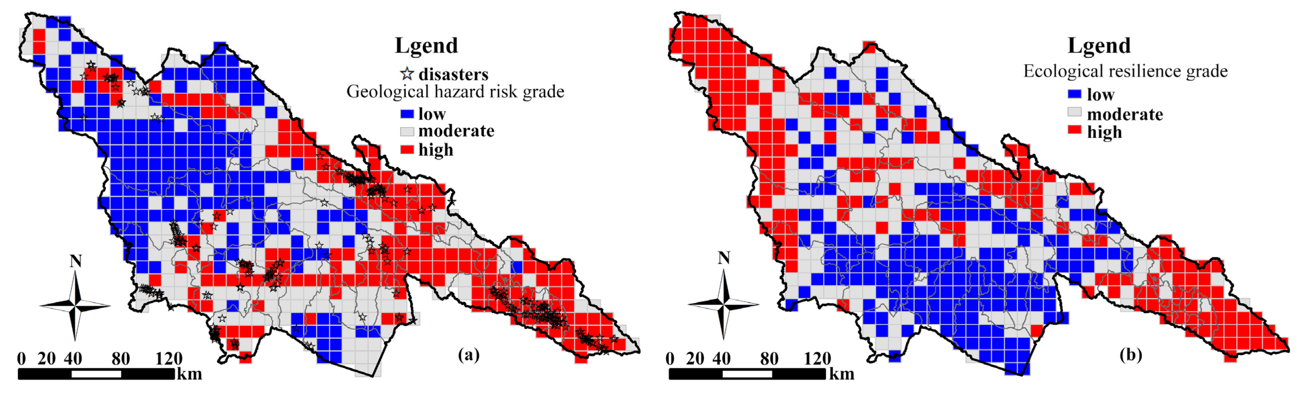
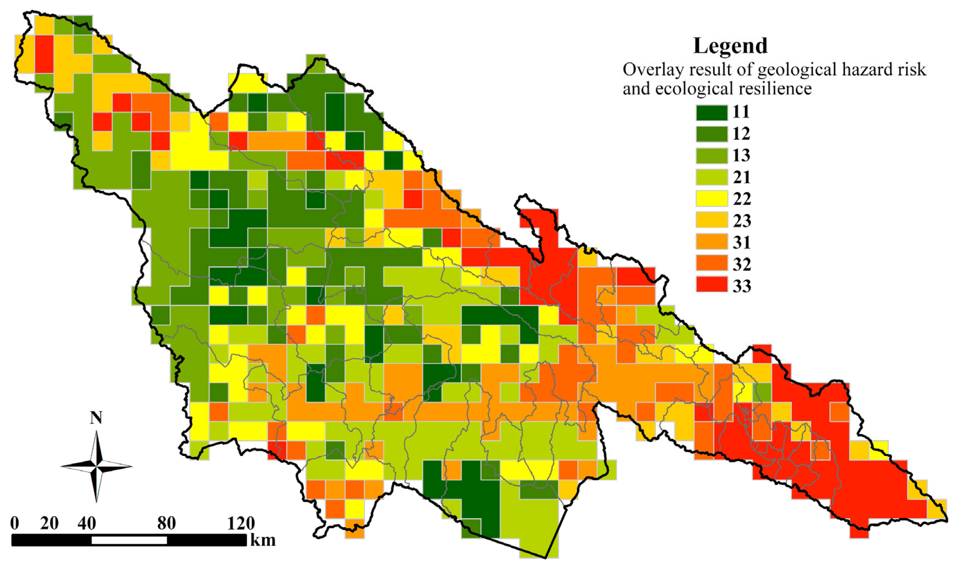
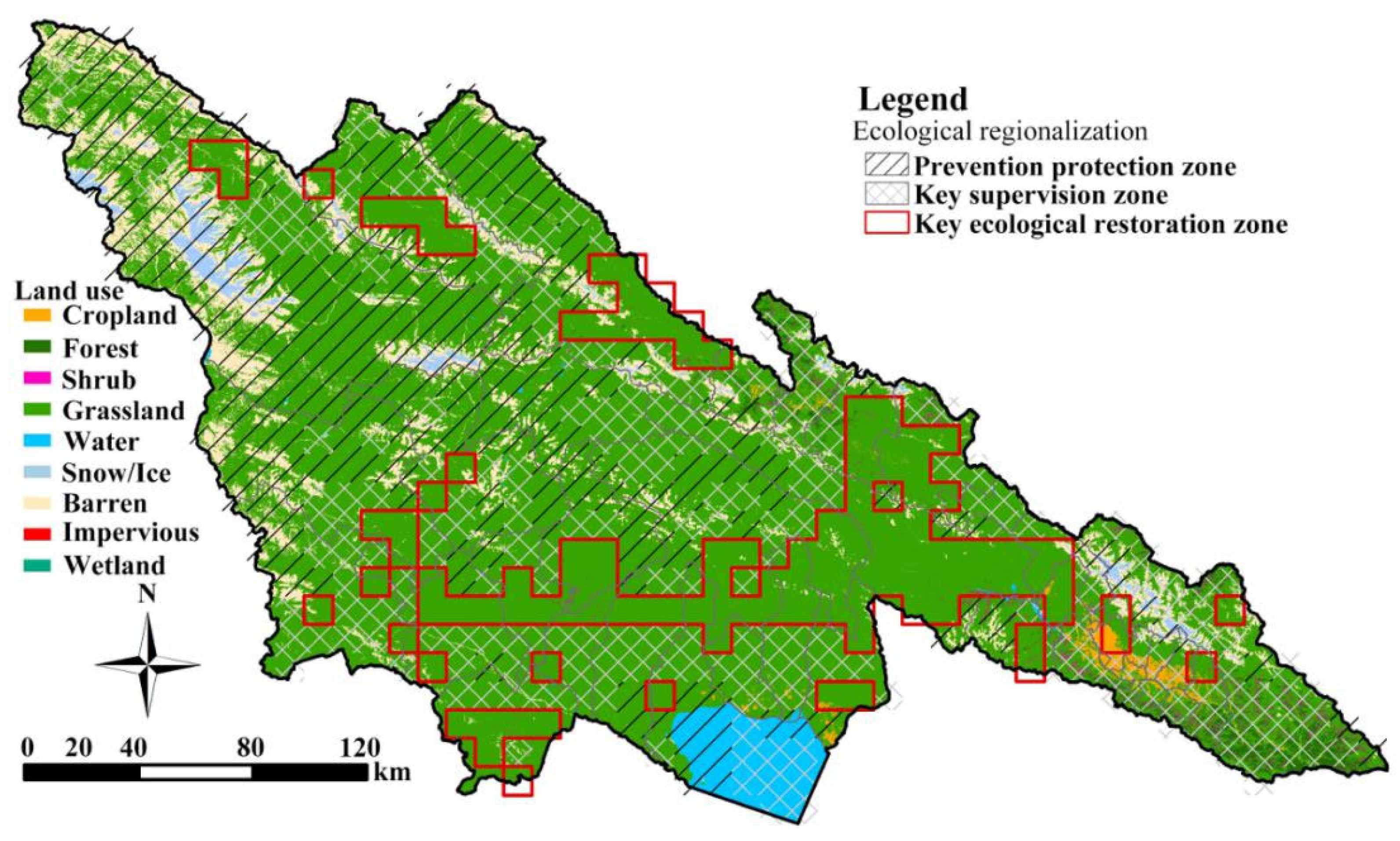
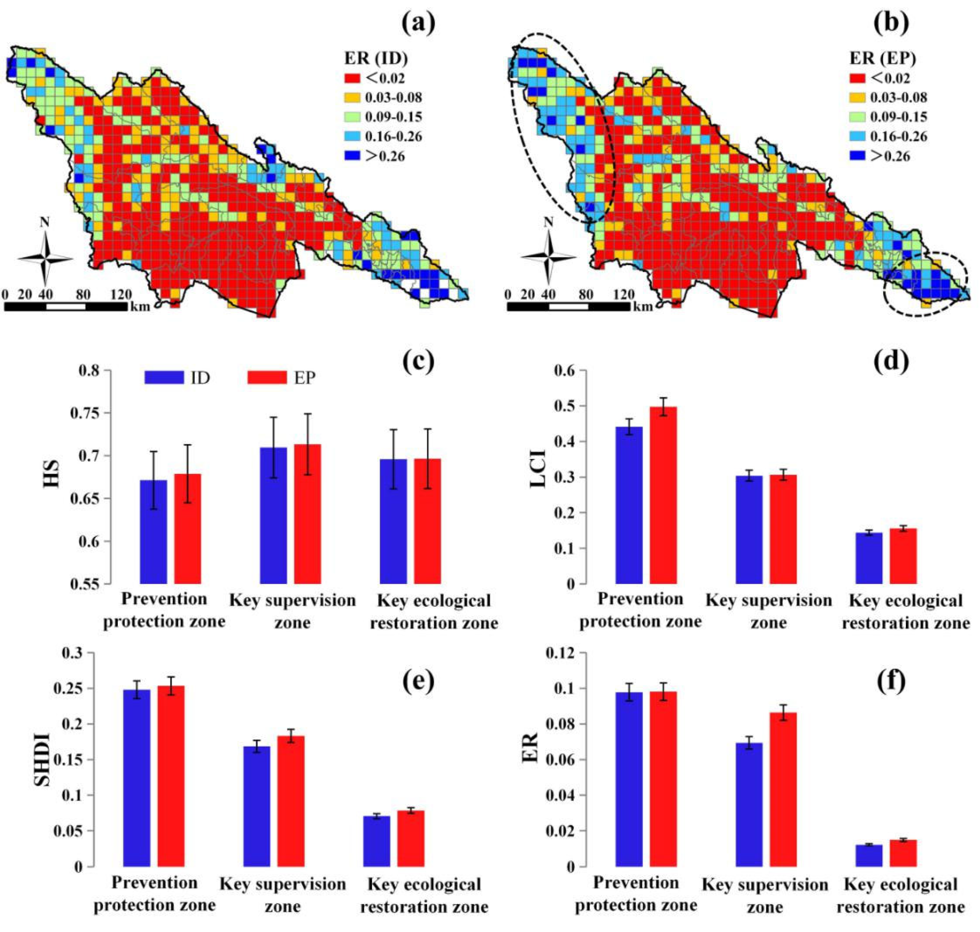
3.3. Ecological Zoning Planning

Frequent geological disasters in the study area have changed the surface cover, destroyed the landscape diversity and connectivity, and thus affected the ecological resilience. In this paper, the results of ecological resilience assessment and geological disaster assessment are further superimposed, so as to put forward the ecological zoning planning under the stress of geological disasters.

Table 5. Information value of geological hazard risk assessment factors [43,44,45].

Category	Evaluation Factor	Grade	Ni	Ni/N	Si	Si/S	Information Value
Geological environment	Slope	<5	3	0.04	51	0.09	−0.96
		5–10	16	0.19	131	0.23	−0.23
		10–15	20	0.24	145	0.26	−0.11
		15–25	36	0.42	178	0.32	0.27
		>25	10	0.12	47	0.09	0.32
	Fault density	<0.04	34	0.40	221	0.40	0
		0.04–0.09	24	0.28	121	0.21	0.25
		0.09–0.16	13	0.15	120	0.22	−0.35
		0.16–0.25	10	0.12	67	0.12	−0.03
		0.25–0.45	4	0.05	23	0.04	0.12
	NDVI	0.02–0.31	4	0.05	73	0.13	−1.03
		0.31–0.47	13	0.15	98	0.18	−0.15
		0.47–0.61	9	0.11	112	0.20	−0.65
		0.61–0.74	22	0.26	145	0.26	−0.02
		0.74–0.90	37	0.44	124	0.23	0.66
	Elevation	2893–3385	29	0.34	71	0.13	0.98
		3385–3722	16	0.19	123	0.22	−0.17
		3722–3994	25	0.29	135	0.25	0.18
		3994–4280	13	0.15	151	0.27	−0.58
		4280–5021	2	0.02	72	0.13	−1.71
	Topographic undulation	<12	8	0.09	96	0.17	−0.61
		12–21	19	0.22	146	0.26	−0.17
		21–30	28	0.33	148	0.27	0.21
		30–42	18	0.21	103	0.19	0.13
		42–64	12	0.14	59	0.11	0.28
Climate	Precipitation	2475–3126	5	0.06	50	0.09	−0.43
		3126–3511	15	0.18	99	0.18	−0.02
		3511–3779	29	0.34	127	0.23	0.39
		3779–4029	24	0.28	211	0.38	−0.30
		4029–4554	12	0.14	65	0.12	0.18
Human activities	≥15° slope road density	<0.023	32	0.38	365	0.66	−0.56
		0.02–0.07	18	0.21	111	0.20	0.05
		0.07–0.14	20	0.24	50	0.09	0.96
		0.14–0.26	8	0.09	18	0.03	1.06
		0.26–0.57	7	0.08	8	0.01	1.74

shows the results of slope, fault density, NDVI, altitude, topographic relief, precipitation, and slope road density above 15 that were calculated by information models in different categories and then used to compare the information value provided by different categories of each evaluation index with the occurrence of geological disasters.

We divided the risk of geological disasters and ecological resilience into three levels: low, medium, and high (Figure 10). As can be seen from Figure 10a, the risk of geological disasters is higher in the eastern part of the study area. This area belongs to the bedrock canyon belt of the main tributaries of the Yellow River and the hilly area of the loess red bed, where there are deep-cut, vertical, and steep-walled valleys, high-rise areas, and unstable terrain on the slopes of the front of hills. At the same time, the loose and strong collapsible loess is widely distributed, and its hydraulic properties are poor. And, because of the narrow area, it is a concentrated distribution area of collapses, landslides, debris flows, and other disasters. Moreover, towns, townships, and villages are densely populated with houses and infrastructure, which is a concentrated area of human activities.

By superimposing the risk of geological disasters and ecological resilience, the results shown in Figure 11 are obtained. Among them, 1, 2, and 3 are low, medium, and high, respectively. Nine results are obtained by superposition, namely, low GHR + low ER, low GHR + medium ER, low GHR + high ER, medium GHR + low ER, medium GHR + medium ER, medium GHR + high ER, high GHR + low ER, high GHR + medium ER, and high GHR + high ER. According to the superposition results, three main ecological divisions are further divided into a prevention protection zone, a key supervision zone, and a key ecological restoration zone (Figure 12). Among them, the prevention protection zone refers to the area with low ecological risk and high ecological resilience, so the area is mainly ecological prevention covering an area of 22,600 km², accounting for 40.94% of the total area of the study area. The key supervision zone refers to the area with moderate ecological risk and ecological resilience, which needs to strengthen the monitoring of the ecological environment in order to avoid the deterioration of the ecological environment caused by disaster risk; this key supervision zone covers an area of 21,400 km², accounting for 38.77% of the total area of the study area. The key ecological restoration zone refers to the area with high risk of geological disasters but low ecological toughness, which is prone to geological disasters, and, because of the low ecological toughness, the ecological environment is easily damaged and difficult to recover; this key ecological restoration zone covers an area of 11,200 km², accounting for 20.09% of the total area of the study area.

3.4. Land Use Simulation

The FLUS model not only simulates the land use scenarios of various land use types under the influence of natural conditions and human activities (Figure 13) but also obtains results that have a high display accuracy and that are similar to the actual land use distribution. Based on the spatial distribution of land use in 2010, this study first simulated the land use situation in 2020. Compared with the actual land use situation in 2010, the Kappa coefficient of the simulation results was 0.812 when 10% of the samples were randomly sampled. Generally, when 0.75 < Kappa ≤ 1, the simulation accuracy of the model is high, and the Kappa coefficient can guarantee high accuracy at different sampling rates. In this study, the FOM coefficient, which can better describe the simulation accuracy than the Kappa coefficient, is also used. The FOM coefficient is 0.257. Theoretically, the larger the FOM parameter value, the better the simulation effect and the higher the accuracy. However, the practical verification shows that the results are mostly within 0.3, and the results of 0.1~0.2 are the most common. All the tests are within a reasonable range, meeting the precision requirements of the model. We used the FLUS model to predict the land use data in 2030 under the inertia development (ID) scenario and ecological protection (EP) scenario based on the land use data in 2020 (Figure 14). In the ID scenario, the original parameters of the model were not adjusted. Under the EP scenario, we limited the degradation of grassland and woodland and the increase of barren land.

3.5. Ecological Resilience Prediction of ID and EP Scenarios

Through the land use in 2030 simulated by the ID and EP scenarios, we further predict the future ecological resilience level. From the calculation results of ecological resilience in different scenarios (Figure 15), the average ecological resilience in the ID scenario is 0.059 ± 0.003, and that in the EP scenario is 0.066 ± 0.004. Compared with the EP scenario, the level of ecological resilience in the ID scenario decreases by 10.61%. However, compared with the ecological resilience in 2020, the predicted ecological resilience in 2030 will decrease in both the ID scenario and the EP scenario, with the ecological resilience in the ID scenario decreasing by 23.38% and the EP scenario decreasing by 14.28%. It can be seen that despite the implementation of certain ecological protection policies, the decline of ecological resilience can only be reduced, and it is difficult to stop the decline of ecological resilience.

According to the results of ecological zoning planning, we further discuss the differences of ecological resilience of different ecological planning zones under the ID scenario and the EP scenario. From the average value of ER, there is a small difference in ecological resilience between the ID scenario and the EP scenario in the prevention protection zone, and a big difference in ecological resilience between the key supervision zone and the key ecological restoration zone. In the key supervision zone, the ecological resilience of the ID scenario is 19.58% lower than that of the EP scenario, and that of the key ecological restoration zone is 17.37% lower than that of the EP scenario. The average value of ER shows that under the ID scenario, the ecological resilience of areas with high risk of geological disasters or low ecological resilience has a significant downward trend, while the EP scenario effectively slows down the downward trend of ecological resilience. This decline is primarily driven by ID-driven land transformation processes, including encroachment into high-resilience ecosystems, unregulated expansion of rain-fed cropland, and the replacement of wetland areas by settlements, fragmenting habitats and reducing landscape connectivity. Conversion of alpine meadows to overgrazed grasslands diminishes root biomass, impairing soil retention capacity and accelerating erosion. The EP scenario counteracts these mechanisms through spatially targeted interventions, such as the establishment of wetland conservation buffers for halting habitat encroachment and the implementation of grazing quotas for preserving meadow integrity. These findings demonstrate that ID disproportionately compromises disaster-prone and ecologically fragile areas, while EP’s geographically optimized measures effectively sustain landscape functionality. The pronounced resilience differentials in supervision/restoration zones (−19.58% and −17.37%) validate the necessity of zoning-adapted conservation strategies.

4. Discussion

4.1. Ecological Resilience Assessment Based on Landscape Background Elements

It is important to carry out the work of ecological resilience assessment for ecological protection and restoration of ecological barrier areas in northern Qinghai in order to curb the trend of ecological degradation [30]. Based on the landscape background elements, this study selected evaluation indexes to evaluate the ecological resilience level of ecological barrier areas under the stress of geological disasters. Compared with previous studies [5,10,11], the ecological resilience assessment work carried out in this paper has two advantages. On the one hand, landscape background factors affect the biochemical cycle process and biological genetic variation process [40], and landscape internal structure indicators can effectively represent biodiversity and ecosystem stability. On the other hand, it is very important to put forward future ecological management strategies based on ecological resilience assessment [7]. This paper puts forward an ecological resilience assessment system based on landscape background elements. In order to adjust and optimize the landscape pattern after the ecological resilience evaluation, we can change the regional energy/material flows or directly act on the ecosystem and then improve the level of regional ecological resilience. For example, we introduced the FLUS model so that the prediction of ecological resilience can be obtained through future land use prediction.

4.2. Policy Suggestions

Our assessment reveals a declining trajectory of ecological resilience in northern Qinghai’s barrier area under persistent grassland degradation, though this trend has been partially mitigated by existing conservation zoning [31]. To counter ongoing pressures, we advocate differentiated management strategies aligned with our ecological zoning. Prevention protection zones (low hazard risk, high resilience) should prioritize preemptive policies such as grassland-use quotas and subsidized rotational grazing, coupled with erosion-control vegetation buffers to maintain ecosystem stability. Key supervision zones (high hazard risk, high resilience) require adaptive governance, including real-time geohazard monitoring networks and post-disaster rapid restoration protocols [32], ensuring timely intervention after events like debris flows. Key ecological restoration zones (high hazard risk, low resilience) demand systemic interventions, such as targeted ecological relocation from high-risk slopes and slope stabilization through terracing with deep-rooted vegetation. This tiered approach transforms zoning theory into actionable policy pathways, directing spatially optimized investments where ecological fragility and disaster threats most critically converge.

4.3. Limitations of This Study

There are some limitations in this study. First, only habitat suitability, landscape connectivity, and landscape diversity are considered in the selection of ecological resilience indicators. In addition, some related landscape pattern indicators such as landscape patch area indicators, density indicators, shape indicators, and edge indicators have not been fully considered. In addition, in the land use forecast, more factors could be considered for human activities and natural environment factors of land use change. Finally, the temporal magnitude of the data used in the scenario simulations in the study needs to be further strengthened in order to increase the confidence of the results.

5. Conclusions

As an important ecological barrier area of the Qinghai–Tibet Plateau, the southern foot of Qilian Mountain is seriously stressed by geological disasters, and the degradation of grassland leads to the gradual deterioration of the ecological environment. From 2000 to 2020, the grassland decreased by 0.52%, mainly converted into barren land. With the degradation of grassland and the spread of barren land, landscape diversity and connectivity are also decreasing. In twenty years, the average value of ER has dropped by 6%. Combined with the results of ecological zoning planning of the southern foot of Qilian Mountain in 2020, the changes of ecological resilience in 2030 under the scenarios of inertia development (ID) and ecological protection (EP) were compared. We found that, compared with 2020, the ecological resilience in 2030 decreased by 23.38% under the inertia development scenario and 14.28% under the ecological protection scenario. Under the inertia development scenario (ID), the ecological resilience of the basic areas with high risk of geological disasters or low ecological resilience has an obvious downward trend, while the ecological protection (EP) scenario effectively slows down the downward trend of ecological resilience.

References

1. Grêt-Regamey, A.; Weibel, B. Global assessment of mountain ecosystem services using earth observation data. Ecosyst. Serv. 2020, 46, 101213. [Google Scholar] [CrossRef]
2. de Moraes, A.R.; Chapin, F.S., III; Seixas, C.S. Assessing environmental initiatives through an ecosystem stewardship lens. Ecol. Soc. 2021, 26, 29. [Google Scholar] [CrossRef]
3. Singh, K.; Byun, C.; Bux, F. Ecological restoration of degraded ecosystems in India: Science and practices. Ecol. Eng. 2022, 182, 106708. [Google Scholar] [CrossRef]
4. Mir, M.; Maleki, S.; Rahdari, V. Ecosystem restoration and degradation monitoring using ecological indices. Int. J. Environ. Sci. Technol. 2022, 12, 08. [Google Scholar] [CrossRef]
5. Chen, Y.; Su, X.; Zhou, Q. Study on the Spatiotemporal Evolution and Influencing Factors of Urban Resilience in the Yellow River Basin. Int. J. Environ. Res. Public Health 2021, 18, 10231. [Google Scholar] [CrossRef]
6. Fang, J.; Xiong, K.; Chi, Y.; Song, S.; He, C.; He, S. Research Advancement in Grassland Ecosystem Vulnerability and Ecological Resilience and Its Inspiration for Improving Grassland Ecosystem Services in the Karst Desertification Control. Plants 2022, 11, 1290. [Google Scholar] [CrossRef]
7. Peterson, G.; Allen, C.; Holling, C. Ecological Resilience, Biodiversity, and Scale. Ecosystems 1998, 1, 6–18. [Google Scholar] [CrossRef]
8. Liu, Z.; Xiu, C.; Song, W. Landscape-Based Assessment of Urban Resilience and Its Evolution: A Case Study of the Central City of Shenyang. Sustainability 2019, 11, 2964. [Google Scholar] [CrossRef]
9. McLeod, E.; Shaver, E.C.; Beger, M.; Koss, J.; Grimsditch, G. Using resilience assessments to inform the management and conservation of coral reef ecosystems. J. Environ. Manag. 2021, 277, 111384. [Google Scholar] [CrossRef]
10. You, X.; Sun, Y.; Liu, J. Evolution and analysis of urban resilience and its influencing factors: A case study of Jiangsu Province. China. Nat. Hazards 2022, 113, 1751–1782. [Google Scholar] [CrossRef]
11. Ruan, J.; Chen, Y.B.; Yang, Z.W. Assessment of temporal and spatial progress of urban resilience in Guangzhou under rainstorm scenarios. Int. J. Disaster Risk Reduct. 2021, 66, 102578. [Google Scholar] [CrossRef]
12. Ruiz Agudelo, C.A.; Mazzeo, N.; Díaz, I.; Barral, M.P.; Piñeiro, G.; Gadino, I.; Roche, I.; Acuña, J.R. Land use planning in the Amazon basin: Challenges from resilience thinking. Ecol. Soc. 2020, 25, 8. [Google Scholar] [CrossRef]
13. Chen, H.; Liu, Y.; Hu, L.; Zhang, Z.; Chen, Y.; Tan, Y.; Han, Y. Constructing a Flood-Adaptive Ecological Security Pattern from the Perspective of Ecological Resilience: A Case Study of the Main Urban Area in Wuhan. Int. J. Environ. Res. Public Health 2023, 20, 385. [Google Scholar] [CrossRef]
14. Armitage, D.; Béné, C.; Charles, A.T.; Johnson, D.; Allison, E.H. The interplay of well-being and resilience in applying a social-ecological perspective. Ecol. Soc. 2012, 17, 15. [Google Scholar] [CrossRef]
15. Duo, L.H.; Li, Y.N.; Zhang, M.; Zhao, Y.X.; Wu, Z.H.; Zhao, D.X. Spatiotemporal Pattern Evolution of Urban Ecosystem Resilience Based on “Resistance-Adaptation-Vitality”: A Case Study of Nanchang City. Front. Earth Sci. 2022, 10, 902444. [Google Scholar] [CrossRef]
16. Wang, B.; Cheng, W. Effects of Land Use/Cover on Regional Habitat Quality under Different Geomorphic Types Based on InVEST Model. Remote Sens. 2022, 14, 1279. [Google Scholar] [CrossRef]
17. Yan, D.D.; Yang, X.; Sun, W.H. How do ecological vulnerability and disaster shocks affect livelihood resilience building of farmers and herdsmen: An empirical study based on CNMASS data. Front. Environ. Sci. 2022, 10, 99857. [Google Scholar]
18. Saini, D.; Singh, O.; Sharma TBhardwaj, P. Geoinformatics and analytic hierarchy process based drought vulnerability assessment over a dryland ecosystem of north-western India. Nat. Hazards 2022, 114, 1427–1454. [Google Scholar] [CrossRef]
19. Liu, S.; Yang, Y. Explanation of terms of grey clustering evaluation models. Grey Syst. Theory Appl. 2017, 7, 129–135. [Google Scholar] [CrossRef]
20. Ban, N.; Liu, X.L.; Zhu, C.Y. Landscape Ecological Construction and Spatial Pattern Optimization Design Based on Genetic Algorithm Optimization Neural Network. Wirel. Commun. Mob. Comput. 2022, 2022, 4976361. [Google Scholar] [CrossRef]
21. Duan, W.; Zhang, H.; Wang, C. Deformation Estimation for Time Series InSAR Using Simulated Annealing Algorithm. Sensors 2019, 19, 115. [Google Scholar] [CrossRef]
22. Gebler, D.; Szoszkiewicz, K.; Pietruczuk, K. Modeling of the river ecological status with macrophytes using artificial neural networks. Limnologica 2017, 65, 46–54. [Google Scholar] [CrossRef]
23. Wang, T.; Li, H.B.; Huang, Y. The complex ecological network’s resilience of the Wuhan metropolitan area. Ecol. Indic. 2021, 130, 108101. [Google Scholar] [CrossRef]
24. Zhou, L.; Hu, F.; Wang, B.; Wei, C.Z.; Sun, D.Q.; Wang, S.H. Relationship between urban landscape structure and land surface temperature: Spatial hierarchy and interaction effects. Sustain. Cities Soc. 2022, 80, 103795. [Google Scholar] [CrossRef]
25. Chi, Y.; Shi, H.H.; Zheng, W.; Wang, E.K. Archipelagic landscape patterns and their ecological effects in multiple scales. Ocean. Coast. Manag. 2018, 152, 120–134. [Google Scholar] [CrossRef]
26. Li, Y.; Zeng, C.; Liu, Z.; Cai, B.; Zhang, Y. Integrating Landscape Pattern into Characterising and Optimising Ecosystem Services for Regional Sustainable Development. Land 2022, 11, 140. [Google Scholar] [CrossRef]
27. Liu, H.; Di, H.; Huang, Y.; Zheng, L.; Zhang, Y.A. Comprehensive Study of the Impact of Large-Scale Landscape Pattern Changes on the Watershed Ecosystem. Water 2021, 13, 1361. [Google Scholar] [CrossRef]
28. Wei, Q.Q.; Abudureheman, M.; Halike, A.; Yao, K.X.; Yao, L.; Tang, H.; Tuheti, B. Temporal and spatial variation analysis of habitat quality on the PLUS-InVEST model for Ebinur Lake Basin, China. Ecol. Indic. 2022, 145, 109632. [Google Scholar] [CrossRef]
29. Ma, B.; Wang, X. What is the future of ecological space in Wuhan Metropolitan Area? A multi-scenario simulation based on Markov-FLUS. Ecol. Indic. 2022, 141, 109124. [Google Scholar] [CrossRef]
30. Han, Z.; Song, W.; Deng, X. Responses of Ecosystem Service to Land Use Change in Qinghai Province. Energies 2016, 9, 303. [Google Scholar] [CrossRef]
31. Liu, J.; Xu, X.; Shao, Q. Grassland degradation in the “Three-River Headwaters” region, Qinghai Province. J. Geogr. Sci. 2008, 18, 259–273. [Google Scholar] [CrossRef]
32. Bai, A.J.; Zhu, K.X.; Guan, Q. Characteristics of Meteorological Geology Disasters and Rainfall in Qinghai Plateau. Plateau Mt. Meteorol. Res. 2021, 41, 119–124. [Google Scholar] [CrossRef]
33. Xiao, Y.; Huang, M.D.; Xie, G.D.; Zhen, L. Evaluating the impacts of land use change on ecosystem service values under multiple scenarios in the Hunshandake region of China. Sci. Total Environ. 2022, 850, 158067. [Google Scholar] [CrossRef]
34. Yang, S.; Zhao, W.; Liu, Y.; Wang, S.; Wang, J.; Zhai, R. Influence of land use change on the ecosystem service trade-offs in the ecological restoration area: Dynamics and scenarios in the Yanhe Watershed, China. Sci. Total Environ. 2018, 644, 556–566. [Google Scholar] [CrossRef]
35. Wang, S.; Cui, Z.; Lin, J.; Xie, J.Y.; Su, K. The coupling relationship between urbanization and ecological resilience in the Pearl River Delta. J. Geogr. Sci. 2022, 32, 44–64. [Google Scholar] [CrossRef]
36. Dai, L.; Li, S.; Le, B.J.; Wu, J.; Yu, D.; Zhou, W.; Zhou, L.; Wu, S. The influence of land use change on the spatial–temporal variability of habitat quality between 1990 and 2010 in northeast china. J. For. Res. 2019, 30, 2227–2236. [Google Scholar] [CrossRef]
37. Tarr, N.M. Demonstrating a conceptual model for multispecies landscape pattern indices in landscape conservation. Landsc. Ecol. 2019, 34, 2133–2147. [Google Scholar] [CrossRef]
38. Liu, P.J.; Hu, Y.C.; Jia, W.T. Land use optimization research based on FLUS model and ecosystem services–setting Jinan City as an example. Urban. Clim. 2021, 40, 100984. [Google Scholar] [CrossRef]
39. Guo, Y.; Liu, Y. Connecting regional landscapes by ecological networks in the Greater Pearl River Delta. Landsc. Ecol. Eng. 2017, 13, 265–278. [Google Scholar] [CrossRef]
40. Banks-Leite, C.; Betts, M.G.; Ewers, R.M.; Orme CD, L.; Pigot, A.L. The macroecology of landscape ecology. Trends Ecol. Evol. 2022, 37, 480–487. [Google Scholar] [CrossRef]
41. Gimona, A.; Messager, P.; Occhi, M. CORINE-based landscape indices weakly correlate with plant species richness in a northern European landscape transect. Landsc. Ecol. 2009, 24, 53–64. [Google Scholar] [CrossRef]
42. Fallah Ghalhari, G.; Dadashi Roudbari, A. An investigation on thermal patterns in Iran based on spatial autocorrelation. Theor. Appl. Clim. 2018, 131, 865–876. [Google Scholar] [CrossRef]
43. Ma, J.; Wang, X.; Yuan, G. Evaluation of geological hazard susceptibility based on the regional division information value method. ISPRS Int. J. Geo-Inf. 2023, 12, 17. [Google Scholar] [CrossRef]
44. Niu, H.; Shao, S.; Gao, J.; Jing, H. Research on GIS-based information value model for landslide geological hazards prediction in soil-rock contact zone in southern Shaanxi. Phys. Chem. Earth Parts A/B/C 2024, 133, 103515. [Google Scholar] [CrossRef]
45. Qiao, J.; Jiang, Y.; Lv, F.; Yuan, D.; Bakhtari, M.F.; Zhang, H.; Atif, R. Study on the susceptibility of geological disasters in loess tableland area of northern Shaanxi based on GIS and information quantity model. All Earth 2025, 37, 1–15. [Google Scholar] [CrossRef]
46. Guo, H.J.; Cai, Y.P.; Yang, Z.F.; Zhu, Z.C.; Ouyang, Y.R. Dynamic simulation of coastal wetlands for Guangdong-Hong Kong-Macao Greater Bay area based on multi-temporal Landsat images and FLUS model. Ecol. Indic. 2021, 125, 107559. [Google Scholar] [CrossRef]
Figure 1. Study area. (a) Location of the study area. (b) A 6.9 magnitude earthquake occurred in Menyuan Hui Autonomous County, Tibetan Autonomous Prefecture of Haibei, Qinghai (37.77° N, 101.26° E). (c) Qinghai Lake is the only habitat for the critically endangered species Procapra przewalskii. (d) Land use change in the study area from 2000 to 2020. (e) Land use in 2020. (f) Land use in 2010. (g) Land use in 2000.
Sustainability 17 05436 g001
Figure 2. Technical process.
Sustainability 17 05436 g002
Figure 3. Landscape pattern index of ecological resilience calculation.
Sustainability 17 05436 g003
Figure 4. Driving factors. (a) Altitude. (b) Slope. (c) Average precipitation. (d) Distance from town center. (e) Distance from settlements. (f) Distance from provincial roads. (g) Distance from the railway. (h) Distance from national roads. (i) Population density.
Sustainability 17 05436 g004
Figure 5. Sangji map of land use transformation from 2000 to 2020.
Sustainability 17 05436 g005
Figure 6. Results of calculations in 2000: (a) ER; (b) HS; (c) SHDI; (d) LCI; and (e) violin diagram of evaluation indicators.
Sustainability 17 05436 g006
Figure 7. Results of calculations in 2010: (a) ER; (b) HS; (c) SHDI; (d) LCI; and (e) violin diagram of evaluation indicators.
Sustainability 17 05436 g007
Figure 8. Results of calculations in 2020: (a) ER; (b) HS; (c) SHDI; (d) LCI; and (e) violin diagram of evaluation indicators.
Sustainability 17 05436 g008
Figure 9. ER changes. (a) ER changes from 2000 to 2010. (b) ER changes from 2010 to 2020. (c) ER changes from 2010 to 2020. (d) Cold and hot spots of ER changes from 2000 to 2010. (e) Cold and hot spots of ER changes from 2010–2020. (f) Cold and hot spots of ER changes from 2010 to 2020. The calculation of cold and hot spots in the figure is based on z-scores and p-values, which are used to determine whether a specific location is a hot or cold spot.
Sustainability 17 05436 g009
Figure 10. Risk of geological disasters and ecological resilience. (a) Geological hazard risk level based on information model. (b) Ecological resilience level in 2020.
Sustainability 17 05436 g010
Figure 11. Superimposed results of geological disaster risk and ecological resilience. 11: low GHR+ low ER; 12: low GHR+ medium ER; 13: low GHR+ high ER; 21: Medium GHR+ low ER; 22: medium GHR+ medium ER; 23: medium GHR+ high ER; 31: high GHR+ low ER; 32: high GHR+ medium ER; 33: high GHR+ high ER.
Sustainability 17 05436 g011
Figure 12. Results of ecological zoning planning.
Sustainability 17 05436 g012
Figure 13. Adaptability probability of land use type based on neural network algorithm.
Sustainability 17 05436 g013
Figure 14. Land use pattern in 2030. (a) Inertial development scenario. (b) Ecological protection scenario.
Sustainability 17 05436 g014
Figure 15. Ecological resilience in ID and EP scenarios. (a) Distribution of ecological resilience in ID scenarios. (b) Distribution of ecological resilience in EP scenarios; (cf) Prediction of ecological resilience indexes of different ecological management zones.
Sustainability 17 05436 g015