Sustainable Supply Chain Strategies for Modular-Integrated Construction Using a Hybrid Multi-Agent–Deep Learning Approach

Abstract

Modular integrated construction (MiC) is a cutting-edge approach to construction that significantly improves efficiency and reduces project timelines by prefabricating entire building modules off-site. Despite the operational benefits of MiC, the carbon footprint of its extensive supply chain remains understudied. This study develops a hybrid approach that combines multi-agent simulation (MAS) with deep learning to provide scenario-based estimations of CO₂ emissions, costs, and schedule performance for MiC supply chain. First, we build an MAS model of the MiC supply chain in AnyLogic, representing suppliers, the prefabrication plant, road transport fleets, and the destination site as autonomous agents. Each agent incorporates activity data and emission factors specific to the process. This enables us to translate each movement, including prefabricated components of construction deliveries, module transfers, and module assembly, into kilograms of CO₂ equivalent. We generate 23,000 scenarios for vehicle allocations using the multi-agent model and estimate three key performance indicators (KPIs): cumulative carbon footprint, logistics cost, and project completion time. Then, we train artificial neural network and statistical regression machine learning algorithms to captures the non-linear interactions between fleet allocation decisions and project outcomes. Once trained, the models are used to determine optimal fleet allocation strategies that minimize the carbon footprint, the completion time, and the total cost. The approach can be readily adapted to different MiC configurations and can be extended to include supply chain, production, and assembly disruptions.

1. Introduction

The construction industry significantly impacts the environment, contributing to $36\%$ of $C{O}_2$ emissions in developed countries and accounting for around $40\%$ of global primary energy consumption [1,2]. These emissions play a central role in accelerating climate change. Although the COVID-19 pandemic temporarily reduced global $C{O}_2$ emissions—from 35 Gt in 2019 to 33.3 Gt in 2020 [3,4]—this drop was short-lived. By 2021, emissions rebounded to 34.9 Gt, driven by resumed activity in sectors like construction, energy, and transport [3,5,6]. In the building sector, operational energy demand and emissions have exceeded prepandemic levels, reaching a record 10 Gt $C{O}_2$ in 2021 [4].

Within this context, MiC has emerged as a promising alternative for improving construction efficiency, reducing timelines, and addressing labor shortages. MiC relies on off-site prefabrication of entire building modules, which are later assembled on-site. While this method offers operational advantages, its environmental footprint, particularly in terms of supply chain logistics and transport emissions, remains underexplored. Traditional Life Cycle Assessment (LCA) methods and studies on construction emissions provide valuable but often static snapshots of environmental impact, lacking the capability to simulate dynamic interactions and temporal variability across supply chain stages. These studies have largely focused on material production (e.g., cement, responsible for approximately 1.48 ± 0.20 Gt $C{O}_2$ in 2017 alone [7]), while a more comprehensive, process-level approach is increasingly necessary to support decision making.

Moreover, to meet international climate goals such as those outlined in the Paris Agreement [5,8], it is crucial to optimize the logistics and planning dimensions of modern construction methods. In this regard, data-driven modeling frameworks such as multi-agent systems are necessary to support these decisions and guide the transition toward low-carbon construction. This study aims to address that gap by proposing a hybrid modeling approach that combines MAS and deep learning. Unlike conventional LCA or static models, the MAS framework allows for dynamic, process-level representation of logistics agents such as transport fleets, suppliers, and assembly sites, and their interactions over time. This capability enables more scenario-based assessments, taking into account temporal variability, geographic distribution, and behavioral rules that drive emissions outcomes. Meanwhile, integrating deep learning enhances optimization by learning non-linear relationships from large-scale simulation data and approximating outcomes under varying configurations.

The motivation for this hybrid approach stems from key research gaps. While several studies have assessed carbon emissions from construction materials or supply chains, few have captured the dynamic logistics coordination processes specific to MiC, nor have they integrated AI-driven optimization within simulation frameworks. Recent work has shown how global supply chain restructuring influences $C{O}_2$ emissions, particularly in emerging economies [9], and others have proposed emission-reduction strategies through supply chain monitoring and fleet optimization [10]. However, these approaches are generally static and not tailored to the unique characteristics of MiC, including modular production, variable fleet configurations, and decentralized sourcing.

In parallel with the structural evolution of MiC, digital technologies have increasingly been applied to enhance resilience and environmental performance in construction supply chains. Notably, machine learning (ML) and deep learning (DL) techniques are being used to support demand forecasting, supplier selection, inventory control, and carbon emission prediction [11,12,13]. These approaches enable improved real-time decision making and scenario testing under uncertainty. Additionally, the adoption of MAS allows for the modeling of decentralized, autonomous logistics agents that interact dynamically and adaptively—a capability well-suited to the modular nature and variability of MiC operations [14,15]. Recent studies also explore reinforcement learning and hybrid agent-based frameworks to address online scheduling and real-time coordination in smart factory and construction contexts [16,17].

This work assesses carbon emissions in MiC supply chains using an integrative multi-agent and deep learning approach (Figure 1). We built an MAS model for the MiC supply chain and parameterized it to a case study using available technical, climate, and geographical data. The model was then used to estimate the carbon footprint associated with different supply chain strategies. These strategies involved allocating varying numbers of transport vehicles across the suppliers and the MiC factory. The results from the multi-agent simulations were used to train an artificial neural network capable of rapidly estimating the carbon footprint, completion time, and total cost for each strategy. The surrogate deep learning model was also employed to determine optimal vehicle allocation configurations for different objectives.

The remainder of this paper is structured as follows. Section 2 presents a comprehensive review of related works on MiC supply chains, sustainability strategies, and digital modeling approaches. Section 3 introduces the proposed hybrid methodology, combining multi-agent simulation with deep learning models. Section 4 describes the case study, including model setup, parameter selection, and simulation results. Finally, Section 5 outlines conclusions and future research directions.

2. Related Works

Recent developments in digital construction emphasize the integration of advanced data-driven techniques, including artificial intelligence, machine learning, and blockchain, into supply chain modeling and optimization. These approaches complement modular construction by addressing its inherent complexity, enabling predictive analytics, and ensuring secure and efficient data exchange across stakeholders. This section reviews how such techniques, particularly in the context of MiC, have been applied to optimize logistics, reduce carbon emissions, and improve resilience.

2.1. MiC Supply-Chain Management

The evolution from traditional site-based practices toward off-site construction (OSC) has progressively reshaped supply-chain requirements, culminating in MiC. MiC incorporates structure, envelopes, mechanical-electrical-plumbing (MEP) systems, and interior finishes into volumetric modules manufactured in controlled environments, thereby transferring an unprecedented share of value-adding activities upstream in the construction supply chain [18,19]. Recent advances also integrate additive manufacturing using robotics to further automate module fabrication and enhance precision and efficiency [20].

Although this vertical shift delivers well-documented benefits, i.e., shorter schedules, reduced on-site labor, superior quality control, and lower environmental externalities, it simultaneously amplifies logistical complexity because large, fully fitted modules must be moved just in time from multiple fabrication centers to geographically dispersed sites under tight dimensional and regulatory constraints [21]. Consequently, MiC success hinges on a resilient construction supply chain (CSC) capable of absorbing frequent disturbances such as traffic delays, fabrication rework, or weather-induced site inaccessibility [22,23].

Research works have, therefore, redirected attention toward CSC resilience and information integration [24]. Empirical and modeling studies confirm that transparent data exchange among upstream suppliers, module manufacturers, transporters, and site managers significantly mitigates schedule risk and cost overruns [22,25]. Building information modeling (BIM) underpins this transparency by providing a single source of geometric and semantic information, from the earliest stages of design right through to the operation of the installation [26]. When coupled with Internet-of-Things (IoT) sensor networks, BIM evolves into a cyber-physical mirror of the supply chain in real time [27], enabling dynamic rescheduling and preventive actions [28,29].

Beyond operational efficiency, MiC is increasingly framed as a lever for sustainability and circular-economy objectives. Design-for-disassembly, high reusability of volumetric units, and closed-loop logistics reduce primary material demand and life-cycle greenhouse-gas emissions relative to conventional methods [30,31]. Optimized transport routing further reduces $C{O}_2$ emissions by minimizing empty runs and matching module dispatch to consolidation opportunities [17]. However, recent reviews highlighted that quantitative evidence on cost–benefit trade-offs and environmental investments remains scarce; many studies adopt qualitative or case-study lenses that limit external validity [32,33]. Rigorous, data-driven assessments are, thus, a priority for both practitioners and policymakers evaluating the MiC process.

A parallel research gap concerns decision-support models that explicitly capture the stochastic nature of MiC logistics. Existing deterministic formulations often fail to accommodate variability in module dimensions, travel times, or demand patterns, leading to brittle schedules when confronted with real-world uncertainty [21]. Stochastic programming and robust-optimization approaches are beginning to address these shortcomings by embedding probability distributions within network design and vehicle-routing problems [25].

In parallel to operational modeling and scheduling, recent research emphasizes the role of financial strategy optimization in complex supply chains. In the retail sector, for example, a data-driven framework has been proposed to enhance financial coordination across suppliers and buyers by integrating real-time operational indicators into credit assessment and capital allocation processes [34]. Although developed for retail, this approach highlights the relevance of financial data elements in improving resilience and sustainability. Such frameworks could be adapted to MiC environments, where capital-intensive modular production and decentralized actors require efficient, transparent, and dynamic financial coordination to manage cost variability and reduce supply risk.

Yet, solution scalability for large-scale projects, and integration with BIM/IoT data streams, is still in its early stages. In parallel, the growing complexity of digital information exchange has led to the exploration of alternative architectures. Beyond traditional BIM–IoT integration, recent advancements advocate for blockchain-based architectures to ensure secure and traceable information flow within modular supply chains. Ref. [35] proposed a hybrid blockchain—the InterPlanetary File System (IPFS) framework with proxy re-encryption—to address privacy and scalability concerns in precast construction. Their solution demonstrated low latency and high efficiency in handling large-scale BIM data, enhancing both trust and traceability among stakeholders

Moreover, recent implementations demonstrate how MAS can enable the creation of autonomous supply chains with predictive and self-adaptive capabilities, enhancing system resilience in response to disruptions such as delays, resource scarcity, or demand fluctuations [14]. MAS frameworks have also been used in smart factory settings to manage scheduling through real-time sensor data, enabling distributed optimization of production and logistics processes [16]. By representing suppliers, fabrication plants of construction modules, transport fleets, and assembly site as autonomous agents, MAS reproduces non-linear interactions and emergent phenomena difficult to capture analytically [36]. As reviewed by [15], MAS frameworks have been extensively applied in construction management at both macro (e.g., urban planning, policy modeling) and micro levels (e.g., logistics, scheduling). Their capacity to replicate decentralized decision making and emergent behaviors makes them particularly suitable for MiC environments where transport delays, fabrication constraints, and site availability interact dynamically [15].

2.2. Sustainability Strategies in Off-Site Construction and Modular Integrated Supply Chains

Off-site construction (OSC), encompassing prefabrication and MiC, is increasingly recognized as a promising and sustainable approach to mitigating the environmental impacts of the building sector [37,38]. Globally, the construction industry is responsible for approximately 39% of greenhouse gas (GHG) emissions, with a significant share linked to the production and use of materials [2,39]. While OSC offers notable advantages, such as improved resource efficiency, reduced construction timelines, and enhanced quality control [40,41,42], it also faces sustainability challenges related to emissions from prefabricated elements, complex logistics, and carbon-intensive supply chains. Additionally, systemic barriers, such as industrial inertia, lack of environmental policy incentives, and insufficient awareness among stakeholders, undermine the widespread adoption of MiC despite its environmental potential [40]. Addressing these challenges requires the implementation of comprehensive strategies that enhance the environmental performance of OSC across the entire life cycle.

Strategies to reduce $C{O}_2$ emissions in OSC focus primarily on material innovation, logistics optimization, and eco-design. The adoption of low-carbon materials such as cross-laminated timber (CLT), ground granulated blast furnace slag (GGBS), and recycled steel has shown considerable potential in reducing embodied carbon [43]. For example, substituting Portland cement with GGBS in the construction of the Shard Tower in London led to a reduction of approximately 700 tonnes of $C{O}_2$. Furthermore, the high precision of factory-based manufacturing processes in OSC contributes to a 30–50% reduction in material waste compared to conventional methods, due to better cutting efficiency, reduced on-site damage, and optimized storage and handling. These benefits, when coupled with lifecycle planning and performance-based specifications, significantly improve the sustainability of off-site construction. However, according to [40], the full realization of these benefits requires the removal of knowledge-related and process-related barriers through targeted training programs, stakeholder engagement, and integrated project delivery frameworks.

Transport logistics is another critical domain for reducing emissions in OSC. The implementation of Just-in-Time (JIT) delivery systems and the use of alternative transport modes, such as barges and rail, can significantly lower the carbon footprint associated with material delivery. Nevertheless, volumetric modules used in MiC are often heavy and oversized, complicating logistics. In this regard, the Kai Tak Community Isolation Facility (CIF) in Hong Kong serves as a landmark example [44]: completed in only four months using a fully modular steel structure, the project achieved a 20.7% reduction in embodied carbon compared to a conventional reinforced concrete counterpart. This outcome was primarily due to optimized material use, reduced on-site energy consumption, and minimized waste generation throughout the construction process. Yet, as highlighted by [40], logistics-related barriers, especially in dense urban contexts, can interact with regulatory, technical, and aesthetic concerns, limiting the replicability of such high-performance projects without systemic coordination.

Digital technologies such as BIM and the IoT play a vital role in improving the environmental performance of OSC. BIM enables early-stage simulations of $C{O}_2$ emissions and facilitates optimized eco-design, while IoT sensors support real-time monitoring of energy use, predictive maintenance [45], and end-of-life planning. For instance, the Nightingale Hospital in London [46,47], built using modular methods, recorded a 40% reduction in on-site emissions by leveraging standardized components and digital coordination. Similarly, in the Kai Tak CIF project [44], the integration of BIM and IoT enhanced project tracking, resource efficiency, and waste control, reinforcing the project’s sustainability objectives.

The potential of MiC to contribute to circular construction practices is also gaining attention. Modular components can be designed for disassembly, reuse, and recycling, extending their service life while reducing environmental impacts. The ETASS system developed in Chile, for example, employs a reusable auxiliary structure to stabilize modules during lifting and transport, resulting in a 54.44% reduction in transport-related $C{O}_2$ emissions [48]. Moreover, recent MiC projects in Asia have successfully incorporated digital twins and sensor networks to enhance energy performance monitoring, materials traceability, lifecycle assessment, as well as carbon emission assessment and tracking in prefabricated building materialization [44,49,50]. Despite these advances, urban logistics remains a significant barrier to low-carbon implementation [40]. Urban logistics remains a major barrier to low-carbon transitions, particularly in dense cities where traffic congestion significantly increases pollutant emissions. For example, real-world studies in Madrid show that $C{O}_2$ emissions from urban buses can rise by up to 50%, and NO_x by 85% under severe congestion scenarios [51]. Similarly, the OECD highlights that road traffic is a dominant source of urban air pollution, exacerbated by inefficient traffic flow and urban density [52].

As mentioned in [40], urban and systemic challenges require coordinated strategies that combine technological innovation with enabling policies, incentives, and industrial transformation. To mitigate this, several pilot projects are now deploying electric vehicles for last-mile delivery and using barges for primary transport, thereby reducing emissions and improving logistical efficiency [53].

2.3. Applications of Computer Simulations and Machine Learning for Carbon Footprint Evaluation in MiC

Simulation and machine learning models address carbon footprint evaluation across both general construction and MiC projects. The literature describes simulation frameworks that integrate tools such as 4D BIM with LCA [54] or combine economic input–output LCA with mixed integer linear programming for supply chain emissions [55]. In MiC contexts, studies deploy multi-method simulation approaches—one combining agent-based and discrete-event simulation for logistics planning [56], another integrating multi-agent simulation with design of experiments and metamodeling for multi-modal logistics [17], and a cyber-physical Internet framework paired with a carbon-aware routing protocol [57].

Machine learning methods forecast carbon emissions at various construction stages. In early design, convolutional neural networks optimize carbon performance of architectural designs [58]. At later stages, one study reports embodied carbon estimation using artificial neural networks, support vector regression, and gradient boosting with R² values exceeding 0.7 and an average prediction error of 5.33% [12], while another achieves high precision in building foundations using XGBoost (R² = 0.88, RMSE = 206.62) [13]. A deep neural network also supports forecasting $C{O}_2$ emissions and energy consumption in intelligent construction [59].

Overall, simulation and machine learning techniques rely on diverse data sources and integration methods, ranging from BIM and LCA to agent-based modeling and ensemble learning, to quantify carbon footprints in both general and MiC environments. However, their effectiveness is strongly dependent on the quality, traceability, and security of underlying data infrastructures.

Although simulation and machine learning offer predictive insights, secure and scalable data environments—such as blockchain–IPFS—are essential to ensure integrity and traceability of the data these models rely on. As highlighted by [35], integrating such architectures enables real-time secure access to logistics and production data, thereby improving the operational resilience of MiC supply chains [35].

Recent systematic reviews also highlight the growing interest in applying machine learning techniques not only for predictive emissions modeling but also for classifying and understanding broader Modern Methods of Construction (MMC) ecosystems. In addition to emissions optimization, machine learning has been used to address strategic financial decisions within construction supply chains. For example, data-driven frameworks have been developed to optimize carbon responsibility allocation under emissions trading policies, showing how carbon cost sensitivity affects pricing and emissions outcomes between suppliers and building owners [60]. These economic–ecological models are essential for supporting sustainable procurement and policy compliance in modular supply systems. For instance, ref. [61] applied a hybrid NLP and SLR method to analyze over 600 publications, revealing the underutilization of ML in supply chain optimization despite its potential to enhance MMC traceability, risk prediction, and lifecycle performance mapping [61].

Table 1. A summary of literature studies on carbon footprint estimation and optimization in construction logistics.

Study	Study Type	Application Domain	Estimation Scope	Key Technologies Used
[54]	Simulation	Project-level	Carbon footprint benchmarking and monitoring	4D Building Information Modeling (BIM), Life Cycle Assessment (LCA) tools
[56]	Simulation	MiC supply chain	Logistics planning, project key performance indicators (KPIs): Project duration, MiC-SC costs, emissions	Agent-based modeling, Discrete-event simulation, Taguchi approach
[17]	Hybrid	Multi-modal logistics in MiC	Multi-modal logistics optimization: Project duration, total costs, emissions	Hybrid multi-agent simulation, Design of experiments, Metamodeling
[55]	Simulation	Building supply chain	Supply chain carbon footprint: GHG emissions, economic output	Economic Input-Output Life Cycle Assessment (EIO-LCA), Mixed Integer Linear Programming (MILP)
[57]	Simulation	Modular construction logistics	Routing optimization for carbon emissions reduction	Cyber-Physical Internet framework, Carbon-aware routing protocol
[62]	Review	General Construction	Global and regional supply chain analysis	Input-output analysis, Life cycle assessment
[58]	Machine Learning	Early architectural design stage	Early-stage carbon footprint estimation	Machine Learning Models, Convolutional Neural Networks
[12]	Machine Learning	Design stage, 70 projects in Yangtze River Delta	Embodied carbon emissions prediction	Artificial Neural Network, Support Vector Regression, Extreme Gradient Boosting
[13]	Machine Learning	Building foundations, 35 public buildings in China	Carbon emissions prediction	BIM, Decision Tree, Random Forest, XGBoost, Neural Network
[59]	Machine Learning	Intelligent Construction	CO emissions and energy consumption forecasting	Deep Neural Networks

presents a synthesis of recent studies on carbon footprint estimation and optimization within construction logistics. It summarizes the application domains, estimation scopes, and key technologies used across various simulation and machine learning approaches.

2.4. Assessment Methods for Carbon Emissions and Cost Across the Life Cycle of Buildings

The assessment of carbon emissions and lifecycle costs in construction has traditionally relied on Life Cycle Assessment (LCA), which remains the most prevalent methodology for quantifying environmental impact across different construction phases. In modular and prefabricated contexts, LCA is often integrated with digital tools and optimization algorithms to enhance its accuracy and scope [57,63,64,65]. For example, LCA has been integrated with carbon-optimized routing algorithms—such as those based on the A-star search method—to improve emissions efficiency in modular construction logistics, in ref. [57], and with energy simulation to project decarbonization trajectories for modular solutions [63].

These methods typically assess emissions from cradle to grave, including material extraction, transport, on-site assembly, operation, and, when available, end-of-life scenarios. Other approaches refine traditional LCA by incorporating site-level data, embodied emissions at each supply chain stage, and value-added analysis to improve accuracy [66]. Broader economic frameworks such as environmentally extended input–output (EEIO) models or multi-regional input–output (MRIO) techniques also support benchmarking emissions across entire supply chains [55,67].

However, these methodologies often lack the dynamic and adaptive capabilities required for MiC modeling, where transport logistics, off-site production, and urban delivery constraints are highly variable. Most existing models do not simulate the behavioral and operational dynamics of transport fleets, coordination delays, or site availability that strongly affect both cost and carbon outcomes in MiC environments.

To address these limitations, recent developments have turned to digital twin and cyber-physical frameworks to integrate real-time monitoring with carbon tracking [57,68]. Agent-based and simulation-driven approaches are also increasingly explored to capture time-dependent emissions and economic trade-offs in modular supply chains. While the present study does not apply conventional LCA, it contributes to this growing body of research by proposing a hybrid method that combines multi-agent simulation and deep learning. This allows for scenario-based evaluation of emissions and costs under varying logistics strategies, enabling planners to account for temporal interactions, geographic distribution, and decentralized decision making in a way that complements and extends traditional LCA frameworks.

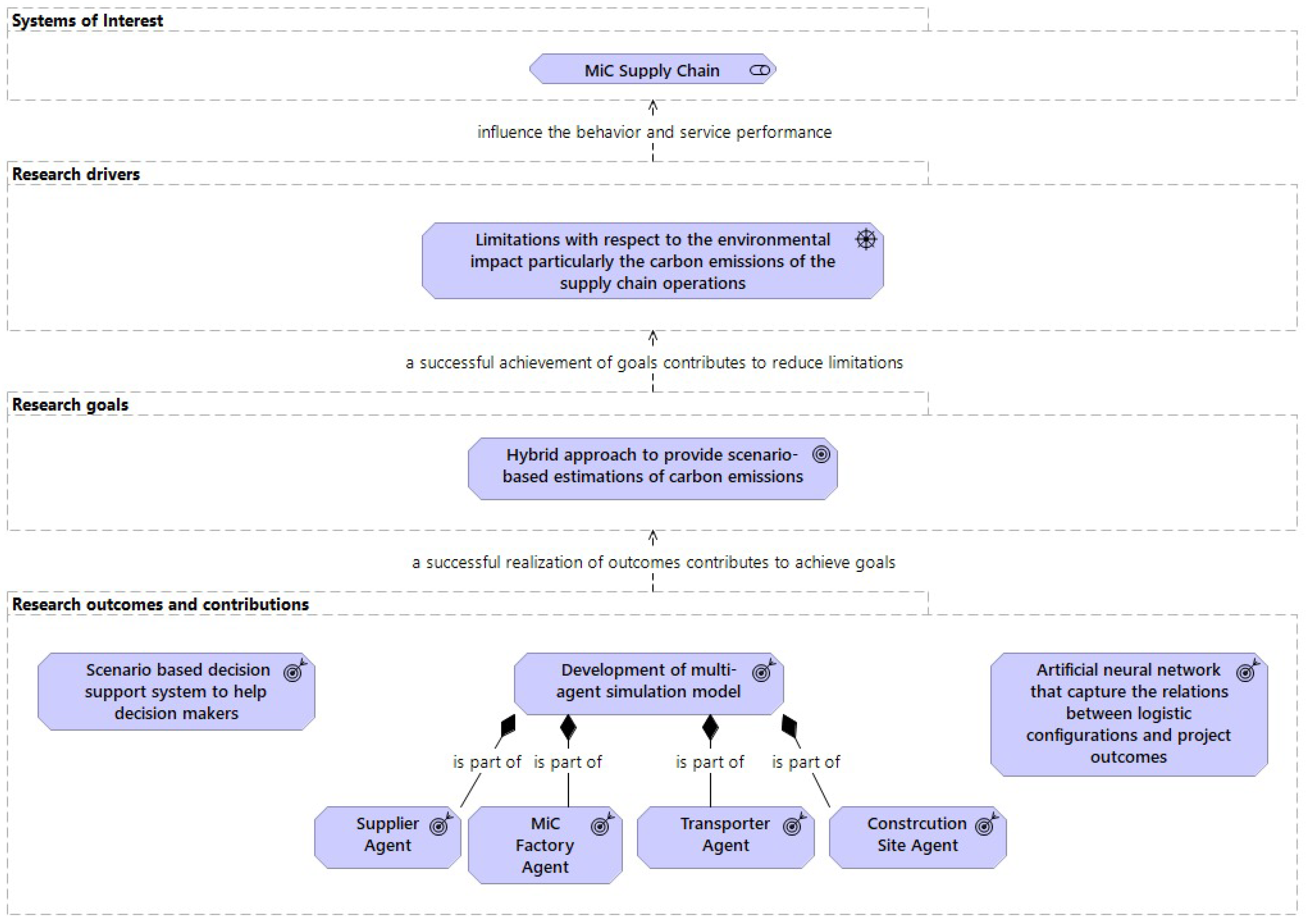
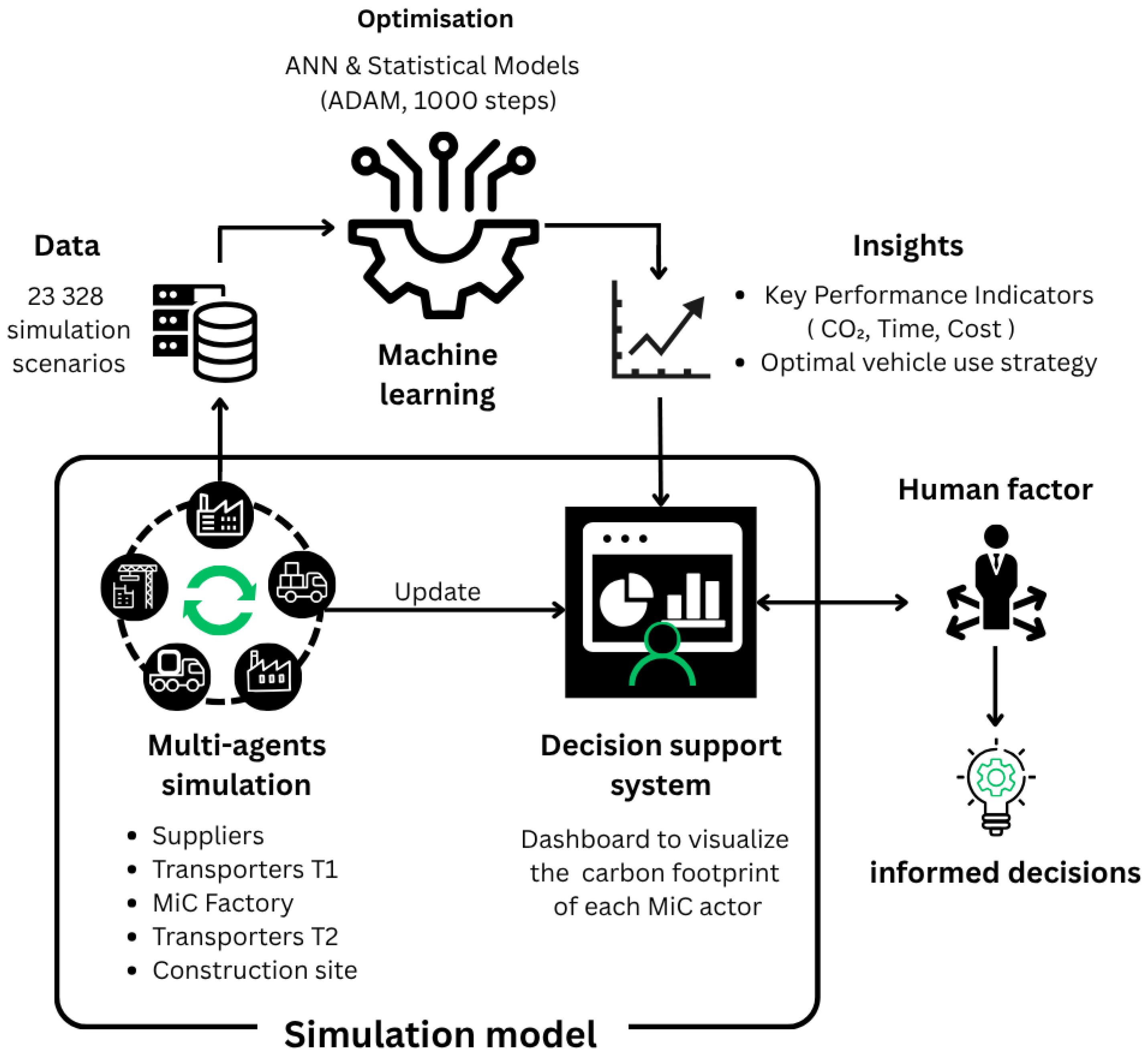
3. Proposed Agent-Based and Machine Learning Optimization Models

In this section, we detail the developed agent-based model that describes MiC configurations. The model leverages AnyLogic’s multi-agent simulation capabilities to efficiently evaluate and optimize the carbon footprint of the MiC supply chain [69]. After that, we describe the machine learning surrogate model generation approach and its application in the optimization of the MiC supply chain. We begin by describing the MiC supply chain problem. Then, we introduce the proposed approach, which consists of the multi-agent simulation framework and the machine learning models used for optimization.

3.1. Problem Description: MiC Supply Chain

The MiC process introduces a modern and more efficient approach to building construction, offering significant opportunities for improving the construction supply chain. Unlike traditional construction methods where the majority of activities occur directly on-site, MiC involves off-site fabrication. Building modules (e.g., rooms, bathroom units, or wall sections) are manufactured in specialized factories and then transported, either fully or partially assembled, to the construction site for final installation. As different phases of construction occur in geographically dispersed locations, effective coordination among these sites becomes crucial. Each step must be carefully planned to prevent delays, minimize inefficiencies, control costs, and reduce environmental impact. The MiC supply chain typically includes three main actors:

• Suppliers: Responsible for producing prefabricated components such as beams, walls, and other structural or architectural elements. These components may vary in type, including concrete, steel, aluminum, and other materials, depending on the design specifications.
• MiC Factories: Prefabricated components from various suppliers are assembled into fully integrated construction modules. These modules are equipped with structural features and also include mechanical, electrical, and plumbing systems. The goal is to produce complete, ready-to-install units that minimize the need for on-site work.
• Construction Sites: Finished modules are received and installed, often with minimal on-site assembly.
• Transporters: These actors are connected through a series of transportation activities. There are two main types of transport activities:

  – 

  From suppliers to MiC factories: This stage uses specialized vehicles tailored to the specific materials being transported. For example, transporting concrete elements may require different vehicles than those used for lighter or more fragile materials like aluminum or glass.

  – 

  From MiC factories to construction sites: This stage involves the movement of fully assembled modules. These modules are often large and delicate, requiring custom vehicles equipped to handle oversized and heavy loads while preventing damage during transit.

The supply chain begins with the movement of prefabricated components from suppliers to factories. After fabrication, the completed modules must then be delivered to the construction sites. This stage requires special transport arrangements because the modules can be large, heavy, and sensitive to damage.

The figure below (Figure 2) presents a simplified view of a typical MiC supply chain. It shows the main entities involved and how materials and modules are moved through the system.

As shown in the figure, all the actors in the MiC supply chain are interconnected and depend on each other. Any effort to improve one part of the system can affect the performance of the entire chain. To build an efficient and sustainable supply chain, we need to find ways to reduce transportation costs and carbon footprint, while still ensuring that deliveries respect the timeline. Finding the right balance between these parameters is key to optimizing the MiC supply chain. Further details regarding these supply chains can be found in our study [70].

3.2. Footprint Carbon in MiC Supply Chain

In this study, we evaluated both the transportation cost and the environmental impact of the MiC supply chain by measuring the carbon footprint associated with each of its main actors. To achieve this, we introduce an important key performance indicator (KPI) that reflect the sustainability of logistics operations, which in this context is the amount of carbon dioxide equivalent ($C{O}_{2}e$) emissions generated throughout the supply chain.

To accurately assess these emissions, we consider specific parameters related to each actor in the supply chain. These parameters are chosen based on their influence on $C{O}_2$ emissions and their relevance to the activities of the respective supply chain actor.

• Suppliers: Suppliers are responsible for producing and delivering prefabricated components, which are often made from a variety of materials such as concrete, steel, or aluminum. Since different materials have different environmental impacts, we base the emissions for this actor primarily on the weight of the components produced. Heavier components usually require more raw materials and energy to manufacture, leading to higher emissions.
  The main factor used to calculate emissions at this stage is the emission factor expressed in kg $C{O}_{2}e$ per kg of material. This value represents the average amount of CO₂e released for each kilogram of material produced.

  $$E^{\sup }=E{F}^{\sup }\times W\times N,$$

  (1)

  where:

  – 

  $E^{\sup }$ = Supplier emissions (kg CO₂e);

  – 

  $E{F}^{\sup }$ = Emission factor per kg of material (kg CO₂e/kg);

  – 

  W = Weight per component (kg);

  – 

  N = Number of components.

  The emission factor can vary depending on the type of material used. For instance, concrete may have a lower emission factor than steel or aluminum, but may still contribute significantly due to its higher usage and weight.
• Transporters: Transporters play a vital role in moving both prefabricated components and finished modules. Emissions in this stage are influenced by the distance traveled and the weight of the transported goods.
  To estimate transport-related emissions, we use an emission factor expressed in kilograms of $C{O}_{2}e$ per kilogram of material transported per kilometer traveled (kg CO₂e/kg · km). This reflects the emissions produced when transporting one kilogram of material over one kilometer.

  $$E^{\mathrm{trans}}=E{F}^{\mathrm{trans}}\times D\times W\times N,$$

  (2)

  where:

  – 

  $E^{\mathrm{trans}}$ = Transport emissions (kg CO₂e);

  – 

  $E{F}^{\mathrm{trans}}$ = Emission factor per kg per km (kg CO₂e/kg · km);

  – 

  D = Distance traveled (km);

  – 

  W = Weight carried (kg);

  – 

  N = Number of modules or components.

  The emission factor can vary depending on the type of transporter. For example, trucks used to transport concrete components need a higher load capacity and consume more fuel than those used to transport lighter materials. In addition, vehicles carrying completed MiC modules that are often too large and delicate require specialized equipment, which can also result in higher emissions.
• MiC Factories: Emissions from MiC factories primarily result from the energy used during the module assembly process. This includes the operation of machines, lighting, heating, and other equipment. These emissions are calculated using the factory’s energy consumption measured in kilowatt-hours (kWh), multiplied by an appropriate emission factor (kg CO₂e/kWh).

  $$E^{\mathrm{fact}}=E{F}^{\mathrm{fact}}\times P\times T\times N,$$

  (3)

  where:

  – 

  $E^{\mathrm{fact}}$ = Factory emissions (kg CO₂e);

  – 

  $E{F}^{\mathrm{fact}}$ = Emission factor per kWh (kg CO₂e/kWh);

  – 

  P = Power consumption per module (kW);

  – 

  T = Fabrication time (hours);

  – 

  N = Number of modules.

• Construction Sites: While the construction site activities are relatively limited in MiC projects, there are still emissions related to on-site energy usage. These may include crane operations, minor installations, and lighting or heating during final assembly. Similar to the factory, emissions here are based on energy consumption.

  $$E^{\mathrm{site}}=E{F}^{\mathrm{site}}\times P\times T\times N,$$

  (4)

  where:

  – 

  $E^{\mathrm{site}}$ = Site emissions (kg CO₂e);

  – 

  $E{F}^{\mathrm{site}}$ = Emission factor per kWh (kg CO₂e/kWh);

  – 

  P = Power consumption per module (kW);

  – 

  T = Operational time (hours);

  – 

  N = Number of modules.

• Total Carbon Footprint: At the end of the evaluation process, the emissions calculated for each actor in the supply chain are summed to determine the total carbon footprint of the entire MiC supply chain. This aggregated value gives a complete picture of the environmental impact from raw-material supply through final on-site installation:

  $$\mathrm{Total}\mathrm{CF}=\sum _{i=1}^{N_S}{E}_i^{\sup }+\sum _{k=1}^{N_T}{E}_k^{\mathrm{trans}}+\sum _{j=1}^{N_F}{E}_j^{\mathrm{fact}}+\sum _{c=1}^{N_{CS}}{E}_c^{\mathrm{site}}.$$

  (5)
  Here:

  – 

  $E_i^{\sup }$ = Emissions from supplier i;

  – 

  $E_k^{\mathrm{trans}}$ = Emissions from transporter k;

  – 

  $E_j^{\mathrm{fact}}$ = Emissions from factory j;

  – 

  $E_c^{\mathrm{site}}$ = Emissions from construction site c;

  – 

  $N_S,N_T,N_F,N_{CS}$ = Number of suppliers, transporters, factories, and construction sites, respectively.

In addition to carbon emissions, another important performance indicator considered in this study is the transportation cost. This indicator specifically applies to the transporter actors and reflects the financial aspect of moving components and modules between sites. Detailed information regarding how transportation costs are calculated and analyzed is taken from our previous study [70].

3.3. Proposed Approach

In this section, we detail the developed agent-based model (ABM) and the machine learning approach. The ABM exploits AnyLogic’s multi-agent simulation capabilities to efficiently assess MiC supply chain $C{O}_2$ emissions.

3.3.1. Modeling of Interactions Between Agents

The sequence diagram below (Figure 3) provides a detailed and easy-to-follow view of the full process involved in an MiC supply chain. It shows how different agents like the construction site, MiC factory, component supplier, two transport teams (Transporter T1 and T2), and a decision support system work together step by step to complete a construction project. Each stage in the process is carefully organized, and the diagram helps explain how the flow of materials, communication, and decisions happens from start to finish.

The process begins when the construction site generates a demand for construction modules. This request is sent to the MiC factory, which then generates its own demand for the components needed to build those modules. The factory sends a request to the supplier to provide these components. Once the supplier receives the request, they start producing the components. After production, the supplier calculates the carbon emissions from their activities and sends a request for transportation.

Transporter T1 is assigned to pick up and deliver these components to the factory. The components are loaded by Transporter T1 and delivered to the MiC factory. During this phase, carbon emissions from Transporter T1 are also calculated. As the components arrive, the MiC factory begins the process of fabricating the integrated construction modules. The emissions created during this production stage are also tracked and calculated.

Once the modules are completed, the MiC factory requests transport again this time from Transporter T2 to deliver the finished modules to the construction site. The modules are loaded and transported by Transporter T2, with another carbon emission calculation performed for this delivery process.

When the modules arrive at the construction site, on-site assembly begins. The emissions generated at this stage are calculated as well. After the modules are assembled into the final structure, the construction site notifies the factory that the work is complete, and the decision support system is updated one last time with key performance indicators.

Throughout the entire process, the decision support system plays a crucial role by collecting and updating information at key points, such as after production, each delivery, and at the end of assembly. It uses this data to calculate carbon emissions and update performance metrics.

In the parameter selection section of the case study described below, we considered a configuration involving five suppliers and one MiC factory, forming the baseline setup for our simulation experiments. To systematically explore the performance of different supply chain configurations, we conducted a parameter variation experiment using AnyLogic’s built-in experimentation tools. Specifically, we varied the number of vehicles allocated to each of the five suppliers from 1 to 6, and the number of vehicles at the MiC factory from 1 to 3. This resulted in a full factorial design comprising $6^5\times 3$ = 23,328 unique simulation scenarios. Each scenario represents a distinct combination of vehicle allocations, and for each, the multi-agent system generated detailed outputs including completion time, transportation costs, fixed and variable costs, penalty costs, and carbon footprint. Each scenario was executed under the same model structure, but due to the use of uniform distributions in several stochastic parameters which led to natural replications across different runs with the same configuration, thereby reflecting the realistic variability.

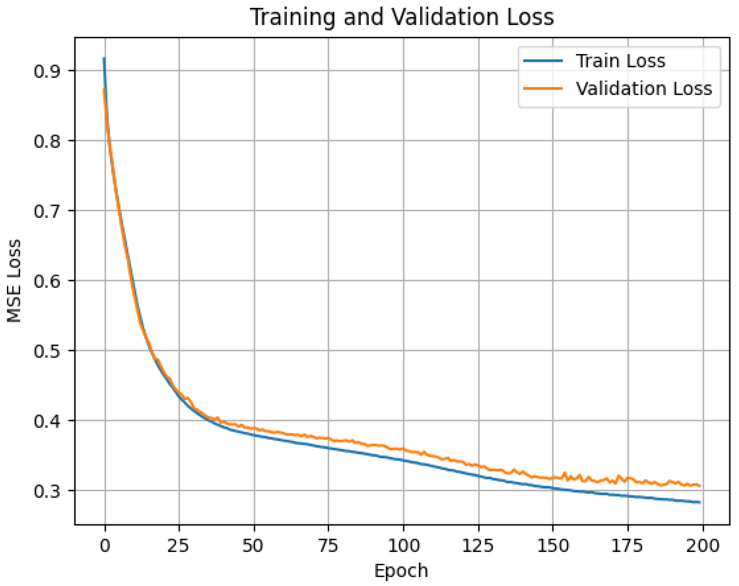
3.3.2. Machine Learning Surrogate Models for Supply Chain Optimization

After developing the multi-agent model, we executed more than 23,000 simulation scenarios and collected key data, such as the number of vehicles used by suppliers and factories. We also recorded important project KPIs, including project completion time, total transport cost, and $C{O}_2$ emissions for each scenario.

We use an artificial neural network (ANN) to predict and optimize the total $C{O}_2$ emissions, the completion time, and the total cost. The inputs consist of the number of vehicles used by suppliers and factories. The ANN comprises a series of dense layers and three outputs. The most accurate architecture was determined through trial and error by increasing the number of nodes and layers until good accuracy was achieved and to prevent overfitting. The hidden layers consist of $12\times 24\times 64\times 256\times 48\times 12\times 6$. The ReLU activation function was used for all nodes in the hidden layers [71]. The ADAM optimization algorithm was used to fit the weights of the nodes [72]. A learning rate of 0.0001 was chosen to balance learning speed and convergence stability. The libraries TensorFlow and Keras were used for the training [73,74].

The simulation data points were divided into training and validation datasets, with the training set representing 70% of the total data. Scaling was applied to all features and outputs to ensure that their relative contributions were appropriately captured. The learning process consisted of 200 epochs with a batch size of 25, and the mean squared error (MSE) was used as the loss function. The evolution of the validation and testing loss functions is shown in Figure 4. The final validation MSEs after training were estimated at:

• MSE for total carbon footprint (in kg CO₂e): 481,689,693.30;
• MSE for completion time (in days): 20.45;
• MSE for total cost (in EUR): 529,124,195.93.

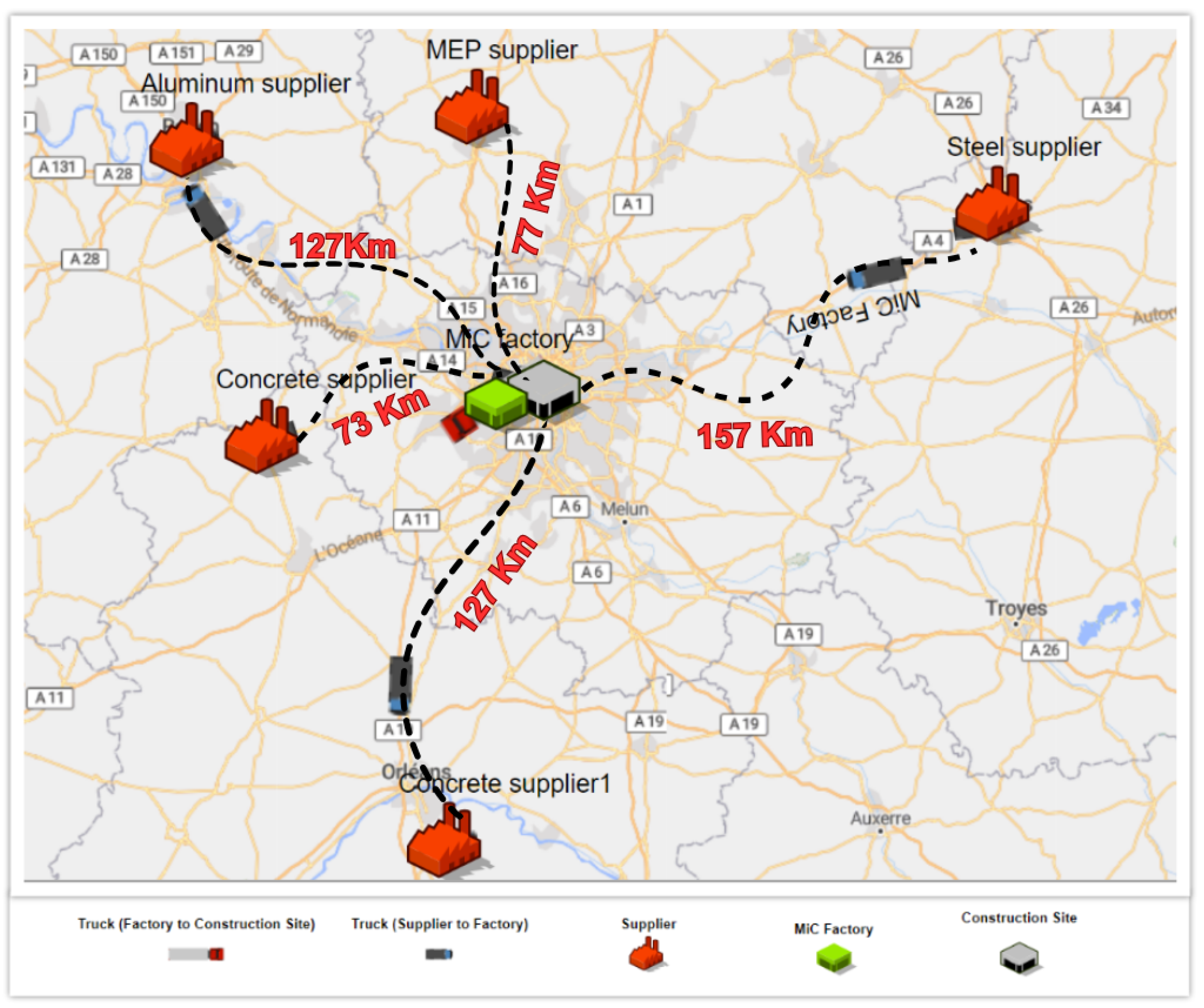
In addition to the artificial neural network, we trained and evaluated four statistical learning algorithms known for their predictive accuracy (

Table 2. Mean squared errors (MSEs) for different statistical learning models on predicting $\mathit{C}{\mathit{O}}_2$ emissions, completion time, and cost on the validation dataset.

Model	MSE (${\mathit{CO}}_2$)	MSE (Time)	MSE (Cost)
SVM (SVR)	541,352,400.00	39.32	398,188,700.00
Random Forest	589,882,000.00	0.29	239,012,000.00
Gradient Boosting	496,780,700.00	82.00	5,397,325,000.00
XGBoost	508,183,300.00	0.22	81,027,600.00

). The first was the support vector regressor (SVR) [75], with a regularization parameter set to 100. SVR ranked third in predicting $C{O}_2$ emissions, completion time, and cost. While it outperformed the neural network in cost prediction, it underperformed in the other two metrics. The second model was a random forest with 100 decision trees [76]. It ranked second for both completion time and cost, but last in $C{O}_2$ prediction. The third algorithm, gradient boosting with 100 estimators [77], achieved the best performance in predicting $C{O}_2$ emissions but was the least accurate in determining the time and the cost. Finally, XGBoost [78], also with 100 estimators, delivered the most accurate predictions for completion time and cost, and ranked third in $C{O}_2$ estimation. The scikit-learn library was used for the implementation and training of these four algorithms [79].

Next, we took advantage of the low computational cost of the trained ANN to optimize the vehicle distribution among suppliers and MiC factories to ensure optimal construction strategies that minimize the total carbon footprint, the completion time, and total cost. We solve the following discrete optimization algorithm:

$$\begin{array}{cc}\hfill \mathrm{Minimize}:& \mathrm{model}\left(\mathbf{x}\right)=\alpha ·C{O}_2+\beta ·\mathrm{Time}+\gamma ·\mathrm{Cos}\mathrm{t}.\hfill \end{array}$$

where $C{O}_2$, Time, and Cost represent the normalized predicted carbon footprint, completion time, and total cost, respectively. The weights $\alpha$, $\beta$, $\gamma$ will be varied to describe strategies that minimize one or several outputs. The values of these weight parameters are chosen so that the total is always equal to 1 and each value of each weight indicates the percent of prioritization given to each strategy. Furthermore, $x={\left(x_i\right)}_i$, with $x_i$ represents the number of vehicles used by suppliers and MiC factories. We use the ADAM optimization algorithm to solve this problem [72]. To ensure convergence, we use 1000 steps for the resolution. The total resolution time is estimated at 7.54 s. The code and data are available publicly accessible at https://github.com/MPS7/construction_ML_study (accessed on 11 April 2025).

To visually summarize the workflow and interaction between components of the proposed framework, Figure 5 presents an integrated decision-making loop. This diagram captures the iterative process in which simulation agents generate data based on MiC supply chain scenarios. These data feed into machine learning models, which are trained to predict key performance indicators such as cost, carbon emissions, and project duration. The trained surrogate models support rapid multi-objective optimization, and the resulting insights are passed to a decision support system. This system facilitates informed decision making by human stakeholders, closing the loop and enabling continuous scenario evaluation and system refinement.

4. Case Study

To simulate the MiC supply chain, a multi-agent model was implemented using AnyLogic. This simulation includes various agents representing different elements of the supply chain and follows a structured workflow that mirrors real-world operations.

4.1. Agents Description

The model includes different types of agents, each with a specific role in the MiC supply chain. These agents interact with each other to reflect how materials, components, and information move in real construction projects. The following list briefly explains the role of each agent in the simulation.

• Construction site: Generates demand for modules based on BIM data and project schedules. It initiates requests for integrated modules.
• MiC factory: Handles the reception of orders, fabrication of integrated modules, and assignment of vehicles for delivery to construction sites.
• Suppliers: Responsible for producing and delivering prefabricated components to the MiC factory. Each supplier has parameters such as production rate, storage capacity, and vehicle availability. In our case study, we used a total of five suppliers, divided into four categories: two for concrete wall panels, one for steel beams, one for MEP components, and one for aluminum frames.
• Transporters:

  – 

  T1: Transports components from suppliers to the MiC factory.

  – 

  T2: Transports completed modules from the MiC factory to construction sites.

  Both are managed using state charts to simulate the loading, traveling, unloading, and returning cycles.

The main agent integrates all agents and simulates a realistic logistics network using a GIS map, built with OpenStreetMap (OSM) data. This map includes actual locations, transportation routes, and distances between agents.

4.2. Parameter Selection

The parameters adopted in this simulation reflect the operational constraints and logistics characteristics commonly observed in mid-sized modular integrated construction (MiC) projects. The number of suppliers, types of vehicles, production capacities, and associated costs were selected based on both industry standards and relevant academic literature to ensure realism and reliability. Supplier selection was guided by the core categories of materials and systems essential to MiC, including concrete, steel, aluminum, and MEP components—representing the fundamental inputs for prefabricated module fabrication. Although each direct supplier may rely on its own upstream network, we adopted a simplifying assumption by focusing solely on immediate suppliers to streamline the model and emphasize primary logistics flows. Vehicle allocation ranges were determined based on typical fleet configurations and operational variability documented in case studies, enabling the simulation to capture practical supply chain strategies while remaining computationally tractable. Cost parameters, including fixed and variable transportation costs and delay penalties, were based on typical economic considerations (Trucking Dive, https://www.truckingdive.com/ accessed 30 May 2024). Stochastic elements, such as vehicle speeds and production rates, were integrated to reflect real-world uncertainties and variability in transport and manufacturing processes. Emission data was collected from reliable sources (e.g., the climatiq database [80]), which provides reliable, up-to-date emission factors. In addition, scientific literature was consulted [81] to further examine the data. This data includes emissions from materials, transportation, and energy consumption at different stages of the supply chain.

Table 3. A summary of parameters used in the MiC multi-agent simulations and their values.

Parameter	Value	Unit	Description
Project Setup
Number of Suppliers	5	-	Suppliers providing prefabricated components
Number of MiC Factories	1	-	Centralized factory for module assembly
Construction Site Location	Paris, France	-	Location of final module installation
Normal Project Completion Time	120	days	Deadline to avoid penalty
Production and Storage
Avg. Requests per Day	60 C, 3 M	C: Components, M: Modules	Daily component/module demand
Initial Storage per Supplier	uniform(5, 10)	Components	Initial buffer stock
Production Capacity (Supplier)	uniform(10, 15)	Components/day	Daily component production
Production Capacity (Factory)	uniform(3, 5)	Modules/day	Daily module output
Logistics and Transportation
Vehicles (T1) per Supplier	[1,2,3,4,5,6]	vehicles	Vehicles used to transport components
Vehicles (T2) per Factory	[1,2,3]	vehicles	Vehicles used to deliver assembled modules
Vehicle Speed T1	uniform(50, 70)	km/h	Speed range for component delivery
Vehicle Speed T2	uniform(40, 60)	km/h	Speed range for module delivery
Fixed Cost T1	150	EUR/day	Daily fixed cost for T1 vehicles (e.g., rental, driver salary, insurance)
Fixed Cost T2	200	EUR/day	Daily fixed cost for T2 vehicles (e.g., rental, driver salary, insurance)
Variable Cost T1	2	EUR/km	Per-kilometer variable cost for T1 (e.g., fuel, maintenance, tire wear)
Variable Cost T2	3	EUR/km	Per-kilometer variable cost for T2 (e.g., fuel, maintenance, tire wear)
Project Delay Penalty	500	EUR/day	Penalty for late delivery
Supplier Locations to MiC Factory	Supplier1: uniform(70, 75), Supplier2: uniform(125, 130), Supplier3: uniform(155, 160), Supplier4: uniform(75, 80), Supplier5: uniform(125, 130)	km	Distance from suppliers to factory
Factory to Site Distance	uniform(20, 22.5)	km	Transport distance for modules
Energy and Emissions
Energy Emission Factor	uniform(0.039, 0.4041)	kg CO2e/kWh	Emissions per energy unit
Fabrication Energy Use	uniform(13, 70)	kW	Energy required for assembly
Fabrication Time	uniform(2, 3)	hours	Time to assemble one module
Construction Energy Use	uniform(65, 300)	kW	Energy used during site work
Construction Time	uniform(0.1, 1)	hours	Time for on-site installation
Material Details
Concrete Emission Factor	uniform(0.17, 0.27)	kg CO2e/kg	Concrete emission rate based on the weight
Steel Emission Factor	uniform(0.5, 0.7)	kg CO2e/kg	Steel emission rate based on the weight
Insul. + MEP Emission Factor	uniform(10.3, 11.45)	kg CO2e/kg	Insulation with MEP emission rate based on the weight
Aluminum Emission Factor	uniform(1.4, 3.85)	kg CO2e/kg	Aluminum emission rate based on the weight
Concrete Weight	uniform(2400, 7700)	kg	Weight of prefabricated concrete
Steel Weight	uniform(457.2, 2880)	kg	Weight of steel beams
Insul. + MEP Weight	uniform(14, 17)	kg	Weight of internal MEP units
Aluminum Weight	uniform(1.62, 108.00)	kg	Weight of aluminum units
Module Weight	uniform(21,091, 73,616)	kg	Assembled module weight
Transportation Emissions
Concrete Transport Factor	uniform(0.000062, 0.000256)	kg CO2e/kg · km	Emission rate for concrete freight
Steel Transport Factor	uniform(0.000088, 0.000363)	kg CO2e/kg · km	Emission rate for steel freight
MEP+Aluminum Transport Factor	uniform(0.00012, 0.00015)	kg CO2e/kg · km	Emission rate for MEP/Aluminum freight
General Freight Factor	uniform(0.00005, 0.00006)	kg CO2e/kg · km	Baseline freight emissions

summarizes all the key parameters used in the simulation, covering supply chain configuration, transportation, energy consumption, emissions, and project logistics.

4.3. Simulation Results

In the simulation, suppliers deliver prefabricated components to MiC factories, which then send fully assembled construction modules to the construction site. Figure 6 shows the GIS-based map from AnyLogic, where the locations of suppliers, the MiC factory, and the construction site are clearly displayed.

The distances and routes illustrated in Figure 6 are not straight-line measurements, but rather realistic road distances automatically computed using the GIS mapping capabilities of AnyLogic. This tool calculates travel paths based on the actual road network infrastructure, providing a more accurate representation of transportation routes. Consequently, the resulting estimates for travel time, transportation cost, and carbon footprint better reflect real-world logistics conditions.

Table 4. Results for multi-agent simulations that consider varying numbers of vehicles per supplier and MiC factory.

Vehicles per Supplier	Vehicles per MiC factory	Var. Cost T1 (EUR)	Var. Cost T2 (EUR)	Fixed Cost T1 (EUR)	Fixed Cost T2 (EUR)	Project Time (Days)	Penalty (EUR)	Total Cost (EUR)	Carbon Footprint (kg ${\mathit{CO}}_2\mathit{e}$)
1	1	1,648,941	46,042	219,100	58,427	292	86,067	2,058,576	3,816,959
1	2	1,648,806	45,974	219,430	117,029	293	86,286	2,117,525	3,796,678
1	3	1,649,246	46,254	219,349	175,479	292	86,233	2,176,560	3,769,565
2	1	1,648,691	46,066	219,560	29,275	146	13,187	1,956,778	3,806,080
2	2	1,649,390	46,010	219,736	58,596	146	13,245	1,986,978	3,834,559
2	3	1,648,785	45,979	218,550	87,420	146	12,850	2,013,585	3,802,363
3	1	1,649,603	45,994	219,583	19,518	98	0	1,934,699	3,787,588
3	2	1,649,795	46,039	220,150	39,138	98	0	1,955,123	3,814,929
3	3	1,649,388	45,994	220,024	58,673	98	0	1,974,079	3,805,549
4	1	1,649,598	46,024	242,550	16,170	81	0	1,954,342	3,816,099
4	2	1,649,555	46,092	242,505	32,334	81	0	1,970,486	3,786,941
4	3	1,649,472	46,063	242,569	48,514	81	0	1,986,618	3,766,033
5	1	1,649,060	46,045	303,118	16,166	81	0	2,014,389	3,805,143
5	2	1,648,942	46,095	303,127	32,334	81	0	2,030,498	3,800,661
5	3	1,649,147	45,972	303,072	48,492	81	0	2,046,683	3,795,932
6	1	1,649,559	46,035	363,737	16,166	81	0	2,075,496	3,797,855
6	2	1,649,520	46,092	363,725	32,331	81	0	2,091,669	3,811,072
6	3	1,649,001	45,944	363,727	48,497	81	0	2,107,169	3,789,590

presents the results of the simulation. It shows the variation in total cost and carbon footprint for different combinations of vehicles used by suppliers and the MiC factory. The results help identify the optimal combination that minimizes total cost and environmental impact while ensuring timely project delivery.

The variable costs for the transportation process are divided between T1 and T2 (transporters 1 and 2). From the data presented in the table, we can observe that the variable costs for both T1 and T2 remain stable across different configurations, indicating that the system’s routing efficiency does not fluctuate significantly with the number of vehicles. This suggests that the variable cost per trip is largely unaffected by the number of vehicles used.

In contrast, the fixed costs for both T1 and T2 show a clear pattern in response to the number of vehicles deployed. As the number of vehicles per supplier increases, the total fixed cost for T1 rises, starting from EUR 219,100 and gradually increasing with more vehicles, peaking at EUR 363,737 when six vehicles are deployed. Similarly, the fixed cost for T2 increases with the number of vehicles, and it is particularly influenced by the number of T1 vehicles. When the number of T1 vehicles is low, the fixed costs for T2 rise due to the increased time required for T2 to deliver the modules. This is further compounded by the fact that the total fixed cost is impacted by the overall project completion time, as the longer the project duration, the higher the costs associated with resources and logistics.

The penalty costs are primarily affected by the number of vehicles allocated to T1 suppliers. When only one vehicle is assigned to each supplier, the penalty costs are notably higher, reflecting substantial delays in transportation and project scheduling. As the number of vehicles increases, the penalty costs decrease progressively. Notably, once three or more vehicles per supplier are introduced, the penalty costs disappear entirely, suggesting that having additional vehicles alleviates operational delays. This improves the efficiency of delivery, which ultimately enhances project scheduling and reduces overall penalty costs.

When examining the carbon footprint, the table demonstrates that the total emissions are relatively unaffected by the number of vehicles used. The total carbon footprint remains stable across different configurations, hovering around 3.8 million kg CO₂e. This stability indicates that, despite the increase in the number of vehicles, the emissions associated with transportation are relatively minor compared to other sources in the supply chain. In particular, emissions produced by the suppliers themselves, especially during the production of the prefabricated components, are likely the primary contributors to the carbon footprint.

This observation suggests that transport emissions, while contributing to the overall carbon footprint, do not drastically alter the environmental impact when varying the number of vehicles. The overall operational emissions are primarily driven by the activities at the suppliers, rather than the transport phase of the process.

For instance, the carbon footprint of the construction process shows little variation, regardless of whether one, two, or six vehicles per supplier are used. This suggests that the system is not highly sensitive to transportation changes, and that the overall environmental impact would be more significantly affected by alterations in the supply chain configuration, such as the number of suppliers or the types of materials used in the prefabrication process. Figure 7 presents the breakdown of carbon emissions across the different stages of the MiC supply chain.

The results show that the majority of carbon emissions, over 80%, is generated by the suppliers. Transport activities, which include the delivery of components from suppliers to the factory and from the factory to the construction site, account for around 14% of the total emissions. Meanwhile, activities at the MiC factory and at the construction site contribute very little to the overall carbon footprint, each representing approximately 1% of the total.

This indicates that the way materials are produced has a much greater impact on the environment than how they are transported or assembled at factories and on-site.

Looking more closely at the suppliers’ contribution, it is clear that concrete suppliers are responsible for the largest share of emissions, making up about 65% of the total. Steel suppliers are the next biggest contributors, with around 27%. Other suppliers, such as those providing MEP systems and aluminum parts, have a much smaller impact, with shares of 5% and 3%, respectively.

This analysis suggests that efforts to reduce the carbon footprint of modular construction should focus primarily on the choice of materials and improvements at the supplier level. Selecting lower-carbon alternatives or optimizing material usage could significantly reduce the overall environmental impact of the construction project.

4.4. Optimal Supply Chain Strategies for Sustainable, Cost-Effective, and/or Fast Construction

We leveraged the low computational cost of the ANN surrogate model to evaluate strategies aimed at minimizing carbon footprint, completion time, and total cost. Although all algorithms did relatively well (Appendix A), we choose to present the results obtained by the ANN because (i) the high number of generated data allowed us to train the ANN and (ii) other algorithms might display cases of overfitting when trained on large datasets. The TensorFlow optimization suite was used to identify supply chain configurations that achieve optimal performance, along with their corresponding predicted $C{O}_2$ emissions, completion times, and costs. The resulting strategies are summarized in

Table 5. The predicted optimal strategies minimize weighted combinations of carbon footprint ($\alpha$), completion time ($\beta$), and total cost ($\gamma$). The target values for each strategy were estimated using the artificial neural network trained based on the MAS results.

$\mathit{\alpha }$	$\mathit{\beta }$	$\mathit{\gamma }$	Strategy	Carbon Footprint (kg CO2e)	Project Time (Days)	Total Cost (EUR)
1	0	0	[1 6 1 2 1 3]	3,776,432.50	288.79	2,392,895.50
0	1	0	[3 5 5 6 5 3]	3,791,940.50	82.67	2,036,646.38
0	0	1	[3 5 3 4 1 1]	3,777,434.00	99.66	1,948,504.75
0.33	0.33	0.33	[3 5 3 4 1 1]	3,781,251.00	90.76	1,960,009.00
0.5	0.5	0	[5 1 6 6 6 3]	3,772,361.00	260.93	2,712,012.50
0.5	0	0.5	[3 6 5 5 2 1]	3,797,530.50	123.04	2,099,554.50
0	0.5	0.5	[3 5 5 3 4 1]	3,791,096.50	118.98	2,038,015.88

. The strategy that minimizes carbon footprint involves assigning more vehicles to the second concrete wall supplier, fewer vehicles to the steel beam, MEP, and aluminum suppliers, and the maximum number to the MiC factory. This strategy results in the emission of 3,777,434.00 kg CO₂e. The fastest strategy, in terms of completion time, requires a high number of vehicles across all suppliers and the MiC factory. It achieves a predicted project duration of approximately 82.67 days. The most cost-effective strategy involves assigning a moderate-to-high number of vehicles to the concrete, steel beam, and MEP suppliers, while minimizing allocation to the aluminum supplier and the MiC factory. This strategy reduces the cost to roughly 1,948,504.75 EUR.

We extended our analysis by evaluating strategies that minimize multiple objectives simultaneously. The strategy that minimizes carbon footprint, completion time, and total cost involves assigning a high number of vehicles to all suppliers except the second concrete supplier, and allocating the maximum number of vehicles to the MiC factory. Notably, this strategy results in a lower $C{O}_2$ emission level than the strategy optimized solely for carbon footprint. The strategy that minimizes both carbon footprint and completion time requires a high number of vehicles for all suppliers, except one of the concrete suppliers, and also assigns the maximum number of vehicles to the MiC factory. Meanwhile, the strategy that optimizes carbon footprint and total cost consists of allocating an average to high number of vehicles to all suppliers except the aluminum supplier, while assigning only one vehicle to the MiC factory. The optimal strategies provided by the support vector regressor, the random forest, the gradient boosting, and the XGboost algorithms were similar to the ones provided by the deep learning algorithm as shown in

Table A1. Optimization results using the support vector regressor model for different weight combinations of $\alpha$, $\beta$, and $\gamma$.

$\mathit{\alpha }$	$\mathit{\beta }$	$\mathit{\gamma }$	Strategy	Carbon Footprint (kg CO2e)	Project Time (Days)	Total Cost (EUR)
1.00	0.00	0.00	[1, 6, 1, 2, 1, 3]	3,784,115.73	294.06	2,443,178.13
0.00	1.00	0.00	[3, 5, 5, 6, 5, 3]	3,798,058.77	77.22	2,015,068.14
0.00	0.00	1.00	[3, 5, 3, 5, 4, 1]	3,783,287.56	88.18	1,951,318.48
0.33	0.33	0.34	[3, 5, 3, 3, 4, 1]	3,787,855.40	94.04	1,967,158.35
0.50	0.50	0.00	[5, 1, 6, 6, 6, 3]	3,758,459.58	252.42	2,836,372.95
0.50	0.00	0.50	[3, 6, 5, 5, 2, 1]	3,783,672.58	126.26	2,117,662.12
0.00	0.50	0.50	[3, 5, 5, 3, 4, 1]	3,781,124.36	81.88	1,955,009.28

,

Table A2. Optimization results using the random forest model for different weight combinations of $\alpha$, $\beta$, and $\gamma$.

$\mathit{\alpha }$	$\mathit{\beta }$	$\mathit{\gamma }$	Strategy	Carbon Footprint (kg CO2e)	Project Time (Days)	Total Cost (EUR)
1.00	0.00	0.00	[1, 6, 1, 2, 1, 3]	3,770,827.21	292.37	2,450,530.52
0.00	1.00	0.00	[3, 5, 5, 6, 5, 3]	3,796,971.18	80.83	2,036,033.15
0.00	0.00	1.00	[3, 5, 3, 5, 4, 1]	3,785,973.25	86.90	1,950,204.44
0.33	0.33	0.34	[3, 5, 3, 3, 4, 1]	3,781,343.71	97.63	1,975,610.88
0.50	0.50	0.00	[5, 1, 6, 6, 6, 3]	3,804,725.82	260.12	2,809,141.08
0.50	0.00	0.50	[3, 6, 5, 5, 2, 1]	3,793,755.45	126.32	2,120,010.58
0.00	0.50	0.50	[3, 5, 5, 3, 4, 1]	3,780,677.81	80.85	1,959,081.14

,

Table A3. Optimization results using the gradient boosting model for different weight combinations of $\alpha$, $\beta$, and $\gamma$.

$\mathit{\alpha }$	$\mathit{\beta }$	$\mathit{\gamma }$	Strategy	Carbon Footprint (kg CO2e)	Project Time (Days)	Total Cost (EUR)
1.00	0.00	0.00	[1, 6, 1, 2, 1, 3]	3,798,056.88	292.93	2,529,926.56
0.00	1.00	0.00	[3, 5, 5, 6, 5, 3]	3,794,873.51	93.73	2,128,785.70
0.00	0.00	1.00	[3, 5, 3, 5, 4, 1]	3,785,240.99	96.61	2,065,890.33
0.33	0.33	0.34	[3, 5, 3, 3, 4, 1]	3,786,759.29	104.25	2,067,947.50
0.50	0.50	0.00	[5, 1, 6, 6, 6, 3]	3,789,078.95	246.00	2,677,288.01
0.50	0.00	0.50	[3, 6, 5, 5, 2, 1]	3,788,573.06	123.99	2,117,511.81
0.00	0.50	0.50	[3, 5, 5, 3, 4, 1]	3,788,060.45	93.73	2,089,791.47

and

Table A4. Optimization results using the XGBoost model for different weight combinations of $\alpha$, $\beta$, and $\gamma$.

$\mathit{\alpha }$	$\mathit{\beta }$	$\mathit{\gamma }$	Strategy	Carbon Footprint (kg CO2e)	Project Time (Days)	Total Cost (EUR)
1.00	0.00	0.00	[1, 6, 1, 2, 1, 3]	3,766,735.25	292.47	2,437,129.75
0.00	1.00	0.00	[3, 5, 5, 6, 5, 3]	3,798,643.75	80.86	2,037,618.13
0.00	0.00	1.00	[3, 5, 3, 5, 4, 1]	3,789,310.50	86.95	1,951,549.75
0.33	0.33	0.34	[3, 5, 3, 3, 4, 1]	3,785,677.75	97.54	1,973,190.88
0.50	0.50	0.00	[5, 1, 6, 6, 6, 3]	3,791,028.25	260.17	2,851,382.00
0.50	0.00	0.50	[3, 6, 5, 5, 2, 1]	3,789,575.25	126.36	2,120,164.75
0.00	0.50	0.50	[3, 5, 5, 3, 4, 1]	3,788,197.75	80.77	1,956,994.50

of Appendix A.

4.5. Discussion

This work examines the impact of supply chain configurations on carbon emissions in MiC frameworks. We developed a multi-agent model representing the MiC supply chain. The model includes suppliers, an MiC factory, construction sites, and a transportation fleet, with each component modeled as an autonomous agent. We estimated process and transportation emissions using emission factors expressed in kilograms of $C{O}_2$. The model was adapted to a case study simulating realistic logistics using a GIS map, incorporating actual locations, transportation routes, and distances between agents. Model parameters were informed by economic and technical documents, emission data, and scientific literature relevant to mid-sized construction projects.

We used numerical simulations to study a range of construction scenarios. The results suggest that changes in vehicle allocation strategies influence the fixed costs associated with transportation, but not the variable costs. This is because the number of vehicles regulates the completion time, which directly impacts fixed costs. Penalty costs were more sensitive to the number of vehicles allocated to T1 suppliers. Regarding carbon footprints, the simulations predict that $C{O}_2$ emissions from transportation contribute only minimally to the overall carbon footprint. This indicates that reducing total emissions would require more significant changes, such as altering the number of suppliers or the types of materials used in the prefabrication process.

Figure 8a presents a heatmap showing how total cost varies across different combinations of vehicles assigned to suppliers and the MiC factory. This visualization clearly illustrates that increasing the number of vehicles generally leads to lower penalty costs, thereby reducing total cost. Figure 8b further reinforces this insight with a 3D surface plot that captures the non-linear interactions between vehicle allocations and total cost.

Moreover, Figure 9 demonstrates that carbon footprint remains relatively invariant across different vehicle configurations. This observation supports our prior claim that logistics-related emissions are marginal contributors compared to prefabrication and material processes.

Given the complex, stochastic, and high-dimensional nature of MiC logistics planning, conventional optimization methods such as linear programming or rule-based heuristics often fall short in capturing the dynamic interdependencies and decentralized decision making typical of construction supply chains. MAS offer a compelling alternative by enabling the explicit modeling of heterogeneous agents, each with their own objectives, behaviors, and constraints. This agent-based representation allows for a more realistic simulation of logistical complexity, including asynchronous interactions, decentralized control, and spatially distributed operations.

However, this expressiveness comes at a computational cost. MAS simulations require significant CPU resources and time, particularly when exploring large-scale strategy spaces or running multiple stochastic replications for robustness. To overcome these limitations and improve usability for decision makers, we developed a hybrid framework that combines MAS with machine learning surrogate models.

The surrogate models were trained to emulate the outputs of the MAS, offering two main advantages: (i) A substantial reduction in computational time—transforming simulations that take hours into milliseconds—and (ii) the ability to embed the surrogate within multi-objective optimization routines to explore trade-offs under various constraints. Similar approaches have been used to evaluate the impact of urban expansion on the microclimate [82].

We implemented a comparative analysis using several well-established regression algorithms, including artificial neural networks (ANN), support vector regressors (SVR), random forest (RF), gradient boosting (GB), and XGBoost. All trained models predicted the outputs with good accuracy. The predictions made by the artificial neural network aligned closely with the simulation results of the multi-agent framework. Specifically, employing a larger number of vehicles led to faster completion times and lower total costs, without significantly affecting $C{O}_2$ emissions. Strategies that minimized cost were associated with using fewer vehicles at the MiC factory. In contrast, strategies that minimized the carbon footprint showed significant variability, suggesting that the combination of vehicle allocations matters more than the sheer number of vehicles.

While we did not conduct a full comparative benchmark against conventional optimization methods, due to their limitations in representing the multi-agent dynamics and spatial heterogeneity of MiC systems, our results demonstrate the clear advantages of the MAS-ML hybrid. Unlike traditional methods, our approach can model both operational complexity and environmental impacts at a fine-grained level, while also offering real-time optimization capabilities for practical use in project planning.

5. Conclusions and Perspectives

This study presents the modeling of MiC supply chains by integrating an MAS with machine learning surrogate models to assess and optimize logistics-related carbon emissions, completion time, and total cost. The core innovation lies in the detailed agent-based representation of the MiC process—including suppliers, transporters, MiC factories, and construction sites—combined with GIS data to reflect spatial configurations in the Paris region. A key insight from the MAS simulations is that the number of transport vehicles significantly impacts project completion time and associated fixed costs, while having minimal influence on total $C{O}_2$ emissions. These emissions are primarily driven by upstream processes, such as material prefabrication and supply configurations. To overcome the computational limitations of exploring high-dimensional strategy spaces, the study introduces a suite of machine learning models (ANN, SVR, RF, GB, XGBoost) that serve as fast and accurate surrogates for the MAS. Embedding these surrogates within a multi-objective optimization framework enables the rapid identification of trade-offs between cost, emissions, and schedule performance. This methodological contribution offers a scalable, data-driven approach to sustainable construction planning.

However, several limitations must be acknowledged, which also open promising directions for future research. First, the case study is geographically constrained to the Paris region, which may limit the generalizability of the findings. Factors such as road infrastructure, supplier proximity, and logistics practices vary significantly across regions. To address this, future work should include sensitivity analyses to test the robustness of the model under different geographical contexts, scales, and infrastructure conditions. Moreover, while the current model reflects parameters typical of mid-sized urban projects, its applicability to large-scale projects with distinct supply chain structures remains to be validated.

Second, the model’s focus was primarily on varying the number of transporters and analyzing their impact. While this offers useful insights into fleet allocation, other critical dimensions of the supply chain—such as supplier type, delivery patterns, and storage constraints—were not explored in detail. Supplier heterogeneity, including variations in capacity, reliability, and proximity, could significantly influence logistics efficiency and carbon emissions but was simplified in our approach.

Moreover, the environmental assessment was limited to $C{O}_2$ emissions. Although this indicator is crucial, a more holistic environmental evaluation would consider other sustainability metrics such as NOx emissions, water usage, and construction waste. Including these indicators could provide decision makers with a more comprehensive view of trade-offs in supply chain design.

Another limitation is the absence of real-time dynamics such as traffic congestion, production disruptions, or weather conditions, which can heavily influence both delivery performance and environmental outcomes. These uncertainties, if modeled effectively, could enhance the applicability of our approach to practical, real-world planning scenarios.

Future research will aim to address these limitations in several ways. First, we will extend the current MAS framework by integrating a wider range of agents and supply chain structures, including multi-tier supplier networks and varying levels of production automation. We also plan to investigate the influence of different procurement strategies, such as centralized vs. decentralized sourcing, and assess their impacts on environmental and cost performance.

Second, we will broaden the environmental indicators embedded in the model to include multi-criteria Life LCA metrics. This extension will enable a more detailed understanding of environmental trade-offs in MiC logistics planning.

Third, we aim to develop a Deep Reinforcement Learning (DRL) framework to dynamically optimize fleet allocation and scheduling under uncertainty. This approach will allow for the real-time adaptation of decisions in response to disruptions, such as delays, equipment failures, or traffic conditions, thereby enhancing system resilience [83,84].

Finally, integrating our framework with BIM and digital twin technologies could enable continuous performance monitoring and adaptive control in live construction environments. Such integration would bridge the gap between simulation and operational deployment, fostering smarter, greener, and more resilient construction ecosystems.

References

1. Olasolo-Alonso, P.; López-Ochoa, L.M.; Las-Heras-Casas, J.; López-González, L.M. Energy Performance of Buildings Directive implementation in Southern European countries: A review. Energy Build. 2023, 281, 112751. [Google Scholar] [CrossRef]
2. International Energy Agency (IEA). Global Status Report for Buildings and Construction 2019; IEA: Paris, France, 2019; Available online: https://www.iea.org/reports/global-status-report-for-buildings-and-construction-2019 (accessed on 5 April 2025).
3. Davis, S.J.; Liu, Z.; Deng, Z.; Zhu, B.; Ke, P.; Sun, T.; Guo, R.; Hong, C.; Zheng, B.; Wang, Y.; et al. Emissions rebound from the COVID-19 pandemic. Nat. Clim. Change 2022, 12, 412–414. [Google Scholar] [CrossRef]
4. United Nations Environment Programme; International Energy Agency. 2019 Global Status Report for Buildings and Construction: Towards a Zero-Emissions, Efficient and Resilient Buildings and Construction Sector; UNEP and IEA Reports; United Nations Environment Programme, International Energy Agency: Paris, France, 2019; Available online: https://wedocs.unep.org/20.500.11822/30950 (accessed on 5 April 2025).
5. Diesendorf, M. Scenarios for mitigating CO2 emissions from energy supply in the absence of CO2 removal. Clim. Policy 2022, 22, 882–896. [Google Scholar] [CrossRef]
6. United Nations Environment Programme.; Global Alliance for Buildings and Construction. Global Status Report for Buildings and Construction—Beyond Foundations: Mainstreaming Sustainable Solutions to Cut Emissions from the Buildings Sector; UNEP and GlobalABC Reports; United Nations Environment Programme, Global Alliance for Buildings and Construction: Paris, France, 2024. [Google Scholar] [CrossRef]
7. Andrew, R.M. Global CO2 emissions from cement production 1928–2017. Earth Syst. Sci. Data 2018, 10, 2213–2239. [Google Scholar] [CrossRef]
8. Singh, K.; Meena, R.S.; Kumar, S.; Dhyani, S.; Sheoran, S.; Singh, H.M.; Pathak, V.V.; Khalid, Z.; Singh, A.; Chopra, K.; et al. India’s renewable energy research and policies to phase down coal: Success after Paris agreement and possibilities post-Glasgow Climate Pact. Biomass Bioenergy 2023, 177, 106944. [Google Scholar] [CrossRef]
9. Yang, Y.; Wang, H.; Zhou, P. The CO2 emission effects of global supply chain geographic restructuring on emerging economies. Energy Econ. 2025, 143, 108255. [Google Scholar] [CrossRef]
10. Karakosta, C.; Papathanasiou, J. Decarbonizing the Construction Sector: Strategies and Pathways for Greenhouse Gas Emissions Reduction. Energies 2025, 18, 1285. [Google Scholar] [CrossRef]
11. Khedr, A.M.; Rani, S. Enhancing supply chain management with deep learning and machine learning techniques: A review. J. Open Innov. Technol. Mark. Complex. 2024, 10, 100379. [Google Scholar] [CrossRef]
12. Su, S.; Zang, Z.; Yuan, J.; Pan, X.; Shan, M. Considering critical building materials for embodied carbon emissions in buildings: A machine learning-based prediction model and tool. Case Stud. Constr. Mater. 2024, 20, e02887. [Google Scholar] [CrossRef]
13. Wang, H.; Wang, Y.; Zhao, L.; Wang, W.; Luo, Z.; Wang, Z.; Luo, J.; Lv, Y. Integrating BIM and machine learning to predict carbon emissions under foundation materialization stage: Case study of China’s 35 public buildings. Front. Archit. Res. 2024, 13, 876–894. [Google Scholar] [CrossRef]
14. Xu, L.; Mak, S.; Minaricova, M.; Brintrup, A. On implementing autonomous supply chains: A multi-agent system approach. Comput. Ind. 2024, 161, 104120. [Google Scholar] [CrossRef]
15. Xiang, L.; Tan, Y.; Shen, G.; Jin, X. Applications of multi-agent systems from the perspective of construction management: A literature review. Eng. Constr. Archit. Manag. 2022, 29, 3288–3310. [Google Scholar] [CrossRef]
16. Zhou, T.; Tang, D.; Zhu, H.; Zhang, Z. Multi-agent reinforcement learning for online scheduling in smart factories. Robot. Comput.-Integr. Manuf. 2021, 72, 102202. [Google Scholar] [CrossRef]
17. Hussein, M.; Karam, A.; Eltoukhy, A.E.; Darko, A.; Zayed, T. Optimized multimodal logistics planning of modular integrated construction using hybrid multi-agent and metamodeling. Autom. Constr. 2023, 145, 104637. [Google Scholar] [CrossRef]
18. Hou, L.; Tan, Y.; Luo, W.; Xu, S.; Mao, C.; Moon, S. Towards a more extensive application of off-site construction: A technological review. Int. J. Constr. Manag. 2022, 22, 2154–2165. [Google Scholar] [CrossRef]
19. Lawson, M.; Ogden, R.; Goodier, C.I. Design in Modular Construction; CRC Press: Boca Raton, FL, USA, 2014; Volume 476. [Google Scholar] [CrossRef]
20. Gardan, J.; Hedjazi, L.; Attajer, A. Additive manufacturing in construction: State of the art and emerging trends in civil engineering. J. Inf. Technol. Constr. (ITcon) 2025, 30, 92–112. [Google Scholar] [CrossRef]
21. Hussein, M.; Eltoukhy, A.E.; Karam, A.; Shaban, I.A.; Zayed, T. Modelling in off-site construction supply chain management: A review and future directions for sustainable modular integrated construction. J. Clean. Prod. 2021, 310, 127503. [Google Scholar] [CrossRef]
22. Liao, L.; Yang, C.; Quan, L. Construction supply chain management: A systematic literature review and future development. J. Clean. Prod. 2023, 382, 135230. [Google Scholar] [CrossRef]
23. Attajer, A.; Mecheri, B. Framework for Modeling the Propagation of Disturbances in Smart Construction Sites. In Proceedings of the 21st International Conference on Smart Business Technologies, Dijon, France, 9–11 July 2024; pp. 80–87. [Google Scholar] [CrossRef]
24. Attajer, A.; Chaabane, S.; Darmoul, S.; Sallez, Y.; Riane, F. Evaluation of Operational Resilience in Cyber-Physical Production Systems: Literature review. IFAC-PapersOnLine 2022, 55, 2264–2269. [Google Scholar] [CrossRef]
25. Chen, Z.; Hammad, A.W. Mathematical modelling and simulation in construction supply chain management. Autom. Constr. 2023, 156, 105147. [Google Scholar] [CrossRef]
26. Ghaffarianhoseini, A.; Tookey, J.; Ghaffarianhoseini, A.; Naismith, N.; Azhar, S.; Efimova, O.; Raahemifar, K. Building Information Modelling (BIM) uptake: Clear benefits, understanding its implementation, risks and challenges. Renew. Sustain. Energy Rev. 2017, 75, 1046–1053. [Google Scholar] [CrossRef]
27. Attajer, A.; Darmoul, S.; Chaabane, S.; Sallez, Y.; Riane, F. An analytic hierarchy process augmented with expert rules for product driven control in cyber-physical manufacturing systems. Comput. Ind. 2022, 143, 103742. [Google Scholar] [CrossRef]
28. Eneyew, D.D.; Capretz, M.A.; Bitsuamlak, G.T. Toward smart-building digital twins: BIM and IoT data integration. IEEE Access 2022, 10, 130487–130506. [Google Scholar] [CrossRef]
29. Zhai, Y.; Chen, K.; Zhou, J.X.; Cao, J.; Lyu, Z.; Jin, X.; Shen, G.Q.; Lu, W.; Huang, G.Q. An Internet of Things-enabled BIM platform for modular integrated construction: A case study in Hong Kong. Adv. Eng. Inform. 2019, 42, 100997. [Google Scholar] [CrossRef]
30. Hossain, M.U.; Ng, S.T.; Antwi-Afari, P.; Amor, B. Circular economy and the construction industry: Existing trends, challenges and prospective framework for sustainable construction. Renew. Sustain. Energy Rev. 2020, 130, 109948. [Google Scholar] [CrossRef]
31. Garusinghe, G.D.A.U.; Perera, B.A.K.S.; Weerapperuma, U.S. Integrating circular economy principles in modular construction to enhance sustainability. Sustainability 2023, 15, 11730. [Google Scholar] [CrossRef]
32. Abdelmageed, S.; Zayed, T. A study of literature in modular integrated construction-Critical review and future directions. J. Clean. Prod. 2020, 277, 124044. [Google Scholar] [CrossRef]
33. Nguyen, T.D.H.N.; Moon, H.; Ahn, Y. Critical review of trends in modular integrated construction research with a focus on sustainability. Sustainability 2022, 14, 12282. [Google Scholar] [CrossRef]
34. Zhang, H.; Jiang, W.; Mu, J.; Cheng, X. Optimizing Supply Chain Financial Strategies Based on Data Elements in the China’s Retail Industry: Towards Sustainable Development. Sustainability 2025, 17, 2207. [Google Scholar] [CrossRef]
35. Ding, S.; Hu, H.; Xu, F.; Chai, Z.; Wang, W. Blockchain-based security-minded information-sharing in precast construction supply chain management with scalability, efficiency and privacy improvements. Autom. Constr. 2024, 168, 105698. [Google Scholar] [CrossRef]
36. Siebers, P.O.; Aickelin, U. Introduction to multi-agent simulation. In Encyclopedia of Decision Making and Decision Support Technologies; IGI Global: Hershey, PA, USA, 2008; pp. 554–564. [Google Scholar] [CrossRef]
37. Mohammed, A.B. Process map for accessing automatization of life cycle assessment utilizing building information modeling. J. Archit. Eng. 2023, 29, 04023012. [Google Scholar] [CrossRef]
38. Pan, W.; Gibb, A.G.; Dainty, A.R. Strategies for integrating the use of off-site production technologies in house building. J. Constr. Eng. Manag. 2012, 138, 1331–1340. [Google Scholar] [CrossRef]
39. United Nations Environment Programme. 2022 Global Status Report for Buildings and Construction: Towards a Zero-Emission, Efficient and Resilient Buildings and Construction Sector; Technical Report; United Nations Environment Programme (UNEP): Nairobi, Kenya, 2022; Available online: https://globalabc.org/resources/publications/2022-global-status-report-buildings-and-construction (accessed on 10 April 2025).
40. Wuni, I.Y.; Shen, G.Q. Barriers to the adoption of modular integrated construction: Systematic review and meta-analysis, integrated conceptual framework, and strategies. J. Clean. Prod. 2020, 249, 119347. [Google Scholar] [CrossRef]
41. Liu, Y.; Yao, F.; Ji, Y.; Tong, W.; Liu, G.; Li, H.X.; Hu, X. Quality control for offsite construction: Review and future directions. J. Constr. Eng. Manag. 2022, 148, 03122003. [Google Scholar] [CrossRef]
42. Gosling, J.; Naim, M.; Towill, D. Identifying and categorizing the sources of uncertainty in construction supply chains. J. Constr. Eng. Manag. 2013, 139, 102–110. [Google Scholar] [CrossRef]
43. Pomponi, F.; Moncaster, A. Embodied carbon mitigation and reduction in the built environment–What does the evidence say? J. Environ. Manag. 2016, 181, 687–700. [Google Scholar] [CrossRef]
44. Wei, J.; Ge, B.; Zhong, Y.; Lee, T.L.; Zhang, Y. Comparative analysis of embodied carbon in modular and conventional construction methods in Hong Kong. Sci. Rep. 2024, 14, 23603. [Google Scholar] [CrossRef]
45. Attajer, A.; Darmoul, S.; Riane, F.; Bouras, A. Distributed maintenance: A literature analysis and classification. IFAC-PapersOnLine 2019, 52, 619–624. [Google Scholar] [CrossRef]
46. Clough, I. The case for more modular facilities in the NHS. Br. J. Healthc. Manag. 2022, 28, 3–11. [Google Scholar] [CrossRef]
47. Lomas, K.J.; Giridharan, R.; Short, C.A.; Fair, A. Resilience of ‘Nightingale’hospital wards in a changing climate. Build. Serv. Eng. Res. Technol. 2012, 33, 81–103. [Google Scholar] [CrossRef]
48. Tapia, D.; González, M.; Vera, S.; Aguilar, C. A Novel Offsite Construction Method for Social Housing in Emerging Economies for Low Cost and Reduced Environmental Impact. Sustainability 2023, 15, 16922. [Google Scholar] [CrossRef]
49. Li, X.; Jiang, M.; Lin, C.; Chen, R.; Weng, M.; Jim, C. Integrated BIM-IoT platform for carbon emission assessment and tracking in prefabricated building materialization. Resour. Conserv. Recycl. 2025, 215, 108122. [Google Scholar] [CrossRef]
50. Yang, Y.; Li, M.; Yu, C.; Zhong, R.Y. Digital twin-enabled visibility and traceability for building materials in on-site fit-out construction. Autom. Constr. 2024, 166, 105640. [Google Scholar] [CrossRef]
51. Fernandez, J.; Borge, R.; de la Paz, D.; Lumbreras, J. Assessing on-road emissions from urban buses in different traffic congestion scenarios by integrating real-world driving, traffic, and emissions data. Sci. Total Environ. 2022, 838, 156481. [Google Scholar] [CrossRef]
52. OECD. Tackling Air Pollution in Dense Urban Areas: The Case of Santiago Metropolitan Region; Technical Report 195; OECD Publishing: Paris, France, 2022. [Google Scholar] [CrossRef]
53. Patella, S.M.; Grazieschi, G.; Gatta, V.; Marcucci, E.; Carrese, S. The adoption of green vehicles in last mile logistics: A systematic review. Sustainability 2020, 13, 6. [Google Scholar] [CrossRef]
54. Chhatwani, M.; Golparvar-Fard, M. Model-driven management a of construction carbon footprint: Case study. In Proceedings of the Construction Research Congress 2016, San Juan, Puerto Rico, 31 May–2 June 2016; pp. 1202–1212. [Google Scholar] [CrossRef]
55. Mohamed Abdul Ghani, N.M.A.; Egilmez, G.; Kucukvar, M.; S. Bhutta, M.K. From green buildings to green supply chains: An integrated input-output life cycle assessment and optimization framework for carbon footprint reduction policy making. Manag. Environ. Qual. Int. J. 2017, 28, 532–548. [Google Scholar] [CrossRef]
56. Hussein, M.; Darko, A.; Eltoukhy, A.E.; Zayed, T. Sustainable logistics planning in modular integrated construction using multimethod simulation and Taguchi approach. J. Constr. Eng. Manag. 2022, 148, 04022022. [Google Scholar] [CrossRef]
57. Ng, C.L.; Wu, H.; Li, M.; Zhong, R.Y.; Qu, X.; Huang, G.Q. A carbon-aware routing protocol for optimizing carbon emissions in modular construction logistics. In Proceedings of the 2024 IEEE 20th International Conference on Automation Science and Engineering (CASE), Bari, Italy, 28 August–1 September 2024; pp. 2852–2856. [Google Scholar] [CrossRef]
58. Płoszaj-Mazurek, M.; Ryńska, E.; Grochulska-Salak, M. Methods to optimize carbon footprint of buildings in regenerative architectural design with the use of machine learning, convolutional neural network, and parametric design. Energies 2020, 13, 5289. [Google Scholar] [CrossRef]
59. Xiang, Y.; Ma, Y.; Zhang, Z.; Chen, Z. Project management mode under the concept of low carbon environmental protection and its value in intelligent construction. Res. Sq. 2023. [CrossRef]
60. Wang, B.; Geng, L.; Tam, V.W. Effective carbon responsibility allocation in construction supply chain under the carbon trading policy. Energy 2025, 319, 135059. [Google Scholar] [CrossRef]
61. Sánchez-Garrido, A.J.; Sánchez-Cantalejo, C.; Llorens-Montes, F.J. A systematic literature review on modern methods of construction in building: An integrated approach using machine learning. J. Build. Eng. 2023, 71, 106725. [Google Scholar] [CrossRef]
62. Onat, N.C.; Kucukvar, M. Carbon footprint of construction industry: A global review and supply chain analysis. Renew. Sustain. Energy Rev. 2020, 124, 109783. [Google Scholar] [CrossRef]
63. Klammer, N.; Kaufman, Z.; Podder, A.; Pless, S.; Celano, D.; Rothgeb, S. A Life Cycle Decarbonization of Modular Building Solutions. In Proceedings of the ASHRAE/IBPSA-USA Building Simulation Conference, Chicago, IL, USA, 14–16 September 2022. [Google Scholar]
64. Klammer, N.; Kaufman, Z.; Podder, A.; Pless, S.; Celano, D.; Rothgeb, S. Decarbonization During Predevelopment of Modular Building Solutions; Technical Report; U.S. Department of Energy: Golden, CO, USA, 2021.
65. Hamza, O.; Abogdera, A.; Zoras, S. Emissions-Based Options Appraisal for Modular Building Foundations—A Case Study. Eng. Sustain. 2023, 176, 173–183. [Google Scholar] [CrossRef]
66. Rodrigo, M.; Perera, S.; Senaratne, S.; Jin, X. Review of Supply Chain Based Embodied Carbon Estimating Method: A Case Study Based Analysis. Sustainability 2021, 13, 9171. [Google Scholar] [CrossRef]
67. Acquaye, A.; Genovese, A.; Barrett, J.; Koh, S. Benchmarking Carbon Emissions Performance in Supply Chains. Ecol. Econ. 2014, 105, 106–118. [Google Scholar] [CrossRef]
68. Yevu, S.; Owusu, E.; Chan, A.; Sepasgozar, S.; Kamat, V. Digital Twin-Enabled Prefabrication Supply Chain for Smart Construction and Carbon Emissions Evaluation in Building Projects. J. Build. Eng. 2023, 75, 107598. [Google Scholar] [CrossRef]
69. Attajer, A.; Darmoul, S.; Chaabane, S.; Riane, F.; Sallez, Y. Benchmarking simulation software capabilities against distributed control requirements: FlexSim vs. AnyLogic. In International Workshop on Service Orientation in Holonic and Multi-Agent Manufacturing; Springer: Cham, Switzerland, 2020; pp. 520–531. [Google Scholar] [CrossRef]
70. Attajer, A.; Mecheri, B. Multi-Agent Simulation Approach for Modular Integrated Construction Supply Chain. Appl. Sci. 2024, 14, 5286. [Google Scholar] [CrossRef]
71. Banerjee, C.; Mukherjee, T.; Pasiliao, E., Jr. An empirical study on generalizations of the ReLU activation function. In Proceedings of the 2019 ACM Southeast Conference, Kennesaw, GA, USA, 14–15 November 2019; pp. 164–167. [Google Scholar] [CrossRef]
72. Kingma, D.P.; Ba, J. Adam: A method for stochastic optimization. arXiv 2014, arXiv:1412.6980. [Google Scholar]
73. Developers, T. TensorFlow. Zenodo. 2022. Available online: https://zenodo.org/records/4758419 (accessed on 10 April 2025).
74. Ketkar, N. Introduction to keras. In Deep Learning with Python: A Hands-On Introduction; Springer: Berlin/Heidelberg, Germany, 2017; pp. 97–111. [Google Scholar] [CrossRef]
75. Awad, M.; Khanna, R.; Awad, M.; Khanna, R. Support vector regression. Efficient Learning Machines: Theories, Concepts, and Applications for Engineers and System Designers; Springer: Berlin/Heidelberg, Germany, 2015; pp. 67–80. [Google Scholar] [CrossRef]
76. Rigatti, S.J. Random forest. J. Insur. Med. 2017, 47, 31–39. [Google Scholar] [CrossRef]
77. Natekin, A.; Knoll, A. Gradient boosting machines, a tutorial. Front. Neurorobot. 2013, 7, 21. [Google Scholar] [CrossRef]
78. Chen, T.; Guestrin, C. Xgboost: A scalable tree boosting system. In Proceedings of the 22nd ACM Sigkdd International Conference on Knowledge Discovery and Data Mining, San Francisco, CA, USA, 13–17 August 2016; pp. 785–794. [Google Scholar] [CrossRef]
79. Kramer, O.; Kramer, O. Scikit-learn. In Machine Learning for Evolution Strategies; Springer: Cham, Switzerland, 2016; pp. 45–53. [Google Scholar] [CrossRef]
80. Climatiq-API for Carbon Footprint Calculations. Available online: https://www.climatiq.io/ (accessed on 10 April 2025).
81. Sun, X.; Pan, X.; Jin, C.; Li, Y.; Xu, Q.; Zhang, D.; Li, H. Life Cycle Assessment-Based Carbon Footprint Accounting Model and Analysis for Integrated Energy Stations in China. Int. J. Environ. Res. Public Health 2022, 19, 16451. [Google Scholar] [CrossRef] [PubMed]
82. Zhao, Z.; Li, H.; Wang, S. Machine learning-based surrogate models for fast impact assessment of a new building on urban local microclimate at design stage. Build. Environ. 2024, 266, 112142. [Google Scholar] [CrossRef]
83. Achamrah, F.E.; Attajer, A.; Bouchnita, A.; Krimi, I. Enhanced Deep Reinforcement Learning for Selective Maintenance with Learning Effects. In Proceedings of the 2024 IEEE International Conference on Technology Management, Operations and Decisions (ICTMOD), Sharjah, United Arab Emirates, 4–6 November 2024; pp. 1–6. [Google Scholar] [CrossRef]
84. Achamrah, F.E.; Attajer, A. Multi-objective reinforcement learning-based framework for solving selective maintenance problems in reconfigurable cyber-physical manufacturing systems. Int. J. Prod. Res. 2024, 62, 3460–3482. [Google Scholar] [CrossRef]
Figure 1. A scheme summarizing the main contributions of the paper in terms of systems of interest, driving factors, goals, and outcomes.
Sustainability 17 05434 g001
Figure 2. A schematic representation of an MiC supply chain showing the flow of materials and modules between suppliers, factories, and construction sites.
Sustainability 17 05434 g002
Figure 3. A sequence diagram of multi-agent interactions in the MiC supply chain with carbon emission tracking.
Sustainability 17 05434 g003
Figure 4. The mean squared error (MSE) loss for the training and validation datasets as a function of number of learning epochs.
Sustainability 17 05434 g004
Figure 5. Integrated loop of simulation, machine learning, and decision support for MiC logistics.
Sustainability 17 05434 g005
Figure 6. The GIS-based map used for multi-agent simulations showing the locations of suppliers, MiC factory, and construction site.
Sustainability 17 05434 g006
Figure 7. The distribution of carbon footprint among supply chain actors and construction activities.
Sustainability 17 05434 g007
Figure 8. Visual comparison of total cost across different vehicle allocation strategies.
Sustainability 17 05434 g008
Figure 9. Carbon footprint (kg CO2e) vs. number of supplier vehicles, by MiC factory fleet size.
Sustainability 17 05434 g009