Weak Sustainability at Regional Scale

Abstract

Weak sustainability (WS) requires that the inclusive wealth (IW) of a place (e.g., the world, a nation, or a sub-national region) be non-decreasing over a long time. The WS framework provides a more complete account of the sustainability of a place than do sustainability indicators or conventional economic measures, such as gross domestic product. However, while many decisions that affect sustainability are made at regional and local levels, the abstract theory of WS was developed without explicit recognition of the porosity of geographic boundaries and the interdependencies of regions. In this paper, we make three contributions: a carefully reasoned defense of IW per capita as the WS criterion, an improved understanding of the relationship between mobility, labor productivity, and regional economic growth, and an empirical application to US counties that demonstrates the feasibility of empirical regional WS assessment by summarizing Jones’ research. This analysis, extending the framework developed by Arrow and co-authors, accounts for more region-specific factors related to population, most notably the labor productivity component of health capital, and assesses IW per capita for all 50 states and 3108 counties in the US from 2010 to 2017. These improved methods revealed substantially more states and counties that were not WS relative to results using the Arrow et al. framework. The not-WS counties exhibited a distinct rural bias, as regional scientists have suspected but, nevertheless, the majority of rural counties were WS. Our work demonstrated that regional WS assessment is feasible, produces results that are consistent with prior expectations based on reasoning and empirical research, and has the potential to provide fresh insights into longstanding questions of regional development.

1. Introduction

In the early years following World War II, concerns arose that post-war reconstruction was generating unsustainable demands for exhaustible resources. The weak sustainability (WS) literature had its origins in economic growth theory—with Robert M. Solow being the pioneer in both fields—and its maintained hypothesis was that sustainability is not threatened so long as other kinds of capital can be substituted readily for depletable resources [1,2,3]. Optimistic expectations about the responsiveness of technology to research efforts and the substitutability of different kinds of capital suggested a goal of sustaining human welfare rather than specific resources [4,5]. The WS narrative relies on discovery of new deposits of scarce resources and/or new technologies that enable substitution of plentiful resources for those that become scarce, in ways that can still satisfy human demands. If all of this holds up, society can enjoy non-diminishing welfare, w(t), even as familiar resources become scarce.

The conceptual commitment embodied in WS is that different kinds of capital are substitutable so that increases in one kind can compensate for decreases in another [1,2,4]. WS posits that welfare can be sustained through the generations so long as inclusive wealth (IW) is non-diminishing. The fundamental equation of WS is

$$W_0^{\infty }={\int }_0^{\infty }w\left(t\right)e^{-\left(g-p\right)t}dt,$$

(1)

where $W_0^{\infty }$ is IW at t = 0, given an infinite time horizon, and w(t) is discounted at (g − p), the growth rate of productivity minus population. If (1) is non-diminishing, the economy is WS. Discounting addresses the growth in productivity and population, but the time preference is maintained at zero, consistent with intergenerational equity. For a finite accounting period ending at T, which is the norm in WS assessment,

$$W_0^{\infty }={\int }_0^{T}w\left(t\right)e^{-\left(g-p\right)t}dt+W_T^{\infty }, where W_T^{\infty }={\int }_T^{\infty }w\left(t\right)e^{-(g-p)t}dt.$$

(2)

In this case, inclusive wealth includes the present value of a finite time-stream of welfare plus the assets remaining at the end of the period [5,6,7]. To Arrow et al. [5] and consistently with Solow [1], the economy is deemed as WS if (2) is non-diminishing. Others have argued that the natural capital (NC) component of IW deserves special attention because some low-income countries have maintained near-term welfare but only at the cost of depleting NC [6,7]. Equation (2) has the properties, much appreciated by Solow [1], that technological advances and resource substitution are recognized as contributing to sustainability, and it generates the correct result regarding WS, but only if all the components of IW are fully and correctly valued. In cases where NC is seriously undervalued, the cautions of [6,7] are appropriate.

In WS assessment, typically, t is measured in years, and accounts are updated annually. WS status is typically tracked relative to a two-part criterion: welfare should be maintained without disinvesting in assets. Ideally, w(t) should be non-diminishing and ΔIW(t) should be non-negative, but an economy would be considered WS if deficiencies in w(t), for example, were compensated by growth in IW(t). A practical means for assessing WS was adopted initially by the World Bank in the 1980s using the genuine savings or adjusted net savings indicator. More comprehensive accounts that track the actuals physical quantities of the IW components over time, as well as their time invariant accounting values, were assembled by the World Bank and the UN Environmental Program (UNEP). Over time these accounts have been refined and expanded to include more than 200 countries. Influenced by Arrow et al. [5], the genuine savings approach, focusing on flows of welfare and capitals of various kinds, has been challenged by IW accounting, which relies on the notion that asset values reflect everything that is knowable about future prospects. Conceptually, these approaches are equivalent (Equation (2)). The advantage claimed for IW accounting is that wealth is readily observable and already incorporates beliefs about future prospects, whereas projecting future flows of welfare and changes in wealth relies on maintained assumptions that are untestable and, thus, in practice is beset with uncertainties. The World Bank has restructured their accounts in the direction of wealth accounting [8]. There is perhaps an incongruity: an important motivation for the WS accounting agenda is that current expectations may be unrealistic, yet these same expectations drive the wealth accounts [9]. There has been a steady flow of papers, most recently [10,11], identifying inconsistencies in the World Bank and UNEP WS accounts.

This basic theory is agnostic to geographical boundaries and thus implicitly global in scale, a consequence (we suspect) of Solow’s methodological thrust to simplify the analysis in pursuit of the essence of a problem [12]. Nevertheless, political boundaries may impede flows of resources, goods, and services, with serious consequences for theory and empirical analysis. This was recognized at the national level in the 1990s [13,14], and the flow of articles identifying inconsistencies and offering improvements to national WS accounts continues to this day [6,7] and, we anticipate, beyond.

Because the assets that comprise IW are unevenly distributed across space, a state or province that is WS may very well have counties that are not. Perhaps a county is maintaining welfare by disinvesting in its assets, a policy that may be effective in the relatively short run. Standard accounting procedures, e.g., gross domestic product (GDP)—which is concerned mostly with flows of goods and services and is agnostic to market failures of various kinds—are likely to identify this problem only in retrospect, because they do not explicitly account for the productive base of the capitals that generate the service flows.

If a county is interested in assessing its sustainability, it likely monitors a battery of sustainability indicators (SIs), in some cases on dashboards that allow hypothetical experimentation with policy instruments. Typically, the chosen SIs are responsive in some ways to the Sustainable Development Goals (SDGs), which explicitly address near-term welfare as well as long-term sustainability [15]. The proliferation of SIs has impeded standardization and comparability [16]. A recent bibliographic review of the current status and trends in SDG-related research through 2022, 7 years after the SDGs were established in their current form, identified 312 articles [17]. Bonnet et al. [18] used principal components analysis of more than 70 SIs to help interpret the performance relative to the SDGs of more than 70 administrative districts in France, and citations suggest that other researchers are following their lead. There has been a flurry of activity aimed at developing Sustainable Development Indexes that would help summarize and interpret the plethora of SIs. Managi and co-authors reported some successes along with some relative failures, at the country level [6,7], while Kwatra et al. [19,20] found wide variations in the results and methods that studies have used to construct SDIs at the local level.

Local WS assessment offers an alternative approach, maintaining capital accounts focused firmly on long-term sustainability, correcting for many of the market failures that plague GDP and designed to provide early warning of potential problems of this kind. In this article, we provide a rationale for local (US county-level) WS assessment, address longstanding questions regarding the assessment criterion, inclusive wealth/capita, and how it relates to population and prosperity, implement a framework for WS assessment in the spirit of Arrow et al. [5], but accounting for the permeable borders and lack of self-sufficiency typical of small regions, and summarize several important methodological innovations attributable to Jones [21] in capital accounting methods at the local level. To expedite the exposition, we use the acronym WS in two contexts. It may mean weak sustainability, as in WS assessment, or weakly sustainable, as in a particular region is not-WS, but the context is transparent in each case. For ease of exposition, we refer to local regions that are within a state or province as counties.

To illustrate this approach, we share the results of an assessment of the WS status of all US counties [21], where WS is indicated by the change in IW per capita between 2010 and 2017, a date range imposed by the availability of key data on human health. Using our improved estimates of IW, the findings reveal that 32 states are WS and 18 are not WS. Overall, 38.7% of US counties, accounting for 23.6% of the US population, are not WS. WS states have 37% not-WS counties, accommodating 16% of their population, whereas not-WS states have 27% WS counties, accounting for 56% of their population. That is, not-WS status is more prevalent in rural counties, to the extent that the majority of people in not-WS states live in WS counties that tend to be urban. In conclusion, we recommend further research to determine whether county-level WS evaluation, which is likely to be expensive relative to SIs, for example, provides commensurately improved sustainability assessment.

2. Objectives and Methods

The meta-question driving our research is as follows: can a framework for local and regional WS be developed and implemented that provides better and more useful information for policymakers and planners than SIs and GDP?

Objective 1: To determine the appropriate criterion for WS assessment at the regional level—total IW or IW per capita? To this end, we consider the intergenerational and intragenerational equity criteria implicit in WS formulations, the challenge posed by regional scientists who tend to see virtue in regions that are attracting in-migrants and growing their populations, and population ethics. The research methods for this section are dominated by theoretical reasoning, drawing on insights from moral philosophy, geography, economics, and demography.

Objective 2: To examine in greater depth the challenge of regional science, whose practitioners tend to see regional growth as unleashing agglomeration effects that benefit humankind. In Section 4.1, we observe that regional scientists tend to see virtue in growing regions, which focuses attention on total IW, whereas WS scholars tend to insist on an IW per capita criterion.

To develop this normative framework, we draw upon economic growth theory for the WS concept, moral philosophy for the concepts of inter- and intra-generational equity, and regional economics, demographics, and population ethics in an assessment of reasons to adopt a total IW rather than IW per capita criterion for regional WS.

Objective 3: To demonstrate the feasibility of county-level WS assessment, drawing on well-established empirical methods that are grounded in economic growth theory (Arrow et al. [5]). We use data and estimated shadow prices from Jones [21] that demonstrate the feasibility of county-level WS assessment. She extends this approach by introducing several amendments to the standard methods, summarized in Section 5—most notably human capital quality data that enabled quantification of the human capital impacts of selective migration. In Section 4.2, we add empirical weight to the hypothesis that migrants to growing counties are not randomly selected: they tend to be younger, higher-skilled, and more mobile than the populations from which they were drawn.

The methods used to assess the WS status of US counties begin with standard economic growth theory and include innovations attributable to Jones [21] that are detailed in Section 5.1.

3. The WS Criterion

Here, we define WS, frame it as a matter of intergenerational equity, and address a question that often arises: should a society’s WS status be judged in terms of total IW or IW per capita? The total versus average question asks what we value more—a large population living well, or a somewhat larger population living not quite so well—raising issues of how we value human lives and thus obliging us to delve a little into the vexed terrain of population ethics.

3.1. WS Accounting for Regional Economies

At the global level, population at time t + 1 is determined by population at time t plus births and minus deaths in the interim. A region with porous boundaries may experience a gain in total IW and a loss in IW per capita if the population growth rate, p, exceeds its productivity growth rate, g (Equation (1)), where p is impacted not only by births and deaths but also by migration across regional boundaries. Population is a resource, as Arrow et al. [5] pointed out, but not unambiguously so. People produce and they consume, and their overall net contribution to IW will depend on their relative productivity and consumption levels, which will vary by income, knowledge, skills, life stage, etc.

The WS status of a region is always conditional on population. For example, a not-WS region may be WS given a smaller population that is better adjusted to its resource base and other relevant circumstances. With relatively small regions and permeable borders, people may migrate in search of better opportunities. International migration [22] draws the most attention in the current discourse, but state and local boundaries are more permeable than national borders. There is the potential for mutual benefit when people leave a not-WS county to relocate in a WS county. This kind of migration may have favorable consequences for resource allocation in both the region of origin and the destination. However, because local and regional migration occur in response to incentives that favor the young, highly skilled, and mobile, it is likely that the benefits will be tilted toward the destination counties [23]. Counties experiencing net outmigration are at greater risk of seeing their populations tilt toward the older and less healthy end of the spectrum. Thus, it is not at all certain that a given not-WS county will achieve WS status by outmigration. There are few ethical objections to voluntary and beneficial outmigration. However, there are strong ethical proscriptions of coercive efforts to reduce populations, and some kinds of incentives may cross the borderline into coercion [22,24]. Many countries have experienced declines in internal migration, but countries like the US still witness considerable population movements within and across states [25,26].

The regional economics and economic geography literature has traditionally treated in-migration as a signal of regional prosperity. With open regions and spatial equilibrium forces in play, people will seek to increase their utility by moving to regions with better amenities or economic opportunities [27]. Internal migration tends to be welcomed as a beneficial adjustment to changing circumstances: a growing region must be doing something right!

3.2. Total Versus per Capita IW Criterion

The question persists: is WS best evaluated by total IW or IW per capita? For example, utilitarians, by some accounts [28], are inclined to favor a total IW criterion. The permeability of regional boundaries invites a closer examination of this issue. Regional economists and economic geographers tend to focus more on the importance of aggregate human capital, which underlies many types of agglomeration economies, and, therefore, are more open than WS scholars to the notion that total IW matters at least as much as IW per capita for the prosperity of a region. In this context, it seems important to consider carefully the justification for the WS criterion of IW per capita or, equivalently, w(t) per capita, as opposed to total IW or w(t). These literatures bring to the front a question that scholars of WS have long sought to avoid: which is better, a large and prosperous population or a somewhat larger but somewhat less prosperous population?

3.2.1. WS and Population

In the simple case of constant rates of growth, (g − p), i.e., the difference between the growth rates for productivity and population, these relative rates are central to the definition of WS: if g falls below p, the system is not WS. In other words, in the constant growth case, WS is achieved when IW per capita, rather than total IW, is sustained. It has been shown that with more complex growth trajectories, the above criterion remains serviceable given modest adjustments [29]. It seems that IW per capita is accepted as the appropriate criterion by consensus among WS researchers, although not without some misgivings induced by unresolved issues in population ethics.

3.2.2. Sustainability and Intergenerational Equity

The definition of weak sustainability is clear: as a matter of justice, welfare must be maintained through a very long sequence of future generations. But how should we characterize equity in welfare or, equivalently, the inclusive wealth that supports it? The grand equity game—how can we organize things so that no one, present and future, would be motivated to change their prospects concerning which generation they will be born into and how their welfare will rank within that generation—has not been specified and solved. A prevailing approach to intergenerational equity has emerged. First, we define a generation as consisting of all persons alive during a given time period. This is a clear departure from the ordinary understanding of generations in which several generations co-exist at any given time. Then, let each generation be represented by a fictional generational person, a unitary decision-maker. In this way, the issue of intragenerational equity is set aside. Now, assume a Rawlsian veil of ignorance process—in this case, the veil of ignorance is hardly a fiction: our generational persons are unborn and have no generational turf to defend. This process will be resolved when all generational persons are indifferent to which generation they are born into. The usual Rawlsian solution is that, with strong risk aversion, they will choose intergenerational equality. However, with each generation represented by a fictional generational person, if the w(t) trajectory is monotonic, there will be little potential reward for gambling, and they will choose intergenerational equality regardless of risk preference. Asheim [30], who worried that present generations might be saving too much, given that rising productivity is likely to benefit future generations, argues that the present value of IW per capita should be equal for all generations, after discounting for future increases in productivity but not for time preference.

So, a Rawlsian intergenerational game generates the fundamental requirement of WS: no generation should realize less welfare/capita than its predecessor. You might object that, if the generational persons are uncertain how many generations will pass before the world ends, they would need incentives to accept assignment to later generations. Another objection might imagine that generational welfare is distributed stochastically, a situation in which outcomes might depend on the risk preferences of the generational persons. The WS framework rules out these cases because they violate intergenerational equity. This is not a trivial point: weak sustainability theory sets sustainability as the goal and deduces what is needed to assure its achievement.

3.2.3. Intragenerational Equity

Members of the current generation have little opportunity to redress any concerns they may have about the current intragenerational distribution of income and wealth, but they can play Rawlsian veil of ignorance games to explore the ideal intragenerational distribution of welfare. If strongly risk averse, they would choose intragenerational equality, or, if maximizing generational welfare requires incentives, the level of inequality that maximizes the welfare of the worst-off person. As a matter of fact, there is a strong and growing tendency for distributions of income and wealth to be right-skewed [31], in which case relatively few people are very well-off, while there are many in the middle to low range. Discussions of equity in the context of sustainability often speculate on how the “average” person might fare [32], without noticing that the average person does not experience the average outcome. With right-skewed distributions, the average outcome, IW per capita or w(t) per capita, will be greater than the median, i.e., the outcome that the “average” person will experience. In Rawlsian games, strongly risk-averse people would choose the distribution that maximizes the welfare of the worst-off person, risk-neutral persons would choose the distribution with the highest median outcome, and only the risk-preferring people would choose the distribution that maximizes the mean outcome. To emphasize, the plausible range on the appropriate intragenerational distribution is bounded by the maximin and maximedian distributions. The distribution with the highest IW per capita lies outside that set.

So, the discussion of intergenerational distribution has endorsed the maximean criterion (i.e., maximize w(t) per capita), but consideration of intragenerational distribution suggests that maximedian would be preferred to maximean by all but those of risk-preferring disposition. Note that both criteria normalize population, so the trade-off of population for standard of living is not at issue. With normal distributions, the median is equal to the mean, so the question arises only with skewed distributions. Then, for issues germane to everyday life, interest tends to focus more on the median. However, WS theory is mute on this point given its concentration on intergenerational equity.

3.3. The Intergenerational Commitment

Our discussion of intergenerational equity has led us back to the intergenerational commitment to sustainability [33], that is, a specific ethical restraint on excess consumption consistent, for example, with the Brundtland Report [34]. The current generation—as an unearned consequence of its transitory presence—has opportunity for self-serving choices, consuming more than its share in the intergenerational scheme of things. We have argued that members of the current generation have little opportunity to change their endowed distribution of income and wealth, but they must nevertheless bear the costs of contribution to the intergenerational sustainability commitment. In the real world, as opposed to our discussion to this point, generations overlap, prompting, in addition to ethical restraint, nontrivial parental and altruistic motivations to provide for the future.

So, the current generation will forego some consumption for saving and investment that benefits the future more than themselves, but how much? Our discussion of intragenerational equity suggests that debates about that are likely to focus on the median cost, i.e., the average person’s contribution to generational self-sacrifice, which, we would hope, is guided by Mulgan’s [35] minimal condition: that, at least, the well-off are morally obligated to avoid conscious acts that reduce the welfare of the worst-off.

There remains the possibility of stochastic w(t), i.e., that some generations encounter bad times while others experience good times. An unfortunate generation has a strong incentive to survive, and subsequent generations would benefit unambiguously from their survival, since the first generation to perish ends the game for all subsequent generations. A commonsense general form of the intergenerational commitment in an uncertain world is that each generation, in its turn, is obligated to make a good-faith effort to endow the next generation with non-diminishing IW. A good-faith bequest from an unlucky generation may be smaller than the benchmark, if justified by increased chances of generational survival. Lucky generations are obligated to use some of their good fortune to augment their bequest, helping future generations to return to the non-decreasing expected (w(t)) path [33].

3.4. Population

Population may vary across generations, and each generation, in its time, may make choices that may influence the trajectory of population. WS requires that IW per capita be non-diminishing over time. This, per se, tells us nothing about the virtues of population growth, positive or negative. Two questions arise: Can we bring reason to bear on the question of ideal population size? And, given a sense of the objective, can we design policies that encourage change in the desired direction while respecting human dignity [36]? Barry [37] observed wistfully that it will not be easy: ideas about justice that are quite familiar in other contexts often have radical implications when applied to intergenerational justice. Andersson et al. [24] addressed how population policies became ethically contentious and how this relates to philosophical debates in environmental ethics, population ethics, and political philosophy.

To oversimplify, there is a contest between those who would prefer a larger population and those who worry that the population is already too large. If utility is the measure, total IW and IW per capita both fail to offer plausible resolutions of extreme cases: total IW is likely to endorse a larger population living frugally, all else equal, while IW/cap is likely to endorse a very small but very rich population. At a practical level, utilitarian criteria tend to recommend larger populations than egalitarian criteria [24]. IW per capita is consistent with egalitarian criteria and appeals to those who worry that the population is already too large. Utilitarians who support larger populations are inclined to argue that all lives are valuable, and there is room to trade-off a little standard of living in order to accommodate more lives. Lee objected [38], stating that lives are neutral per se until we know whether they are filled with good or bad things. He seems to be correct about that, but it does not settle the total vs. average IW question. Environmentalists tend to worry that the human footprint is already too large and, other things equal, decreasing populations are desirable [39]. For example, simulations have shown that sustainability policies are more cost-effective when populations are smaller [39]. Bradshaw and Brook [40] addressed some of the complexities entailed in population and sustainability policies, concluding that population policy is not the best way to approach sustainability problems.

There have been attempts to formalize population policy criteria. Various stylized criteria have been proposed. Fleurbaey and Tungodden [41] suggested egalitarian criteria, and Bossert [42] and Blackorby et al. [43] have proposed maximin social welfare orderings. Berger and Emmerling [44] proposed a framework that can accommodate multiple dimensions of equity and argued that many of the more specialized formulations can be accommodated in their framework.

The bottom line for this section is that population ethics and policy are inherently challenging issues that have raised questions that remain unanswered, despite a lot of effort from serious thinkers.

3.5. Resolution: For WS Assessment, IW per Capita Is the Appropriate Criterion

To better understand the virtue of the IW per capita criterion in WS assessment, consider the obvious counterproposition: the WS criterion should be total IW. Suppose a jurisdiction had an opportunity to embark on a course of action that would maximize total IW thirty years from now, but at the cost of some reduction in IW per capita (in another project, our simulations with imposed population settings surprised us by generating that result for certain scenarios). Should the jurisdiction take up this opportunity? Utilitarians would offer familiar reasons for “yes”:

• The jurisdiction would be richer in aggregate.
• Each of its people would be a little poorer, but there would be more of them, i.e., more people having opportunities for lives that would be fulfilling.

But, they would encounter egalitarians offering a powerful reason for “no”:

• We are, and should be, reluctant to start down the road of trading-off a little welfare for everyone in order to increase total welfare.

So, utilitarian ethics is at an impasse. However, sustainability theory provides a tiebreaker. The fundamental concept of WS is that members of each succeeding generation enjoy no less welfare than their predecessors, which clearly implies the “no” answer. If we had omitted “members of”, there would be ambiguity: one could claim that “no less welfare” means no less total welfare, thus thwarting the proposed tiebreaker. The defense of including “members of” is straightforward: beginning with Solow’s seminal article, the difference between the growth rates for productivity and population, i.e., (g − p), has been central to the definition of WS: if g falls below p, the system is not WS. Suppose that in the status quo, g = p exactly. If one person is added to p and IW is held constant, the county becomes not WS. If, as is more likely, the added person, i, brings below-average IW_i, total IW will increase but delta-IW per capita will fall: the county will become not WS even as total IW increases. By definition, WS requires non-diminishing welfare/capita.

We conclude that the counterproposition is rejected because, by definition, WS requires maintaining welfare/capita, not total welfare. Does this solve the population ethics problem? No, by appealing to the definition of WS, we have solved the problem of the correct WS criterion but that is all we have solved. WS is about sustaining welfare and the wealth that generates it. It is not about optimization—it offers us a sustainable world, and it is open to the idea that some sustainability paths provide more abundance than others, but it makes no claim concerning the best of all feasible worlds [45]. So, we have settled on the WS criterion, IW per capita, but we have done so without solving the optimal population problem.

To summarize, the core principle of WS is intergenerational equity, i.e., the prospects of members of future generations should be non-diminishing. Thus, the WS criterion is IW per capita. This is simple enough if we assume implicitly that population is unchanging and can be adjusted to accommodate more complex population trajectories [28]. The requirement that (g − p) ≥ 0, i.e., productivity grows at least as fast as population, plays a crucial role in WS formulations [1,5]. Two kinds of caveats follow.

First, intragenerational equity also rejects a total IW criterion but, with right-skewed distributions of income and wealth, is less supportive of an IW per capita criterion, preferring something in the range bounded by maximedian and maximin criteria, both of which are more egalitarian than maximean. So, the current generation will feel at least somewhat conflicted by appeals to IW per capita.

Second, most of the literature, including [5,29], implicitly assumes monotone w(t) trajectories. If w(t) is stochastic, such that, within a relatively stable trend, some generations are luckier than others, criteria grounded in intergenerational equity become more tenuous, and the intergenerational commitment, an ethical restraint, becomes more salient. Being less formal than rigorous notions of equity, it is more open to commonsense solutions to intractable problems and good-faith adjustments to outcomes of stochastic systems.

4. WS Assessment for Sub-National Regions

Solow chose to abstract from boundaries, thereby developing a theory that operates implicitly at the global scale. Nevertheless, political boundaries may impede flows of resources, goods, and services, with serious consequences for theory and empirical analysis. This was recognized at the national level in the 1990s [15,16], and the flow of articles identifying inconsistencies and offering improvements continues to this day [10,11] and, we anticipate, beyond.

Boundaries at regional and local levels tend to be more permeable than national boundaries, but the details matter, and there remains work to do to refine local and sub-national regional WS assessment methods. The work reported in this article has enabled us to identify several adaptations of WS assessment practice that improve its applicability at the county level.

4.1. Regional Scale—Implications for Population

Our work here, being addressed to sub-national regions (e.g., states, provinces, metropolitan regions, cities, and towns), must address the implications of permeable boundaries. The regional context of our research focuses more than the usual attention on population. In a globalized world with decreased spatial frictions, migration is a main driver of changes in regional human capital [46]. A region’s ability to prosper and develop depends on its ability to attract and retain residents [47,48]. Recognizing the essential role of human capital in the knowledge economy [49], policymakers have often focused on increases in human capital as a means to enhance regional competitiveness. Regional development policies seek to attract new highly skilled workers [50] and, in the case of declining regions, stem the out-migration of younger, more educated workers [51]. A focus on human capital is reinforced by urban economists’ emphasis on agglomeration economies, including the spatial concentration of high-skilled labor, as the primary engine of knowledge spillovers, innovation, and economic prosperity in developed countries [52,53]. Because population is relatively mobile across in-country regional boundaries, regional policies are often designed to attract and maintain population, and measures of regional development are attentive to population trends.

In considering questions of regional sustainability, we cannot escape the fact that geography and spatial structure matter at a regional scale. As economic geographers emphasize, a place is defined by a combination of physical (“first nature”) and human (“second nature”) geographies [54]. Cities are dominated by people and their activities, leading to second-nature economies of agglomeration. In contrast, first-nature geography dominates many rural places, implying a larger role for natural factors in shaping economic opportunities [54]. Rural regions adjacent to cities occupy an in-between space, given their proximity to economic and consumption-based opportunities. Regions are connected in space, and regional scientists have long focused on the fundamental role of distance in mediating the different types of spatial interactions among regions, including commuting, migration, and the flows of traded goods. Nonetheless, there is a dearth of literature on the implications of geography and space for the sustainability of regions. Rather than modeling these spatial forces, the empirical IW literature downscales national measurements to smaller spatial scales and then accounts for population change by taking the difference in IW and population growth rates [55,56,57]. By integrating a WS framework with longstanding regional concepts and theories, it is possible to begin to develop a clearer understanding of how spatial forces shape regional sustainability. To illustrate, consider four representative cases:

(1)

An urban or suburban region with growing population: Growing urban regions supply new housing through conversion of undeveloped (e.g., agricultural or natural) land to new development and redevelopment of existing residential land to increase residential density. In the US, density constraints are common, and new land is generally plentiful at the urban fringe, and thus many US urban areas exhibit strong outward urban expansion. By applying a WS framework, we can clarify and quantify the conditions that may drive a growing region toward unsustainability. For example, without land use controls, a region will tend toward unsustainability if it consumes too much natural capital in converting land into housing or does not invest sufficiently in other forms of capital to keep pace with growing public service demands (e.g., new roads, utilities, and other built infrastructure) or educational needs (e.g., new schools).

(2)

An urban or suburban region with declining population: Urban areas, by definition, have a high concentration of immobile physical capital, including buildings, roads, and other physical infrastructure. As is well-established in the urban and regional literature, this durable capital depreciates over time and, without sufficient investment to maintain its value, can spur even greater population declines, e.g., due to “flight from blight” [58]. Applying a WS lens, a region will tend toward unsustainability if the rate of depreciation in a region’s built capital outpaces the rate of population decline.

(3)

A rural region that relies on its natural resource base: Exploitation of natural resources can fuel an export-based regional economy that is initially prosperous and growing. However, as resources are depleted and the costs of extraction rise, rural regions with a high dependency on resource exploitation or primary processing are susceptible to long-term economic decline [59]. Conversely, regions that can transform their natural capital into a strong base for natural amenities may attract tourists or full-time residents that can spark new businesses and support a local economy. However, given a reliance on external flows of people and capital, an amenity-based economy also leaves communities more vulnerable [60]. In either case, a WS approach provides guidance to regional policymakers: by investing a proportion of the profits from resource extraction or amenity-based activities in a sovereign wealth fund (akin to a rainy day fund) or other immobile assets (e.g., educational institutions), a natural-resource-dependent region can buffer itself against economic factors of decline that may otherwise lead to a lack of investment and eventual regional unsustainability.

(4)

A rural region with declining population: Unlike urban or suburban areas, rural areas do not have a concentration of built capital, and thus their sustainability depends even more on the productive capacities of their residents. As is often the case, younger and more educated people are the most mobile and likely to move, leading to brain drain and declining regional productivity [23]. The WS framework underscores a potential benefit of population loss in that a reduction in population can “right size” a place and increase its per capita IW. However, a preponderance of high-skilled outmigration will cause worker productivity to fall, leading to eventual declines in per capita IW.

While these short expositions only scratch the surface, they are illustrative of the ways in which a WS framework can offer a new lens for understanding and assessing regional sustainability. There is much more to be done to advance our understanding of how various spatial interactions and regional production and consumption patterns differentially influence regional sustainability.

4.2. Regional Boundaries and Implications for WS Assessment

As recognized in the Introduction, county-level assessment of sustainability has been dominated by tracking some set of SIs, in some cases on dashboards that allow hypothetical experimentation with policy instruments. The increasing prominence of the SDGs has trickled down to the county level in recent years, despite several impediments: the SDGs address near-term welfare as well as long-term sustainability in ways that are not easily disentangled [15], the proliferation of SIs has impeded standardization and comparability [16], and the exuberant growth of SDG-related scholarly literature continues apace [17], without comparable advances in methods of synthesizing the data and interpreting their meaning in a policy context. Two approaches to monitoring regional sustainability via the SDGs seem to dominate, and both are a long way from maturity: (i) A principal components approach to learn from large banks of SIs collected in many administrative districts [18] seems promising and could perhaps be adapted for time series monitoring at local and regional levels. (ii) There has been a flurry of activity aimed at developing Sustainable Development Indexes that would help summarize and interpret the plethora of SIs at the country level [6,7]. Efforts at the county level have been reported but there have been caveats to what appeared to be initial successes [19,20].

A more systematic and policy-relevant accountability of regional assets requires close attention to the implications of state and local borders that are porous to varying degrees. Not only are regions smaller, but their resource endowments are typically less diverse, so they seldom are self-sufficient. However, WS status remains feasible, in the absence of direct subsidies, if their IW is maintained, and their exports earn enough to pay for the needed imports. Nevertheless, regional prospects are ultimately constrained by global conditions. We can imagine a WS region in a not-WS world. However, we cannot imagine that circumstance persisting for a long time. If the world truly is not WS, regions one-by-one will become not WS too, as a result (among other things) of in-migration from unsustainable regions, a pattern that will only accelerate as the end approaches.

Regional scale, as we use the term, includes everything that others include in scale and scope. Scale, in this discussion, has at least three dimensions: size, in terms of geographic area and population, diversity of natural, built, and human capital, and complexity of organization. A fourth dimension—openness to trade in raw materials, goods, and services, and mobility of capital and people—substitutes for the other dimensions of scale in that it allows smaller jurisdictions to enjoy many of the benefits of scale so long as openness prevails. Increasing scale tends to be to a region’s advantage, delivering not just bigness, but tending also to increase heterogeneity. Scale is multidimensional and may be increased by diversifying production, savings, cross-boundary trade, investment, and borrowing, expansion of jurisdictions to the problemshed scale by cooperative agreements and perhaps amalgamation of smaller units, and, less legitimately, territorial conquest. Many of the avenues to increasing the scale depend on open borders. Given the re-emergence of protectionism in inter-regional and international politics, regions may rationally seek some safeguards against border impediments.

In the empirical work summarized below, we assess regional WS for US states and counties, and we do so in ways that honor the Arrow et al. [5] framework while improving upon it in several important ways [21]. Specifically, we propose the following adaptations for county-level WS assessment:

• Financial markets are global, and sustainability is not threatened when residents of a county choose to hold savings, investments, or debts beyond county borders. So, at the county level, financial capital (FC) does not have a quantity constraint, but it does have a price. Serendipitous local investments can be a boon for localities but are less a consequence of having wealthy residents and more akin to random acts of kindness. We abstract from those possibilities here and instead consider FC to be non-spatial.
• That leaves natural capital (NC), produced capital (PC), human capital (HC), and social and governance capital (SGC). Counties at risk of not-WS status will likely have serious deficiencies in one or more of these. Thus, it is important to assemble good information on these asset classes at the county level. Analysts need to know key details, e.g., which counties are reliant on exhaustible minerals, experiencing declining environmental quality, disinvesting in produced capital, losing healthy and productive workers, and struggling to maintain quality local leadership.
• Shortcuts, such as substituting average relationships between GDP and PC for missing PC data [61], are relatively harmless at larger scales but undermine projects to identify the downside outliers among counties that tend to have excess capacity in PC but much of it is obsolete and in poor repair. Our PC estimates are relatively complete for immobile PC but incomplete for mobile PC.
• A similar problem arises with SGC: it is likely that at-risk counties might be disinvesting in SGC, including intangible forms of social capital (e.g., networks together with shared norms, values, and understandings that facilitate cooperation within or among groups) and governance capital (e.g., informal institutions, such as social conventions, interpersonal contacts, and informal networks). SGC is hypothesized to be a critical determinant of regional competitiveness [62] and community well-being [63]. However, progress in measuring these intangible forms of capital has been slow. While recognizing the importance of SGC, we have been unable to find comprehensive and credible county-level data. Thus, SGC has little influence in our empirical findings.
• HC is very important, and the factors that enable and hinder human mobility across county boundaries are many and varied given the heterogeneity of people and their perceived benefits and costs of moving. Along with education and acquired skills, human health is a large part of HC. Health capital contributes to sustainability in two ways: enhancing human welfare or quality of life, and worker productivity. Below, we summarize substantive contributions to conceptualizing and implementing important advances in assessing the HC component of IW [21].

5. Empirical WS Assessment at the County Level

WS assessment at sub-national levels (states and counties, in the case of the US) is at its infancy. The openness of regions at sub-national scales presents theoretical and empirical difficulties given the cross-border flows and spillovers of many forms of capital. Non-linear flows of population, income, goods, and services across open regions are determined by the fundamental force of spatial equilibrium [64,65]. This force underlies changes in the quantity of people in a region through migration and their characteristics through skill or income-based sorting [66,67]. Within the IW framework, these characteristics are captured by the human-based capital stocks of health HC, productive HC, and SGC. However, in previous empirical IW work, rather than modeling these spatial forces, this literature downscales national measurements to sub-national spatial scales, which misses key regional and spatial equilibrium effects [57,62,63,64].

For example, previous IW studies treat population change as exogenous, which ignores the interdependencies of regional economic forces in which firms and workers move across space in response to productivity and amenity differences, as well as transportation and migration costs [68]. These differences in capital stocks are the result of unequal agglomerative and dispersive forces: rates of return to education vary due to knowledge spillovers [69,70,71].

To account for these regional problems, we followed Jones [21], who made three key changes to the empirical measurements to capture these local effects. First, we defined health quality as a durable capital stock that yields a flow of healthy time using the Grossman health demand model [71,72]. This improves upon previous studies that measure health capital through age-adjusted life expectancy, e.g., [5] used a value of a statistical life (VSL) estimate of USD 6.3 million, and those that omitted health capital due to concerns of double-counting [21,57,71]. Our approach is consistent with recent studies that integrate health capital and education capital as components of HC formation and thus avoid concerns of double counting. Reference [7] included expected years of schooling in their calculation of HC and estimated the shadow price of human capital based on expected years of work. Both variables were estimated from integrated life tables, which combine age information on health, education, and labor force participation. Jones [21] used novel health quality data, including self-reported numbers of healthy days per month, to estimate the stock of health quality at a county level. By explicitly modeling health quality as a function of education and other factors that impact health quality, including health behaviors, healthcare accessibility, and other socioeconomic characteristics, she substantially advanced this integrated approach.

Second, we made adjustments to measuring productive HC. Previous studies estimated productive HC using a rate of return on yearly education of 8.5% using cross-national data from 1960 to 1985 [5,71]. More recently, Managi et al. [7] expressed HC as a simplified Mincer equation [72,73], in which a hedonic wage model was specified by regressing wages on years of educational attainment. We used a fully specified Mincer equation to account for the inter-related benefits of health, productivity, and migration by expressing the county-average wage as a function of population, average years of education, health quality, and life expectancy. This allowed us to estimate an updated rate of return on education at a county level while also accounting for spatially varying rates of return on education and controlling for county-to-county migration.

Third, as a first step toward accounting for the effects of regional population change on IW, we treated population change as exogenous and calculated an adjustment factor based on the estimated effects of additional agglomeration on economic growth and congestion effects on crime, pollution, and traffic [27,74,75,76,77,78,79].

5.1. Data

Table 1. Capital stock summary statistics and data sources (for a full list of references, see Jones [21]). Abbreviations: ARTBA: American Road and Transportation Builders Association; BEA: U.S. Bureau of Economic Analysis; BLS: U.S. Bureau of Labor Statistics; CBP: County Business Patterns, U.S. Census Bureau; CDC: Centers for Disease Control; EIA: U.S. Energy Information Agency; FRBD: Federal Reserve Bank of Dallas; ArcGIS: ArcGIS hub, ESRI; HIFLD: Homeland Infrastructure Foundation-Level Data; IPUMS: Integrated Public Use Microdata Series; NBI DOT: National Bridge Inventory, U.S. Department of Transportation; NOAA: National Oceanic and Atmospheric Administration; NWQMC: National Water Quality Monitoring Council; USDA: U.S. Department of Agriculture; USFS: U.S. Forest Service; USGS: U.S. Geological Survey.

	(1)	(2)	(3)	(4)	(5)	(6)
	CS	CS	SP	SP	SP
	Interpretation	Data Source	Interpretation	Spatial Scale	Data Source	Avg Value $bil
Produced Capital (PC)
Roads/Highways	Miles of highway	TIGER/Line files, US Census Bureau	Replacement cost	Rural/urban	ARTBA	$5.17
Bridges	Sq ft of bridges	National Bridge Inventory DOT	Replacement cost	State	NBI DOT	$0.21
Housing	Number of houses	US Census Bureau	Median sale price	County	Zillow	$9.64
Natural Capital (NC)
Carbon damage	Net carbon emissions	EIA, BEA, USFS	Social cost of carbon	US	EPA	$0.13
Cropland	Acres of cropland	USDA	Marginal net product per acre	County	USDA	$0.54
Forest Ecosystem Services	Public forest acres	USFS	Ecosystem service value per acre	County	[80] USFS, BEA, USDA	$0.16
Oil	Extraction + reserves	State-level databases reserves: EIA, USGS	Market price-extraction cost	Basin	prices: EIA costs: EIA, FRBD	$1.20
Coal	Extraction + reserves	extraction: EIA reserves: EIA	Market price-extraction cost	Basin	prices: EIA cost estimates [81,82,83]	$1.70
Natural Gas	Extraction + reserves	State-level databases reserves: USGS, EIA	Market price-extraction cost	Basin	EIA	$0.11
Ocean coastlines	Coastline acres	US TIGER/Line files, US Census Bureau	Ecosystem service value per length	County	[84] IPUMS, BEA, NOAA, ArcGIS	$0.60
Pasture	Acres of pasture	USDA	Marginal net product per acre	County	USDA	$0.20
Timber	Volume of timber	USFS	Market price-extraction cost	State	State-level databases	$0.13
Water quality	Water body acres and quality	USGS, NWQMC	Ecosystem service value per acre	County	[85] USGS, USDA, IPUMS	$2.50
Wetland Ecosystem Services (ES)	Wetland acres	USFWS, USDA	Ecosystem service value per acre	Wetland	[86] USFWS, BEA, IPUMS	$0.05
Human Capital (HC)
Productivity	Productive inputs	[21] USDA, CBP, NOAA	Lifetime income	County	[87], BLS, IPUMS	$153
Health Capital	Health quality	[21] CDC, HIFLD	Well-being benefits	US	[21]	$58.9
Population	Population change	IPUMS	Agglomeration and Congestion	County	IPUMS, BLS, Zillow, UWPHI	∆ = $5.9

details the data sources for [1]. Columns 1 and 2 include the capital stock (CS) quantity interpretation and data source, columns 3–5 list the shadow price (SP) interpretation, spatial scale, and data source, and column 6 includes the average county value in USD billions. All capital stock quantities were measured at the county level, but depending on data availability, the shadow value may be measured at a different spatial scale.

The majority of non-market NC was valued using meta-analyses, which are cited in column 5 along with the data used for benefits transfer: ecosystem (ES) benefits that are coded as provisioning, including water and wood supply, genetic materials (1), regulating, including air and water flow (2), cultural, including recreation and knowledge (3), and non-use (4). ES are grouped in these categories for brevity. Additional details on data sources and methods are provided in [21]. Within Table 1, Panel A includes values for PC, Panel B includes NC split into market-based sources in B1 and non-market-based sources in B2, Panel C includes HC, and Panel D includes the regional population adjustment.

6. Empirical Results

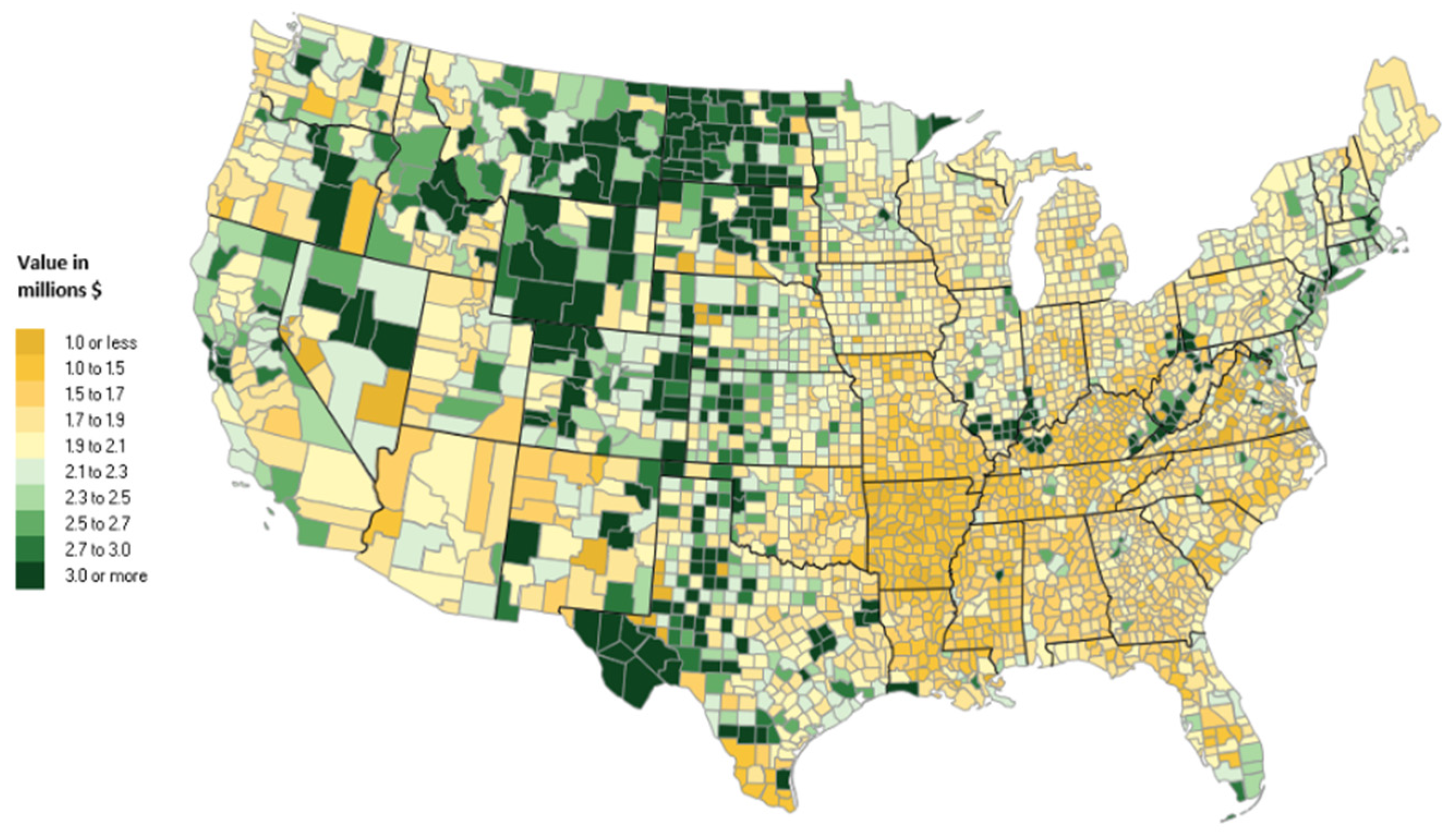
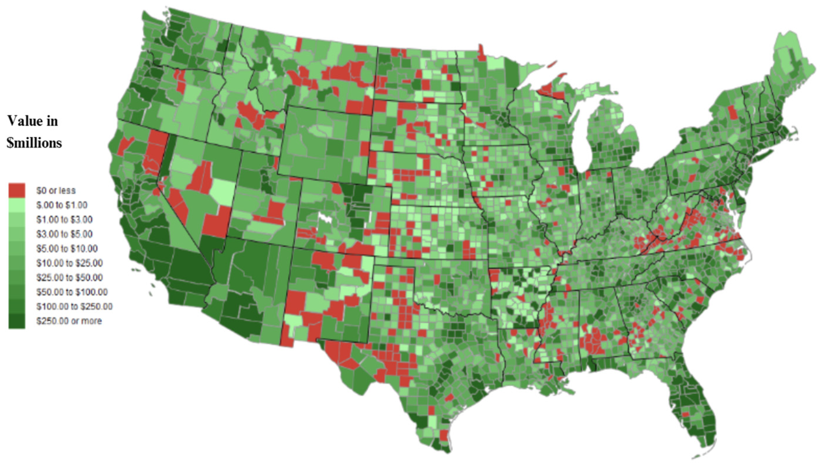
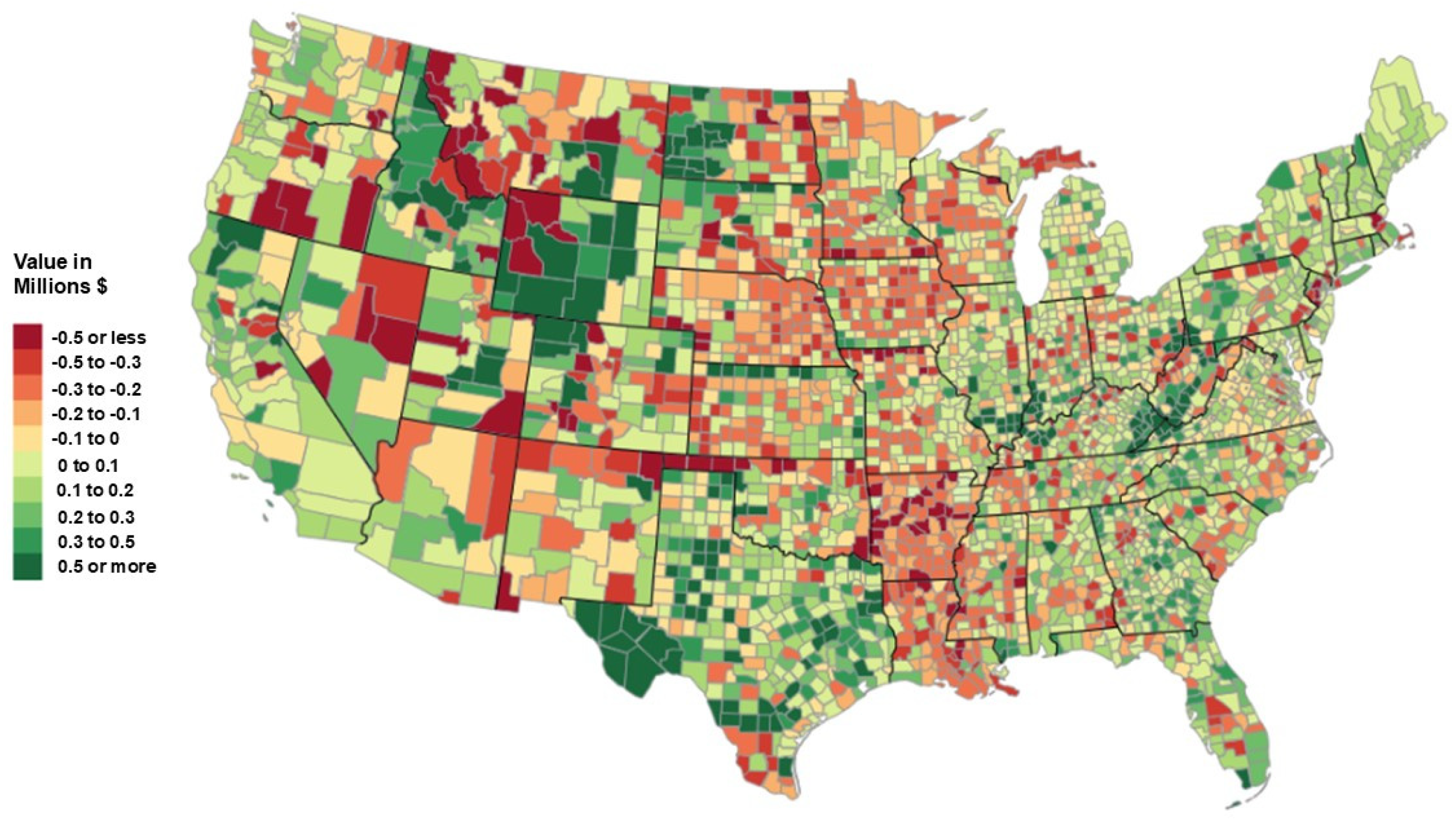
Our empirical findings are reported in Figure 1, Figure 2 and Figure 3. The figures are helpful in communicating the approximate magnitude of IW per capita in 2017, which varies substantially across the nation (Figure 1), and the substantial impact on measured IW per capita when calculated using the methods of Jones [21] (Figure 2) and those of Arrow et al. [5] (Figure 3). For a full list of the 3108 counties and their relative change in per capita IW between 2010 and 2017, please see the Supplementary Materials.

In Figure 1, per capita IW in 2017 exhibits a tendency for relatively low-population counties in Appalachia, the great plains, and the mountain west to rank highly in IW per capita, presumably driven by high NC per capita. However, as we see in Figure 2, not all of these counties were WS from 2010 to 2017: that is, high levels of NC/capita in the closing year were not necessarily conducive to WS status. High-NC counties may be exposed to declines in NC, losing key environmental services, such as tree canopy cover.

Figure 3 displays the change in IW per capita from 2010 to 2017, calculated using the Arrow 2010 framework. IW includes the value of NC through oil, coal, natural gas, cropland, pasture, timber, non-timber forest benefits, and carbon damages. PC is proxied as the county’s net asset position through GDP. Productivity HC is calculated using a rate of return of 8.5% per year of education. The value of health HC is calculated as the expected discounted years of life remaining multiplied by the value of an additional year of life (assumed independent of age) of USD 6.3 million. The Arrow [5] methods assessed 5 percent of US counties as not WS.

Our framework and improved data [21] yielded very different results. Thirty-two states were WS from 2010 to 2017, and eighteen were not WS. Of national residents, 75% lived in the 32 WS states (i.e., a mean of 7.63 million residents per state), while 25% lived in the not-WS states (a mean of 4.51 million residents per state). There was one notable cluster of eight not-WS states in the great plains and the mountain states: Minnesota, North and South Dakota, Montana, Wyoming, Nebraska, Colorado, and New Mexico. This cluster includes several of the high-IW per capita counties identified in Figure 1. The remaining ten not-WS states were scattered. Further research may reveal attributes that are common among them.

Further, 61% of US counties were WS, and these counties accounted for 73% of the US population, whereas 39% of counties were not WS, accounting for 27% of the US population. Clearly, WS counties support more than their numerical share of the national population, and not-WS counties support less than their numerical share of the population. It was common for WS states to have some not-WS counties and for not-WS states to have some WS counties (lists of these counties, i.e., not-WS counties in WS states and WS counties in not-WS states are provided as Supplementary Materials). Of all the counties in WS states, 37% were not WS, accounting for 16% of these states’ population. This implies that not-WS counties in WS states tended to be rural and with small populations, suggesting large and perhaps growing disparities between urban and rural economies. On the other hand, 27% of counties in not-WS states were WS, and these WS counties accounted for 56% of their states’ population. Clearly, WS counties play a major economic role in not-WS states. Just over half the people in not-WS states live in WS counties, which themselves comprise only about a quarter of all the counties in these states; that is, WS areas in not-WS states are mostly confined to urban areas, while not-WS conditions prevail in many of the outlying counties. It seems that the political consequences of these disparities are revealed in the legislatures of more than a few states.

Sixty-five percent of all counties are rural, and rural counties were under-represented (58%) among WS counties and over-represented (73%) among not-WS counties. This suggests a tendency to weakness in rural economies but, nevertheless, (i) 58% of WS counties nationwide were rural, suggesting that there are many success stories among rural counties that are sustainable, and (ii) 27% of not-WS counties were urban, demonstrating that urban counties are far from immune to sustainability challenges.

7. Discussion and Conclusions

We offer conceptual and empirical conclusions. Conceptually, we confirmed that change in IW per capita is the correct measure for WS assessment, provided the effects of population agglomeration are properly captured. That is, population matters to the sustainability of regions, but the WS criterion focuses on how well the population is living and saving for the future, rather than how many people there are. However, we concede explicitly that (i) weak sustainability is not an optimization framework and (ii) that we have not resolved the longstanding ethical questions implicit in trade-offs between total IW and IW per capita.

We highlighted a seldom-recognized problem in WS assessment that is left unresolved by the WS per capita criterion. It is customary in addressing intergenerational equity to posit generational persons (unitary decision-makers for each generation, which renders irrelevant the distinction between mean and median welfare or wealth) and, assuming monotone IW trajectories, requires non-diminishing welfare for each generation. However, each generation, in its turn, will be attentive to intragenerational equity criteria. Typically, (i) costs exceed benefits in the early stages of sustainability projects, and (ii) with right-skewed wealth and income, plausible equity criteria are bounded by the maximedian and the maximin. So, the discussion surrounding the typical project proposed by the present generation will tend to be framed in terms of costs and intragenerational equity criteria. Real people make these decisions about meeting their generation’s commitment to the welfare of future generations. Given that the average person enjoys substantially less than the mean IW per capita, debates about sustainability projects and programs are likely to focus on the median cost, i.e., the average person’s contribution to generational self-sacrifice. For most people, the ideal distribution lies in the range bounded by maximedian and maximin.

We utilized the framework of Jones [21] to assess the WS of states and counties in the US and compared our empirical results with those obtained with the Arrow et al. [5] framework. The difference is striking—we concluded that 39% of US counties were not WS from 2010 to 2017, whereas the Arrow methods found just 5% not WS. The largest contributor to the difference in results of the Jones and Arrow frameworks is Jones’ accounting for migration and regional differences in productivity and health quality. These results underscore the role of health quality as an important input for productivity and that cross-county migration is selective, favoring the young and highly skilled.

Our WS assessments at state and county levels in the US confirmed some prior expectations. There was an urban tilt toward WS status, showing most prominently in the finding that WS urban counties in not-WS states supported a majority of these states’ populations. Nevertheless, 58% of WS counties were rural, suggesting that there are many avenues for success among rural counties.

In theory and practice, our WS assessment at the county-level was limited by imperfections in relevant theory, methods, and data availability. The data-driven parts of our research were all limited by the data we were able to obtain and use. There were some omissions of potentially large assets, including the whole social and governance capital category, and mobile produced capital. The natural capital category suffered from restricted data resources, in that not all meaningful differences in resource quality were reflected in the data.

Looking forward, we offer several suggestions for a research agenda.

Is WS a preferred, e.g., more cost-effective, measure of sustainability compared to the alternatives? WS offers a more comprehensive assessment than, e.g., a battery of sustainability indicators but, due to its substantial data requirements, at potentially higher cost.

The more surprising results of our WS assessment—e.g., the relatively large number of rural counties among those that were WS, and the substantial role that WS cities played in the economies of not-WS states—suggested a large and potentially fruitful research agenda to dig a little deeper beneath the surface and identify the characteristics favorable for weak sustainability at the regional scale.

Does the WS status of states and counties based on the 2010–2017 assessment predict WS status going forward? A modest degree of reshuffling is to be expected, but we hypothesize that the trajectory of WS status from 2010 to 2017 is a good predictor of the WS status going forward and, as these more recent data become available, we foresee a rich research agenda to identify the conditions that enable or condemn, as the case may be, some counties to reverse their WS status.

How do the regional science and WS research agendas compare? Can they converge into a sustainable regional growth agenda or are there persistent methodological differences in the two approaches? Are there additional adjustments to IW per capita that are necessary, or even possible, to more fully capture the external scale (dis)economies of population size and density? Regardless of whether their agendas converge or not, what are the additional insights that can be gleaned by applying a WS framework to longstanding regional science questions of regional growth, competitiveness, and prosperity?