Dynamic Identification of Relative Poverty Among Chinese Households Using the Multiway Mahalanobis–Taguchi System: A Sustainable Livelihoods Perspective

Abstract

To promote global sustainable development, this paper focuses on the identification of relative poverty. On the one hand, based on the sustainable livelihoods framework, a multi-dimensional relative poverty identification index system is constructed, covering six dimensions—human capital, financial capital, natural capital, physical capital, social capital, and livelihood environment—with a total of 18 indexes. On the other hand, addressing the limitations of traditional relative poverty identification methods in handling dynamic three-dimensional data, the multiway Mahalanobis–Taguchi system (MMTS) is proposed to identify dynamic relative poverty. This method first unfolds dynamic three-dimensional data into two-dimensional data along the sample direction through multiway statistical analysis techniques, then constructs multiway Mahalanobis distances to measure sample differences, and finally uses a Taguchi orthogonal experimental design for dimensionality reduction and noise reduction to optimize the model. Experiments using tracking survey data from 2020 to 2024 in three poverty-stricken counties in China’s Dabie Mountain area show that MMTS performs better than the Two-Way Fixed Effects (Two-way FE) model and Dynamic LSTM. MMTS shows a higher specificity, stronger noise resistance, smaller result fluctuations, better G-means performance, and a better balance between sensitivity and specificity. This proves its scientific validity and practical applicability.

1. Introduction

In 2020, the Chinese government officially reported that its targeted poverty alleviation strategy had lifted 98.99 million rural residents out of absolute poverty [1]. This achievement marks the realization of China’s goal of eliminating absolute poverty. However, the eradication of absolute poverty does not signify the end of China’s poverty reduction efforts. In the subsequent stage of development, addressing relative poverty—rooted in structural inequalities and social exclusion—has become a core task for pursuing social equity goals [2,3]. Effective policy design relies on the accurate identification of relative poverty, yet this concept remains contested globally in both its definition and measurement [4]. Early studies often used a single income dimension to identify relative poverty [5,6]. While such approaches are operationally straightforward, they are increasingly criticized for failing to reflect the complexity, multidimensionality, and dynamic nature of relative poverty [7]. These approaches typically overlook non-economic deprivations such as unequal access to education, limited healthcare availability, and restricted social participation [2,3,4]. To address these issues, scholars have proposed multi-dimensional approaches to identify relative poverty [8,9]. For instance, Wang argues that relying solely on income indexes is insufficient to align with China’s broader socioeconomic development objectives [10]. She proposes a framework integrating economic, social, and ecological dimensions to better reflect material deprivation, social hardship, and environmental constraints. Based on this framework, Wang et al. [11] developed a hybrid model combining income and non-income indexes to improve identification accuracy.

Existing studies have also attempted to enrich the dimensions of relative poverty from perspectives of inequality and social exclusion. For example, Wan et al. [12] explored how disparities in access to employment, education, and training contribute to persistent poverty from the perspective of income inequality. Silver [3] emphasized that social exclusion involves not only economic scarcity but also a lack of participation in social interactions, decision-making, and public services. The absence of such participation and recognition exacerbates the condition of relative poverty. Parolin et al. [13] highlighted that the intergenerational transmission of relative poverty is not limited to economic factors but also includes the inheritance of social capital. Educational disadvantages make it hard for children in relatively poor households to bridge class gaps and may lead to long-term disadvantages.

Despite these advances, key theoretical and methodological limitations remain. Most existing models rely on static thresholds, failing to account for the dynamic evolution of household livelihoods under external shocks such as policy changes or natural disasters [14]. Moreover, while social exclusion theory highlights institutional barriers, it lacks a robust framework for quantifying the interactions between human capital (e.g., education), financial capital (e.g., income stability), and social capital (e.g., networks and trust)—all of which are critical for identifying relative poverty [15,16].

Regarding the identification methods of relative poverty, with the rapid development and widespread application of big data technology, data-driven approaches have increasingly become a research hotspot. These methods utilize rich datasets and advanced algorithms to uncover the internal laws of relative poverty. However, in contrast, the identification of relative poverty places more emphasis on an individual’s economic status relative to the social average in the socioeconomic structure, highlighting the inequality perceived by individuals and the resulting sense of relative deprivation. Therefore, how to accurately and effectively identify these two types of samples— the “reference group” and the “relatively impoverished group”—has become a key focus in current research on relative poverty identification methods. The current research follows three technical paths: (1) Statistical Inference: Models like linear regression and structural equation models analyze poverty mechanisms via variable relationships. For example, Ravallion’s poverty regression model reveals income–poverty dynamics [17]. Cluster analysis (e.g., k-means) and causal inference (e.g., DID models) address heterogeneity and policy effects [18,19]. (2) Machine Learning: Algorithms like decision trees and SVMs improve classification via feature engineering. Maruejols et al. used Random Forest to identify low capital income as a key poverty indicator in rural China [20]. Ensemble methods (e.g., XGBoost) and deep learning (e.g., LSTM) enhance the prediction accuracy for dynamic poverty patterns [21,22]. (3) Deep Learning: CNNs visualize poverty geography via satellite imagery, while RNNs/LSTMs process time-series data for trend forecasting [23,24].

However, these methods face critical limitations: (1) Time-series models (e.g., ARIMA) require strict stationarity and fail to capture multidimensional interactions. (2) Panel data models (e.g., fixed-effects regression) lose cross-dimensional information during variable aggregation. (3) Machine learning (e.g., LSTM) lacks interpretability, hindering a causal analysis of poverty drivers. To tackle the above issues, this paper proposes a multi-dimensional relative poverty identification index system based on the sustainable livelihoods framework (SLF) [25] and develops MMTS to improve dynamic three-dimensional data processing to identify dynamic relative poverty.

The structure of this paper is organized as follows: In Section 2, an index system for identifying relative poverty is constructed from the perspective of sustainable livelihoods. In Section 3, MMTS is established using multiway statistical analysis techniques and the Mahalanobis–Taguchi system (MTS). In Section 4, we validate the performance of the proposed method for the dynamic identification of relative poverty using real-world case data. Section 5 presents the conclusions and future research directions.

2. Construction of the Index System for Identifying Relative Poverty from the Perspective of Sustainable Livelihoods

SLF is a conceptual and analytical tool that helps understand how individuals, households, and communities build and manage their livelihoods when facing environmental, economic, and social challenges. It emphasizes the dynamic interactions among different livelihood components and their long-term sustainability. Developed in the 1990s by the UK’s Department for International Development (DFID), it has since been widely adopted and adapted by various organizations and researchers around the world to address issues related to sustainable development. The core components of SLF consist of four key elements: livelihood assets, vulnerability context, livelihood strategies, and livelihood outcomes. Livelihood assets encompass human capital (individual skills and knowledge), social capital (social networks), financial capital (savings and credit), physical capital (infrastructure), and natural capital (natural resources), serving as the foundation for maintaining livelihoods. The vulnerability context includes external risk factors such as economic fluctuations and climate change. Livelihood strategies refer to the activities and choices made by individuals or households to achieve goals like the generation of income and food security. Livelihood outcomes are the expected results of these strategies, such as a reduction in poverty and the utilization of sustainable resources.

Unlike static approaches (e.g., MPI’s fixed thresholds) or single-dimensional theories (e.g., social exclusion), SLF emphasizes the following: (1) Capital Interactions: A low education level (human capital) restricts income growth (financial capital), creating self-reinforcing poverty cycles. (2) Dynamic Adaptation: Households adjust livelihood strategies in response to shocks (e.g., rural families diversifying into non-farm work after agricultural policy reforms) [26]. In the Chinese context, SLF aligns with post-2020 poverty governance goals of “common prosperity” through multidimensional interventions. For instance: (1) Policy Coherence: The framework’s health capital indexes (e.g., the prevalence of chronic disease) directly support China’s “Health Poverty Alleviation” initiatives, while physical capital metrics (e.g., digital infrastructure coverage) resonate with the “Digital Village” strategy. (2) Regional Adaptability: Unlike MPI’s uniform thresholds, SLF allows weighted indexes tailored to local contexts—prioritizing natural capital (e.g., arable land quality) in agricultural regions and social capital (e.g., community organization participation) in migrant-dense areas. As an integrated tool, SLF systematically evaluates household livelihoods by analyzing interlinked capital dimensions and their temporal evolution. This not only enhances the scientific accuracy of relative poverty’s identification but also provides a forward-looking framework for designing context-specific poverty reduction policies, such as targeted skill training in urban–rural migrant communities or ecological compensation mechanisms in western mountainous areas.

Therefore, this paper constructs a set of identification index systems for relative poverty based on the SLF, as shown in

Table 1. Identification indexes and screening criteria for relative poverty from the perspective of sustainable livelihoods.

Dimension	Index	Screening Criteria
Human Capital	Average years of education for adults (X1)	Reflect the long-term impact of the knowledge reserve on income-earning ability and block the intergenerational transmission of poverty.
	Health status of household members (X2)	Measure the direct weakening of diseases in terms of labor capacity, echoing the health–poverty alleviation policy.
	School enrollment rate for children of school age (X3)	Monitor educational equity and prevent the intergenerational transmission of capability poverty.
	Participation rate in vocational skill training (X4)	Meet the requirements of industrial upgrading and improve the adaptability to non-agricultural employment.
Financial Capital	Annual per capita household income (X5)	Serve as a core explicit index for accessing economic resources.
	Family savings/debt ratio (X6)	Warn of debt risks and identify groups with weak economic resilience.
Natural Capital	Area and quality of cultivated land (X7)	Reflect the livelihood foundation of agriculture-based households and align with policies such as returning farmland to forests.
	Degree of dependence on natural resources (X8)	Monitor the pressure on alternative livelihoods in ecologically fragile areas caused by environmental policies (e.g., logging bans).
Physical Capital	Compliance rate of housing conditions (X9)	Housing is the core of basic living security, directly affecting health and safety. Dilapidated or simple-structured houses are vulnerable to natural disasters, exacerbating vulnerability to poverty.
	Accessibility of safe drinking water (X10)	Access to safe drinking water is fundamental to health and productivity. The lack of drinking water increases the risk of diseases and the cost of living.
	Coverage rate of sanitary facilities (X11)	Poor sanitation facilities are prone to the transmission of disease, increasing the burden of medical expenses.
	Number of durable consumer goods (X12)	Household appliances and transportation tools reflect the convenience of life and the ability to resist risks.
	Transportation convenience (X13)	Transportation conditions affect access to employment opportunities, as well as the accessibility of education and healthcare resources, limiting social participation.
Social Capital	Strength of social network support (X14)	Social networks serve as an informal safeguard for families to cope with sudden risks (e.g., illness, unemployment), reflecting the mutual aid capacity of social relationships.
	Degree of participation in community organizations (X15)	The ability to undertake collective action enhances opportunities for the acquisition of resources and policy benefits through organizations such as cooperatives and mutual aid associations.
Livelihood Environment	Degree of infrastructure completion (X16)	Infrastructure is the foundation of economic development, directly affecting production efficiency and market access.
	Accessibility of public services (X17)	The accessibility of public services such as education, medical care, and markets reduces the inequality of opportunities and lowers living costs.
	Degree of exposure to natural disaster risks (X18)	Environmental vulnerability directly threatens the stability of livelihoods, especially for household’s dependent on agriculture and natural resources.

.

This index system comprehensively covers various types of livelihood capital, such as human, financial, natural, physical, and social capital. At the same time, it takes into account the elements of the livelihood environment where rural households are located. The principles followed in index screening are as follows: (1) Multidimensional coverage. We break through the limitations of the single income dimension and reveal the complexity of poverty through the interaction of the five types of capital. (2) Dynamic early warning. The debt ratio is incorporated to identify the potential risks of blocked capital transformation (for example, high debt weakens the liquidity of financial capital). Additionally, indexes such as natural disasters are introduced to warn of the vulnerability to returning to poverty caused by environmental shocks. (3) Policy coherence. The indexes directly correspond to national strategies such as “Rural Revitalization” and “Common Prosperity” (for example, vocational skill training is aligned with the alleviation of employment poverty). (4) Compatibility with regional differences. By adjusting the priorities and weights of indexes to reflect local conditions, the framework fully accounts for regional differences in poverty. For example, cultivated land’s quality is assigned a greater weight in the mountainous western regions, while vocational skills training rates are prioritized in the urbanized eastern areas. This region-specific adjustment balances urban–rural and east–west differences, while avoiding the misclassifications that a uniform, “one-size-fits-all” approach would inevitably produce. (5) Data viability. The framework gives priority to quantifiable and easily trackable indexes sourced from registered poverty records and rural census data, enabling grassroots officials to implement them.

3. Construction of the Multiway Mahalanobis–Taguchi System

3.1. Proposal of the Multiway Mahalanobis–Taguchi System

The Mahalanobis–Taguchi system (MTS) is a pattern recognition method for imbalanced data proposed by Dr. Genichi Taguchi, a renowned Japanese quality engineer, in the early 1990s [27,28]. This method constructs a recognition model by integrating three core tools: Mahalanobis distance (MD), orthogonal array (OA), and signal-to-noise ratio (SNR). Specifically, it first uses the Mahalanobis distance to measure the deviation of samples from a reference benchmark (as shown in Figure 1), then establishes a robust feature selection mechanism through a Taguchi orthogonal experimental design [29], and finally it combines the signal-to-noise ratio to achieve the screening of key features.

Compared with traditional pattern recognition techniques, MTS has the following advantages [27]. First, it overcomes the restrictive assumption of data’s normal distribution in traditional methods. By integrating the system optimization theory from Taguchi quality engineering, MTS significantly enhances computational efficiency while maintaining the simplicity of the method. Second, it achieves identification through the establishment of a unified reference benchmark, so it has a simple principle and is easy to operate. However, the conventional MTS relies on a static multidimensional data analysis model, which is not suitable for the dynamic nature of relative poverty. According to SLF, the vulnerability context, livelihood assets, and livelihood strategies of impoverished groups undergo a multi-dimensional evolution over time (e.g., the prolonged impacts of economic fluctuations, policy adjustments, or natural disasters), which requires dynamic three-dimensional data (samples × time × variables) to reflect the continuous change trends of poverty status. However, the traditional MTS relies on static Mahalanobis distances and cannot integrate time-series information well. This makes it unable to fully describe the dynamic aspects of poverty (e.g., poverty’s duration and fluctuation amplitude).

To address this limitation, this paper proposes an improved version of the traditional MTS: the multiway Mahalanobis–Taguchi System (MMTS). On one hand, MMTS utilizes multiway statistical analysis techniques [30] to establish multiway Mahalanobis distances to process dynamic three-dimensional data, dynamically tracking the correlations of poverty characteristics across different time points. On the other hand, the proposed model uses a Taguchi orthogonal experimental design to reduce data dimensions and remove noise, which improves the data quality while keeping important time-series information. MMTS retains the advantages of the traditional MTS in terms of benchmark construction and computational efficiency, while aligning closely with SLF’s principles of dynamic adaptability and multidimensional integration. As a result, it provides a technically reasonable and practical way to identify dynamic poverty.

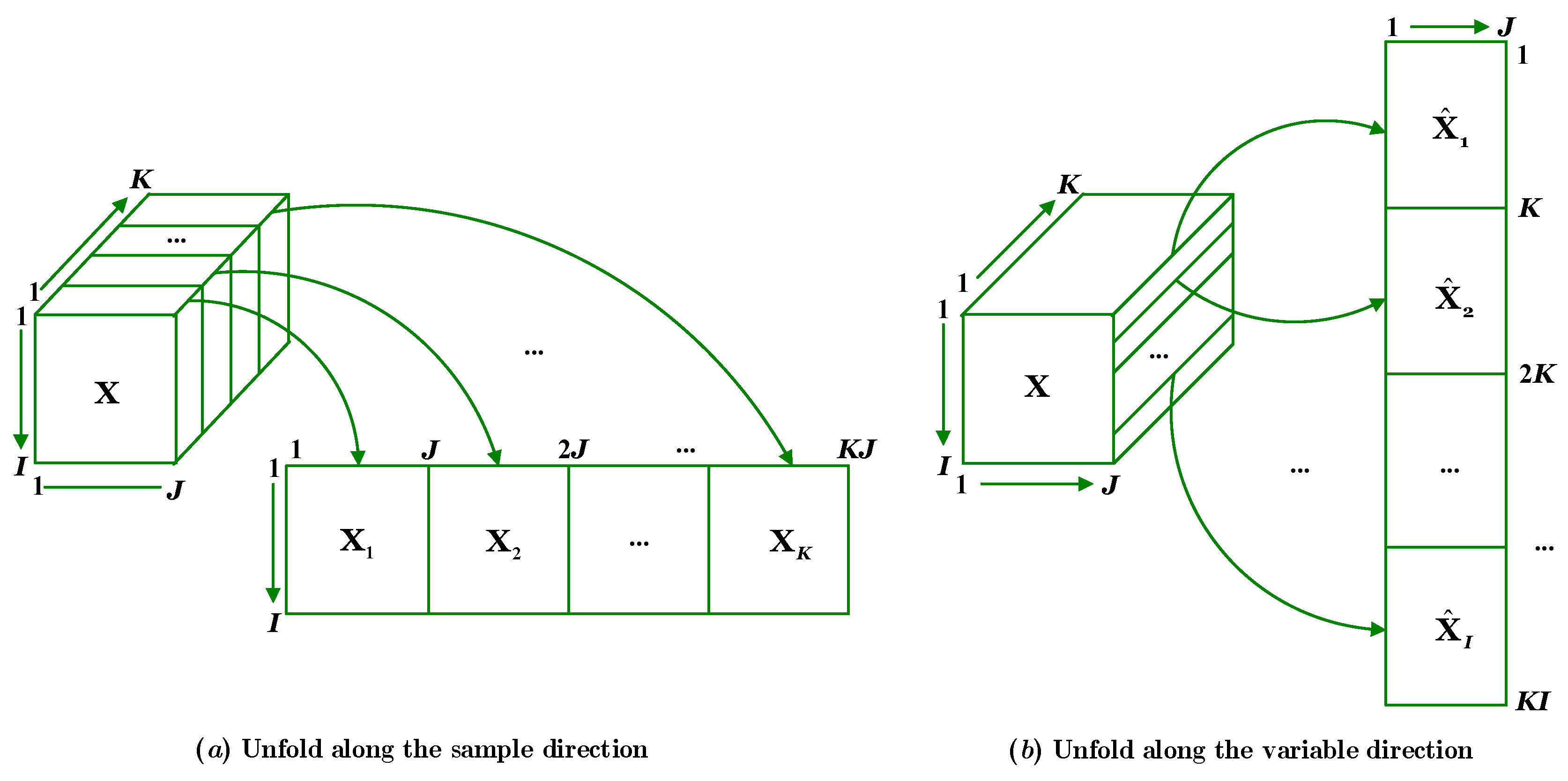
3.2. Multiway Mahalanobis Distance

Multiway statistical analysis, also known as multi-dimensional data analysis or multi-modal modeling, is a core method for handling high-dimensional and complex data structures. It is particularly suitable for datasets with spatiotemporal correlations and multi-source heterogeneity [31].

The key to constructing the multiway Mahalanobis distance is that multiway statistical analysis techniques are applied to unfold a dynamic three-dimensional matrix (Samples I × Time K × Variables J) into a static two-dimensional matrix. Six ways are applied to unfold a dynamic three-dimensional matrix into a static two-dimensional matrix, but only two of them have statistical significance. One is to unfold it in the sample direction. In this unfolding method, the data in the Time K and Variables J directions are combined to form a two-dimensional matrix, as shown in Figure 2a. The other is to unfold it in the variable direction. In this unfolding method, the data in the Samples I and Time K directions are combined to form a two-dimensional matrix, as shown in Figure 2b.

The row vectors of the two-dimensional matrix unfolded in the sample direction can integrate the trajectories of all the variables of a single sample across all time points. It can effectively reflect the changing trends in relative poverty at different time points. Therefore, this paper unfolds the dynamic three-dimensional matrix in the sample direction. Based on this, the MMD is derived. The specific derivation process is as follows:

Let $\underset{\_}{\mathbf{X}}(I\times J\times K)$ be a dynamic three-dimensional matrix, where $I$ represents the number of samples, $J$ represents the number of characteristic variables, and $K$ represents the statistical time points. In the following, the three-dimensional matrix $\underset{\_}{\mathbf{X}}(I\times J\times K)$ is processed by retaining the sample dimension and merging the time and variable dimensions to obtain a two-dimensional matrix.

$$\mathbf{X}\in {ℝ}^{I\times (K·J)}$$

(1)

where the i-th sample in $\mathbf{X}$ is denoted as ${\mathit{x}}_i\in {ℝ}^{K·J}$, $i=1,2,\cdots ,I$.

Then, the MMD of the sample ${\mathit{x}}_i\in {ℝ}^{K·J}$ is defined as

$${\mathrm{MMD}}_i^2={({\mathit{x}}_i-\overline{\mathit{x}})}^{\mathrm{T}}{\mathbf{S}}^{-1}({\mathit{x}}_i-\overline{\mathit{x}})$$

(2)

where $\overline{\mathit{x}}\in {ℝ}^{K·J}$ is the sample mean vector, and the calculation formula is as follows:

$$\overline{\mathit{x}}={\displaystyle \frac{1}{I}}{\displaystyle \sum _{i=1}^I{\mathit{x}}_i}$$

(3)

$\mathbf{S}\in {ℝ}^{(K·J)\times (K·J)}$ is the covariance matrix, and the calculation formula is as follows:

$$\mathbf{S}={\displaystyle \frac{1}{I-1}}{\displaystyle \sum _{i=1}^I({\mathit{x}}_i-\overline{\mathit{x}})}{({\mathit{x}}_i-\overline{\mathit{x}})}^{\mathrm{T}}$$

(4)

Proposition 1. 

For $I$ independent and identically distributed normal samples, we have

$$\mathbb{E}({\mathrm{MMD}}_i^2)=K·J$$

(5)

Proof. 

First, centralize the data. Let ${\tilde{\mathit{x}}}_i={\mathit{x}}_i-\overline{\mathit{x}}$; the covariance matrix is as

$$\mathbf{S}={\displaystyle \frac{1}{I-1}}{\displaystyle \sum _{i=1}^I{\tilde{\mathit{x}}}_i}{\tilde{\mathit{x}}}_i^{\mathrm{T}}$$

(6)

Then, decompose the covariance matrix as follows:

$$\mathbf{S}=\mathbf{Q}\mathbf{\Lambda }{\mathbf{Q}}^{\mathbf{T}}$$

(7)

where $\mathbf{Q}$ is an orthogonal matrix, and $\mathbf{\Lambda }=\mathrm{diag}({\mathsf{\lambda }}_1,{\mathsf{\lambda }}_2,\cdots ,{\mathsf{\lambda }}_{K·J})$ is a diagonal matrix of eigenvalues.

The expected value of MMD is calculated as follows:

$$\mathbb{E}({\mathrm{MMD}}_i^2)=\mathbb{E}\left[{({\tilde{\mathit{x}}}_i)}^{\mathrm{T}}{\mathbf{S}}^{-1}{\tilde{\mathit{x}}}_i\right]$$

(8)

According to the properties of the trace, we have

$$\mathbb{E}\left[{\tilde{\mathit{x}}}_i^{\mathrm{T}}{\mathbf{S}}^{-1}{\tilde{\mathit{x}}}_i\right]=\mathrm{tr}\left(\mathbb{E}\left[{\tilde{\mathit{x}}}_i{\tilde{\mathit{x}}}_i^{\mathrm{T}}{\mathbf{S}}^{-1}\right]\right)$$

(9)

Since $\mathbb{E}\left[{\tilde{\mathit{x}}}_i{\tilde{\mathit{x}}}_i^{\mathrm{T}}\right]=\mathbf{S}$, we have

$$\mathbb{E}({\mathrm{MMD}}_i^2)=\mathrm{tr}\left({\mathsf{I}}_{K·J}\right)=K·J$$

(10)

where $\mathbf{I}$ is the identity matrix. □

To make the mean value of the MMDs of the normal samples approach 1, Equation (2) is rewritten in the following form:

$${\mathrm{MMD}}_i^2={\displaystyle \frac{1}{K·J}}{({\mathit{x}}_i-\overline{\mathit{x}})}^{\mathrm{T}}{\mathbf{S}}^{-1}({\mathit{x}}_i-\overline{\mathit{x}}), i=1,2,\cdots ,I$$

(11)

where $K$ represents the time points for statistical analysis, $J$ denotes the number of feature variables, ${\mathit{x}}_i\in {ℝ}^{K·J}$ is the vector of the unfolded sample, $\overline{\mathit{x}}\in {ℝ}^{K·J}$ is the mean vector of the unfolded normal samples, and $\mathbf{S}\in {ℝ}^{(K·J)\times (K·J)}$ is the covariance matrix of the unfolded normal samples.

3.3. Taguchi Orthogonal Experimental Design

MTS employs the Taguchi orthogonal experimental design proposed by Dr. Genichi Taguchi for feature selection to improve the identification accuracy. The Taguchi orthogonal experimental design aims to study the influence of multiple factors on the experimental results with the minimum number of experiments and determine the optimal conditions. In MTS, a two-level orthogonal array (denoted as $L_N(2^k)$, where N is the number of experiments, k is the number of factors, and 2 is the number of levels) is used to construct the combination scheme of feature subsets. Suppose there are six feature variables. An $L_8\left(2^7\right)$ orthogonal array can be selected, and these six feature variables are randomly assigned to any six columns of the orthogonal array. Here, “1” indicates that the feature variable participates in the construction of the reference benchmark, while “2” means it is excluded. Each row of the orthogonal array corresponds to a feature combination scheme, to generate eight reference benchmarks with different dimensions, as shown in

Table 2. Taguchi orthogonal experiment.

Experiment	$X_1$	$X_2$	$X_3$	$X_4$	$X_5$	$X_6$		The MMDs of Abnormal Samples				$\mathrm{SNR}$
	1	2	3	4	5	6	7	1	2	…	$Q$
1	1	1	1	1	1	1	1	${\widehat{\mathrm{MMD}}}_{11}^2$	${\widehat{\mathrm{MMD}}}_{12}^2$	…	${\widehat{\mathrm{MMD}}}_{1Q}^2$	${\mathrm{SNR}}_1$
2	1	1	1	2	2	2	2	${\widehat{\mathrm{MMD}}}_{21}^2$	${\widehat{\mathrm{MMD}}}_{22}^2$	…	${\widehat{\mathrm{MMD}}}_{2Q}^2$	${\mathrm{SNR}}_2$
3	1	2	2	1	1	2	2	${\widehat{\mathrm{MMD}}}_{31}^2$	${\widehat{\mathrm{MMD}}}_{32}^2$	…	${\widehat{\mathrm{MMD}}}_{3Q}^2$	${\mathrm{SNR}}_3$
4	1	2	2	2	2	1	1	${\widehat{\mathrm{MMD}}}_{41}^2$	${\widehat{\mathrm{MMD}}}_{42}^2$	…	${\widehat{\mathrm{MMD}}}_{4Q}^2$	${\mathrm{SNR}}_4$
5	2	1	2	1	2	1	2	${\widehat{\mathrm{MMD}}}_{51}^2$	${\widehat{\mathrm{MMD}}}_{52}^2$	…	${\widehat{\mathrm{MMD}}}_{5Q}^2$	${\mathrm{SNR}}_5$
6	2	1	2	2	1	2	1	${\widehat{\mathrm{MMD}}}_{61}^2$	${\widehat{\mathrm{MMD}}}_{62}^2$	…	${\widehat{\mathrm{MMD}}}_{6Q}^2$	${\mathrm{SNR}}_6$
7	2	2	1	1	2	2	1	${\widehat{\mathrm{MMD}}}_{71}^2$	${\widehat{\mathrm{MMD}}}_{72}^2$	…	${\widehat{\mathrm{MMD}}}_{7Q}^2$	${\mathrm{SNR}}_7$
8	2	2	1	2	1	1	2	${\widehat{\mathrm{MMD}}}_{81}^2$	${\widehat{\mathrm{MMD}}}_{82}^2$	…	${\widehat{\mathrm{MMD}}}_{8Q}^2$	${\mathrm{SNR}}_8$

.

Then, the following formula is used to calculate the MMDs of abnormal samples under each reference benchmark, as follows:

$${\widehat{\mathrm{MMD}}}_q^2={\displaystyle \frac{1}{K·J}}{({\mathit{x}}_q^{\prime }-\overline{\mathit{x}})}^{\mathrm{T}}{\mathbf{S}}^{-1}({\mathit{x}}_q^{\prime }-\overline{\mathit{x}}), q=1,2,\cdots ,Q$$

(12)

where $K$ represents the time point for statistical analysis, $J$ denotes the dimensionality of the reference benchmark, $Q$ indicates the number of abnormal samples, ${\mathit{x}}_q^{\prime }\in {ℝ}^{K·J}$ is the vector of the q-th abnormal sample in the two-dimensional sample matrix obtained by unfolding the three-dimensional sample matrix, and $\overline{\mathit{x}}\in {ℝ}^{K·J}$ and $\mathbf{S}\in {ℝ}^{(K·J)\times (K·J)}$ are respectively the mean vector and the covariance matrix of the two-dimensional normal sample matrix obtained by unfolding the three-dimensional normal sample matrix.

Next, the effectiveness in identification of each feature combination is quantified by calculating the SNR. The calculation formula is as follows:

$${\mathrm{SNR}}_p=-10\log \left({\displaystyle \frac{1}{Q}}{\displaystyle \sum _{q=1}^{\mathrm{Q}}\frac{1}{{\widehat{\mathrm{MMD}}}_{pq}^2}}\right), p=1,2,\cdots ,N$$

(13)

where ${\mathrm{SNR}}_p$ is the SNR of the p-th experiment, and ${\widehat{\mathrm{MMD}}}_{pq}^2$ is the MMD of the q-th abnormal sample in the p-th experiment.

Finally, the information gain of each variable is calculated, and the key variables that make significant contributions to the classification are selected. The calculation formula is as follows:

$${\mathrm{Gain}}_j={\overline{\mathrm{SNR}}}_j^{+}-{\overline{\mathrm{SNR}}}_j^{-}, j=1,2,\cdots ,J$$

(14)

where ${\overline{\mathrm{SNR}}}_j^{+}$ represents the average SNR of all the experiments in which the feature variable $X_j$ is involved; ${\overline{\mathrm{SNR}}}_j^{-}$ represents the average SNR of all the experiments in which the feature variable $X_j$ is not involved. If ${\mathrm{Gain}}_j>0$, the feature variable $X_j$ is retained; otherwise, the feature variable is deleted.

3.4. Calculation Steps

In summary, the specific calculation steps of MMTS are outlined below:

Step 1: Multi-way data unfolding.

Using multiway statistical analysis techniques, the three-dimensional matrix is unfolded into a two-dimensional matrix along the sample direction.

Step 2: Construction of the reference benchmark.

A total of I normal samples are selected to calculate the MMD for each normal sample using Equation (11). These MMD values together constitute the reference benchmark. This benchmark is used as a standard to identify abnormal samples in the following steps.

Step 3: Validation of the reference benchmark.

A total of Q abnormal samples are selected, and their MMD values are computed using Equation (12). Then, the MMDs of the abnormal samples are compared with those of the normal samples. Typically, if the MMDs of the abnormal samples are significantly higher than those of the normal samples, it indicates that the constructed reference benchmark is effective.

Step 4: Optimization of the reference benchmark.

First, an appropriate two-level orthogonal array is selected based on the dimensionality of the sample variables. Then, according to the reference benchmark determined in each experiment, we use Equation (12) to calculate the MMDs of the abnormal samples. Finally, Equation (14) is applied to screen the feature variables.

Step 5: Threshold determination.

The optimized reference benchmark is employed to recalculate the MMDs of the normal samples and the abnormal samples. An appropriate threshold is then determined based on the calculation results.

4. Case Study Application

4.1. Data Source and Sampling Methods

The data for this study were obtained from three rounds of follow-up surveys conducted in 2020, 2022, and 2024 in the concentrated contiguous poverty-stricken areas of the Dabie Mountains, China. A stratified random sampling method was adopted. Three former nationally designated poverty-stricken counties (anonymized as Counties A, B, and C) were selected based on geographic poverty characteristics (mountainous terrain > 70%) and distinct poverty alleviation pathways (eco-compensation, rural tourism, and labor export). Five townships were randomly sampled from each county, followed by the random selection of three administrative villages from each township. Subsequently, within each administrative village, 10 to 15 households were randomly chosen. The initial baseline sample comprised 960 households, and after the follow-up surveys, an effective dataset of 895 households was established, with an attrition rate of 7.8%.

The questionnaire comprehensively covered all 18 indexes presented in Table 1. To guarantee data objectivity and analytical validity, each index was rigorously quantified and assigned values on a standardized 1-to-5 scale. This method precisely quantifies relevant information for the sample regions, as shown in

Table 3. Explanation and assignment of the indexes for identifying relative poverty.

Dimension	Index	Explanation and Assignment
Human Capital	Average years of education for adults (X1)	The average years of education of the main labor force in a household reflect the household’s capacity to generate income through knowledge and skills. A low level of education may lead to the intergenerational transmission of poverty. (more than 16 years = 5, 12–16 years = 4, 9–12 years = 3, 6–9 years = 2, less than 6 years = 1)
	Health status of household members (X2)	The proportion of household members suffering from chronic diseases or disabilities. The health level directly affects the labor capacity and the burden of medical expenditure. (%)
	School enrollment rate for children of school age (X3)	The actual enrollment rate of children aged 6 to 15 in the household, which measures the fairness of educational opportunities. A low enrollment rate may indicate a shortage of future human capital. (%)
	Participation rate in vocational skill training (X4)	The proportion of household members participating in vocational skill training reflects the household’s ability to improve employment opportunities through skill enhancement. (%)
Financial Capital	Annual per capita household income (X5)	The annual average value of the total household income divided by the number of household members directly reflects the ability to acquire economic resources and is a core measurement standard for poverty.
	Family savings/debt ratio (X6)	The proportion of household savings or liabilities to the annual income. A high debt ratio can indicate economic vulnerability and debt risks. (%)
Natural Capital	Area and quality of cultivated land (X7)	The area of arable land owned by a household and its soil fertility level represent the foundation of their livelihood for agriculture-dependent households; land scarcity may lead to poverty. (more than 5 mu with high fertility = 5, 3–5 mu with high fertility = 4, 1–3 mu with medium fertility = 3, less than 1 mu with low fertility = 2, no land or barren land = 1)
	Degree of dependence on natural resources (X8)	The proportion of household income depends on natural resources such as forestry and fisheries; over-reliance on natural resources makes households vulnerable to environmental changes. (%)
Physical Capital	Compliance rate of housing conditions (X9)	Housing structure (e.g., brick–concrete or reinforced concrete) and whether the per capita living area meets standards reflect the level of basic living security. (reinforced concrete/≥15 m2 = 5, brick–concrete/12–15 m2 = 4, brick–timber/8–12 m2 = 3, simple structure/5–8 m2 = 2, dilapidated house/per capita area < 5 m2 = 1)
	Accessibility of safe drinking water (X10)	Whether a household can consistently access drinking water that meets sanitary standards; the lack of safe drinking water poses health risks and increases living costs. (indoor direct supply = 5, walking < 30 min = 4, walking 30–60 min = 3, walking > 1 h to fetch water = 2, no stable water source = 1)
	Coverage rate of sanitary facilities (X11)	Whether a household has access to a private toilet (e.g., flush toilet); poor sanitation conditions may increase the risk of disease. (private flush toilet = 5, shared flush toilet = 4, simple dry toilet = 3, open-air toilet = 2, no toilet = 1)
	Number of durable consumer goods (X12)	The number of household appliances (e.g., refrigerator, washing machine) and means of transportation (e.g., electric vehicles, cars) reflects the level of convenience in life and resilience to risks. (≥7 items, including high-value assets such as cars = 5, 5–6 items = 4, 3–4 items = 3, 1–2 items = 2, 0 items = 1)
	Transportation convenience (X13)	The walking time from a household to the nearest public transportation stop, which affects access to employment opportunities and social participation. (≤5 min = 5, 5–15 min = 4, 15–30 min = 3, 30–60 min = 2, >60 min = 1)
Social Capital	Strength of social network support (X14)	Whether a household can receive financial or material assistance from relatives, friends, or the community in emergencies; social networks are a critical resource for risk management. (abundant and reliable support = 5, stable and basic support = 4, regular but partial support = 3, occasional and minimal support = 2, no support at all = 1)
	Degree of participation in community organizations (X15)	Whether household members participate in organizations such as cooperatives or mutual aid groups; the capacity for collective action influences access to resources and opportunities to benefit from policies. (active participation in ≥2 organizations = 5, regular participation in 1 organization = 4, occasional participation in activities = 3, past participation but has withdrawn = 2, no participation = 1)
Livelihood Environment	Degree of infrastructure completion (X16)	The level of infrastructure coverage in the community, including roads, electricity, and communication networks; underdeveloped infrastructure limits economic development opportunities. (fully paved roads, stable electricity, and high-speed internet = 5; access to electricity and internet with partially paved roads = 4; fully paved roads and stable electricity but no internet = 3; partially paved roads and unstable electricity = 2; no paved roads and frequent power outages = 1)
	Accessibility of public services (X17)	The distance or travel time from a household to the nearest school, hospital, and market; insufficient access to public services increases living costs and exacerbates inequality. (all services within ≤1 km = 5, all services within 1–3 km = 4, all services within 3–5 km = 3, some services within 5–10 km = 2, all services >10 km = 1)
	Degree of exposure to natural disaster risks (X18)	The frequency and extent of losses caused by natural disasters, such as floods and droughts, in the region over the past five years. Environmental vulnerability threatens livelihood stability. (no disaster records = 5, one minor disaster = 4, one disaster with 10–30% loss = 3, two disasters with >30% income loss = 2, ≥3 major disasters in the past five years = 1)

.

In terms of the determination of the two types of samples, namely the “relatively impoverished group” and the “reference group”, we use the subjective welfare assessment method proposed by Rojas [32]. In the questionnaire design stage, the item of the self-rated household socioeconomic status scale was introduced. The specific expression is, “What level do you think your current household’s economic and social situation is in this area?” This measurement tool adopts the form of a Likert five-point scale and uses a continuous scoring method from 1 to 5. Among them, 1 point corresponds to the semantic anchoring of “Extremely poor”, and 5 points correspond to the semantic anchoring of “Very affluent” [33]. In this study, the surveyed households that chose 1 point (“Extremely poor”) and 2 points (“Poor”) are defined as the “relatively impoverished group”, and this group exhibits significant poverty characteristics in both the subjective cognition and objective condition dimensions. On the other hand, the samples that chose 3 points (“Medium level”), 4 points (“Relatively affluent”), and 5 points (“Very affluent”) are classified into the “reference group”. Finally, an effective three-dimensional sample dataset consisting of 895 households was constructed, as shown in

Table 4. Three-dimensional sample dataset.

Poverty County	Reference Group	Relatively Impoverished Group	Total
A	355	80	435
B	140	83	223
C	135	102	237
Total	630	265	895

.

4.2. Evaluation Indexes for Identification Performance

To validate the identification performance of MMTS, the following key indexes are selected for evaluation, including accuracy, sensitivity, specificity, G-means, and Dimension Deduction Rate (DDR). These indexes comprehensively reflect the model’s effectiveness in classification and its performance in processing high-dimensional data. The calculation formula for each index is provided below [34,35,36]:

(1) Accuracy represents the proportion of correctly classified samples divided by the total number of samples. The calculation formula is as follows:

$$\mathrm{Accuracy}={\displaystyle \frac{\mathrm{TP}+\mathrm{TN}}{\mathrm{TP}+\mathrm{FN}+\mathrm{FP}+\mathrm{TN}}}$$

(15)

(2) Sensitivity represents the proportion of correctly classified positive samples among all actual positive samples. The calculation formula is as follows:

$$\mathrm{Sensitivity}={\displaystyle \frac{\mathrm{TP}}{\mathrm{TP}+\mathrm{FN}}}$$

(16)

(3) Specificity denotes the proportion of correctly classified negative samples among all actual negative samples. The calculation formula is as follows:

$$\mathrm{Specificity}={\displaystyle \frac{\mathrm{TN}}{\mathrm{TN}+\mathrm{FP}}}$$

(17)

(4) G-means reflects the classification capability of a classifier on imbalanced datasets. The calculation formula is as follows:

$$\mathrm{G-means}=\sqrt{\mathrm{Sensitivity}·\mathrm{Specificity}}$$

(18)

(5) DDR represents the dimensionality reduction capability of a classifier. The calculation formula is as follows:

$$\mathrm{DDR}={\displaystyle \frac{J-J^{\prime }}{J}}$$

(19)

where FP (False Positive) represents the number of negative samples predicted as positive by the classifier; TN (True Negative) represents the number of negative samples correctly predicted as negative by the classifier; TP (True Positive) represents the number of positive samples correctly predicted as positive by the classifier; FN (False Negative) represents the number of positive samples incorrectly predicted as negative by the classifier. Additionally, $J$ denotes the number of indexes before the screening, and $J^{\prime }$ denotes the number of indexes after the screening.

4.3. Identification Threshold

In this study, Youden’s index [37] is used to determine the optimal threshold. That is, the optimal threshold is determined by calculating the sensitivity and specificity under different thresholds. The specific calculation steps are as follows: First, the Receiver Operating Characteristic curve (ROC curve) is generated. Then, for each threshold point on the curve, the corresponding sensitivity and specificity are calculated, respectively. Finally, we calculate the Youden’s index corresponding to each threshold according to the following formula, and the threshold with the maximum Youden’s index is the optimal threshold. The Youden’s index can be formulated as follows:

$$J(t)=\mathrm{Sensitivity}(t)+\mathrm{Specificity}(t) - 1$$

(20)

where t represents the threshold, and J represents the Youden’s index.

4.4. Identification Steps

The following section uses Poverty County A as an example to detail the steps for applying MMTS to identify relative poverty:

Step 1: Multiway Data Unfolding. Using multiway statistical analysis techniques, the 435 three-dimensional sample data are unfolded along the sample direction into two-dimensional data to facilitate subsequent analysis and processing.

Step 2: Construction of the Reference Benchmark. We randomly select 30% of the sample data from the samples of the “reference group” and the “relatively impoverished group” as the training samples. The number of samples in the “reference group” and the “relatively impoverished group” are 107 and 24, respectively. Then, the 107 samples of the “reference group” are used to construct the reference benchmark, and their MMDs are calculated using Equation (11).

Step 3: Validation of the Reference Benchmark. The 24 samples of the “relatively impoverished group” are taken as abnormal samples to verify the constructed reference benchmark. According to the mean value and covariance of the reference benchmark, Equation (12) is employed to calculate the MMDs of the 24 abnormal samples. Through comparison, we can find that the MMDs of the “reference group” and the “relatively impoverished group” show a certain degree of separability in the numerical distribution, as shown in Figure 3. It indicates that the constructed reference benchmark is valid, and it can effectively identify relatively impoverished households.

Step 4: Optimization of the Reference Benchmark. Since 18 indexes are employed for identifying relative poverty, an orthogonal array is selected to arrange the Taguchi orthogonal experiment. First, we arrange the 18 identification indexes in sequence in the first 18 columns of the orthogonal array. Then, in each trial, the indexes with a level of “1” are selected to construct the reference benchmark.

Finally, based on the mean and covariance matrix of the reference benchmark, the MMDs of the 24 “relatively impoverished households” are calculated, as well as the SNRs of 20 experiments, as shown in

Table 5. Orthogonal table and experimental results.

Experiment	Index							Relatively Impoverished Samples				$\mathrm{SNR}$
	$X_1$	$X_2$	…	$X_{16}$	$X_{17}$	$X_{18}$
	1	2	…	16	17	18	19	1	2	…	24
1	2	2	…	2	1	2	1	0.1613	2.5434	…	0.9366	1.0922
2	2	2	…	1	2	1	2	0.9833	1.9016	…	0.7165	0.9194
3	2	2	…	2	2	1	1	0.3098	2.4973	…	0.1728	0.8391
4	2	2	…	2	1	2	2	0.1421	0.2575	…	0.2410	−2.3333
5	2	2	…	1	2	2	1	1.2026	1.6602	…	1.9966	3.1094
6	2	1	…	1	1	2	1	1.8406	1.9633	…	0.7212	1.1410
7	2	1	…	2	1	1	2	0.6463	0.5173	…	1.0173	2.3984
8	2	1	…	1	1	1	1	2.4517	6.3508	…	0.8380	6.0300
9	2	1	…	1	2	2	2	2.6194	11.3449	…	1.6978	6.8837
10	2	1	…	2	2	1	2	0.5962	1.4079	…	0.3471	2.2859
11	1	2	…	1	2	1	2	0.8248	0.9760	…	0.6427	3.2936
12	1	2	…	2	2	2	1	0.1621	0.6307	…	0.5013	−0.0161
13	1	2	…	1	1	2	2	2.7658	15.4974	…	2.6709	4.8211
14	1	2	…	1	1	1	2	0.8102	4.6317	…	0.1507	1.8118
15	1	2	…	2	1	1	1	0.2420	0.5824	…	0.2939	0.8105
16	1	1	…	2	2	2	2	0.2568	1.3467	…	0.8638	2.3034
17	1	1	…	2	2	1	1	0.3237	0.4912	…	0.9723	1.0161
18	1	1	…	1	2	2	1	1.8383	1.8746	…	0.6600	2.1084
19	1	1	…	2	1	2	2	0.1281	0.3894	…	0.7938	−1.5811
20	1	1	…	1	1	1	1	2.2584	13.2092	…	1.8052	6.5009

.

The information gain of each index is calculated using Equation (14), deleting the indexes with an information gain less than 0 and retaining the indexes with an information gain greater than or equal to 0. As illustrated in Figure 4, the number of indexes in Table 3 is reduced from 18 to 8. The remaining indexes are X₁₆—X₉—X₆—X₁₀—X₅—X₂—X₁₁—X₁₇.

Therefore, the index system for identifying multidimensional relative poverty is composed of indexes X₂, X₅, X₆, X₉, X₁₀, X₁₁, X₁₆, and X₁₇. Reliability analysis demonstrates that the Cronbach’s alpha coefficient of this index system is 0.83, indicating excellent internal consistency. Exploratory factor analysis extracts three common factors—Economic Capital (X₅, X₆, X₂), Living Environment (X₉, X₁₀, X₁₁), and Public Services (X₁₆, X₁₇)—with a cumulative variance explanation rate of 76.5% and all index loadings exceeding 0.65. Bootstrap resampling results show that the confidence interval width is less than 8% of the mean, the coefficient of variation is below 0.1, and the noise resistance change rate is less than 4%, confirming the scientific validity and stability of the index system.

Correlation analysis between indexes reveals that within Economic Capital, the annual per capita household income (X₅) is strongly correlated with the family savings/debt ratio (X₆) (r = 0.72), and the health status of household members (X₂) serves as an important driver of economic capacity (cross-factor loading = 0.71). In the Living Environment, the correlation coefficients between the compliance rate of housing conditions (X₉), accessibility of safe drinking water (X₁₀), and coverage rate of sanitary facilities (X₁₁) range from 0.75 to 0.82. Degree of infrastructure completion (X₁₆) and accessibility of public services (X₁₇) in Public Services are extremely strongly correlated (r = 0.85). Additionally, an interactive chain of “Economy–Environment–Service” is formed across dimensions, revealing that relative poverty is a comprehensive result of multiple deprivations. This index system has a high reliability and validity, can scientifically and stably reflect multidimensional poverty characteristics, and is suitable for subsequent research.

Step 5: Determine the threshold. Using the refined identification indexes, the MMDs for the “reference group” and the “relatively impoverished group” samples are recalculated. The results are presented in Figure 5. As can be seen from Figure 5, the separability of the MMD distributions between the two sample groups has significantly improved. Finally, the identification threshold is set at 6.96.

Step 6: Identify the test samples. Based on the determined threshold, we can identify the relatively impoverished group in the test set.

The results show that the overall identification accuracy rate reaches 0.99. The identification accuracy rate of the “reference group” is 0.99, and the identification accuracy rate of the “relatively impoverished group” is 1.00. The ability to process unbalanced data is 0.99. The details are shown in Figure 6.

4.5. Method Comparison

To comprehensively verify the effectiveness of MMTS in identifying relative poverty, two dynamic modeling methods are selected for comparative analysis with MMTS, namely the Two-Way Fixed Effects (Two-Way FE) regression [38] and a dynamic Long Short-Term Memory (Dynamic LSTM) network [39]. As a classical dynamic model for panel data analysis, Two-Way FE can directly process two-dimensional time-individual data; Dynamic LSTM, as a mainstream dynamic time-series modeling tool, can retain the dynamic characteristics of data, forming a targeted comparison with MMTS’s dynamic multidimensional analysis capabilities. These methods are chosen because they can explicitly address temporal dependencies in longitudinal data, enabling a direct comparison with MMTS’s ability to handle dynamic three-dimensional data. For the Two-Way FE regression, this paper retains its original panel data structure but aggregates time-varying features to align with its assumption of linear additive effects.

For the Dynamic LSTM, raw sequential data are preserved to utilize its ability to learn temporal patterns. To ensure the reliability and stability of the experimental results, each method is independently run 30 times on three different sample datasets. After each run, four key indexes—overall identification accuracy (accuracy), identification accuracy of the reference group (sensitivity), identification accuracy of the relatively impoverished group (specificity), and the ability to process unbalanced data (G-means)—are calculated. Finally, the average values and standard deviations of these four indexes after 30 runs are recorded. The specific experimental results are shown in

Table 6. Comparison of the dynamic identification effect of relative poverty.

Sample Data	Classification Method	Evaluation Indexes
		Accuracy	Sensitivity	Specificity	G-Means
Poverty County A	MMTS	0.95 ± 0.02	0.93 ± 0.03	0.97 ± 0.01	0.96 ± 0.02
	Two-way FE	0.88 ± 0.12	0.85 ± 0.10	0.90 ± 0.06	0.87 ± 0.08
	Dynamic LSTM	0.90 ± 0.10	0.87 ± 0.09	0.92 ± 0.05	0.90 ± 0.07
Poverty County B	MMTS	0.96 ± 0.02	0.94 ± 0.02	0.98 ± 0.01	0.97 ± 0.01
	Two-way FE	0.89 ± 0.15	0.86 ± 0.12	0.91 ± 0.07	0.88 ± 0.10
	Dynamic LSTM	0.91 ± 0.12	0.88 ± 0.11	0.93 ± 0.06	0.91 ± 0.08
Poverty County C	MMTS	0.97 ± 0.01	0.95 ± 0.02	0.98 ± 0.01	0.97 ± 0.01
	Two-way FE	0.90 ± 0.18	0.87 ± 0.15	0.92 ± 0.08	0.89 ± 0.12
	Dynamic LSTM	0.92 ± 0.14	0.89 ± 0.13	0.94 ± 0.07	0.92 ± 0.09

.

This experiment validates the significant advantages of MMTS in a dynamic multidimensional relative poverty analysis by comparing the performance of MMTS, Two-Way FE, and Dynamic LSTM in relative poverty identification across multiple counties. The specific conclusions are as follows:

(1) MMTS effectively eliminates noise variables through its orthogonal experimental design. Its specificity is significantly higher than that of Two-Way FE and Dynamic LSTM, with an extremely low standard deviation. This indicates that MMTS has a strong robustness against complex data noise and regional heterogeneity.

(2) The multiway statistical analysis techniques of MMTS preserve the three-dimensional structure of time–variable–sample. It avoids the cross-dimensional information loss caused by variable aggregation in Two-Way FE, such as the interaction between education level and debt ratio. It also avoids the black-box modeling defects of Dynamic LSTM due to time-dimension compression. As a result, MMTS significantly reduces result volatility (the standard deviation of MMTS accuracy is ≤0.02, while that of Two-Way FE/Dynamic LSTM is 0.12–0.18).

(3) By using the Mahalanobis distance to measure multidimensional deviation, MMTS can simultaneously reflect the synergistic changes in key poverty dimensions such as education, health, and debt. Its G-means are comprehensively better than those of Two-Way FE and Dynamic LSTM, highlighting its advantages in balancing sensitivity and specificity.

(4) MMTS not only provides high-precision identification results but also identifies key poverty drivers, such as debt ratio and low education level, through its Taguchi orthogonal experimental design. This offers clear, interpretable support for poverty reduction policies. In contrast, Two-Way FE and Dynamic LSTM face challenges in supporting dynamic intervention strategies due to methodological limitations like dimensional loss and black-box modeling.

4.6. Discussion

Although MMTS has demonstrated significant advantages in identifying relative poverty in the Dabie Mountain region, there are still several limitations in the sample’s representativeness and the universality of the research conclusions, which need to be discussed.

First, the sample size—895 households across three counties—is still limited compared to the wide diversity of poverty characteristics in China. Although these counties are typical of historically poor areas in terms of geography and economy, their mountainous terrain and farming-based livelihoods may not fully represent the situation in more urbanized eastern areas or resource-scarce western regions. For example, in developed eastern regions, relative poverty may be more reflected in social exclusion, unequal access to digital resources, or housing affordability crises; while remote western regions may face dual challenges of ecological vulnerability and inadequate infrastructure. Regional differences can affect the applicability of the current index system.

Second, the data in this study come from counties that had been lifted out of poverty in 2020. The poverty alleviation achievements in this specific context were driven by national policies such as targeted poverty alleviation. Such achievements may lead to an overly optimistic depiction of household resilience. In contrast, some areas are still plagued by absolute poverty or affected by recent economic shocks, such as fluctuations in the labor market after the pandemic. These areas may have completely different poverty evolution trajectories. Therefore, adaptive adjustments to the existing framework are required. For example, the “digital divide” among migrant workers in eastern urban agglomerations or “land degradation” in ecologically fragile areas in the west may become new drivers of poverty. These issues should be incorporated into the index system through additional variables. Examples include the digital skill penetration rate and the coverage of ecological compensation mechanisms.

In addition, although this study uses three years of tracking data, it is insufficient to reflect the long-term trend of poverty. Future research needs to expand the timespan to enhance its dynamic modeling capabilities.

5. Conclusions and Policy Recommendations

5.1. Conclusions

In the context of global poverty’s reduction and governance, the accurate identification of relative poverty is crucial for the effective formulation of policy. This study proposes MMTS to address the limitations of traditional methods in handling dynamic three-dimensional data. Based on data from multiple impoverished regions, comparative experiments were conducted between MMTS and established models—Two-Way FE and Dynamic LSTM. The results show that MMTS achieves a high accuracy while effectively tackling key challenges in relative poverty analysis: dynamics, high dimensionality, noise, and interpretability. By applying a Taguchi orthogonal experimental design, MMTS reduces noise and enhances robustness across diverse regions. Its multiway statistical analysis preserves the time–variable–sample structure, avoiding the information loss in Two-Way FE and Dynamic LSTM’s black-box limitations, thereby ensuring a stable performance with minimal volatility.

Although this study has achieved certain results, some aspects still need to be improved.

First, the current research focuses on the binary classification of “relative poverty” and “relative non-poverty”. In the future, it can be extended to multi-level poverty classifications (such as temporary poverty, long-term poverty, and structural poverty) to accurately identify the differentiated characteristics of different poverty groups. This could involve the following: (1) Designing hierarchical orthogonal arrays to accommodate multiple poverty thresholds. (2) Embedding multi-task learning frameworks into MMTS to achieve dual objectives simultaneously: poverty classification and the detection of key poverty-causing factors. (3) Optimizing feature subset selection strategies for different poverty levels to enhance the model’s sensitivity to different poverty types.

Second, integrating interdisciplinary approaches and dynamic modeling tools is needed to reveal the generation and evolution mechanisms of relative poverty. For example, an Interpretative Structural Model (ISM) can be used. It constructs a causal network of “livelihood capital–poverty risk”. It also quantifies the interactive effects of dimensions like human capital (e.g., education level) and social capital (e.g., community participation). Panel data can be used to create fixed-effects models that evaluate the long-term effects of policy interventions, such as vocational training, on relative poverty. This helps identify both periods of policy benefits and times when poverty may return.

Third, relative poverty is not just an economic issue. It also involves social exclusion and psychological deprivation. Future research should break down disciplinary barriers. It should introduce interdisciplinary approaches from sociology, psychology, and other fields. These approaches will conduct comprehensive studies on relative poverty. For example, social network analysis (SNA) could be employed to quantify the impact of community cohesion and information access channels on the intergenerational transmission of poverty. Psychological indexes should also be added, incorporating subjective well-being measures such as feelings of relative deprivation and future expectations into the identification system.

Additionally, MMTS holds significant potential beyond China. Its ability to handle high-dimensional, dynamic, and noisy data makes it applicable to tracking poverty dynamics in diverse contexts. For example, it can be used to monitor the impact of climate shocks on smallholder farmers in Sub-Saharan Africa, assess the effectiveness of conditional cash transfers in Latin America, and evaluate social inclusion programs for marginalized communities in Europe. These potential applications highlight the universality, adaptability, and innovativeness of MMTS, making it a powerful tool for data-driven decision-making in complex systems.

5.2. Policy Recommendations

(1) Construct a multi-dimensional dynamic monitoring index system to accurately match regional needs.

• In eastern regions: The focus should be placed on addressing social exclusion and an unequal access to digital resources. For example, a dynamic monitoring system should be established to cover vocational skill training, the accessibility of public services, and the penetration rate of digital skills. Enterprises should be encouraged to provide digital employment training for migrant populations through fiscal subsidies, in order to narrow the gap in access to digital resources.
• In western regions: The focus should be on ecological vulnerability and inadequate infrastructure (e.g., land degradation and natural disaster risks). For example, natural capital indices should be linked to ecological compensation mechanisms; house-holds’ resilience can be enhanced through targeted subsidies; and infrastructure upgrades should be prioritized in high-risk areas.

(2) Dynamically adjust policy tools to strengthen risk resistance.

Utilize the dynamic poverty trajectories revealed by MMTS (e.g., evolution trends in three-year tracking data) to design phased interventions:

• Short-term (addressing sudden shocks): Provide rapid assistance to households impoverished by natural disasters or economic fluctuations through emergency financial tools (e.g., low-interest loans, disaster insurance, linked to financial capital indexes).
• Medium-term (breaking the intergenerational transmission of poverty): Prioritize investment in the regeneration of human capital, such as linking children’s school enrollment rates with education subsidies to ensure a continuous education for children in poor households; provide employment placement support for households participating in vocational training to enhance their long-term income capacity.
• Long-term (building sustainable livelihoods): Integrate livelihood environment indexes (e.g., infrastructure, public services) to promote “ecologically friendly industries” (e.g., eco-tourism, organic agriculture) in ecologically fragile areas to reduce the reliance on traditional natural resources, while expanding agricultural product sales channels through digital technologies (e.g., e-commerce platforms) to enhance the accumulation of physical capital (durable consumer goods).

(3) Establish a dynamic identification and early warning platform for relative poverty.

Embed the MMTS model into government digital governance systems to achieve the real-time monitoring and early-warning classification of relative poverty:

• First, integrate multi-source data (e.g., civil, educational, medical insurance, remote sensing monitoring data) to calculate household poverty levels through MMD.
• Second, set early-warning thresholds based on Youden’s index to trigger warnings for households with an MMD exceeding the threshold, distinguishing between “high-risk poverty return” and “structural poverty” groups.
• Finally, automatically match temporary relief policies to high-risk poverty return households, such as those facing sudden medical expenses due to illness. For structurally poor households with long-term human capital shortages, push “education + employment” combined assistance programs.

References

1. Yaohong, W.; Firdaus, R.B.R.; Xu, J.; Dharejo, N.; Jun, G. China’s Rural Revitalization Policy: A PRISMA 2020 Systematic Review of Poverty Alleviation, Food Security, and Sustainable Development Initiatives. Sustainability 2025, 17, 569. [Google Scholar] [CrossRef]
2. Sen, A. Development as Freedom; Oxford University Press: New York, NY, USA, 1999. [Google Scholar]
3. Silver, H. Social Exclusion and Social Solidarity: Three Paradigms. Int. Lab. Rev. 1994, 133, 52. [Google Scholar]
4. Alkire, S.; Foster, J. Counting and multidimensional poverty measurement. J. Public Econ. 2011, 95, 476–487. [Google Scholar] [CrossRef]
5. Li, S.; Sicular, T. The Distribution of Household Income in China: Inequality, Poverty and Policies. China Q. 2014, 217, 1–41. [Google Scholar] [CrossRef]
6. Luo, C.; Li, S.; Sicular, T. The Long-Term Evolution of National Income Inequality and Rural Poverty in China. China Econ. Rev. 2020, 62, 101465. [Google Scholar] [CrossRef]
7. Foster, J.E. Absolute versus Relative Poverty. Am. Econ. Rev. 1998, 88, 335–341. [Google Scholar]
8. He, X.; Xi, H.; Li, X. Multi-Dimensional Decomposition, Measurement, and Governance Mechanism of Relative Poverty in Chinese Households under the Goal of Common Prosperity: Empirical Analysis Based on CFPS2020 Data. Sustainability 2024, 16, 5181. [Google Scholar] [CrossRef]
9. Zheng, R.; Li, P. A Study on the Measurement of Relative Poverty in Developing Countries with Large Populations. Sustainability 2024, 16, 5638. [Google Scholar] [CrossRef]
10. Wang, X. On the Relationship Between Income Poverty and Multidimensional Poverty in China. In Multidimensional Poverty Measurement: Theory and Methodology; Springer: Berlin/Heidelberg, Germany, 2022; pp. 85–106. [Google Scholar]
11. Wang, S. Dovetailing Poverty Alleviation with Rural Revitalization. In Poverty Alleviation and Targeted Measures: Theory and Practice; Springer: Berlin/Heidelberg, Germany, 2025; pp. 267–298. [Google Scholar]
12. Wan, G.; Hu, X.; Liu, W. China’s Poverty Reduction Miracle and Relative Poverty: Focusing on the Roles of Growth and Inequality. China Econ. Rev. 2021, 68, 101643. [Google Scholar] [CrossRef]
13. Parolin, Z.; Pintro-Schmitt, R.; Esping-Andersen, G.; Fallesen, P. Intergenerational Persistence of Poverty in Five High-Income Countries. Nat. Hum. Behav. 2024, 9, 254–267. [Google Scholar] [CrossRef]
14. Khan, A.R. Regional Inequality and Poverty in China. World Dev. 2018, 112, 231–245. [Google Scholar]
15. Bourguignon, F. The Globalization of Inequality; Princeton University Press: Princeton, NJ, USA, 2015. [Google Scholar]
16. Barrett, C.B.; Carter, M.R. The Economics of Poverty Traps and Persistent Poverty: Empirical and Policy Implications. J. Dev. Stud. 2013, 49, 976–990. [Google Scholar] [CrossRef]
17. Ravallion, M. The Debate on Globalization, Poverty and Inequality: Why Measurement Matters. Int. Aff. 2003, 79, 739–753. [Google Scholar] [CrossRef]
18. Luzzi, G.F.; Flückiger, Y.; Weber, S. A Cluster Analysis of Multidimensional Poverty in Switzerland. In Quantitative Approaches to Multidimensional Poverty Measurement; Springer: Berlin/Heidelberg, Germany, 2008; pp. 63–79. [Google Scholar]
19. Wen, L.; Sun, S. Can China’s New Rural Pension Scheme Alleviate the Relative Poverty of Rural Households? An Empirical Analysis Based on the PSM-DID Method. Aust. Econ. Pap. 2023, 62, 396–429. [Google Scholar] [CrossRef]
20. Maruejols, L.; Wang, H.; Zhao, Q.; Bai, Y.; Zhang, L. Comparison of Machine Learning Predictions of Subjective Poverty in Rural China. China Agric. Econ. Rev. 2023, 15, 379–399. [Google Scholar] [CrossRef]
21. Huang, W.; Liu, Y.; Hu, P.; Ding, S.; Gao, S.; Zhang, M. What Influence Farmers’ Relative Poverty in China: A Global Analysis Based on Statistical and Interpretable Machine Learning Methods. Heliyon 2023, 9, e19525. [Google Scholar] [CrossRef]
22. Wang, X.; Guo, L. Multi-Label Classification of Chinese Rural Poverty Governance Texts Based on XLNet and Bi-LSTM Fused Hierarchical Attention Mechanism. Appl. Sci. 2023, 13, 7377. [Google Scholar] [CrossRef]
23. Jarry, R.; Chaumont, M.; Berti-Équille, L.; Subsol, G. Assessment of CNN-Based Methods for Poverty Estimation from Satellite Images. In Proceedings of the International Conference on Pattern Recognition, Virtual, 10–11 January 2021; Springer: Berlin/Heidelberg, Germany, 2021; pp. 550–565. [Google Scholar]
24. Goodfellow, I.; Bengio, Y.; Courville, A. Deep Learning; MIT Press: Cambridge, MA, USA, 2016. [Google Scholar]
25. DFID. Sustainable Livelihoods Guidance Sheets; Department for International Development (DFID): London, UK, 1999; Volume 445, p. 710.
26. Natarajan, N.; Newsham, A.; Rigg, J.; Suhardiman, D. A Sustainable Livelihoods Framework for the 21st Century. World Dev. 2022, 155, 105898. [Google Scholar] [CrossRef]
27. Taguchi, G.; Taguchi, G.; Jugulum, R. The Mahalanobis-Taguchi Strategy: A Pattern Technology System; John Wiley & Sons: Hoboken, NJ, USA, 2002; ISBN 0471023337. [Google Scholar]
28. Taguchi, G.; Jugulum, R. New Trends in Multivariate Diagnosis. Indian J. Stat. 2000, 62B, 233–248. [Google Scholar]
29. Wu, C.F.J.; Hamada, M.S. Experiments: Planning, Analysis, and Optimization, 2nd ed.; Wiley: Hoboken, NJ, USA, 2013. [Google Scholar]
30. Bock, H.H.; Diday, E. Analysis of Symbolic Data; Springer: Paris, France, 1999. [Google Scholar]
31. Malerba, D.; Esposito, F.; Gioviale, V.; Tamma, V. Comparing Dissimilarity Measures for Symbolic Data Analysis. Proc. Exch. Technol. Know-How New Technol. Stat. 2001, 1, 473–481. [Google Scholar]
32. Rojas, M. Experienced Poverty and Income Poverty in Mexico: A Subjective Well-Being Approach. World Dev. 2008, 36, 1078–1093. [Google Scholar] [CrossRef]
33. Van Vliet, O.; Wang, C. Social Investment and Poverty Reduction: A Comparative Analysis across Fifteen European Countries. J. Soc. Policy 2015, 44, 611–638. [Google Scholar] [CrossRef]
34. Pepe, M.S. The Statistical Evaluation of Medical Tests for Classification and Prediction; Oxford University Press: Oxford, UK, 2003. [Google Scholar]
35. Barandela, R.; Sánchez, J.S.; García, V.; Rangel, E. Strategies for Learning in Class Imbalance Problems. Pattern Recognit. 2003, 36, 849–851. [Google Scholar] [CrossRef]
36. Chang, Z.P.; Li, Y.W.; Fatima, N. A Theoretical Survey on Mahalanobis-Taguchi System. Measurement 2019, 136, 501–510. [Google Scholar] [CrossRef]
37. Youden, W.J. Statistical Methods for Chemists; Wiley: Hoboken, NJ, USA, 1951. [Google Scholar]
38. Wooldridge, J.M. Two-way fixed effects, the two-way Mundlak regression, and difference-in-differences estimators. SSRN Electron. J. 2021, 1–77. [Google Scholar] [CrossRef]
39. Gui, T.; Zhang, Q.; Zhao, L.; Lin, Y.S.; Peng, M.L.; Gong, J.; Huang, X.J. Long Short-Term Memory with Dynamic Skip Connections. In Proceedings of the AAAI Conference on Artificial Intelligence, Honolulu, HI, USA, 27 January–1 February 2019; Volume 33, pp. 6481–6488. [Google Scholar]
Figure 1. Measurement principle of MTS.
Sustainability 17 05384 g001
Figure 2. Unfolding methods for dynamic three-dimensional matrix.
Sustainability 17 05384 g002
Figure 3. Verification of the reference benchmark.
Sustainability 17 05384 g003
Figure 4. The information gain of the index.
Sustainability 17 05384 g004
Figure 5. The identification results of the training samples after dimensionality reduction.
Sustainability 17 05384 g005
Figure 6. The identification results of the test samples after dimensionality reduction.
Sustainability 17 05384 g006