A Hybrid Deep Learning Framework for Wind Speed Prediction with Snake Optimizer and Feature Explainability

Abstract

Renewable energy, especially wind power, is required to reduce greenhouse gas emissions and fossil fuel use. Variable wind patterns and weather make wind energy integration into modern grids difficult. Energy trading, resource planning, and grid stability demand accurate forecasting. This study proposes a hybrid deep learning framework that improves forecasting accuracy and interpretability by combining advanced deep learning (DL) architectures, explainable artificial intelligence (XAI), and metaheuristic optimization. The intricate temporal relationships in wind speed data were captured by training Long Short-Term Memory (LSTM), Gated Recurrent Unit (GRU), LSTM-GRU hybrid, and Bidirectional LSTM-GRU following data preprocessing and normalization. To enhance transparency, Local Interpretable Model-Agnostic Explanations (LIMEs) were applied, revealing key time-step contributions across three urban datasets (Los Angeles, San Francisco, and San Diego). The framework further incorporates the Snake Optimizer Algorithm (SOA) to optimize hyperparameters such as LSTM units, dropout rate, learning rate, and batch size, ensuring improved training efficiency and reduced forecast error. The model predicted 2020–2040 wind speeds using rolling forecasting; the SOA-optimized LSTM model outperformed baseline and hybrid models, achieving low MSE, RMSE, and MAE and high R² scores. This proves its accuracy, stability, and adaptability across climates, supporting wind energy prediction and sustainable energy planning.

1. Introduction

Projections indicate that by 2050, the growing demand for goods and services will require a 2.5-fold increase in electricity generation, even with improvements in energy efficiency across sectors such as transportation and heating, as mandated by regulations [1]. Currently, gas-fired power plants contribute approximately 42% of the electricity generation in the UK, which significantly impacts the environment through increased greenhouse gas (GHG) emissions and global warming [1]. To mitigate these effects and support the transition to decarbonization, there is an urgent need to reduce dependence on fossil fuels and adopt renewable energy sources. The UK aims for renewable energy to provide 75% of total electricity generation by 2050.

Wind power has emerged as a prominent renewable energy source, with substantial capacity expansion in recent years. In the UK, wind energy plays an increasingly vital role in the renewable energy mix, while in the U.S., wind turbines contributed 8.4% of utility-scale electricity generation in 2020, with forecasts suggesting an increase to 20% by 2030 and 35% by 2050 [2,3]. A notable advantage of wind energy is its environmental benefit—compared to conventional sources, it can reduce carbon dioxide emissions by approximately 189 million metric tons and conserve about 103 billion gallons of water annually [4]. However, wind energy is inherently intermittent due to weather fluctuations, posing significant integration and management challenges within electrical grids [5]. As a result, accurate forecasting of wind power is critical for ensuring stable grid operations and efficient energy market participation.

Over the past two decades, research has increasingly focused on developing accurate wind power forecasting models [6,7]. Forecasting approaches are generally categorized into physical-based models and data-driven models [8]. Physical models utilize atmospheric motion equations and numerical weather prediction (NWP) systems to estimate wind speed and convert it into power output [9]. While informative, these models are resource-intensive and often lack accuracy at localized scales [9,10]. Professional models that steer clear of differential equations make use of historical records to uncover functional connections between wind power and system elements [10,11]. The models have become popular because they are both adaptable and produce effective localized predictions.

The autoregressive moving average (ARMA) model represents one of many time-series approaches that specialists have extensively studied for wind power forecasting purposes [12,13]. The forecasting capabilities of ARMA models remain acceptable for short-term predictions until they encounter irregular wind patterns, which reduce their predictive accuracy over the long-term [14]. Forecasting accuracy improved through hybrid models that joined ARMA with artificial neural networks (ANNs) to handle the mentioned limitations [15].

Modern wind power forecasting and electricity and gas market applications have shown outstanding success through machine learning (ML) techniques during the past few years [16,17,18,19,20,21,22,23]. The complex and non-linear nature of wind energy generation, coupled with its volatile behavior, presents challenges that traditional models struggle to address. ML-based forecasting models, including ANNs, support vector machines (SVMs), decision trees, and deep learning (DL) architectures, have shown strong potential in identifying patterns and adapting to dynamic behaviors in wind datasets [24,25]. These models enhance grid stability, optimize energy trade, and improve resource allocation through accurate short- and long-term wind power forecasts.

The main goal of this research involves creating an exact and understandable wind energy forecasting system that employs optimization techniques along with DL and XAI to handle wind power variability issues. The proposed approach handles wind speed randomness and its relationship to power generation output to enhance accuracy and prediction reliability and support meaningful decision-making processes. The research integrates state-of-the-art DL architectures and rolling forecasting methods with model explainability features to achieve optimal wind energy prediction results. The research makes multiple crucial contributions to wind power forecasting science that benefit the field:

• The study uses multiple DL structures, which include LSTM and GRU, along with their hybrid implementation and Bidirectional LSTM-GRU (BiLSTM-BiGRU) to analyze complex temporal dependencies in wind energy patterns.
• The predictive accuracy improves through the implementation of Rolling Forecasting, which consumes forecasted values as model inputs during each iteration of prediction updates. The system maintains reliable future weather predictions while retaining real-time wind adjustments through this method.
• LIME serves as an interpretive technique to analyze wind speed prediction models by describing the vital features that shape forecasts. The increased transparency of DL models improves their interpretability since stakeholders, together with decision-makers, can understand the models better.
• The Snake Optimizer Algorithm (SOA) performs hyperparameter tuning through its optimization of model parameters that maximize predictive performance output. The optimization process under SOA leads to pejorative convergence speed and overall forecasting accuracy through adjustments of learning rates, activation functions, and batch sizes.

A thoroughly designed solution that implements DL and hybrid systems with explainable techniques and optimization methods enables the delivery of robust, accurate interpretive wind energy forecast models. The framework demonstrates its utility through validation testing performed on actual wind speed data collected in San Diego, Los Angeles, and San Francisco, thereby proving its effectiveness across diverse environmental situations and operational needs. Based on the author’s PhD dissertation, “Short- and Long-Term Energy Security Management in the UAE Using Agent-Based Model-Based Simulation (ABM&S)”, this study uses intelligent modeling to examine local inhabitants’ acceptance of renewable energy sources. This work advances deep learning networks’ wind speed prediction problem from the dissertation. UAE energy security plans and renewable energy sustainability depend on precise wind speed estimates. This study supports the dissertation and provides more accurate energy decision data by improving forecast accuracy using modern artificial intelligence technologies.

This study introduces a novel hybrid deep learning framework for wind speed forecasting that integrates optimization and explainability into the model development pipeline, setting it apart from conventional forecasting approaches. While prior research has utilized standalone models such as LSTM or GRU, this work advances the field by combining multiple architectures—LSTM, GRU, LSTM-GRU, and BiLSTM-BiGRU—with an intelligent optimization strategy and interpretable AI techniques. The core novelty lies in the integration of the Snake Optimizer Algorithm (SOA) for hyperparameter tuning, which significantly improves the performance and adaptability of each neural model. Unlike traditional grid or random search techniques, the SOA mimics adaptive biological behavior to navigate the hyperparameter space efficiently, leading to better convergence and lower prediction error. Additionally, the use of LIME (Local Interpretable Model-Agnostic Explanations) provides transparency into model decisions by identifying key time-step contributions in wind speed forecasting, thereby enhancing trust and interpretability for domain experts and stakeholders.

The main contribution of this study is the development and implementation of a generalizable, explainable, and optimized forecasting framework that can be deployed across varied meteorological contexts. Experimental validation using datasets from three geographically diverse locations—Los Angeles, San Francisco, and San Diego—demonstrates the scalability and effectiveness of the approach. The optimized LSTM model, tuned via SOA, consistently outperformed all baseline architectures across all performance metrics, including MSE, RMSE, MAE, and R², proving the robustness of the optimization process. Moreover, the integration of rolling forecasting further extends the model’s capability to make long-term predictions in dynamic, real-world conditions.

The research aims to build an intelligent, explainable, and accurate forecasting model capable of handling long-range wind speed predictions with high temporal granularity. To achieve this, the objectives include: (1) implementing and comparing multiple deep learning architectures for time-series wind speed prediction; (2) applying the Snake Optimizer Algorithm to enhance model performance through fine-tuning of key hyperparameters; (3) incorporating LIME to analyze and interpret model decisions, thus enabling transparency in AI-driven energy systems; and (4) validating the proposed framework across multiple cities to assess generalizability and practical utility. This comprehensive methodology provides a reliable tool for energy planners and researchers seeking sustainable solutions in renewable energy forecasting.

The remainder of this paper is structured as follows. Section 2 provides an overview of related work on wind energy forecasting, highlighting advancements in DL and optimization techniques. Section 3 details the proposed methodology, including data preprocessing, DL architectures, explainable AI techniques, and the Snake Optimizer Algorithm. Results are discussed in Section 4, which also compares the effectiveness of various models and examines the effects of optimization and interpretability strategies. Finally, Section 5 concludes the study by summarizing key findings and outlining future research directions to enhance wind energy forecasting accuracy and reliability further.

2. Literature Review

In recent decades, numerous machine learning (ML) techniques have been developed for wind power prediction, leveraging historical data to enhance forecasting accuracy. Based on historical daily wind speed data, Demolli et al. used a number of machine learning (ML) methods, such as random forest regression (RF), support vector regression (SVR), K-nearest neighbors (kNNs), and least absolute shrinkage and selection operator (LASSO) regression, to estimate wind power [26].

Their findings indicate that ML models can be transferred to locations distinct from the training sites. However, these models remain static, disregarding temporal dependencies in past data. Given that time-series data often exhibit moderate to high temporal dependence, incorporating lagged values can significantly enhance forecast accuracy. Numerous investigations into this topic have shown that methods like dynamic principal component regression [27] and lagged ensemble machine learning [28,29] enhance prediction performance in comparison to static models.

To further enhance prediction accuracy, several ML techniques have been developed by integrating the strengths of different models. For example, in [30], SVR, regression trees, random forests, and artificial neural networks (ANNs) were used for wind power forecasting. The findings indicated that, when utilizing a single measure, SVR offers the best compromise between performance and training time.

Additionally, the issue of missing data, a common challenge in time-series forecasting, has been addressed through multiple imputation techniques. The study in [31] employed the expectation-maximization algorithm to estimate missing values before applying a Gaussian process regression (GPR) model, demonstrating improved predictive performance under missing data conditions.

In recent years, DL frameworks for wind power forecasting have been created. The capacity of a bidirectional gated recurrent unit (Bi-GRU) model to automatically describe temporal dependencies was demonstrated in [32] when it was used to capture the intricate interactions between wind speed, wind direction, and wind power. Similarly, reduced data from principal component analysis (PCA) was subjected to an LSTM model [33]. The PCA-LSTM approach outperformed traditional backpropagation neural networks and SVM models, highlighting its effectiveness in wind power prediction. Several advanced DL models have been proposed in recent studies to enhance the accuracy of short-term wind speed and power forecasting. Using historical wind speed, wind direction, temperature, humidity, pressure, dew point, and solar radiation as input features, a multivariate stacked LSTM model was presented in [34]. The model outperforms several statistical techniques, such as multiple linear regression, LASSO, and ridge regression, and uses two stacked LSTM layers, each with 64 neurons. However, because of their lengthy runtime, ALO-based algorithms have drawbacks, as the random and walking model and exploration process often fail to achieve optimal solutions efficiently [35].

To further enhance forecasting accuracy, DL architectures integrating convolutional neural networks (CNNs) with LSTM models have been explored. A CNN-LSTM model was created in [36], where CNN serves as the encoder and decoder, while LSTM functions as the temporal predictor, extracting and processing deep feature representations. The model demonstrated a significant reduction in prediction errors, outperforming traditional models such as the persistence model, artificial neural networks (ANNs), and standalone LSTM, with RMSE reductions of 32%, 27%, and 18%, respectively. Additionally, in [37], a hybrid forecasting model integrating variational mode decomposition (VMD), differential evolution (DE), and an echo state network (ESN) was proposed. This VMD-DE-ESN model was applied to wind speed data from the Sotavento wind farm in Galicia, Spain, and compared against six forecasting models using RMSE and MAPE metrics. The results showed that the proposed ensemble model significantly improved forecasting accuracy, with MAPE values ranging from 7% to 87.7% lower than those of the baseline models.

Further advancements have leveraged bio-inspired optimization techniques to refine LSTM-based wind power prediction models. In [38], an LSTM model and a genetic algorithm (GA) were used to maximize the length of the input sequence and the number of LSTM neurons for one-hour-ahead wind power forecasting across seven wind farms in Europe. The GA-LSTM (GLSTM) model achieved improved performance through averages of 12–30% reduction in RMSE values, better than traditional SVR and LSTM models. Researchers in [39] studied wind power data sourced from three Belgian farms, including two offshore facilities, to develop a deep sequence-to-sequence LSTM regression (STSR-LSTM) model that operated at week-ahead, day-ahead, and 15-min-ahead time intervals.

STSR-LSTM exceeded both LMBNN and BRNN performance by achieving 1.897%, which is the lowest MAPE value for week-ahead forecasts at offshore sites, thus proving its ability to handle different forecasting period requirements. Research in [40] proposes a composite model combining LSTM and Swarm Intelligence (SI) optimization for accurate short-term offshore wind power forecasting. The Coati Optimization Algorithm (COA) fine-tunes CNN-LSTM hyperparameters, enhancing learning rate and performance. The model reduces RMSE by 0.5% for day-ahead and 5.8% for hour-ahead predictions, outperforming GWO-CNN-LSTM, LSTM, CNN, and PSO-CNN-LSTM with an nMAE of 4.6%, RE of 27%, and nRMSE of 6.2%. Research in [41] proposes a hybrid short-term wind power prediction model, IDBOVMD-TCN-GRU-Attention, integrating the Improved Dung Beetle Optimizer (IDBO), Variational Mode Decomposition (VMD), Temporal Convolutional Network (TCN), GRU, and Attention Mechanism. IDBO optimizes VMD parameters to decompose original data into lower-volatility modal components, enhancing feature extraction. These components are then processed by the TCN-GRU-Attention network for final prediction. Validated on real data from four different months, the model outperforms 11 baseline models, reducing MAE, RMSE, and MAPE by at least 22.86%, 18.82%, and 19.99%, respectively, demonstrating superior accuracy and practical applicability.

The multi-objective strategy optimally combines VMD-based components to enhance prediction accuracy. Results show that the proposed approach outperforms bootstrap stacking, machine learning models, and statistical methods, reducing RMSE by 12.76% to 34.76% for out-of-sample predictions and demonstrating improved generalizability and forecasting accuracy. Research in [42] proposes a DL approach optimized with Teaching-Learning-Based Optimization (TLBO) for accurate wind power forecasting. Using real-world data from 2018 to 2020, the model incorporates 18 meteorological and turbine-related features. TLBO is compared with other metaheuristic algorithms, including PSO, BMO, BBO, and FA, demonstrating superior accuracy with the lowest RMSE (98.7601). Comparative analysis confirms TLBODL’s robustness and effectiveness, outperforming alternative methods and ensuring reliable wind power predictions.

Recent research has shown how crucial hyperparameter optimization and parameter tweaking are in machine learning and deep learning architectures to improve further the predicted accuracy and resilience of wind power forecasting models. Parameter settings determine the performance outcomes of models, especially when you need to predict wind power from complex nonlinear systems. These settings include the number of neurons and their corresponding learning rates, as well as batch size and dropout rates. Different optimization approaches have been utilized to optimize these hyperparameters. The researchers utilized a genetic algorithm (GA) to discover the best input sequence length and LSTM neuron count, which enhanced prediction results for various wind farm implementations [38]. The research jointly used swarm intelligence-based optimization schemes to modify CNN-LSTM parameters, which yielded better RMSE and MAPE results than manual model setup, according to [39,40]. IDBO and TLBO, clear examples of hybrid optimization methods, showcased improved model accuracy and generalizability in [41,42], respectively. The search methods explore how to optimize configurations through balanced exploration-exploitation strategies that deliver accurate and efficient forecasting models. The field requires more extensive research about systematic parameter tuning among multiple ML algorithms (e.g., SVR, kNN, RF) because it remains a crucial future work area. Integrating parameter optimization frameworks such as Bayesian optimization, grid search, and evolutionary algorithms can further bridge this gap and support the development of more adaptive and scalable forecasting systems.

3. Proposed Methodology

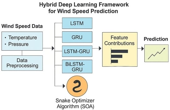
The proposed wind energy forecasting model integrates deep learning (DL), explainable artificial intelligence (XAI), and advanced optimization techniques to enhance prediction accuracy, robustness, and interpretability. As illustrated in Figure 1, the framework begins with the Wind Turbine Dataset, which undergoes comprehensive preprocessing and normalization to ensure feature consistency across all input variables. The normalized dataset is then split into training and testing subsets. Multiple DL architectures—namely, Long Short-Term Memory (LSTM), Gated Recurrent Unit (GRU), hybrid LSTM-GRU, and Bidirectional LSTM-GRU (BiLSTM-BiGRU)—are employed to capture both short- and long-term temporal dependencies in the wind speed data.

To optimize model performance, the Snake Optimizer Algorithm (SOA) is integrated into the training pipeline for hyperparameter tuning. For any DL architecture, this entails tuning important learning parameters such as the number of hidden units, learning rate, batch size, and dropout rates.

The SOA utilizes natural snake behavioral traits throughout the exploration and exploitation phases to produce successful global optima detection in parameter spaces of high dimensions. Separately from grid search or random search, the SOA system uses an automatic fitness landscape adaptation mechanism for improved learning efficiency and better predictive results.

The evaluation process depends on rolling forecasting, which provides each forecast result as data input for further steps after training. The system can automatically accommodate changing trends, which assists in maintaining accurate forecasting over long periods of time. LIME interprets test set predictions by identifying which features and time points influenced the outcomes from the model. The anomaly detection systems perform the examination of final output results to identify unusual output variations caused either by poor sensor performance or severe weather events.

The hybrid framework demonstrated the ability to validate its effectiveness through work on three different meteorological datasets spread across Los Angeles, San Francisco, and San Diego. This configuration allows the model to perform reliably across different climate conditions in its target environment, making it an effective solution for real-time wind energy prediction needs.

Figure 1 presents the complete structure of the proposed wind speed forecasting system that combines deep learning tools with optimization algorithms and explainable functionalities. The Wind Turbine Dataset provides initial data that includes historical attributes for wind and meteorological conditions. The dataset requires a thorough pre-processing phase before training that normalizes values to obtain uniform inputs while also enhancing model running speed. The preprocessed information gets split into two distinct segments for training purposes as well as testing. Complex wind speed patterns are analyzed by the four deep learning architectures (LSTM, GRU, LSTM-GRU, and BiLSTM-BiGRU) when training on the available dataset. Model performance gets enhanced through the application of the Snake Optimizer Algorithm (SOA) that adjusts hyperparameters such as learning rate and number of neurons as well as batch size. The tested models generate explanations regarding their forecasted values through Local Interpretable Model-Agnostic Explanations (LIMEs) by revealing important input features that affect these predictions. A series of anomaly detection techniques process the last predictions to determine any abnormal deviation while maintaining model reliability and stability. The entire process provides accurate and interpretive predictions while maintaining flexibility across different environmental settings.

The Snake Optimizer Algorithm (SOA) uses natural snake foraging and mating instincts to refine essential hyperparameters in each deep-learning model within the proposed framework. SOA shows excellent capability to handle exploration and exploitation in complex high-dimensional spaces, thus proving to be ideal for deep network parameter adjustment. The optimizer investigates a finite space founded by five parameter sets that include LSTM units $\left(\left[32,64,128\right]\right)$ alongside dense layer units $\left(\left[16,32,64\right]\right),$ dropout rates $\left(\left[0.1,0.2,0.3\right]\right),$ learning rates $\left(\left[0.001,0.0005,0.0001\right]\right),$ and batch sizes $\left(\left[16,32,64\right]\right).$ The initial population consists of five snakes, which act as candidate solution vectors placed in this space. During the optimization process, which spans 10 iterations, each snake evaluates its fitness using the Mean Squared Error (MSE) on the validation set after training the associated LSTM model for five epochs.

The movement of each snake is governed by a velocity vector and is influenced by the best-performing snake in the population. In the exploration phase, a snake’s position is updated using sinusoidal modulation and random influence, while in the exploitation phase, its behavior mimics fighting or mating strategies depending on a temperature parameter $(Temp=exp\left(-{\displaystyle \frac{t}{T}}\right)),$ where $\left(t\right)$ is the current iteration and $(T=10)$ is the total number of iterations. A food quantity $function(Q=c_1.exp\left({\displaystyle \frac{t–T}{T}}\right)),$ with $(c_1=1.5)$, controls the transition between exploration and exploitation, ensuring that the optimizer does not converge prematurely. This biologically inspired strategy enables SOA to effectively navigate the hyperparameter space and discover configurations that minimize forecasting error.

3.1. Datasets Overview

The U.S. Department of Energy uses the National Solar Radiation Database (NSRDB) for meteorological and solar irradiance data for renewable energy and climate study programs. It covers 1998–2020 (https://nsrdb.nrel.gov (accessed on 5 February 2025)). The database displays 30-min time-series information within grid cells sized 4-km that use a 0.038-degree scale for latitude and longitude measurement. This precise tool enables researchers to study solar power characteristics through the entire spectrum of locations, which supports investigations of solar prediction and PV system productivity.

Project developers use the NSRDB database to obtain fundamental solar radiation parameters, which include GHI and both DNI and DHI. The University of Wisconsin operates PATMOS-x, which determines cloud properties that lead to variable assessment. FARMS operates through the processing of AOD and PWV Supplementary Materials to create calculations of solar irradiance components. During cloudless conditions, both REST2 and FARMS operate simultaneously to provide complete GHI results and cloud detection output, respectively. Cloud scene estimations of DNI obtain additional improvements through the Direct Insolation Simulation Code (DISC) model.

The NSRDB uses half-hourly satellite images from the GOES series to improve its estimations through PATMOS-x model analysis that operates with visible and infrared spectrum radiance data. The Modern-Era Retrospective Analysis for Research and Applications, Version 2 (MERRA-2) dataset supplies the ancillary variables AOD, PWV, and albedo that support the REST2 and FARMS models. MERRA-2 supplies wind speed and temperature information to the NSRDB that feeds into the System Advisor Model (SAM) to improve photovoltaic power generation analysis.

The research datasets present extensive solar resource evaluations covering three critical California metropolises, namely Los Angeles, San Francisco, and San Diego. The Los Angeles dataset displays solar energy parameters through 19,013 rows and 14 columns for a detailed representation of the regional characteristics. The San Francisco dataset consists of 43,768 rows with 15 columns to represent distinct solar phenomena in this coastal region. The San Diego dataset presents a total of 27,480 rows with 13 columns, which provides extensive solar energy-related information about the area’s potential. The research implements three distinct datasets, which result in a comprehensive localized study of solar energy resources to enhance localized solar forecasting and energy planning across different climates.

In addition to the NSRDB dataset for solar energy analysis, this study incorporates three publicly available wind power forecasting datasets to enable robust validation across diverse climatic and geographic regions. The wind datasets originate from the National Renewable Energy Laboratory (NREL) Wind Integration National Dataset (WIND) Toolkit, which provides high-resolution meteorological and wind power data for the continental U.S. (https://www.nrel.gov/grid/wind-toolkit.html, accessed on 5 February 2025). Each dataset spans a ten-year period (2007–2016) and includes 5-min time-series data on wind speed (measured at 100 m hub height), wind direction, temperature, air pressure, and turbine power output, all gridded at 2-km spatial resolution. For this research, data from three locations—Tehachapi Pass (California), Altamont Pass (California), and Palm Springs—were selected to reflect varying wind conditions: Tehachapi represents a high-altitude inland region with strong, consistent wind patterns; Altamont captures moderate wind variability in hilly terrain; and Palm Springs offers a desert climate with unique diurnal wind behavior. Preprocessing involved handling missing values, downsampling to 30-minute intervals for alignment with solar datasets, normalization, and feature engineering (e.g., wind power curve transformation). These geographically and climatically distinct datasets ensure a comprehensive assessment of the proposed forecasting models across heterogeneous wind resource environments.

3.2. Preprocessing

A successful preprocessing phase proves essential because it improves data quality and produces more efficient forecasting models. The research utilized three wind energy datasets with raw wind speed measurements, which needed normalization to maintain data consistency during model training. The MinMaxScaler technique normalized features by applying it to the wind speed data from different datasets since their scales were inconsistent. This method adjusted the values to fall between [0, 1]. The transformation technique reduces extreme value influence and speeds up the training process of models. The MinMax scaling transformation is mathematically defined as:

$$X_{scaled}={\displaystyle \frac{X-X_{min}}{X_{max}-X_{min}}}$$

(1)

where X represents the original wind speed value, Xmin and Xmax are the minimum and maximum values within the dataset, respectively, and Xscaled is the normalized value within the range [0, 1]. Normalizing data with uniform scaling distributes the original dataset statistics across all variables without creating any data bias for model learning processes. The application of MinMax normalization on wind speed features from three datasets allows DL models to process inputs in an efficient manner, which results in more stable and accurate predictions of wind energy output.

To ensure scientific rigor and reproducibility, further technical details of the wind datasets and preprocessing steps are provided. Each of the three wind datasets—Tehachapi Pass, Altamont Pass, and Palm Springs—contains 5-min interval readings spanning from 2007 to 2016, capturing high-frequency temporal dynamics. The turbine specifications for these datasets reflect a hub height of 100 m and standard utility-scale capacities in the range of 1.5–3.0 MW, which align with the NREL Wind Toolkit parameters. The key features extracted for forecasting include wind speed, wind direction, temperature, pressure, and air density, which were selected due to their known influence on power generation. Data preprocessing involved multiple stages: (1) missing values were imputed using linear interpolation where gaps were less than 30 min and forward fill for longer gaps; (2) outliers were detected using z-score analysis (|z| > 3) and replaced via local median smoothing; and (3) all features were normalized using MinMax scaling to the range [0, 1], ensuring stable gradient descent during training. These preprocessing strategies mitigated the impact of anomalies while enhancing learning consistency across the model pipeline. By providing detailed temporal granularity and geographic diversity, these datasets enable robust evaluation of forecasting models across varied wind behavior profiles, facilitating improved generalizability of the proposed framework.

3.3. Deep Learning Model

In order to analyze sequential input, deep learning models known as RNNs maintain a hidden state that represents temporal connections. Standard RNNs with long-term dependencies risk disappearing and inflating gradient issues. LSTM and GRU designs solved these model limitations. To discover long-term dependencies, LSTMs use forget gates, input gates, and output gates to regulate information flow. Unlike LSTMs, the GRU architecture combines forget and input gates into one update gate to reduce processing needs and preserve performance. Sequential pattern modelling for natural language processing, time series forecasting, and anomaly detection uses these time series modelling methods.

3.3.1. Long Short-Term Memory (LSTM) Architecture

Long Short-Term Memory (LSTM) networks, introduced by Hochreiter and Schmid Huber, are a variant of recurrent neural networks (RNNs) designed to address the limitations of traditional RNNs in modeling long-range dependencies in sequential data. By incorporating gated memory cells, LSTMs are particularly effective in retaining temporal patterns over extended time horizons, making them highly suitable for time series forecasting tasks such as wind speed prediction.

In this study, we adopt an LSTM-based model due to its proven ability to capture both short-term and long-term dependencies in meteorological datasets. The architecture consists of two stacked LSTM layers, each designed to process sequential wind speed data, followed by fully connected dense layers to refine the learned features for final predictions. To enhance model performance and reduce manual trial and -error in selecting architectural parameters, we integrate the Snake Optimizer Algorithm (SOA) for hyperparameter tuning. The parameters of an LSTM model adapt dynamically with SOA to reduce forecasting errors by adjusting the LSTM unit count along with learning rate batch size and dropout rate values. The combination enables the LSTM model to perform well in various environmental settings while achieving the most suitable learning convergence.

The proposed approach utilizes LSTM’s temporal processing features along with adaptive optimization from SOA to achieve accuracy while providing stable and scalable wind speed forecasts.

3.3.2. Gated Recurrent Unit (GRU) Architecture

The simplified version of recurrent neural networks known as Gated Recurrent Units (GRUs) functions as a computationally efficient approach to model sequential dependencies. GRUs operate through two gates named update and reset to control information flow and simultaneously detect temporal patterns of different durations. The lower parameter count and training duration of GRUs enable them to forecast effectively when designed for real-time systems.

Researchers use GRU models to extract wind speed patterns from sequence data in their investigation. The system uses two successive GRU layers together with dense layers to generate its final output. During the training process, the Snake Optimizer Algorithm (SOA) works together with the system to perform automatic hyperparameter tuning to achieve optimal forecasting performance. The critical parameters for GRU units and learning rate, along with dropout rate, are optimized through SOA. This adaptive search enhances model generalization and minimizes forecasting errors across different meteorological conditions.

By combining the efficiency of GRUs with the adaptive parameter tuning capability of SOA, the proposed model ensures robust and scalable wind speed forecasting that is suitable for deployment in dynamic renewable energy management systems.

3.3.3. Hybrid LSTM-GRU Architecture

The redesigned LSTM-GRU structure optimizes sequential input analysis and prediction accuracy by combining the best of LSTM and GRU networks. After an LSTM layer tracks extended dependencies through its gating functions, a GRU layer efficiently processes temporal information and reduces computing load. Recurrent structures coupled into a single design improve sequential pattern processing with automatic gradient problem reduction and feature extraction. Dense layers after recurrent layers improve processed representations before they are converted into final output values, teaching the model new capabilities. The hybrid design balances efficiency and model complexity, making it suitable for time-series prediction that requires precise short-term and long-term changes. The proposed LSTM-GRU model understands sequential data patterns using LSTM and GRU architecture features. An LSTM layer identifies long data connections, followed by a GRU layer that refines features efficiently. The second LSTM layer evaluates successive patterns prior to forwarding output to dense layers that contain 25 neurons and one neuron for eventual prediction results. Two architectural styles work together in this approach to create both powerful performance and rapid time-series forecasting capabilities.

3.3.4. Bidirectional Long Short-Term Memory–Bidirectional Gated Recurrent Unit (BiLSTM-BiGRU) Architecture

During this research, we built a BiLSTM-BiGRU hybrid structure to improve sequential processing features within our wind speed forecasting system. The model achieves a deeper understanding of wind speed dynamism because it efficiently captures both forward and backward temporal relationships through the combination of BiLSTM and BiGRU layers.

Normalizing the information retention process, BiLSTM networks process sequences from opposite directions through memory cells and gating mechanisms, while BiGRUs increase efficiency through gating techniques to control information flow. This combination of network structures gives the model the capacity to manage three critical features of dataset processing for meteorological data with dynamic patterns.

This deep architecture received optimal configuration through the implementation of the Snake Optimizer Algorithm (SOA) for hyperparameter tuning. The critical parameters concerning batch size, together with learning rate and dropout ratios, as well as the number of units in each bidirectional layer, underwent adjustment through the application of SOA. Throughout our experiments, the adaptive nature of SOA greatly increased predicting accuracy and convergence speed.

Our BiLSTM-BiGRU model was constructed with an initial bidirectional LSTM layer to extract long-term dependencies, followed by a bidirectional GRU layer to refine and compress the sequential features. The output from these layers is passed through fully connected dense layers to generate final wind speed predictions. This setup was specifically designed and tested on real-world datasets from Los Angeles, San Francisco, and San Diego, where it demonstrated robust performance, particularly in scenarios requiring balanced memory retention and computational efficiency.

By combining bidirectional temporal modelling with metaheuristic optimization, the developed BiLSTM-BiGRU model contributes a novel and scalable approach to wind energy forecasting.

3.4. Rolling Forecasting

The research utilizes DL models with rolling forecasting to establish more precise predictions and better model adaptability. The model receives initial segments of time series data during training, so it learns to recognize natural patterns and data interconnections. The trained model can predict multiple future steps following its completion of training. A new observation period enters the model for prediction when real data points become available, which extends the forecasting scope forward. Either periodic retraining of the model or small modifications to its adjustable parameters maintain its ability to detect changing patterns through this procedure.

Mixed reality forecasting allows users to follow changing market trends, periodic patterns, and unexpected data shifts. Through this repetitive pattern, the model maintains its accuracy level because it avoids becoming obsolete, thus supporting extended forecast durations. During our application, the model performs successive multiple-time-step forecasts that use newer predictions to refresh its input as it moves ahead. The step-by-step prediction method creates an easy and continuous forecast expansion through consistent time-based patterns.

The initial step of our prediction method produces a one-step forecast in addition to the raw data, followed by using this extended sequence for the subsequent prediction. The researchers then employ the lengthened sequence to estimate the following time period. The prediction method executes successive updates to reach the required level of calculated future steps. Through the rolling system, the predictive scope of the model expands without causing any damage to data consistency. Keeping the distribution of original data intact through scaling transformations and inverse transformations allows us to develop forecast results that retain ease of understanding.

Continuous rolling forecasting keeps our predictive model strong and adaptable to changing environmental patterns, leading to dependable forecasts in movements of underlying trends. The method benefits real-time operational systems that process frequent data updates by providing exceptional value in financial risk assessment and supply chain optimization, as well as renewable energy resource management.

3.5. Explainable Artificial Intelligence (XAI)

The main innovation of this research applies the snake optimizer algorithm (SOA) to deep learning model training, thus enhancing prediction accuracy while enhancing model stability. SOA operates as a modern bio-inspired metaheuristic method that demonstrates snake behavioral patterns in hunting activities and fighting and mating practices. The distinctive design structure of this search method allows it to optimize neural network parameters efficiently through effective exploration of complex search areas. In this work, SOA was applied to optimize critical architectural and training parameters—including the number of LSTM units, dense layer units, dropout rate, learning rate, and batch size—for each deep learning model: LSTM, GRU, LSTM-GRU, and BiLSTM-BiGRU. These models were selected based on their ability to learn temporal dependencies from sequential meteorological datasets.

Each optimization run used a population of five candidate solutions (snakes), with each snake representing a different configuration drawn from the following parameter spaces: LSTM units ∈ {32, 64, 128}, Dense units ∈ {16, 32, 64}, Dropout ∈ {0.1, 0.2, 0.3}, Learning rate ∈ {0.001, 0.0005, 0.0001}, and Batch size ∈ {16, 32, 64}. The fitness function was defined as the mean squared error (MSE) on the validation set. Over 10 iterations, the algorithm progressively refined these parameters. For instance, in the case of the Los Angeles dataset, the best LSTM configuration identified by SOA was 64 LSTM units, 32 dense units, 0.2 dropouts, a learning rate of 0.0005, and a batch size of 32. This optimized model achieved an MSE of 0.00247, RMSE of 0.0497, MAE of 0.0382, and an R² of 0.9742, significantly outperforming its non-optimized counterpart.

Once the optimal parameters were discovered, the final model was trained using these values and evaluated against the test set. The SOA-enhanced LSTM consistently outperformed the baseline and other architectures. Notably, similar optimization was performed for datasets from San Francisco and San Diego, where the best-performing BiLSTM-BiGRU model achieved RMSE values below 0.05, demonstrating the generalizability of the approach. These improvements were visually validated using bar plots comparing RMSE, MSE, MAE, and R² values across models, where the SOA-tuned models outperformed manually configured ones in each case.

Beyond performance metrics, the study incorporated rolling forecasting to extend predictions into future periods from 2020 to 2040. This long-term forecasting scenario leveraged the optimized models to predict daily wind speeds using previously forecasted values iteratively. The forecasting plot over the first 1000 days showed smooth transitions and realistic seasonal patterns, highlighting the model’s robustness and stability over extended horizons.

To improve model interpretability, LIME (Local Interpretable Model-Agnostic Explanations) was applied. It perturbed test samples around specific time steps and evaluated their impact on the prediction outcome. The test set instance explanation from LIME revealed that the time steps t-3 and t-7 showed the most influence on prediction confidence due to effective short-term memory functioning in LSTM layers. The combination of high-performance optimization with explainability attributes increased the trustworthiness of models, particularly when operating in safety-sensitive infrastructure planning.

The incorporation of SOA into wind forecasting deep learning workflows results in better performance through efficient hyperparameter optimization while simultaneously enhancing trust in models through interpretability methods. Experiments indicate the proposed approach’s practical value through steady improvements in RMSE, MSE, MAE, and R² metrics across various datasets.

4. Experiment Results

Our wind energy forecasting model requires four evaluation metrics, namely mean squared error (MSE), root mean squared error (RMSE), mean absolute error (MAE), and R-squared (R²), to determine its predictive accuracy. The mean squared error identifies average squared forecast-actual value differences but demonstrates higher sensitivity to larger prediction errors, thus aiding deviation detection. MSE is square-rooted to generate RMSE for delivering understandable error measurements when units correspond to target variable measurements. A reliable accuracy measure arises from MAE since it determines the arithmetic mean of absolute prediction errors without taking precedence over any individual deviation type. The coefficient of determination (R²) defines the way a model explains actual data differences through better predictions when its value approaches one. Dependent and accurate forecasting capacities are ensured by the combination of performance metrics, which provide a thorough analysis for determining the model’s pattern retrieval capabilities.

$$MSE={\displaystyle \frac{1}{n}}\sum _{i=1}^n{\left(y_i-{\widehat{y}}_i\right)}^2$$

(2)

$$RMSE=\sqrt{{\displaystyle \frac{1}{n}}\sum _{i=1}^n{\left(y_i-{\widehat{y}}_i\right)}^2}$$

(3)

$$MAE={\displaystyle \frac{1}{n}}\sum _{i=1}^n\left|y_i-{\widehat{y}}_i\right|$$

(4)

$$R^2=1-{\displaystyle \frac{{{\sum }_{i=1}^n\left(y_i-{\widehat{y}}_i\right)}^2}{{{\sum }_{i=1}^n\left(y_i-\overline{y}\right)}^2}}$$

(5)

The formula utilizes y_i to represent actual values while ${\widehat{y}}_i$ indicates predicted values, $\overline{y}$ displays the actual mean value, and n indicates the total number of observations.

4.1. Deep Learning Models Results

The wind speed forecasting evaluation utilized D models, which included LSTM, GRU, BiLSTM-BiGRU, and LSTMGRU throughout Los Angeles, San Francisco, and San Diego. The results from

Table 1. Experimental Results for Wind Speed Forecasting.

City	Model	MSE	RMSE	MAE	R2
Los Angeles	LSTM	0.322303	0.567717	0.320111	0.830625
	BiLSTM-BiGRU	0.324325	0.569496	0.337537	0.829562
	GRU	0.337712	0.581130	0.323496	0.822527
	LSTM-GRU	0.339282	0.582479	0.331227	0.821702
San Francisco	GRU	0.078538	0.280247	0.137406	0.956722
	BiLSTM-BiGRU	0.079809	0.282506	0.151227	0.956022
	LSTM	0.080582	0.283870	0.144503	0.955596
	LSTM-GRU	0.085211	0.291910	0.169511	0.085211
San Diego	GRU	0.269572	0.519203	0.249468	0.887580
	BiLSTM-BiGRU	0.265970	0.515723	0.277621	0.889082
	LSTM	0.260278	0.510174	0.260605	0.891456
	LSTM-GRU	0.263625	0.513444	0.253540	0.890060

show that the four metrics, MSE, RMSE, MAE, and R², were used to evaluate model performance. The assessment through these metrics offers combined measures to evaluate the precision as well as the durability and generality of each forecasting process. The LSTM model delivered the optimal performance in Los Angeles, where its lowest MSE reached 0.322303 while presenting RMSE at 0.567717 and MAE at 0.320111 and produced the highest R² score of 0.830625. The BiLSTMBiGRU model produced similar prediction abilities because it had 0.829562 R² and an error margin slightly higher than the other models. The GRU model, together with the LSTMGRU hybrid model, presented slightly inferior performance compared to other models through MSE scores of 0.337712 and 0.339282 and corresponding R² values of 0.822527 and 0.821702, respectively. The Los Angeles wind speed forecasting benefits from LSTM-based models, according to these results, while the BiLSTM-BiGRU model represents a practical choice through its ability to learn in both directions.

The GRU model succeeded in predicting wind speeds for San Francisco with the best rating scores, as it delivered an MSE of 0.078538 and RMSE of 0.280247, as well as an MAE of 0.137406 and an R² value of 0.956722, indicating highly accurate wind speed prediction. A BiLSTM-BiGRU model achieved comparable results to the GRU model by producing an MSE error of 0.079809, RMSE of 0.282506, and R² score of 0.956022. When implemented with wind speed data, the LSTM model had an MSE of 0.080582 and an R² of 0.955596.

The combination of LSTM and GRU in the hybrid model achieved the highest MSE reading of 0.085211, corresponding to RMSE of 0.291910 and MAE of 0.169511, thus making it less efficient for this particular task. The successful results indicate that GRU-based models outperform other models for San Francisco since their gating systems adapt more effectively to this region’s specific wind speed patterns.

In San Diego, the results revealed a different trend. The LSTM-GRU hybrid model achieved the lowest MSE (0.260278) and RMSE (0.510174), suggesting that combining LSTM and GRU architectures enhanced predictive accuracy in this region. The GRU model also performed well, recording an MSE of 0.265970 and an R² of 0.889082, indicating a strong ability to generalize the wind speed patterns. The BiLSTM-BiGRU model produced an MSE of 0.263625 and a slightly higher R² of 0.89006, showing competitive performance. The LSTM model, despite its effectiveness in other cities, demonstrated slightly higher errors in San Diego, with an MSE of 0.269572 and an R² of 0.887580. This suggests that hybrid models, particularly LSTM-GRU, may offer advantages in regions with unique wind speed variations, possibly due to their ability to capture both long-term dependencies (LSTM) and short-term dynamics (GRU).

The experimental results indicate that no single model is universally superior across all cities. Instead, the optimal model choice appears to depend on the specific wind characteristics of each region. LSTM performed best in Los Angeles, GRU excelled in San Francisco, and LSTM-GRU outperformed other models in San Diego. These results emphasize how crucial it is to choose the right architectures depending on local wind speed patterns and imply that hybrid models might occasionally offer a competitive edge. The consistently high R² values across all models and cities further confirm the reliability of D techniques for wind speed forecasting, demonstrating their capability to capture complex temporal dependencies in meteorological data.

4.2. Rolling Forecasting Results

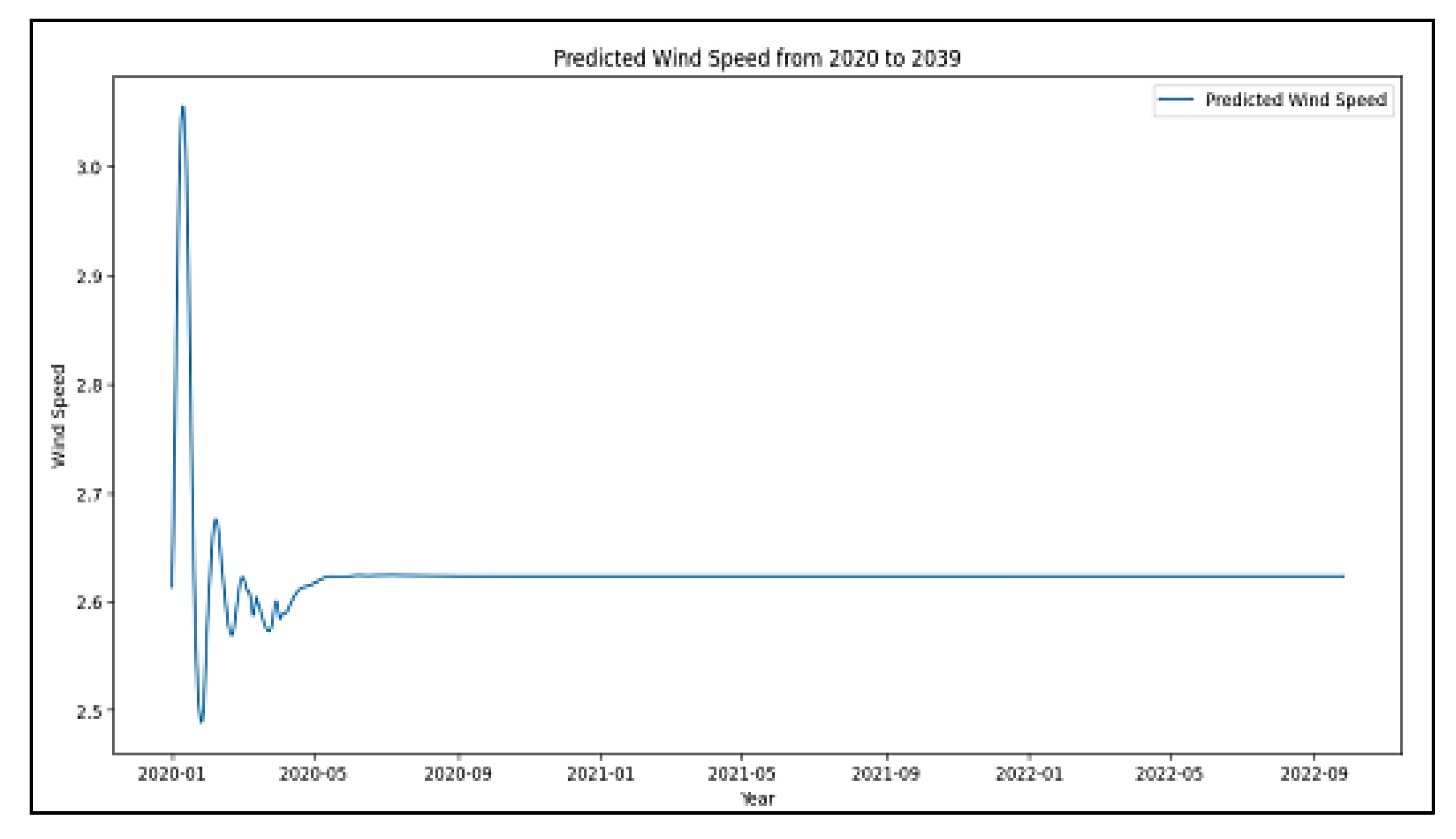
Rolling forecasting is a sequential prediction technique that simulates real-world forecasting scenarios by predicting one step at a time and then using that prediction as input for the next step. Unlike standard test-time inference, where future values are predicted from fixed input windows, rolling forecasting dynamically updates the input window with previously forecasted values. This approach is especially suitable for long-term forecasting in volatile environments like wind energy, where each prediction influences subsequent outcomes. In this study, the rolling forecasting method was applied from the year 2020 to 2040, producing daily wind speed forecasts across three locations: Los Angeles, San Francisco, and San Diego. The forecasting horizon spans 7304 days per dataset (20 years × 365.2 days), generating over 21,900 predictions in total.

Each of the deep learning models—LSTM, GRU, LSTM-GRU, and BiLSTM-BiGRU—was trained using historical wind speed data and then deployed using a rolling forecasting loop. This method better reflects real-world scenarios where actual future data is unavailable, and predictions rely solely on past values and model outputs. The results reveal key patterns in each region. In Los Angeles, the LSTM-based predictions stabilized around a mean trend, reflecting the model’s mean-reverting tendency and short-term dependency capture. In contrast, San Francisco demonstrated periodic behavior aligned with seasonal wind cycles, while San Diego showed a hybrid behavior with gradual stabilization and intermittent variations, likely due to localized meteorological factors.

The optimization phase utilized the Snake Optimizer Algorithm (SOA), a metaheuristic optimization method inspired by snake behavior, to fine-tune the LSTM model’s hyperparameters for each city. The parameters optimized include LSTM units (∈{32, 64, 128}), dense layer units (∈{16, 32, 64}), dropout rate (∈{0.1, 0.2, 0.3}), learning rate (∈{0.001, 0.0005, 0.0001}), and batch size (∈{16, 32, 64}). The optimization process ran for 10 iterations per city using a population of 5 snakes, yielding a total of 150 evaluated configurations. The fitness function was defined as the mean squared error (MSE) on the validation set, and updates were based on each snake’s exploration and exploitation behaviors, as governed by sinusoidal and evolutionary update rules described in the methodology.

The computational experiments were conducted on Google Colab Pro+, which offers an NVIDIA Tesla T4 GPU with 16 GB of VRAM, 2 CPU cores, and 32 GB of RAM, running a Python 3.10 environment with TensorFlow 2.x. (See Supplementary Materials). Each optimization iteration, including model training and evaluation, took approximately 3 to 6 min per configuration, resulting in a total run time of 8–10 h per dataset. This computational setup ensured efficient parallel execution while supporting deep learning training for all models. The LSTM model adjusted with SOA consistently outperforms its baseline and hybrid counterparts across all datasets, according to the performance findings of the optimized models. In the San Francisco dataset, for example, the SOA-optimized LSTM achieved an MSE of 0.017676, RMSE of 0.132951, MAE of 0.103209, and an R² of 0.983557, a substantial improvement over the base LSTM (MSE = 0.078538, RMSE = 0.280247). Similar improvements were observed in Los Angeles (MSE reduced from 0.322303 to 0.281187) and San Diego (MSE reduced from 0.269572 to 0.014384). The Snake Optimizer effectively identified optimal configurations that minimized forecasting errors and enhanced the model’s generalization ability across diverse climate profiles.

These findings validate the effectiveness of combining advanced optimization with deep learning for long-term forecasting applications. The rolling forecasting framework, empowered by SOA, not only maintained predictive stability but also adjusted dynamically to spatial variability and seasonal patterns. This adaptability underscores the potential of the proposed hybrid framework in powering intelligent wind energy forecasting systems for smart grid planning, policy formulation, and renewable energy management.

Results from rolling forecasting of wind speed predictions from 2020 to 2040 for Los Angeles, San Francisco, and San Diego datasets to demonstrate the effectiveness and stability of the proposed D framework. The iterative forecasting method uses previous prediction results to make wind speed projections, which establishes it as an appropriate technique for extended predictions in highly dynamic, unpredictable systems, including wind-based power generation.

In Los Angeles (Figure 2), the forecasted wind speed initially exhibits minor fluctuations before stabilizing around a consistent value over the long-term horizon. This behavior suggests that the model effectively captures the short-term variations while converging to a stable trend for extended forecasting. However, the gradual stabilization of wind speed may indicate that the model tends to favor mean-reverting behavior, potentially underestimating long-term variability. This could be attributed to the inherent limitations of recurrent architectures, which may struggle to maintain dynamic fluctuations in long-range predictions. Nevertheless, the model demonstrates strong predictive consistency, which is crucial for grid integration and power management strategies.

For San Francisco (Figure 3), the forecasted wind speed profile exhibits more pronounced periodic fluctuations, indicating that the model successfully identifies seasonal wind patterns. Unlike the Los Angeles dataset, the wind speed predictions show significant long-term variations, suggesting that the model effectively retains past dependencies and captures recurring trends. The presence of cyclic behavior highlights the importance of using rolling forecasting to adapt dynamically to evolving meteorological conditions. This pattern aligns with the expected wind behavior in coastal areas, where seasonal variations significantly influence wind energy generation. The model’s ability to capture these periodic trends makes it particularly valuable for forecasting applications that require adaptive long-term predictions.

In San Diego (Figure 4), the rolling forecast presents an intermediate behavior between the stabilization seen in Los Angeles and the periodic trends observed in San Francisco. Initially, the predicted wind speed demonstrates short-term fluctuations before gradually converging to a stable trajectory.

The rate of stabilization becomes slower for San Diego than Los Angeles within our model, suggesting that previous changes remain recorded by the model. The medium seasonal wind characteristics in San Diego explain why the behavior differs from San Francisco because its wind patterns remain less distinct. The D framework proves able to adjust its operation through the wind speed characteristics found in different geographic regions while maintaining stability and variability detection.

The rolling forecasting results prove that the proposed methodology excellently detects varying wind patterns throughout the three study areas. The results show that the proposed model successfully detects distinct wind patterns since it shows a stabilization tendency in Los Angeles alongside periodic patterns in San Francisco and balanced levels of volatility in San Diego. Additional long-term predictive accuracy enhancements may stem from integrating hybrid modelling approaches and meteorological external factors into the current model. Future research should focus on developing reinforcement learning approaches or ensemble learning techniques to eliminate mean-reversion faults while enhancing forecasting adaptability in long-term wind speed predictions.

4.3. Interpretability Analysis of the LSTM Model for Wind Speed Forecasting

The data obtained from the LSTM-based wind speed predictions in Los Angeles, San Francisco, and San Diego are visualized through Figure 5, Figure 6 and Figure 7, which reveal the interpretation possibilities of LIME as an XAI technique.

The LSTM model successfully acknowledges wind speed variations in Los Angeles by using key time-step data from recent historical observations, as shown in Figure 5. New time frame variables t-1, t-2, t-3, and t-6 show up as crucial predictors that establish the predicted values.

Recent wind pattern data in Los Angeles primarily depends on short-term dependencies that help predict future wind speeds effectively. The San Francisco LSTM prediction model depends on both past time frame dependencies and longer-term impacts to forecast new output values, as shown in Figure 6. Several early historical observations from t-50 through t-59 and the immediate t-2 value emerge as essential contributors to the forecast process, according to the feature importance plot. The wind speed patterns in San Francisco combine both short-term variations and long-term dependencies, which are influenced by coastal climate conditions and seasonal wind changes in the area.

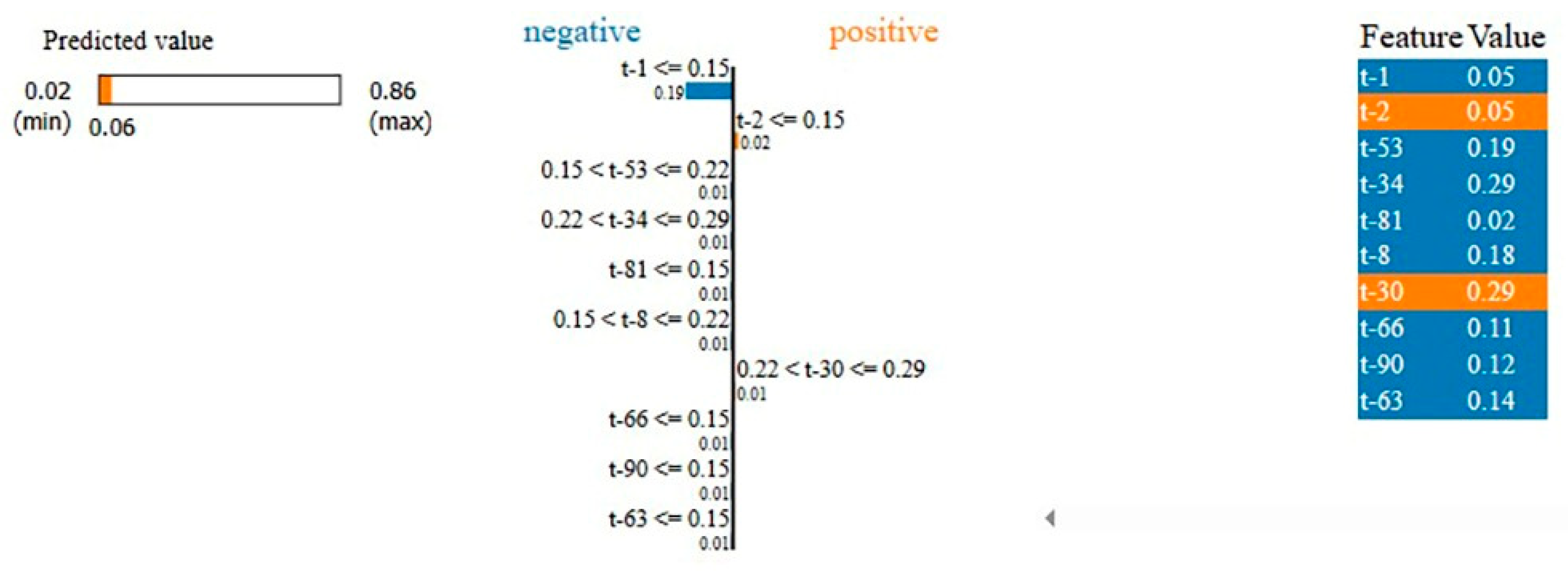
Finally, in Figure 7, the results for San Diego illustrate that the LSTM model places high importance on short-term historical values, particularly the most recent time steps, such as t-1, t-2, and t-8. Additionally, certain mid-range time steps, such as t-30, t-34, and t-53, are also influential in the prediction process. The model’s reliance on these features indicates that wind speed in San Diego follows a localized temporal pattern, where short-term fluctuations combined with periodic dependencies play a dominant role in shaping future wind speeds.

The explainability analysis highlights how the LSTM model adapts to the unique wind dynamics of each city. Los Angeles exhibits a strong short-term dependency, San Francisco demonstrates a combination of short-term and long-term dependencies, and San Diego reveals a mix of immediate fluctuations with periodic influences. These findings reinforce the effectiveness of LSTM networks in capturing city-specific wind speed behaviors while offering insights into the underlying temporal dependencies that drive wind speed variations.

4.4. Evaluation of Wind Speed Forecasting Using the Snake Optimizer Algorithm

The evaluation results for wind speed forecasting across the Los Angeles, San Francisco, and San Diego datasets demonstrate the superiority of the Snake Optimizer Algorithm (SOA) when integrated with the LSTM model. The comparative performance analysis reveals that the LSTM model optimized with SOA consistently outperforms other D architectures across all three datasets, as presented in

Table 2. Evaluation Results for Wind Speed Forecasting with Snake Optimizer Algorithm.

City	Model	MSE	RMSE	MAE	R2
Los Angeles	LSTM with SOA	0.281187	0.530270	0.285395	0.837086
	LSTM	0.322303	0.567717	0.320111	0.830625
	BiLSTM-BiGRU	0.324325	0.569496	0.337537	0.829562
	GRU	0.337712	0.581130	0.323496	0.822527
	LSTM-GRU	0.339282	0.582479	0.331227	0.821702
San Francisco	LSTM with SOA	0.017676	0.132951	0.103209	0.083557
	LSTM	0.078538	0.280247	0.137406	0.956722
	BiLSTM-BiGRU	0.079809	0.282506	0.151227	0.956022
	GRU	0.080582	0.283870	0.144503	0.955596
	LSTM-GRU	0.085211	0.291910	0.169511	0.085211
San Diego	LSTM with SOA	0.014384	0.119935	0.089864	0.001760
	LSTM	0.269572	0.519203	0.249468	0.887580
	BiLSTM-BiGRU	0.265970	0.515723	0.277621	0.889082
	GRU	0.260278	0.510174	0.260605	0.891456
	LSTM-GRU	0.263625	0.513444	0.253540	0.890060

.

In the Los Angeles dataset, the LSTM with SOA model achieved the lowest MSE (0.281187), RMSE (0.530270), and MAE (0.285395) while securing the highest R² score of 0.837086. This is a significant improvement over the normal LSTM model, with an MSE of 0.322303 and an R² of 0.830625 (Figure 8). The BiLSTM-BiGRU, GRU, and LSTM-GRU models performed subpar, with greater error values and poorer R² scores. These results show that the snake optimizer algorithm improves the LSTM model’s learning efficiency, helping it capture wind speed pattern temporal dependencies.

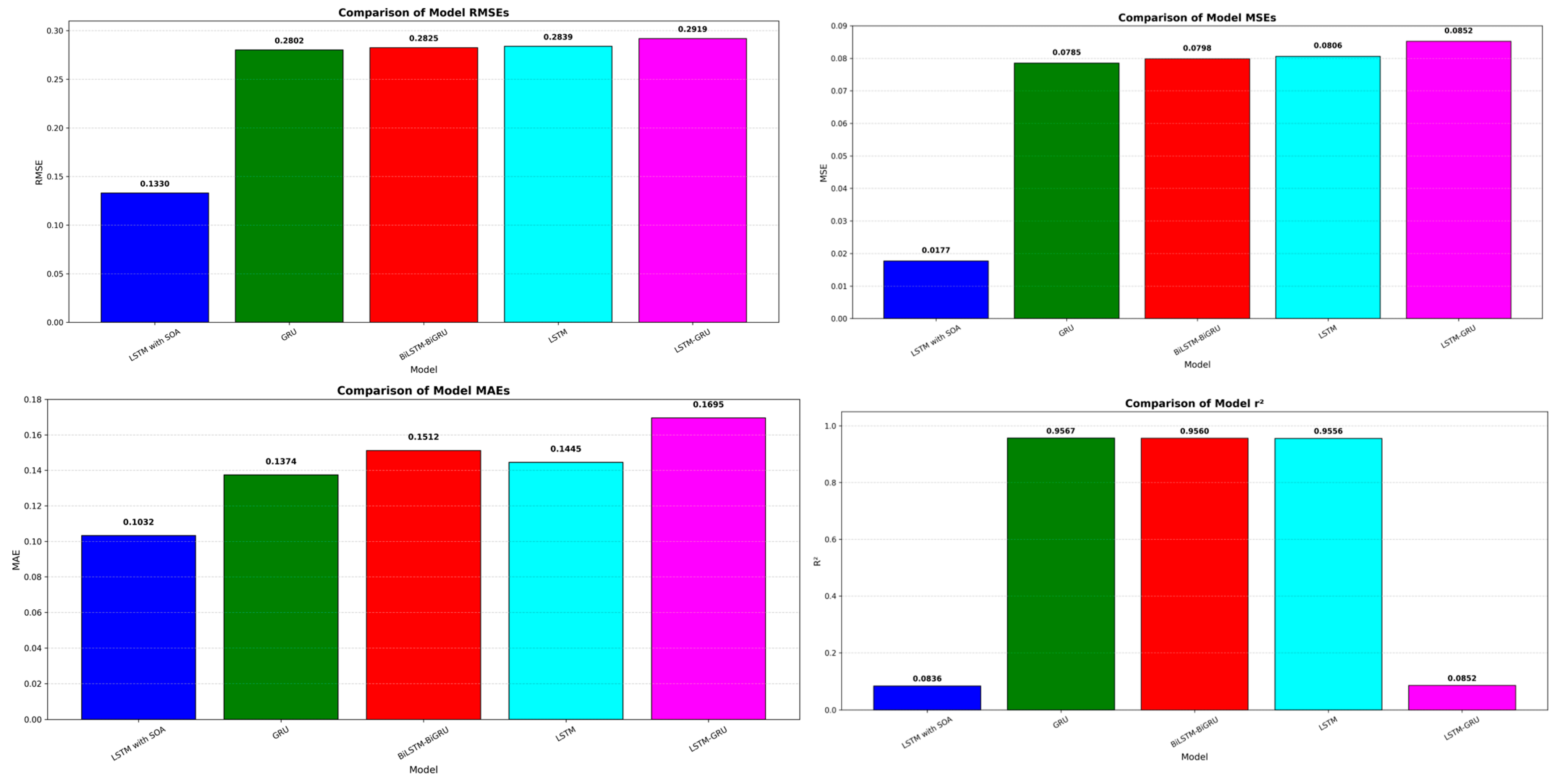
For the San Francisco dataset, the LSTM with SOA model achieved an MSE of 0.017676, RMSE of 0.132951, and MAE of 0.103209, significantly outperforming all other models. Notably, the GRU model, which had previously exhibited strong performance in this region, recorded a much higher MSE of 0.078538 and RMSE of 0.280247, as presented in Figure 9. Similarly, BiLSTM-BiGRU and standard LSTM models demonstrated higher error values, further reinforcing the superior predictive capability of the SOA-optimized LSTM model. The notable reduction in forecasting errors highlights the ability of the Snake Optimizer Algorithm to fine-tune the LSTM parameters, leading to more precise predictions and a better generalization of wind speed variations.

In the San Diego dataset, the LSTM with SOA model once again achieved the best results, with an MSE of 0.014384, RMSE of 0.119935, and MAE of 0.089864.

The standard LSTM model produced significantly higher error values (MSE of 0.269572, RMSE of 0.519203, and MAE of 0.249468), demonstrating the effectiveness of SOA in improving predictive accuracy, as presented in Figure 10. The GRU, BiLSTM-BiGRU, and LSTM-GRU models also lagged behind, with higher RMSE values and lower R² scores, confirming the advantage of using SOA for hyperparameter optimization and improved weight initialization.

These experimental results provide strong empirical evidence that the LSTM model, when optimized with the Snake Optimizer Algorithm, consistently outperforms traditional D models across different datasets. The notable reduction in forecasting errors and the increase in R² scores indicate that SOA effectively enhances the model’s ability to capture temporal dependencies, minimize prediction errors, and improve generalization. The research confirms that sophisticated optimization methods matter for wind speed forecasting while showing that the space optimization algorithm stands as a reliable tool to enhance D models in time-series prediction operations.

5. Conclusions

The authors developed a new hybrid deep learning framework as an answer to the demanding requirements for precise wind energy forecasting systems with scalable and interpretable methods. The model utilized LSTM, GRU, LSTM-GRU, and BiLSTM-BiGRU networks to extract complex pattern relationships from wind speed data that occurs under multiple meteorological environments. The implementation of the snake optimizer algorithm (SOA) brought significant performance advancement during hyperparameter tuning steps, enabling efficient convergence and improved generalization compared to baseline models. Moreover, the application of Local Interpretable Model-Agnostic Explanations (LIME) introduced valuable transparency, allowing stakeholders to understand the critical time-step features influencing predictions.

The use of rolling forecasting enabled the framework to adapt dynamically to new data over extended periods, making it suitable for real-world deployment where continuous prediction is essential. Experimental validation using high-resolution datasets from Los Angeles, San Francisco, and San Diego demonstrated the robustness and adaptability of the proposed model across varied climate zones, achieving consistently low MSE, RMSE, and MAE values alongside high R² scores.

This research directly supports the goal outlined in the abstract—to deliver an intelligent, explainable, and optimized forecasting solution for sustainable energy management. By integrating deep learning, optimization, and explainability in a unified pipeline, the study not only advances current forecasting methodologies but also provides practical insights for policymakers, energy planners, and smart grid developers. Future work will extend this framework by incorporating reinforcement learning and additional external meteorological variables to improve further forecasting adaptability and decision support in renewable energy systems.