1. Introduction
Solar energy, as a clean and renewable resource, is playing an increasingly vital role in the global energy structure. Due to the serious challenges of climate change and environmental degradation, taking full advantage of sustainable energy resources and achieving green, low-carbon development has become a global consensus [
1]. The proposal of the Paris Agreement [
2] and “dual carbon” targets [
3] push forward the reduction in greenhouse gas emissions and accelerate the integration of renewable energy. Under these circumstances, photovoltaic (PV) power generation has emerged as a key driver of the global energy transition, owing to its advantages of low carbon emissions, pollution-free operation, and abundant resource availability. Thus, the installation and integration of PV systems is growing rapidly [
4,
5,
6]. However, the output of PV power generation is fluctuating and intermittent, which is largely influenced by factors such as solar radiation, temperature, and humidity. The uncertainty of PV power generation poses significant challenges to grid stability and energy management. Therefore, the accurate prediction of PV power generation is crucial for maximizing integration capacity, ensuring efficient power dispatch, and optimizing energy utilization [
7,
8,
9].
Generally, photovoltaic power generation forecasting methods are classified into indirect methods [
10] and direct methods [
11,
12]. The indirect forecasting method, also known as the physical forecasting method, is based on weather forecast information provided by meteorological stations. It requires the data of solar irradiance, wind speed, humidity, and temperature. The installation angle and location of photovoltaic panels, as well as the conversion efficiency of solar cells, are also needed. A physical model is constructed with the above parameters. Photovoltaic power generation for a specific time period can be calculated using the physical model and relevant formulas [
13,
14]. AlamS et al. [
15] employed three broadband irradiance models to predict solar irradiance at four sites in India. The accuracy of each model was evaluated by comparing the calculated direct normal irradiance and global irradiance with reference and measured values. TaoK et al. [
16] combined transformer-based physical modeling with data-driven forecasting methods by introducing PV-related transformer variables (such as current, voltage, etc.) as key features and using physical parameters to model the relationship between environmental conditions and PV module output. Finally, historically observed data and weather forecasting data are used in conjunction with a data-driven temporal feature extraction network to achieve multi-step forecasting. In another study, a dynamic physical modeling method called PVPro to achieve high-accuracy short-term power forecasting is introduced [
17]. It adjusts the model parameters based on recent production data to convert environmental data into PV system output power. SinglaP et al. [
18] and ArimatsuK et al. [
19] constructed approximate physical models of photovoltaic power generation and established equivalent circuit models of photovoltaic arrays. These models calculate the output power of photovoltaic systems based on the electrical characteristics of solar cells and environmental factors, which are also combined with variables such as solar irradiance and temperature. However, although the indirect forecasting method does not require detailed historical data to train the forecasting model, it relies heavily on the detailed geographic information of power stations and accurate meteorological data. Moreover, physical formulas have certain errors. These errors lead to poor resistance to interference and weak robustness [
10].
Direct forecasting methods include statistical forecasting methods and artificial intelligence forecasting methods. Statistical forecasting methods use historical data on weather, solar radiation, etc., to perform curve-fitting and establish an input–output mapping model for photovoltaic power generation forecasting [
20]. In an experimental study, a method based on the Markov chain model to predict the short-term output power of photovoltaic systems is presented [
21]. By analyzing historical data from photovoltaic power stations, a mathematical statistical model was constructed, which effectively improved the accuracy of output power prediction under dynamic changes in the solar environment. LiY et al. [
22] propose an ARMAX model, which combines historical power output data from photovoltaic systems with external meteorological factors to predict the short-term output power of grid-connected photovoltaic systems. YooE et al. [
23] introduced a federated learning algorithm based on fuzzy clustering, which improves the accuracy and flexibility of solar power forecasting by clustering data between distributed generators. Since statistical forecasting methods do not need to consider the installation conditions of photovoltaic panels and the conversion efficiency of photovoltaic arrays, they are simpler to implement compared with physical methods. However, most statistical forecasting methods are linear, which is unfavorable for long-term or large-scale photovoltaic power generation prediction. The models rely on large amounts of effective historical data, which limits the prediction performance.
With the rapid developments in artificial intelligence (AI) technologies, their applications in PV power forecasting have attracted extensive attention and research. Currently, forecasting methods include support vector machines (SVM) in machine learning [
20], shallow neural network models, and deep learning models [
24,
25]. A BP neural network model was constructed [
26] using historical power generation data from PV systems and related meteorological data to perform short-term power generation forecasting. The model utilized the strong nonlinear processing capability of a neural network to effectively address the complex influencing factors in PV power generation, thereby improving forecasting accuracy and model robustness. KhanW et al. [
27] employed an ensemble stacking model based on deep learning for short-term solar PV power forecasting. This method combined gradient boosting decision trees with artificial neural network and long short-term memory (LSTM) network. By stacking different forecasting models, the strengths of each model can be integrated, improving overall forecasting accuracy. NeshatM et al. [
28] proposed a hybrid recurrent network combining deep residual learning network and gated long short-term memory recurrent network. This method used residual learning to enhance the neural network’s ability to process time series data, while the synergistic architecture of gated recurrent units (GRU) and LSTM was used to capture complex nonlinear dynamic patterns.
However, accurately predicting PV power generation using AI models is highly dependent on initial parameter settings. Manually tuning these parameters consumes too much time. After training, the model may still suffer from overfitting or underfitting, resulting in poor robustness. Therefore, the optimization of model parameters is an important research area. Reference [
19] proposed an improved squirrel search algorithm with multiple strategies to optimize the kernel function parameters and penalty coefficients of the SVM. Experimental results show that the forecasting accuracy of the proposed model outperformed that of other traditional models. A hybrid model combining GRU and SVM for short-term PV power forecasting is introduced in [
29]. The authors used GRU to process time series data and then employed SVM for final regression prediction. The ant colony algorithm was used to optimize the hyperparameters of the hybrid model. AlrashidiM et al. [
30] originated a novel forecasting framework based on a hybrid data-driven model that integrates support vector regression and an artificial neural network with different metaheuristic optimization algorithms (social spider optimization, particle swarm optimization, and cuckoo search optimization) for comparison. The experimental results demonstrate that optimal choices for hyperparameters and structure play a crucial role in achieving accurate prediction results. It is worth noting that current research tends to focus on optimizations using a single algorithm. The inherent deficiency of a single algorithm, such as local convergence or premature convergence, may result in suboptimal final solutions.
In summary, to optimize hyperparameters and improve forecasting accuracy, a short-term PV power-prediction method based on a hybrid genetic algorithm-adaptive multi-objective differential evolution (GA-AMODE) algorithm-optimized bidirectional long short-term memory (BiLSTM) network. The main contribution of this work is summarized as follows.
(1) Considering the PV power forecasting problem, a series of data preprocessing procedures are employed, including missing value handling, Min–Max normalization, principal component analysis (PCA), sliding window mechanism, and Gaussian noise. PCA reduces data dimensions and assigns the weights for features. It reduces the impact of redundant features with low contributions to prediction accuracy. The injection of Gaussian noise enhances data robustness. Thus, the data hold better quality and consistency for the subsequent power forecasting.
(2) The key parameters of the BiLSTM neural network are the number of neurons and the learning rate. GA holds great global searching ability, which is suitable for optimization in complex searching spaces. AMODE shows better local searching ability through differential evolution and adaptive mechanisms. The integration of GA and AMODE simultaneously achieves global searching and local refining, which improves the learning performance of BiLSTM.
(3) Due to its bidirectional characteristics, BiLSTM is suitable for strong temporal dependent tasks. With the hyperparameters optimized using GA-AMODE, the better capability of data training and learning is obtained. The proposed GA-AMODE-BiLSTM model can achieve accurate short-term PV power forecasting with a correlation coefficient of 0.990.
(4) Using R2, RMSE, and MAE as evaluation indexes, the forecasting accuracy of other models is compared to that of the proposed model. A T-test and KS-test are performed in tandem to further validate the model’s generalization ability. The results indicate that the proposed method has superior forecasting performance.
The remainder of this paper is arranged as follows. The data preprocessing method is described in
Section 2. The modeling of GA-AMODE-BiLSTM is elaborated in
Section 3. The forecasting simulation results are presented and discussed in
Section 4. The conclusion is expressed in
Section 5.
2. Data Preprocessing
Data preprocessing is a crucial procedure for forecasting, directly related to the accuracy and stability of the model. According to the characteristics of the original data and prediction requirements, a series of data preprocessing operations is adopted, including missing value handling, Min–Max normalization, PCA, sliding window, and Gaussian noise. This preprocessing step can tackle missing data, unify data scales, reduce data dimensions, assign weights, and enhance data robustness, respectively. After preprocessing, the data will hold better quality and consistency, which is more applicable for the subsequent BiLSTM prediction model.
2.1. Handling of Missing Values
In time series data, missing data can lead to inaccurate model training and distort experimental results. “Fillna” is a commonly used method in data processing, especially for handling missing values in DataFrame or series objects. It is used to replace missing values with a specified value or other calculated results. The “Fillna” method adopts the forward fill strategy. The prior data in the time series is used to fill in missing values rapidly, thereby ensuring data continuity and consistency. The calculation equation is as follows:
where
is the data at
t moment. If the value is not missing, it remains unchanged. If the value is missing, it is filled with the nearest preceding non-missing value (as
or an earlier value).
2.2. Min–Max Normalization
Normalization prevents features with larger ranges from dominating model training. It can also accelerate the convergence speed and improve both training efficiency and model stability. All data are rescaled to a consistent dimension, ensuring that all feature values are within similar ranges.
The Min–Max normalization method adopted in this paper is a technique that linearly transforms the data into a specified range (usually [0, 1]). It matches BiLSTM activation function requirements for the input data range. Importantly, it preserves the shape of the original data distribution, which is crucial for algorithms that rely on the relationships between data features. As shown in Equation (2),
wherein,
x is the original data, and
x′ is the normalized value. max(
x) and min(
x) are the maximum and minimum values in the dataset, respectively.
2.3. Principal Component Analysis
PCA is a commonly used dimensionality reduction method in data preprocessing. In time series forecasting, it can serve as an auxiliary tool to reduce noise. Owing to the fact that the original input data contains many related features, PCA can retain important information from the original data, thereby improving the computational efficiency and performance of the model.
The basic idea of PCA is to find a new set of basis vectors, which are called “principal components.” These principal components are ordered based on the variance in the dataset. The first principal component captures the largest variance in the data, the second principal component captures the largest variance from the remaining portion, and so on. The calculation steps are as follows.
Wherein , and m is the number of samples. n is the number of features. mean(X) represents the mean value of each feature in the data matrix X.
(2) Calculating the covariance matrix
Calculate the eigenvalues and the corresponding eigenvectors of the covariance matrix . Then, select the eigenvectors corresponding to the top k largest eigenvalues to form a new feature space.
(3) Data projection onto the new feature space
Wherein,
=
is the matrix composed of the top k eigenvectors.
is the data after dimensionality reduction.
2.4. Time Series Processing
The sliding window is a technique used for processing and modeling time series data, which effectively captures local patterns and changing trends from the sequence. The core idea is to divide the time series data into multiple consecutive fixed-length windows, with each window serving as an independent input data sample for model training or prediction. By adjusting the starting and ending points of the windows, data can be processed and analyzed efficiently. Based on the time series data with short sampling intervals in this paper, the technique enables the model to learn as much as possible about the trends and patterns in the time series, thereby improving prediction accuracy. These steps are shown in
Figure 1.
2.5. Gaussian Noise
Gaussian noise, also known as normal noise, is a type of random noise that follows normal distribution (Gaussian distribution), as shown in Equation (6). In the field of machine learning, Gaussian noise is often used for data augmentation. Due to the uncertainty of solar power output, adding Gaussian noise to the input data when training a neural network for prediction can improve the model’s robustness and generalization. It prevents overfitting and enhances prediction accuracy.
Therein, x is the random variable,
is the mean value,
is the variance.
3. Modeling of PV Power Forecasting
The PV prediction model based on GA-AMODE-BiLSTM efficiently combines the advantages of BiLSTM network, GA, and AMODE algorithm. The modeling scheme not only performs efficient global searching, but also has strong local optimization capabilities. First, the BiLSTM network is a key component in time series data prediction. Compared to traditional LSTM, BiLSTM can learn from both past and future states, making it more suitable for tasks with strong temporal dependencies, such as photovoltaic power prediction. However, the performance of BiLSTM model strongly depends on the selection of hyperparameters, such as the learning rate and the number of neurons in the hidden layers. These two parameters strongly affect the fitting ability, decision boundaries, and generalization ability of the neutron network, which needs to be optimized. Thus, GA and AMODE are employed. The GA has strong global searching capabilities, which is suitable to finding optimal solutions in complex searching spaces. Thus, it is used for global hyperparameter tuning. However, GA may overlook some excellent individuals during a more elaborate local searching process. The AMODE, well-suited for bi-objective optimization tasks, holds fast and accurate local searching capabilities. It can perform refined searches within the neighborhood of the solutions through differential evolution and adaptive mechanisms. By jointly using GA and AMODE for hyperparameter tuning, the optimization efficiency of the BiLSTM model is significantly improved, ensuring that an optimal solution is found and further refined.
3.1. BiLSTM Neural Network
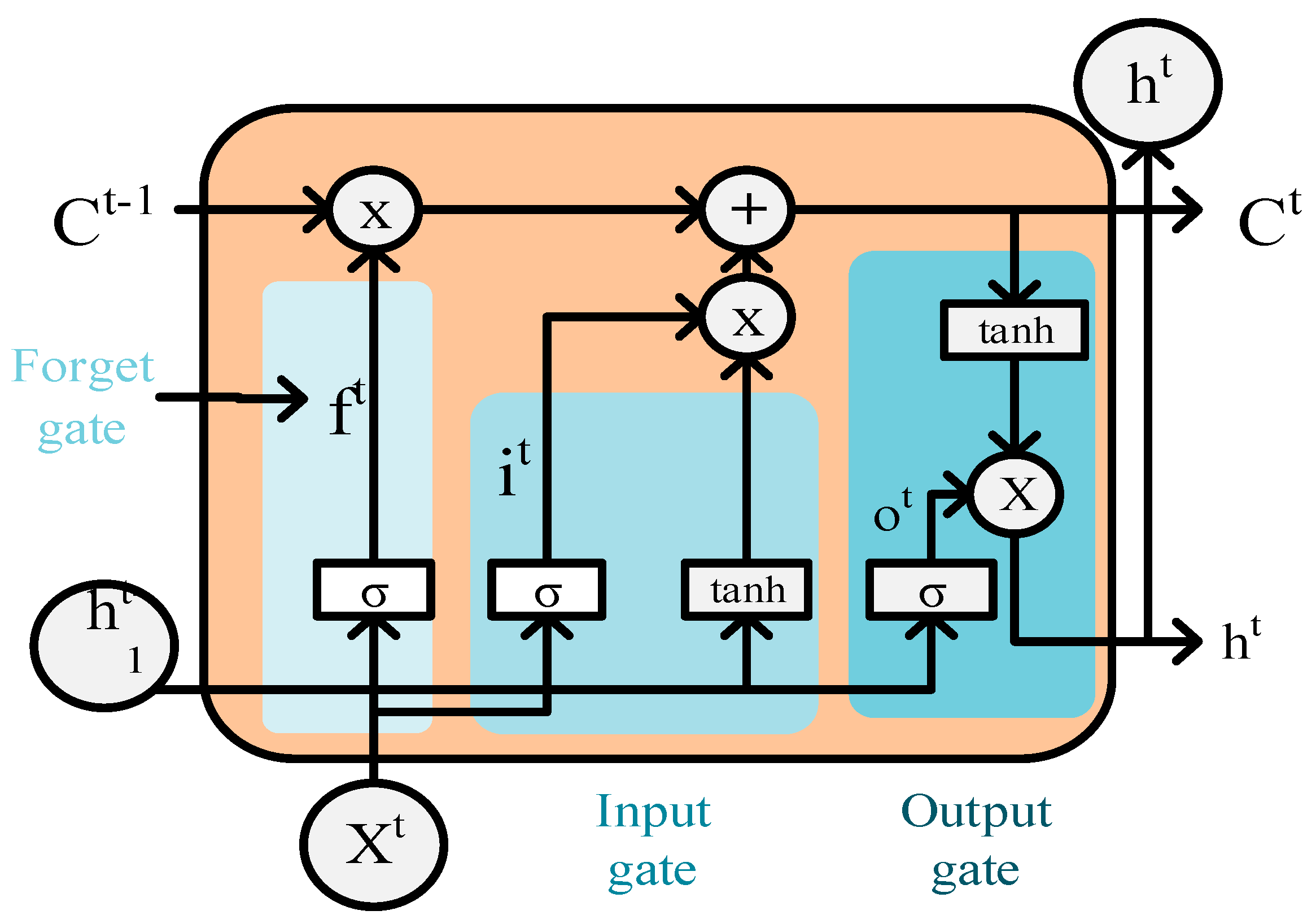
The Long Short-Term Memory (LSTM) neural network is a special type of recurrent neural network (RNN). It is primarily used for processing and predicting time series data. It addresses the issues of gradient vanishing and exploding that traditional RNNs face when dealing with long sequences. By designing a unique cell structure, LSTM can effectively remember long-term dependency information while ignoring irrelevant information. The structure of LSTM is shown in
Figure 2.
The core of the LSTM network is the cell state, which controls the flow of information through gating mechanisms. As shown in
Figure 2, it mainly consists of an input gate, a forget gate, and an output gate. The input gate updates the cell state primarily through the sigmoid activation function and tanh activation function layer, controlling whether the memory cell accepts the current information. This process is represented by Equations (7)–(9).
wherein
it is the output of the input gate.
is the sigmoid function shown in Equation (8).
W is the weight coefficient matrix.
x is the input vector.
b is the bias term.
is the output of the tanh functions shown in Equation (9),
is the output of the memory cell at the current time step, and
ht−1 is the output state of the neuron from the previous time step (
t − 1).
The value input to the forget gate is the current input and the previous hidden state. The function of the forget gate is to decide whether to retain or discard the information. This process can identify relevant feature information from the solar power output data and filter out irrelevant information, as shown in Equation (10).
wherein
ft is the output of the forget gate.
The previously input information is contained in the hidden state. The output gate determines what information to output as the value of the next hidden state, as expressed in Equation (11).
wherein
ot is the output of the output gate.
A traditional LSTM network can only predict the output at the current time step based on the information from previous time steps, thus only capturing unidirectional dependencies. In many tasks, the LSTM network may overlook crucial information from the future. The BiLSTM network can leverage both forward and backward context information. Thus, the current result is predicted not only from past states, but also from future states. Compared to LSTM, BiLSTM is more suitable for complex time series tasks involving long-term dependencies and asymmetric relationships. By capturing information from both ends of the sequence, the model accuracy is enhanced. The structure of the BiLSTM network is shown in
Figure 3.
The core idea of BiLSTM is to process the input data both forward and backward through two separate LSTM networks. As shown in
Figure 3, the update equations for BiLSTM network are given by Equation (12).
wherein
is the output of the forward LSTM,
is the output of the backward LSTM,
yt is the output of BiLSTM,
and
are output layer connection weight matrix, and
by is the bias vector of BiLSTM.
3.2. Genetic Algorithm
GA is a heuristic searching algorithm based on the principles of natural selection and genetics, aimed at finding approximate solutions to optimization problems in complex search spaces. It gradually optimizes candidate solutions by simulating mechanisms such as selection, crossover, and mutation from the biological evolution process. The advantage of the genetic algorithm lies in its strong global searching capability, helping to avoid local optima in complex multi-modal searching spaces. The computational process of GA for hyperparameter tuning is as follows.
(1) Population initialization
The initial population is a set of solutions (individuals) that is randomly generated. If an individual is represented by a binary string of length
L, and the population size is
N, the initialization process can be expressed as follows:
In the equation, represents the j-th gene of the i-th individual.
(2) Fitness evaluation
The hyperparameters are optimized by GA, and the mean squared error (MSE) of the validation data is calculated as the fitness value, as shown in Equation (14).
wherein
N is the number of samples in the validation set and
and
are the true values and predicted values of the validation set, respectively.
(3) Selection, crossover, mutation
The fitness value of each individual is calculated, and the population is sorted in ascending order of fitness values using the elitism selection strategy. The top 50% of individuals are then selected to pass on to the next generation.
The single-point crossover strategy is adopted for each hyperparameter (learning rate and number of neurons), as shown in Equation (15):
wherein
and
represent the gene values of offspring 1 and offspring 2 at the
i-th gene position, respectively.
and
represent the gene values of parent 1 and parent 2 at the
i-th gene position, respectively.
k is the randomly selected crossover point, satisfying
.
n is the gene sequence length of each individual.
A dynamic mutation rate is used for mutation procedure. The mutation rate decreases gradually as the number of generation increases, as shown in Equation (16):
wherein
β is the initial mutation rate,
η is the current mutation, and
g and
gs are the current generation of the population and the total number of generations, respectively. When a random number is smaller than the mutation rate, the number of neurons and the learning rate of the individual will be randomly regenerated.
(4) Repeat steps 2 and 3. After selection, crossover, and mutation operation, replace the old population with the new offspring individuals until the termination condition is met, i.e., the maximum number of iterations is reached.
Due to the relatively weak local searching capability of GA, it may suffer from premature convergence. As a result, combining GA optimization algorithms with stronger local searching capability can yield a more accurate population, accelerate convergence, and prevent premature convergence and entrapment in local optima.
3.3. Adaptive Multi-Objective Differential Evolution
The AMODE algorithm is a novel intelligent optimization algorithm [
31], primarily used for solving multi-objective optimization problems, especially two-objective optimization. It combines the multi-objective optimization and differential evolution (DE) strategies [
32], balancing global and local searching capabilities through adaptive mechanisms in the solution space. When dealing with two-objective optimization problems, the AMODE algorithm typically performs better in balancing convergence and solution diversity. For two-objective cases, the Pareto front is a two-dimensional curve. The algorithm can quickly find the distribution of solutions and effectively maintain diversity on the Pareto front. Additionally, the computational complexity is relatively low. The computational process of AMODE for hyperparameter tuning is as follows.
(1) Initialize the population and external archive
An initial population is randomly generated, with each individual representing a possible solution. Each individual is composed of multiple decision variables (genes). The external archive is used to store the non-dominated solutions (Pareto front) from the current population. The external archive can be initialized as an empty set or by filtering non-dominated solutions from the initial population and storing them. This archive is then used to maintain the solution archive and store Pareto optimal solutions during subsequent population updates. The population initialization is given by Equation (17).
wherein
Xi is the decision variables of the
i-th individual.
Xmin and
Xmax are the lower limit and upper limit of the decision variables.
is a randomly generated number uniformly distributed between [0, 1].
(2) Differential Evolution
DE is a population-based global optimization algorithm. It is commonly applied to function optimization problems in continuous spaces. Each individual is updated through mutation, crossover, and selection. These steps are repeated until the termination condition is satisfied.
The mutation step involves a linear combination of individuals in the current population. The mutant
Vi for each individual is generated by Equations (18) and (19).
wherein
Xr1,
Xr2, and
Xr3 are three different individuals randomly selected from the population.
F is the scaling factor used to control the magnitude of mutation.
The crossover operation recombines the genes of the mutant individual with the current individual, thereby generating more diverse candidate solutions. Binomial crossover is used for each dimension to decide whether to retain the gene of the current individual or the mutant. The calculation formulas are shown in Equations (20) and (21).
wherein
is the value of the test individual
Ui at the
j-th dimension.
is the value of the mutant
Vi at the
j-th dimension.
CR is the crossover probability, which is used to control the likelihood of inheriting genes from the mutant.
jrand is a randomly selected dimension that ensures that at least one dimension comes from the mutant
Vi.
The selection operation retains the superior solutions, gradually improving the overall quality of the population. A greedy selection strategy is used to choose the individual with better fitness, from the current individuals and the test individuals, to proceed to the next generation, as shown in Equation (22).
wherein
is the individual of a new generation.
and
are the objective function values of the test individual
Ui and the current individual
Xi, respectively.
dominates
indicates that the test individual
Ui is no worse than
Xi on all objectives and is better on at least one objective.
(3) Pareto Front Maintenance
The AMODE algorithm uses an external archive to store the currently found non-dominated solutions, and it updates it periodically. After each new candidate solution is generated, it is compared to the solutions in the external archive to determine whether it belongs to the Pareto front. If the new solution is not dominated by any solution in the external archive, it is added to the archive. Additionally, to maintain the diversity of Pareto front solutions, AMODE uses crowding distance calculation to measure the distribution of the solution set, as shown in Equation (23).
wherein
di is the crowding distance of individual
I.
is the value of individual
i on the
m-th objective.
and
are the maximum and minimum values of the
m-th objective, respectively.
If the number of solutions in the external archive exceeds the preset capacity limit, crowding distance is used for filtering. The solutions with larger crowding distances are removed. Ultimately, the solution set in the external archive represents the Pareto optimal set. These solutions are non-dominated, which cannot be outperformed by any other solutions across all objectives.
Owing to the DE and adaptive mechanisms, AMODE has strong local search capability. It enables more efficient exploration within the neighborhood of solutions. For example, in DE, the mutation operation generates new candidate solutions through weighted differences. As shown in Equation (18), when F is small, the newly generated candidate solutions are closer to the current solutions, thus achieving a fine local search. Additionally, AMODE adjusts the parameters of differential evolution through an adaptive mechanism, automatically balancing global and local search proportions at different search stages. It improves the chances of finding optimal solutions and avoiding missing local optima.
3.4. GA-AMODE-BiLSTM Model
A GA-AMODE based BiLSTM neural network model is established for short-term photovoltaic power output prediction. The process is illustrated in
Figure 4. The photovoltaic power forecasting consists of five steps as follows.
(1) Initialization and data preprocessing: According to the original photovoltaic power data, divide the training set, validation set, and test set, followed by data preprocessing operations. Initialize the parameters of the GA-AMODE algorithm and BiLSTM, including the population size of the GA, the maximum number of iterations, the maximum number of iterations for the AMODE algorithm, the initial mutation rate, the optimization ranges for the BiLSTM network’s learning rate, and the number of neurons in the hidden layer.
(2) Optimization of hyperparameters: The number of neurons and the learning rate of the BiLSTM neural network are the optimization objectives. GA-AMODE is used to find the optimal hyperparameters.
(3) Photovoltaic power forecasting: The optimal hyperparameters are used in BiLSTM. The model is trained on the training and validation sets after data preprocessing.
(4) Forecasting evaluation and statistical test: The forecasting results are compared to the true values. The indexes are calculated and the forecasting accuracy is evaluated. The model’s generalization ability is tested using a statistical test.
3.5. Model Evaluation and Statistical Testing
3.5.1. Evaluation Indexes
The prediction accuracy of the proposed model is evaluated using three indexes: R
2, RMSE, and MAE. The calculation formulas are given by Equations (24)–(26).
where
n is total number of samples.
3.5.2. Statistical Testing
To further evaluate the model’s stability and generalization ability and to better understand its real-world performance in practical applications, a T-test to compare mean differences and a KS-test to compare distribution differences are employed. Both methods are used to conduct statistical tests on the predicted and actual values of the model. The calculation formulas are shown in Equations (27)–(29) for the T-test and in Equations (30)–(31) for the KS-test.
wherein
is the average difference between the predicted values and the actual values. The
Sd is the standard deviation of the two datasets.
n is the sample size. After computing the T-statistic, the
p-value is obtained based on the degrees of freedom (
n−1). If the
p-value is less than 0.05 (commonly set as the significance level), it indicates a significant difference in means between the two datasets.
wherein
is the empirical distribution function of the predicted values.
is the empirical distribution function of the actual values.
D is the KS statistic, which represents the maximum absolute difference between the two empirical distribution functions at any point.
n is the sample size.
Xi represents the
i-th data point in the sample.
is an indicator function, where the value is 1 if
; otherwise, the value is 0.


