
Short-Term Electric Load Probability Forecasting Based on the BiGRU-GAM-GPR Model


Abstract
1. Introduction
2. Methods
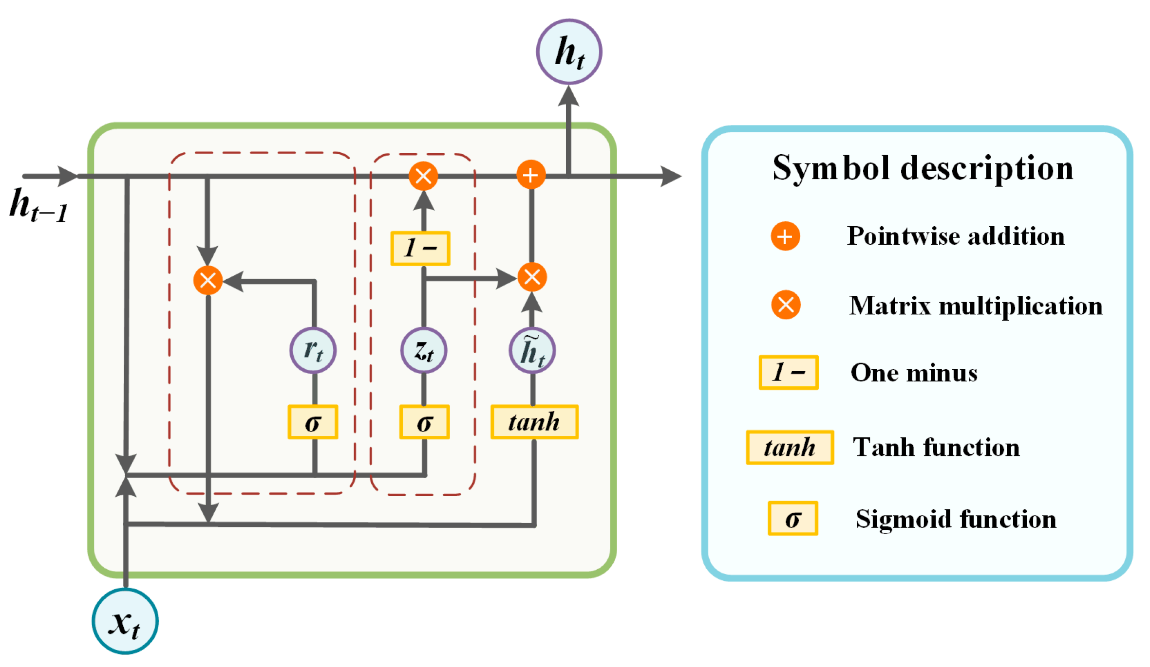
2.1. Bidirectional Gated Recurrent Unit (BiGRU)
2.2. Global Attention Mechanism (GAM)
2.3. Gaussian Process Regression (GPR)
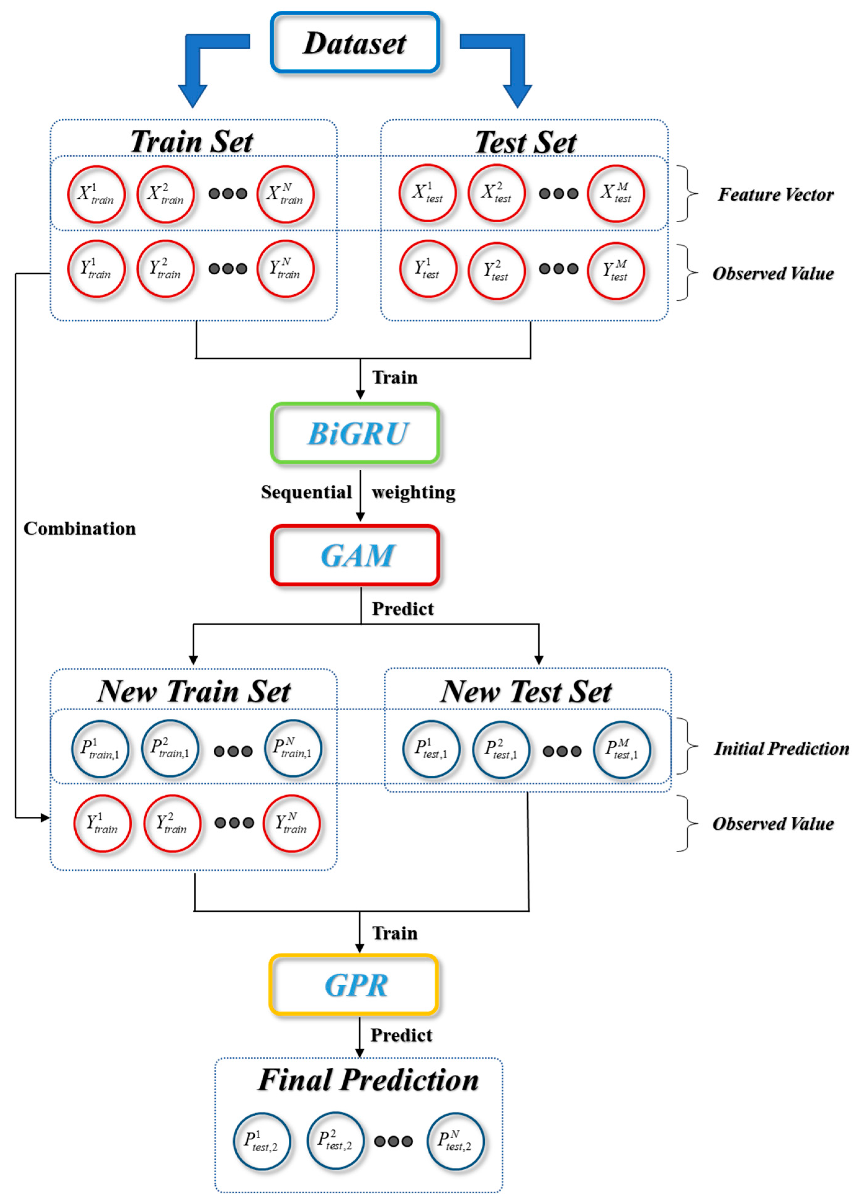
2.4. Load Forecasting Framework
2.5. Evaluation Metrics
2.5.1. Evaluation Metric of Point Prediction
2.5.2. Evaluation Metric of Probability Prediction
3. Case Study
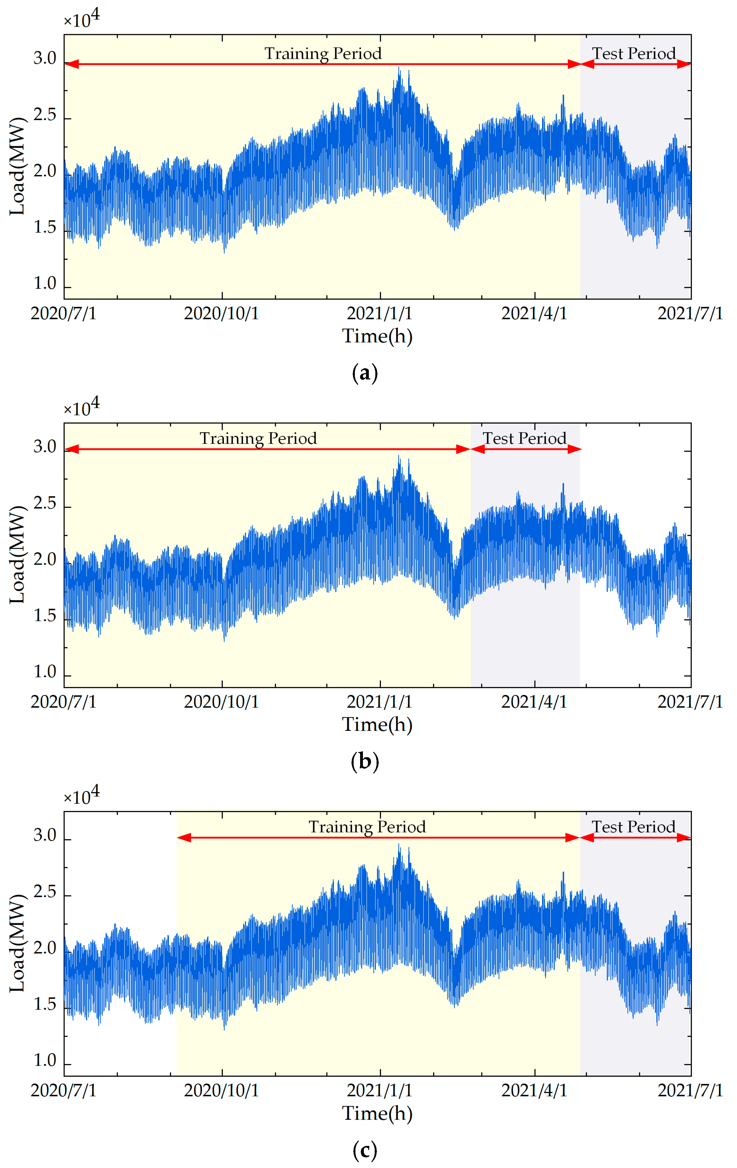
3.1. Study Data
3.2. Data Preprocessing
3.3. Comparative Experiment Design
4. Result
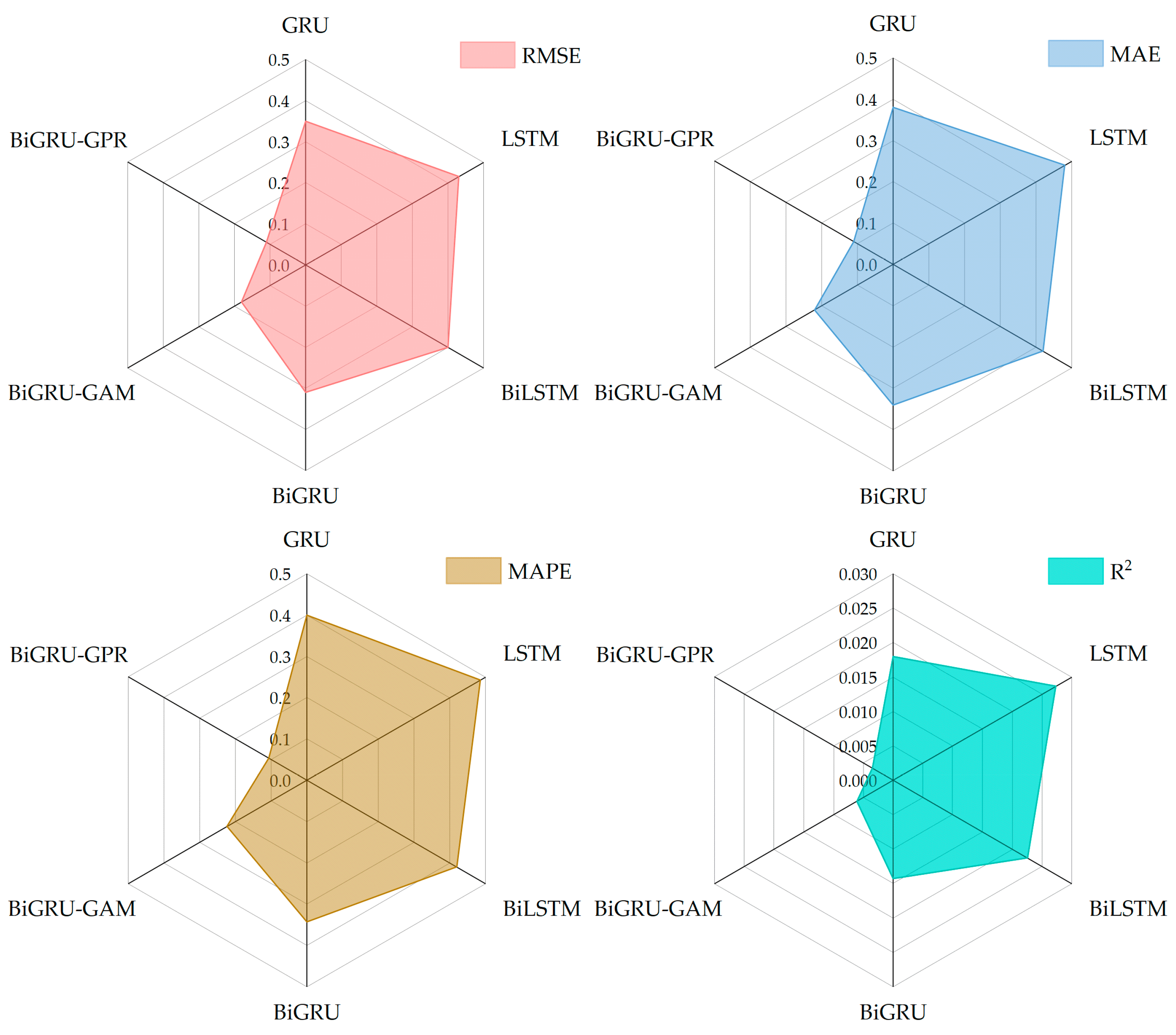
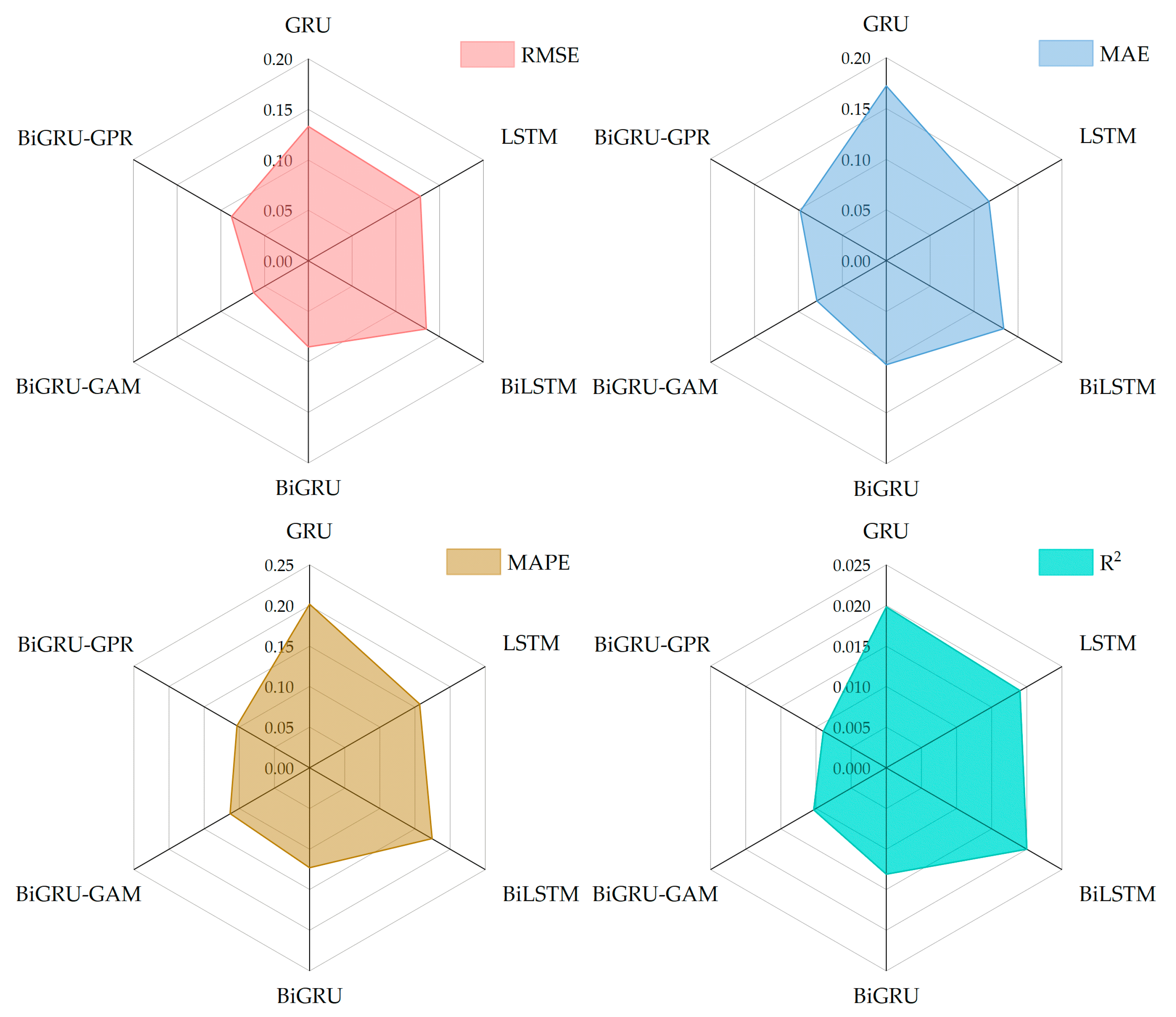
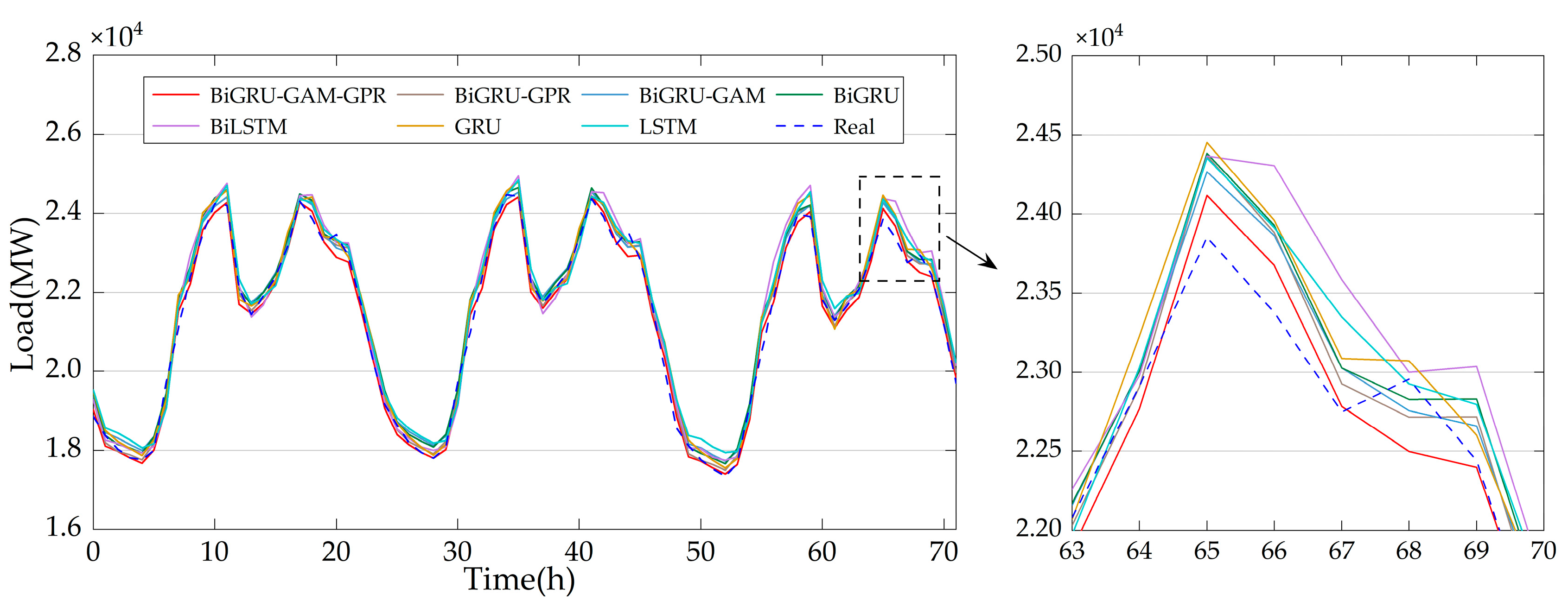
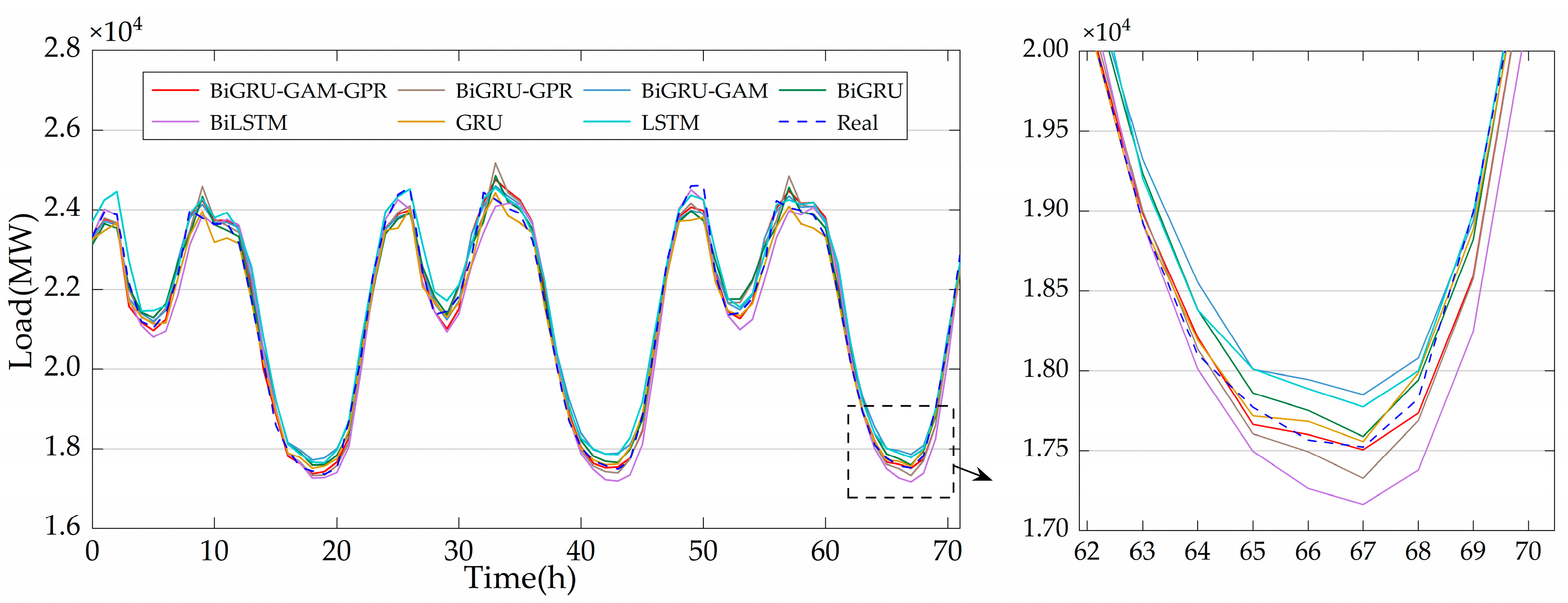
4.1. Deterministic Prediction Results
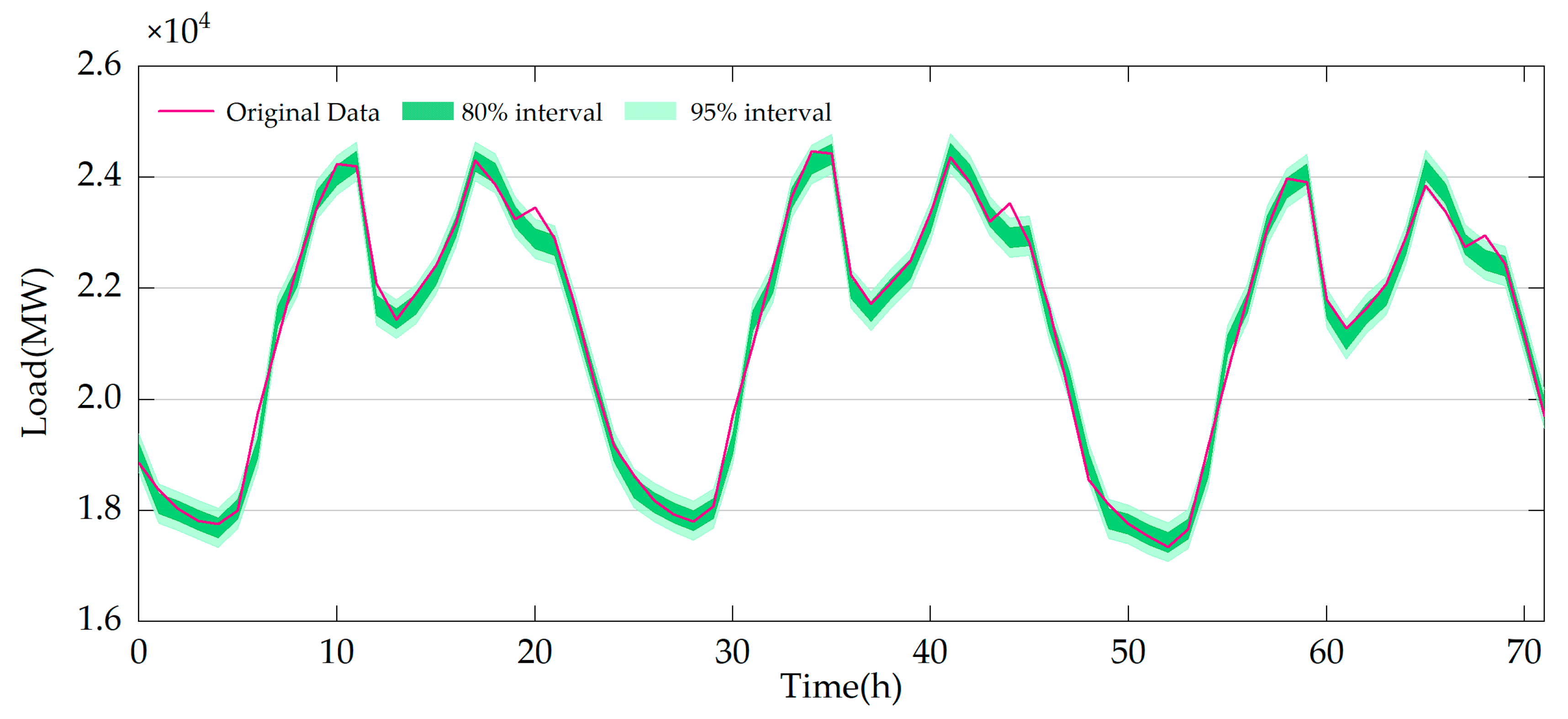
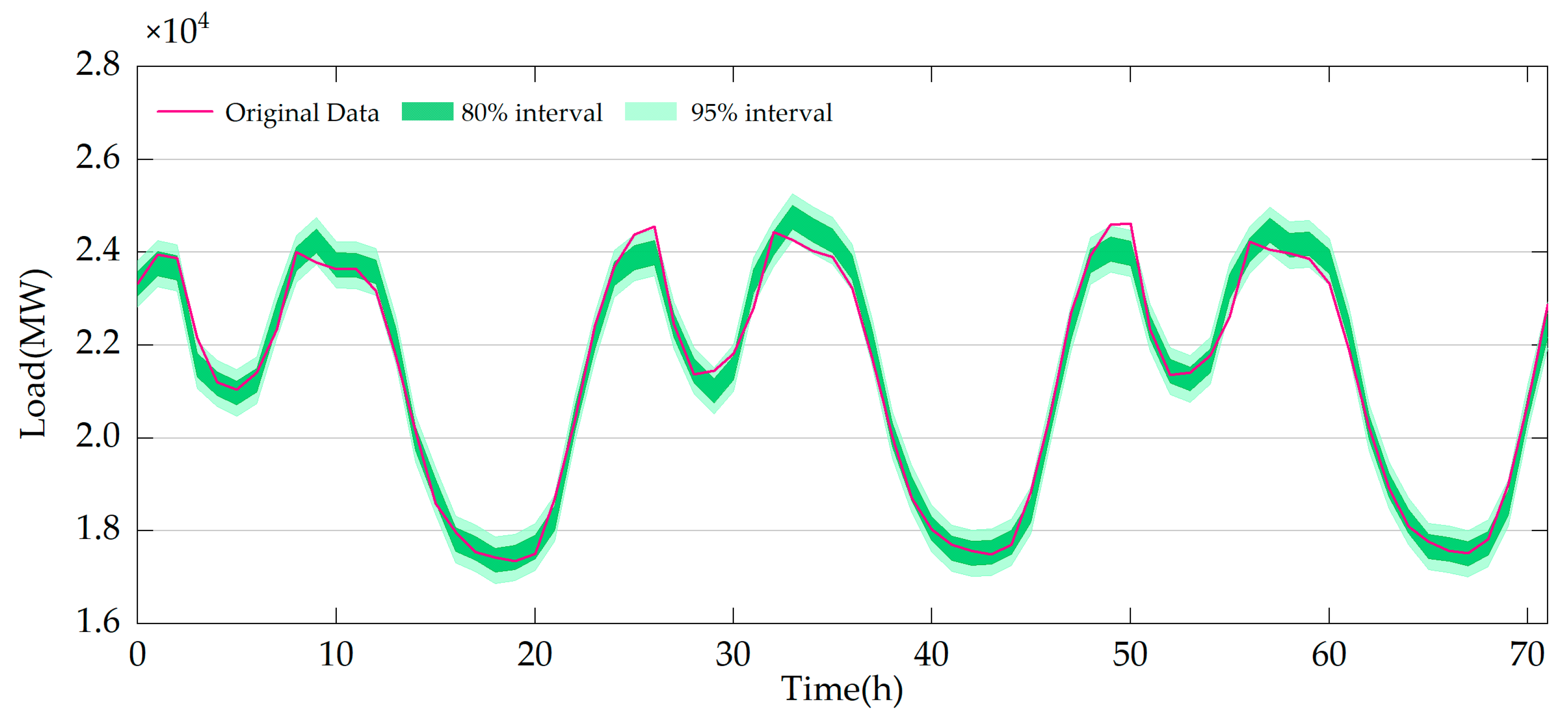
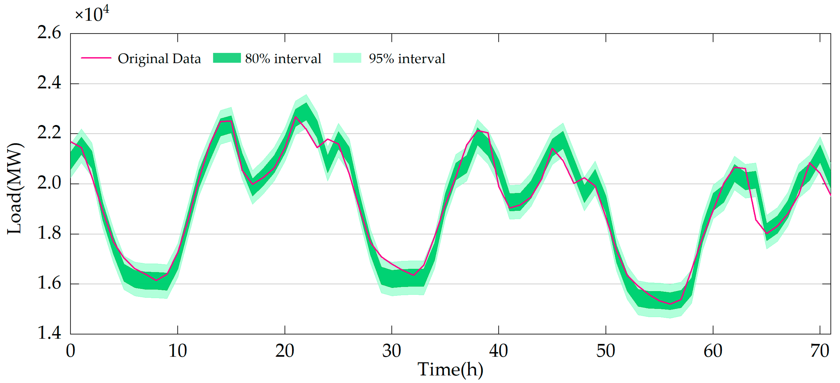
4.2. Probabilistic Prediction Results
5. Discussion
6. Conclusions
- (1)
- BiGRU demonstrates a strong capability of capturing the temporal dependencies within load time series, making it more suitable for addressing short-term load forecasting problems compared with other commonly used deep learning models.
- (2)
- By incorporating the global attention mechanism, the model is able to focus on the most important features within the sequence, thereby enhancing its ability to perceive spatial features in multi-feature sequences. This indicates that the global attention mechanism plays a positive role in improving the model’s prediction performance.
- (3)
- The GPR model further explores the intrinsic relationships within the data by extending deterministic prediction results to probabilistic outcomes. It adaptively fits the nonlinear relationships in the data, thereby avoiding overfitting and underfitting and reducing the impact of noise, which ultimately enhances the prediction performance.
- (4)
- The proposed BiGRU-GAM-GPR model demonstrates a superior performance in both deterministic and probabilistic predictions, thereby validating its practical value and robustness in short-term electricity load forecasting. This model provides guidance for the integration and grid connection of new energy sources as well as participation in market competition.
Author Contributions
Funding
Institutional Review Board Statement
Informed Consent Statement
Data Availability Statement
Conflicts of Interest
Abbreviations
| BiGRU | Bidirectional gated recurrent unit |
| GAM | Global attention mechanism |
| GPR | Gaussian process regression |
| GRU | Gated recurrent unit |
| LSTM | Long short-term memory |
| BiLSTM | Bidirectional long short-term memory |
References
- Abosedra, S.; Dah, A.; Ghosh, S. Electricity consumption and economic growth, the case of Lebanon. Appl. Energy 2009, 86, 429–432. [Google Scholar] [CrossRef]
- Adam, N.R.B.; Elahee, M.K.; Dauhoo, M.Z. Forecasting of peak electricity demand in Mauritius using the non-homogeneous Gompertz diffusion process. Energy 2011, 36, 6763–6769. [Google Scholar] [CrossRef]
- Ji, L.; Zhang, B.; Huang, G.; Xie, Y.; Niu, D. GHG-mitigation oriented and coal-consumption constrained inexact robust model for regional energy structure adjustment A case study for Jiangsu Province, China. Renew. Energy 2018, 123, 549–562. [Google Scholar] [CrossRef]
- Ruggles, T.H.; Dowling, J.A.; Lewis, N.S.; Caldeira, K. Opportunities for flexible electricity loads such as hydrogen production from curtailed generation. Adv. Appl. Energy 2021, 3, 100051. [Google Scholar] [CrossRef]
- He, W.; King, M.; Luo, X.; Dooner, M.; Li, D.; Wang, J. Technologies and economics of electric energy storages in power systems: Review and perspective. Adv. Appl. Energy 2021, 4, 100060. [Google Scholar] [CrossRef]
- Sabadini, F.; Madlener, R. The economic potential of grid defection of energy prosumer households in Germany. Adv. Appl. Energy 2021, 4, 100075. [Google Scholar] [CrossRef]
- He, F.; Zhou, J.; Feng, Z.; Liu, G.; Yang, Y. A hybrid short-term load forecasting model based on variational mode decomposition and long short-term memory networks considering relevant factors with Bayesian optimization algorithm. Appl. Energy 2019, 237, 103–116. [Google Scholar] [CrossRef]
- Zhang, X.; Wang, J.; Zhang, K. Short-term electric load forecasting based on singular spectrum analysis and support vector machine optimized by Cuckoo search algorithm. Electr. Power. Syst. Res. 2017, 146, 270–285. [Google Scholar] [CrossRef]
- Feng, C.; Wang, Y.; Chen, Q.; Ding, Y.; Strbac, G.; Kang, C. Smart grid encounters edge computing: Opportunities and applications. Adv. Appl. Energy 2021, 1, 100006. [Google Scholar] [CrossRef]
- Aslam, S.; Herodotou, H.; Mohsin, S.M.; Javaid, N.; Ashraf, N.; Aslam, S. A survey on deep learning methods for power load and renewable energy forecasting in smart microgrids. Renew. Sust. Energy Rev. 2021, 144, 110992. [Google Scholar] [CrossRef]
- Pramanik, A.S.; Sepasi, S.; Nguyen, T.; Roose, L. An ensemble-based approach for short-term load forecasting for buildings with high proportion of renewable energy sources. Energy Build. 2024, 308, 113996. [Google Scholar] [CrossRef]
- Waheed, W.; Xu, Q. Data-driven short term load forecasting with deep neural networks: Unlocking insights for sustainable energy management. Electr. Power Syst. Res. 2024, 232, 110376. [Google Scholar] [CrossRef]
- Yang, Z.; Ce, L.; Lian, L. Electricity price forecasting by a hybrid model, combining wavelet transform, ARMA and kernel-based extreme learning machine methods. Appl. Energy 2017, 190, 291–305. [Google Scholar] [CrossRef]
- de Oliveira, E.M.; Oliveira, F.L.C. Forecasting mid-long term electric energy consumption through bagging ARIMA and exponential smoothing methods. Energy 2018, 144, 776–788. [Google Scholar] [CrossRef]
- Li, J.; Deng, D.; Zhao, J.; Cai, D.; Hu, W.; Zhang, M.; Huang, Q. A Novel Hybrid Short-Term Load Forecasting Method of Smart Grid Using MLR and LSTM Neural Network. IEEE Trans. Ind. Inform. 2021, 17, 2443–2452. [Google Scholar] [CrossRef]
- Yang, D. On post-processing day-ahead NWP forecasts using Kalman filtering. Sol. Energy 2019, 182, 179–181. [Google Scholar] [CrossRef]
- Ye, J.; Dang, Y.; Yang, Y. Forecasting the multifactorial interval grey number sequences using grey relational model and GM (1, N) model based on effective information transformation. Soft Comput. 2020, 24, 5255–5269. [Google Scholar] [CrossRef]
- Qiu, X.; Suganthan, P.N.; Amaratunga, G.A.J. Ensemble incremental learning Random Vector Functional Link network for short-term electric load forecasting. Knowl-Based Syst. 2018, 145, 182–196. [Google Scholar] [CrossRef]
- Jain, R.; Mahajan, V. Load forecasting and risk assessment for energy market with renewable based distributed generation. Renew. Energy Focus 2022, 42, 190–205. [Google Scholar] [CrossRef]
- Chitsaz, H.; Shaker, H.; Zareipour, H.; Wood, D.; Amjady, N. Short-term electricity load forecasting of buildings in microgrids. Energy Build. 2015, 99, 50–60. [Google Scholar] [CrossRef]
- Hafeez, G.; Khan, I.; Jan, S.; Shah, I.A.; Khan, F.A.; Derhab, A. A novel hybrid load forecasting framework with intelligent feature engineering and optimization algorithm in smart grid. Appl. Energy 2021, 299, 117178. [Google Scholar] [CrossRef]
- Mughees, N.; Mohsin, S.A.; Mughees, A.; Mughees, A. Deep sequence to sequence Bi-LSTM neural networks for day-ahead peak load forecasting. Expert. Syst. Appl. 2021, 175, 114844. [Google Scholar] [CrossRef]
- Zhang, Z.; Hong, W.; Li, J. Electric Load Forecasting by Hybrid Self-Recurrent Support Vector Regression Model with Variational Mode Decomposition and Improved Cuckoo Search Algorithm. IEEE Access 2020, 8, 14642–14658. [Google Scholar] [CrossRef]
- Fan, G.; Han, Y.; Li, J.; Peng, L.; Yeh, Y.; Hong, W. A hybrid model for deep learning short-term power load forecasting based on feature extraction statistics techniques. Expert Syst. Appl. 2024, 238, 122012. [Google Scholar] [CrossRef]
- Wang, H.; Lei, Z.; Zhang, X.; Zhou, B.; Peng, J. A review of deep learning for renewable energy forecasting. Energy Convers. Manag. 2019, 198, 111799. [Google Scholar] [CrossRef]
- Kuster, C.; Rezgui, Y.; Mourshed, M. Electrical load forecasting models: A critical systematic review. Sustain. Cities Soc. 2017, 35, 257–270. [Google Scholar] [CrossRef]
- Behmiri, N.B.; Fezzi, C.; Ravazzolo, F. Incorporating air temperature into mid-term electricity load forecasting models using time-series regressions and neural networks. Energy 2023, 278, 127831. [Google Scholar] [CrossRef]
- Li, S.; Kong, X.; Yue, L.; Liu, C.; Khan, M.A.; Yang, Z.; Zhang, H. Short-term electrical load forecasting using hybrid model of manta ray foraging optimization and support vector regression. J. Clean. Prod. 2023, 388, 135856. [Google Scholar] [CrossRef]
- Aflaki, A.; Gitizadeh, M.; Kantarci, B. Accuracy improvement of electrical load forecasting against new cyber-attack architectures. Sustain. Cities Soc. 2022, 77, 103523. [Google Scholar] [CrossRef]
- Tarmanini, C.; Sarma, N.; Gezegin, C.; Ozgonenel, O. Short term load forecasting based on ARIMA and ANN approaches. Energy Rep. 2023, 9, 550–557. [Google Scholar] [CrossRef]
- Islam, B.U.; Ahmed, S.F. Short-Term Electrical Load Demand Forecasting Based on LSTM and RNN Deep Neural Networks. Math. Probl. Eng. 2022, 2022, 2316474. [Google Scholar] [CrossRef]
- Li, D.; Sun, G.; Miao, S.; Gu, Y.; Zhang, Y.; He, S. A short-term electric load forecast method based on improved sequence-to-sequence GRU with adaptive temporal dependence. Int. J. Electr. Power 2022, 137, 107627. [Google Scholar] [CrossRef]
- Xu, Y.; Jiang, X. Short-term power load forecasting based on BiGRU-Attention-SENet model. Energy Source Part A 2022, 44, 973–985. [Google Scholar] [CrossRef]
- Niu, D.; Yu, M.; Sun, L.; Gao, T.; Wang, K. Short-term multi-energy load forecasting for integrated energy systems based on CNN-BiGRU optimized by attention mechanism. Appl. Energy 2022, 313, 118801. [Google Scholar] [CrossRef]
- Li, X.L.; Wang, Y.Q.; Ma, G.B.; Chen, X.; Shen, Q.X.; Yang, B. Electric load forecasting based on Long-Short-Term-Memory network via simplex optimizer during COVID-19. Energy Rep. 2022, 8, 1–12. [Google Scholar] [CrossRef]
- Lin, Y.; Luo, H.; Wang, D.; Guo, H.; Zhu, K. An Ensemble Model Based on Machine Learning Methods and Data Preprocessing for Short-Term Electric Load Forecasting. Energies 2017, 10, 1186. [Google Scholar] [CrossRef]
- Wang, J.; Gao, J.; Wei, D. Electric load prediction based on a novel combined interval forecasting system. Appl. Energy 2022, 322, 119420. [Google Scholar] [CrossRef]
- Lin, W.; Wu, D.; Boulet, B. Spatial-Temporal Residential Short-Term Load Forecasting via Graph Neural Networks. IEEE Trans. Smart Grid 2021, 12, 5373–5384. [Google Scholar] [CrossRef]
- Zhu, B.; Zhang, Z.; Ma, T.; Yang, X.; Li, Y.; Shung, K.K.; Zhou, Q. (100)-Textured KNN-based thick film with enhanced piezoelectric property for intravascular ultrasound imaging. Appl. Phys. Lett. 2015, 106, 173504. [Google Scholar] [CrossRef]
- Feng, Y.; Shi, X.J.; Lu, X.Q.; Sun, W.; Liu, K.P.; Fei, Y.F. Predictions of friction and wear in ball bearings based on a 3D point contact mixed EHL model. Surf. Coat. Technol. 2025, 502, 131939. [Google Scholar] [CrossRef]
- Tan, M.; Liao, C.; Chen, J.; Cao, Y.; Wang, R.; Su, Y. A multi-task learning method for multi-energy load forecasting based on synthesis correlation analysis and load participation factor. Appl. Energy 2023, 343, 121177. [Google Scholar] [CrossRef]
- Zhu, H.; Lin, Q.; Li, X.; Xiao, H.; Shao, T. Short-term electrical load forecasting based on pattern label vector generation. Energ. Build. 2025, 331, 115383. [Google Scholar] [CrossRef]
- Xiao, W.; Mo, L.; Xu, Z.; Liu, C.; Zhang, Y. A hybrid electric load forecasting model based on decomposition considering fisher information. Appl. Energ. 2024, 364, 123149. [Google Scholar] [CrossRef]
- Huang, Q.; Li, J.; Zhu, M. An improved convolutional neural network with load range discretization for probabilistic load forecasting. Energy 2020, 203, 117902. [Google Scholar] [CrossRef]
- Lin, J.; Ma, J.; Zhu, J.; Cui, Y. Short-term load forecasting based on LSTM networks considering attention mechanism. Int. J. Electr. Power 2022, 137, 107818. [Google Scholar] [CrossRef]
- Bai, Y.; Xie, J.; Liu, C.; Tao, Y.; Zeng, B.; Li, C. Regression modeling for enterprise electricity consumption: A comparison of recurrent neural network and its variants. Int. J. Electr. Power 2021, 126, 106612. [Google Scholar] [CrossRef]
- Im, S.; Chan, K. Neural Machine Translation with CARU-Embedding Layer and CARU-Gated Attention Layer. Mathematics 2024, 12, 997. [Google Scholar] [CrossRef]
- Chorowski, J.; Bahdanau, D.; Serdyuk, D.; Cho, K.; Bengio, Y. Attention-Based Models for Speech Recognition. In Proceedings of the Advances in Neural Information Processing Systems 28: Annual Conference on Neural Information Processing Systems, Montreal, QC, Canada, 7–12 December 2015; p. 28. [Google Scholar]
- Zhang, Z.; Ye, L.; Qin, H.; Liu, Y.; Wang, C.; Yu, X.; Yin, X.; Li, J. Wind speed prediction method using Shared Weight Long Short-Term Memory Network and Gaussian Process Regression. Appl. Energy 2019, 247, 270–284. [Google Scholar] [CrossRef]
- Son, J.; Cha, J.; Kim, H.; Wi, Y. Day-Ahead Short-Term Load Forecasting for Holidays Based on Modification of Similar Days’ Load Profiles. IEEE Access 2022, 10, 17864–17880. [Google Scholar] [CrossRef]


| Study Case | Models | Hyperparameters |
|---|---|---|
| Case A | GRU | num layers = 2; hidden size = 64,128; learning rate = 0.001; batch size = 64; epoch = 100 |
| LSTM | num layers = 2; hidden size = 128,64; learning rate = 0.001; batch size = 64; epoch = 100 | |
| BiLSTM | Same as LSTM | |
| BiGRU | Same as GRU | |
| BiGRU-GAM | Same as GRU | |
| BiGRU-GPR | num layers = 2; hidden size = 64,128; learning rate = 0.001; batch size = 64; epoch = 100 | |
| BiGRU-GAM-GPR | num layers = 2; hidden size = 64,128; learning rate = 0.001; batch size = 64; epoch = 100 | |
| Case B | GRU | num layers = 2; hidden size = 64,128; learning rate = 0.001; batch size = 64; epoch = 100 |
| LSTM | num layers = 2; hidden size = 128,64; learning rate = 0.001; batch size = 64; epoch = 100 | |
| BiLSTM | Same as LSTM | |
| BiGRU | Same as GRU | |
| BiGRU-GAM | Same as GRU | |
| BiGRU-GPR | num layers = 2; hidden size = 64,128; learning rate = 0.001; batch size = 64; epoch = 100 | |
| BiGRU-GAM-GPR | num layers = 2; hidden size = 64,128; learning rate = 0.001; batch size = 64; epoch = 100 | |
| Case C | GRU | num layers = 2; hidden size = 64,128; learning rate = 0.001; batch size = 64; epoch = 100 |
| LSTM | num layers = 2; hidden size = 128,64; learning rate = 0.003; batch size = 64; epoch = 100 | |
| BiLSTM | Same as LSTM | |
| BiGRU | Same as GRU | |
| BiGRU-GAM | Same as GRU | |
| BiGRU-GPR | num layers = 2; hidden size = 64,128; learning rate = 0.001; batch size = 64; epoch = 100 | |
| BiGRU-GAM-GPR | num layers = 2; hidden size = 64,128; learning rate = 0.001; batch size = 64; epoch = 100 |
| Models | RMSE | MAE | MAPE | R2 |
|---|---|---|---|---|
| GRU | 458.86 | 388.36 | 2.00% | 0.9700 |
| LSTM | 521.30 | 457.76 | 2.35% | 0.9613 |
| BiLSTM | 491.12 | 409.38 | 2.09% | 0.9657 |
| BiGRU | 430.28 | 361.39 | 1.85% | 0.9736 |
| BiGRU-GAM | 360.90 | 305.36 | 1.56% | 0.9815 |
| BiGRU-GPR | 333.81 | 267.74 | 1.36% | 0.9841 |
| BiGRU-GAM-GPR | 296.29 | 239.44 | 1.21% | 0.9875 |
| Models | RMSE | MAE | MAPE | R2 |
|---|---|---|---|---|
| GRU | 520.27 | 403.84 | 1.75% | 0.9506 |
| LSTM | 460.72 | 357.14 | 1.59% | 0.9612 |
| BiLSTM | 510.02 | 408.32 | 1.86% | 0.9525 |
| BiGRU | 425.11 | 323.45 | 1.42% | 0.9670 |
| BiGRU-GAM | 407.62 | 341.90 | 1.56% | 0.9697 |
| BiGRU-GPR | 406.02 | 314.60 | 1.38% | 0.9698 |
| BiGRU-GAM-GPR | 394.27 | 305.79 | 1.34% | 0.9716 |
| Models | RMSE | MAE | MAPE | R2 |
|---|---|---|---|---|
| GRU | 605.74 | 519.50 | 2.81% | 0.9396 |
| LSTM | 602.01 | 486.94 | 2.66% | 0.9403 |
| BiLSTM | 606.78 | 496.49 | 2.72% | 0.9394 |
| BiGRU | 573.94 | 479.17 | 2.56% | 0.9458 |
| BiGRU-GAM | 560.13 | 467.04 | 2.53% | 0.9484 |
| BiGRU-GPR | 575.68 | 476.81 | 2.50% | 0.9497 |
| BiGRU-GAM-GPR | 525.06 | 430.15 | 2.24% | 0.9582 |
| Models | RMSE | MAE | MAPE | R2 |
|---|---|---|---|---|
| GRU | 35.43% | 38.35% | 39.51% | 1.80% |
| LSTM | 43.16% | 47.69% | 48.51% | 2.73% |
| BiLSTM | 39.67% | 41.51% | 42.07% | 2.26% |
| BiGRU | 31.14% | 33.74% | 34.34% | 1.43% |
| BiGRU-GAM | 17.90% | 21.59% | 22.38% | 0.61% |
| BiGRU-GPR | 11.24% | 10.57% | 10.63% | 0.35% |
| Models | RMSE | MAE | MAPE | R2 |
|---|---|---|---|---|
| GRU | 24.22% | 24.28% | 23.31% | 2.21% |
| LSTM | 14.42% | 14.38% | 15.58% | 1.08% |
| BiLSTM | 22.69% | 25.11% | 27.93% | 2.01% |
| BiGRU | 7.25% | 5.46% | 5.22% | 0.48% |
| BiGRU-GAM | 3.27% | 10.56% | 13.69% | 0.20% |
| BiGRU-GPR | 2.89% | 2.80% | 3.03% | 0.19% |
| Models | RMSE | MAE | MAPE | R2 |
|---|---|---|---|---|
| GRU | 13.32% | 17.20% | 20.14% | 1.98% |
| LSTM | 12.78% | 11.66% | 15.67% | 1.90% |
| BiLSTM | 13.47% | 13.36% | 17.45% | 2.00% |
| BiGRU | 8.52% | 10.23% | 12.29% | 1.31% |
| BiGRU-GAM | 6.26% | 7.90% | 11.32% | 1.03% |
| BiGRU-GPR | 8.79% | 9.79% | 10.32% | 0.90% |
| Index | Case A | Case B | Case C | ||||
|---|---|---|---|---|---|---|---|
| model | BiGRU-GPR | BiGRU-GAM-GPR | BiGRU-GPR | BiGRU-GAM-GPR | BiGRU-GPR | BiGRU-GAM-GPR | |
| CRPS | min | 151.128 | 135.791 | 219.621 | 213.776 | 236.609 | 253.609 |
| mean | 151.132 | 136.204 | 219.716 | 213.899 | 236.944 | 254.064 | |
| max | 151.138 | 136.337 | 219.760 | 213.959 | 237.043 | 254.694 | |
| PICP | min | 0.891 | 0.904 | 0.872 | 0.885 | 0.916 | 0.923 |
| mean | 0.891 | 0.904 | 0.873 | 0.885 | 0.917 | 0.925 | |
| max | 0.891 | 0.904 | 0.874 | 0.885 | 0.917 | 0.928 | |
| MPIW | 95%CL | 732.865 | 704.306 | 1023.779 | 1005.092 | 1197.047 | 1350.239 |
| 80%CL | 374.985 | 360.372 | 523.836 | 514.275 | 612.493 | 690.876 | |
Disclaimer/Publisher’s Note: The statements, opinions and data contained in all publications are solely those of the individual author(s) and contributor(s) and not of MDPI and/or the editor(s). MDPI and/or the editor(s) disclaim responsibility for any injury to people or property resulting from any ideas, methods, instructions or products referred to in the content. |
© 2025 by the authors. Licensee MDPI, Basel, Switzerland. This article is an open access article distributed under the terms and conditions of the Creative Commons Attribution (CC BY) license (https://creativecommons.org/licenses/by/4.0/).
Share and Cite
Shao, Q.; Bao, R.; Liu, S.; Fu, K.; Mo, L.; Xiao, W. Short-Term Electric Load Probability Forecasting Based on the BiGRU-GAM-GPR Model. Sustainability 2025, 17, 5267. https://doi.org/10.3390/su17125267
Shao Q, Bao R, Liu S, Fu K, Mo L, Xiao W. Short-Term Electric Load Probability Forecasting Based on the BiGRU-GAM-GPR Model. Sustainability. 2025; 17(12):5267. https://doi.org/10.3390/su17125267
Chicago/Turabian StyleShao, Qizhuan, Rungang Bao, Shuangquan Liu, Kaixiang Fu, Li Mo, and Wenjing Xiao. 2025. "Short-Term Electric Load Probability Forecasting Based on the BiGRU-GAM-GPR Model" Sustainability 17, no. 12: 5267. https://doi.org/10.3390/su17125267
APA StyleShao, Q., Bao, R., Liu, S., Fu, K., Mo, L., & Xiao, W. (2025). Short-Term Electric Load Probability Forecasting Based on the BiGRU-GAM-GPR Model. Sustainability, 17(12), 5267. https://doi.org/10.3390/su17125267