Income and Subjective Well-Being: The Importance of Index Choice for Sustainable Economic Development

Abstract

The relationship between income and subjective well-being (SWB) has been widely studied. While previous research has shown that the correlation between income and SWB is not always strong, there is limited research examining how the choice of SWB index influences this relationship. Drawing on survey data collected from 32 countries between 2015 and 2017, this study explores how the income–SWB relationship varies across different SWB indices. The dataset encompasses both developed and developing nations. We analyzed six types of SWB indices documented in the literature—covering a broader range than is typically included—and conducted comparative analyses. To account for the possibility of a nonlinear relationship between income and these SWB measures, we used a semiparametric approach by applying generalized additive models. Our findings show that these six indices can be categorized into three groups: (1) mental health and affect balance, (2) subjective happiness and eudaimonia, and (3) life satisfaction and the Cantril Ladder. These results underscore the significant impact that the selected SWB index can have on the income–SWB relationship. While economic development is often assumed to enhance SWB, our analysis reveals that this relationship does not hold consistently across all SWB indicators. In particular, certain indicators show little or no improvement in well-being despite increasing income levels, suggesting the presence of excessive or inefficient consumption that fails to contribute to genuine human flourishing. These findings challenge the conventional growth-centric paradigm and call for a deeper societal and academic inquiry into what constitutes “true prosperity.” From a sustainability perspective, aligning economic progress with authentic improvements in well-being is essential. This requires not only more careful selection and interpretation of SWB metrics, but also a broader re-evaluation of consumption patterns and policy goals to ensure that future development contributes meaningfully to human and ecological well-being.

1. Introduction

In recent decades, the intricate relationship between income and subjective well-being (SWB) has attracted considerable scholarly attention. Cross-sectional studies on income and SWB primarily seek to understand how SWB varies across different individuals. Kahneman and Deaton [1], for instance, used U.S. data to show that their measure of emotional well-being increased but plateaued at an annual income range of USD 60,000 to USD 90,000 when comparing different individuals. Conversely, Killingsworth [2], analyzing a similar U.S. dataset through an experience sampling study, found a linear relationship between SWB and the natural logarithm of income. This apparent discrepancy was clarified by Killingsworth et al. [3] in a collaborative reanalysis, which revealed that a plateau does indeed occur, but it is primarily observed among the least happy 20% of the population. OECD [4] reports that while higher income is generally associated with greater life satisfaction across its member countries, the marginal benefit of income declines as income increases, and emotional well-being is often less sensitive to income variation.

Jebb et al. [5] also provided noteworthy insights, reporting flattening patterns at around USD 95,000 for life evaluation and between USD 60,000 and USD 75,000 for emotional well-being. However, substantial regional disparities exist worldwide. In wealthier regions, these flattening patterns tend to emerge at higher income levels. Moreover, their research suggests that in some countries, income exceeding these flattening points correlates with reduced life evaluations, indicating differing ways in which individuals adapt to happiness and balance their fundamental needs against rising material aspirations.

The literature indicates that the association between income and SWB largely depends on which SWB measure is used. As Diener et al. [6] propose, the dynamics of this relationship can vary depending on whether the SWB measure is cognitively or affectively oriented. Measures focusing on cognitive aspects, such as life satisfaction, frequently show a positive correlation with income. In contrast, affective measures, such as subjective happiness, do not consistently exhibit this relationship.

Concerning cognitive measures, Stevenson and Wolfers [7] used data from over 140 countries and found no evidence of a strict “satiation point”—life satisfaction kept increasing with log income at both low and high income levels. Similarly, Deaton [8] used Gallup World Poll data and found a clear positive link between national income (log GDP) and average life satisfaction even among wealthy nations. At the same time, diminishing marginal returns are evident. Initial gains out of poverty have the largest impact on well-being. A common finding is that “absolute income matters more for the subjective well-being of people at low income levels” [9]. Once comfortable living standards are achieved, additional income contributes less to life satisfaction. Some researchers have attempted to identify a satiation point beyond which more income adds no further happiness. For instance, Jebb et al. [5] analyzed 1.7 million respondents worldwide and reported an average satiation income around USD 95,000 for life evaluations. Beyond that level, extra income yielded little or no increase in life satisfaction, and in some regions incomes above the satiation point were even associated with slight declines in life evaluation [5]. This pattern is interpreted as evidence of happiness adaptation: once material needs are met, rising aspirations and social comparisons may offset the effect of additional income [5]. Importantly, even when diminishing returns set in, the cross-sectional relationship between income and life satisfaction remains positive virtually everywhere: poverty is strongly associated with low life satisfaction, whereas more affluent groups report some of the highest scores [10,11]).

On the other hand, concerning affective measures, in poorer nations and for lower-income respondents, the emotional benefits of rising income are especially pronounced. Gaining additional income tends to reduce negative emotions like stress, anxiety, and sadness by alleviating material hardships [11]. Cross-country studies find that people in very poor countries experience less frequent enjoyment and more frequent pain or stress, on average, than those in richer countries [8]. Increasing income in those contexts can dramatically improve daily mood by providing food security, housing, and health care. By contrast, at higher income levels, further gains contribute relatively little to daily positive affect; other factors (such as social relationships, meaningful work, and time use) start to play a bigger role in day-to-day happiness [1,10]. There is even evidence that some negative affect measures might worsen at the top end of the income spectrum. A large-scale study of Americans found that beyond about USD 60,000–USD 75,000, higher incomes were associated with more daily stress, reversing the downward trend seen at lower incomes [2]. The author hypothesizes that at high income levels, stressors related to professional responsibilities, time pressures, or lifestyle may proliferate, partially counteracting the benefits of material comfort [2]. In summary, income strongly reduces negative affect and boosts positive affect up to moderate income levels. After basic needs and a middle-class standard are achieved, additional income yields only slight emotional rewards and may introduce new pressures. Life satisfaction, being a broad evaluation, continues to rise somewhat with income even when affective gains are minimal, underscoring the importance of distinguishing different SWB indicators in income research [1].

In this study, we emphasize comparing various SWB measures discussed in the literature. The ongoing debate around the income–SWB relationship may stem primarily from the differing measures of SWB employed. Our research focuses on cross-sectional comparisons that assess individuals’ well-being levels at a specific point in time relative to their incomes. The primary contribution of this study is its comprehensive comparison of a broader range of key SWB indicators commonly employed in previous research. Currently, there are few datasets that include comprehensive SWB indicators in a single questionnaire while also spanning a wide spectrum of economic development, from advanced economies to developing countries. We conducted an original survey covering 32 countries representing diverse stages of economic development.

This study aims to investigate the following research questions: (1) How does the relationship between income and SWB vary across different SWB indices? (2) Can SWB indices be categorized into distinct groups based on the nature of the income-SWB relationship? (3) What are the implications of these findings for policy and sustainable development?

The rest of this paper is structured as follows. Section 2 provides a comprehensive review of existing literature, highlighting distinctions among different SWB measures. In Section 3, we introduce our dataset and the estimation methodology. Section 4 presents the results of our estimations, and Section 5 offers a robustness check. Finally, Section 6 discusses these findings, outlines avenues for future research, and concludes the paper.

2. Literature on Differences Among SWB Measures

Many researchers distinguish between the cognitive and affective facets of SWB. For instance, Andrews and Withey [12] noted that enjoying activities and family life plays a more pronounced role in happiness than in life satisfaction. In contrast, factors such as financial stability, home ownership, and access to goods and services weigh more heavily on life satisfaction than on happiness. Similarly, Michalos [13] found that life satisfaction is more closely tied to various life domains, including health, financial security, and familial relationships. Veenhoven [14] further emphasized that the degree to which one’s income meets material needs has a stronger influence on life satisfaction than on happiness. Consequently, the prevailing literature suggests that income more substantially affects life satisfaction than subjective happiness. This distinction arises because life satisfaction involves evaluating whether one’s needs, ambitions, and aspirations are being met [12,15,16,17].

Diener et al. [18] defined life satisfaction as a “cognitive judgmental process dependent on a comparison of one’s circumstances with what is deemed an appropriate standard.” Similarly, the Cantril Ladder ([15]) is a well-known instrument for measuring life evaluation. Scholarly discourse often underscores the comparative nature of life evaluation, in which individuals assess their circumstances against various benchmarks. These benchmarks may include personal past experiences, comparisons with peers, global standards, or a dynamic “best possible life for you” criterion that shifts alongside improving living conditions [8]. Notably, the distinctions between metrics focused on life evaluation and those tied to emotional well-being likely stem from this inherently comparative element of life evaluation.

Kozma and Stones [19] proposed a theory suggesting that SWB depends on two distinct psychological states. The first involves a short-term state marked by affective experiences that respond to immediate environmental factors and encompass both positive and negative emotions. The second, by contrast, is a longer-term state related to affect but has a dispositional character, rendering it less susceptible to environmental fluctuations than the short-term state.

Parducci [20] and Kahneman [21] posited that SWB, over a given period, can be conceptualized as an aggregate of discrete hedonic values—encompassing both positive and negative dimensions of well-being—divided by the duration of that period. This perspective highlights the affective dimension of SWB, positioning it as a relatively short-term construct. In contrast, the broader evaluations people make when reflecting on their overall happiness represent a more cognitive approach. This cognitive viewpoint involves appraising significant components of one’s life. Consequently, distinguishing these short- and long-term perspectives can yield divergent findings regarding the relationship between income and SWB.

Peterson et al. [22] developed a comprehensive measure of happiness inspired by Seligman’s [23] theory of authentic happiness. Their instrument encompasses three core dimensions of happiness: hedonic well-being, life satisfaction, and eudaimonia. By accounting for both the experience of pleasure and the pursuit of a purpose-driven life, this framework offers a richer understanding of well-being.

Vitterso et al. [24] argue that hedonic and eudaimonic well-being are theoretically distinct, emphasizing that the foundational “cybernetic principles” governing hedonic well-being differ from those guiding eudaimonic well-being. Hedonic well-being centers on pleasure and positive affect, whereas eudaimonic well-being emphasizes living with purpose, contributing meaningfully to society, and adhering to moral values. This distinction highlights the multifaceted nature of human well-being. Sanjuan [25] investigated whether eudaimonic well-being influences life satisfaction through the mediating role of affect balance. The study’s findings suggest that eudaimonia is integral to well-being, enhancing life satisfaction by modulating the interplay of positive and negative emotions. In essence, these discussions underscore the importance of distinguishing eudaimonia from both life evaluation and the emotional dimensions of SWB, thereby reinforcing the multidimensionality of human well-being.

Moreover, various studies have juxtaposed mental health concepts with established SWB metrics. For example, Powdthavee and Van den Berg [26] incorporated the General Health Questionnaire (GHQ-12) alongside life satisfaction measures. Widely used in medical research, the GHQ-12 evaluates psychological stress and distress [27]. By focusing on well-being and specific emotional states at a given moment, this approach provides a more holistic understanding of SWB, underscoring the value of integrating mental health factors into SWB assessments.

Drawing on these scholarly contributions, the present study employs six key SWB measures: life satisfaction, the Cantril Ladder, subjective happiness, affect balance, mental health, and eudaimonia. Together, these indices offer a comprehensive perspective on individuals’ well-being, capturing both cognitive and affective elements as well as dimensions of mental health. This multi-pronged approach ensures a thorough evaluation of SWB.

3. Methods

We conducted an original survey in 32 countries from 2015 to 2017. The dataset includes the following countries: Australia, Sweden, Canada, the United States, the Netherlands, Germany, the United Kingdom, France, Japan, Italy, Spain, Greece, the Czech Republic, Poland, Chile, Venezuela, Russia, Malaysia, Brazil, Mexico, Romania, China, Colombia, Thailand, South Africa, Mongolia, Sri Lanka, the Philippines, Egypt, Vietnam, India, and Myanmar. Our combined sample encompasses both developed and developing nations.

For most countries, data were collected via online surveys. However, in countries where internet panels were not readily available (e.g., Vietnam, Kazakhstan, Mongolia, Sri Lanka, Egypt, and Myanmar), we employed a mixed-method approach. In Vietnam, for instance, we combined online and face-to-face surveys. By contrast, we conducted face-to-face surveys exclusively in Kazakhstan (Almaty), Mongolia (Ulaanbaatar), Sri Lanka (Colombo), Egypt (Cairo), and Myanmar (Yangon). The survey periods for each country are reported in

Table A1. Survey information.

Country *	Survey Period
Australia	10 February 2016	22 February 2016
Sweden	31 August 2016	12 September 2016
Canada	1 September 2016	13 September 2016
United States	16 August 2016	28 August 2016
Netherlands	29 August 2016	10 September 2016
Germany	26 August 2016	7 September 2016
United Kingdom	16 August 2016	28 August 2016
France	26 August 2016	7 September 2016
Japan	14 July 2015	5 August 2015
Italy	29 August 2016	10 September 2016
Spain	26 August 2016	7 September 2016
Greece	31 August 2016	12 September 2016
Czech Republic	8 March 2017	16 March 2017
Poland	8 March 2017	17 March 2017
Chile	24 July 2015	28 July 2015
Venezuela	24 July 2015	5 August 2015
Russia	31 August 2015	14 September 2015
Malaysia	23 July 2015	29 July 2015
Brazil	23 July 2015	26 July 2015
Mexico	24 July 2015	27 July 2015
Romania	8 March 2017	18 March 2017
China	12 January 2016	29 February 2016
Colombia	24 July 2015	27 July 2015
Thailand	18 July 2015	23 July 2015
South Africa	15 July 2015	23 July 2015
Mongolia	19 August 2015	3 September 2015
Sri Lanka	9 March 2017	30 March 2017
Philippines	15 July 2015	22 July 2015
Egypt	14 September 2015	27 October 2015
Vietnam	18 July 2015	28 July 2015
India	25 July 2015	11 August 2015
Myanmar	6 July 2015	10 August 2015

* Descending order by GNI per capita, calculated using the World Bank Atlas method (current USD) 2015.

in the Appendix A. We mainly used online surveys because it has the advantage of avoiding interviewer bias caused by arbitrary factors, such as the appearance or gender of interviewers, in response to sensitive questions, such as household income, employment, and marriage status [28].

Our selection of 32 countries was intended to capture a broad range of economic development stages. Nevertheless, data collection was constrained by the limited availability of internet panels at our research firm, Nikkei Research Inc., in Japan. The sample size for each country or city was primarily determined by its relative population share. We aligned sampling targets with each nation’s gender and age distribution. In cases where it was difficult to achieve target numbers in specific gender or age categories—particularly among women over 60 years of age in developing countries—we replaced those samples with participants from a closer age group. The survey questionnaire was designed to collect self-reported SWB (subjective well-being) levels, along with various personal and household characteristics. At the outset, respondents were informed about the purpose of the survey and their right to participate voluntarily; all respondents provided informed consent prior to participation.

The main objective of this study is to compare six major SWB indicators frequently employed in previous research. Currently, there are few datasets that include all six indicators in a single questionnaire while also spanning a wide spectrum of economic development, from advanced economies to developing countries. In light of this, and considering the aims of our study, our survey data can be considered unique. Additionally, our survey covers 32 countries representing diverse stages of economic development. Notably, in many of these countries, the number of respondents exceeds 1000. By comparison, the Gallup World Poll—one of the most prominent surveys on subjective well-being and the primary data source for the World Happiness Report—collects data from more countries but generally samples only 1000 respondents per country per year. Our survey, on the other hand, often includes a larger sample size per country.

We employ six distinct SWB measures in this study: life satisfaction, the Cantril Ladder, subjective happiness, affect balance, mental health, and eudaimonia. To account for the possibility of a nonlinear relationship between income and these SWB measures, we use a semiparametric approach by applying generalized additive models [29]. This analytical framework can be expressed as follows:

$${SWB}_i=C_1+f\left({income}_i\right)+\sum _j{\alpha }_j{X}_{ij}+{\delta }_z+{\tau }_t+ϵ$$

(1)

where i and z denote the individual and the country, respectively. ${SWB}_i$ corresponds to six types of SWB indexes that are standardized to fall between 0 and 1. ${income}_i$ denotes household income. We use absolute values of household income. $f\left(\right)$ is a generic, flexible functional form that allows for potentially nonlinear relationships. ${\alpha }_j$ represents coefficients, and $X_{ij}$ denotes the control variables for demographic factors such as gender, age, age squared, and marital status. Concerning age, previous studies find the so-called “U-shaped” relationship—where subjective well-being declines in midlife [30,31]. c₁ denotes the constant term, ${\delta }_z$ denotes the country-fixed effect, ${\tau }_t$ denotes the time-fixed effect, and $ϵ$ is the error term. Country-fixed effects are included to control for time-invariant national characteristics, such as economic development, cultural norms, and income inequality [32,33].

We utilized the R package “mgcv” for our analysis, applying iterative cubic spline smoothing to minimize partial residuals (i.e., residuals that remain after accounting for the effects of other variables in the model). When we use the loess function instead of the cubic spline function, we obtain nearly the same results. In this model, we select the smoothing parameters to optimize a prediction error using Generalized cross validation (GCV). Our estimation technique aligns with the approach described by Wood [34,35,36].

Table 1. Details of dependent and independent variables.

Variables	Survey Question	Notes
Life satisfaction	Overall, how satisfied are you with your life? Responses are given on an integer scale from 1 (not at all satisfied) to 5 (completely satisfied).	5: Completely satisfied, 1: Not at all satisfied; five-point scale (standardized into 0 to 1).
Cantril ladder	Imagine a ladder with steps numbered from 0 to 10 at the top. The top of the ladder represents the best possible life for you and the bottom of the ladder represents the worst possible life for you. On which step of the ladder would you say you personally feel that you stand at this time?	11-point scale, 10: Best possible life, 0: Worst possible life (standardized into 0 to 1)
Subjective happiness	Overall, how happy are you with your life? Responses are given on an integer scale from 1 (unhappy) to 5 (very happy).	5: Very happy, 1: unhappy, 5-point scale (standardized into 0 to 1).
Affect balance	How often have you felt or experienced the following feelings or actions? Please answer for number of times per week. Pleasure, Anger, Sadness, Enjoyment, Smile	3: Often, 2: Sometimes, 1: Rarely, 0: Not at all Affect balance = Average score of positive affect (Pleasure, Enjoyment, Smile)—Average score of negative affect (Anger, Sadness). Standardized into 0 to 1.
Mental health (12-item general health questionnaire (GHQ–12))	The response to each of the GHQ’s 12 questions is assigned a score based on a four-point Likert scale (from 0 to 3). The total score (between 0 and 36) is used as a measure of an individual’s mental health. The larger the score, the better the respondent’s mental health.	37 possible total scores ranging from 0 to 36 (standardized into 0 to 1).
Eudaimonia	Overall, to what extent do you feel that the things you do in your life are worthwhile? Responses are given on an integer scale from 0 (not at all worthwhile) to 10 (completely worthwhile).	11-point scale from 0 to 10 (standardized into 0 to 1).
Annual household income (USD)	Annual household income before tax (USD) Note: Nominal value	Each country’s currency unit is converted into USD using the annual exchange rate for 2015.
Age	Respondent’s age
Female dummy	Female dummy is coded 1 if the respondent is female, otherwise 0.
Marital dummy	Marital dummy is coded as 1 if the respondent answered married and does not distinguish whether the person was previously married.

provides variable descriptions, while

Table 2. Descriptive statistics for each SWB index and household income by country (Mean).

Country *	Sample Size	Life Satisfaction	Cantril Ladder	Subjective Happiness	Affect Balance	Mental Health	Eudaimonia	Annual Household Income (USD) (Average)	Annual Household Income (USD) (Median)
Australia	1727	0.707 (0.273)	0.680 (0.198)	0.732 (0.286)	0.617 (0.192)	0.638 (0.186)	0.721 (0.216)	56,011 (37,440)	0.707 (0.273)
Sweden	1115	0.740 (0.252)	0.688 (0.197)	0.741 (0.248)	0.611 (0.191)	0.648 (0.154)	0.699 (0.210)	51,956 (34,716)	0.740 (0.252)
Canada	1215	0.742 (0.256)	0.686 (0.194)	0.762 (0.262)	0.632 (0.186)	0.654 (0.165)	0.728 (0.211)	48,783 (34,278)	0.742 (0.256)
United States	10,173	0.747 (0.265)	0.695 (0.208)	0.768 (0.268)	0.622 (0.190)	0.646 (0.189)	0.751 (0.215)	60,126 (46,223)	0.747 (0.265)
Netherlands	1107	0.748 (0.237)	0.702 (0.164)	0.735 (0.242)	0.648 (0.184)	0.673 (0.169)	0.718 (0.173)	44,496 (32,122)	0.748 (0.237)
Germany	2754	0.703 (0.269)	0.665 (0.192)	0.708 (0.260)	0.645 (0.196)	0.641 (0.172)	0.708 (0.202)	45,488 (36,180)	0.703 (0.269)
United Kingdom	2667	0.698 (0.262)	0.656 (0.208)	0.712 (0.279)	0.615 (0.183)	0.624 (0.184)	0.699 (0.225)	57,251 (40,996)	0.698 (0.262)
France	1935	0.717 (0.266)	0.663 (0.181)	0.750 (0.248)	0.608 (0.197)	0.636 (0.153)	0.682 (0.190)	40,843 (32,963)	0.717 (0.266)
Japan	9784	0.589 (0.261)	0.593 (0.197)	0.657 (0.233)	0.604 (0.187)	0.638 (0.184)	0.627 (0.237)	50,899 (32,657)	0.589 (0.261)
Italy	1852	0.640 (0.241)	0.626 (0.181)	0.653 (0.233)	0.547 (0.201)	0.635 (0.135)	0.694 (0.183)	40,396 (30,730)	0.640 (0.241)
Spain	1934	0.732 (0.244)	0.667 (0.177)	0.737 (0.254)	0.600 (0.183)	0.663 (0.160)	0.753 (0.194)	37,365 (29,469)	0.732 (0.244)
Greece	1228	0.656 (0.259)	0.621 (0.188)	0.685 (0.237)	0.544 (0.197)	0.590 (0.178)	0.679 (0.184)	19,468 (15,567)	0.656 (0.259)
Czech Republic	1213	0.658 (0.208)	0.655 (0.182)	0.684 (0.189)	0.597 (0.161)	0.642 (0.154)	0.688 (0.178)	15,166 (13,023)	0.658 (0.208)
Poland	1816	0.685 (0.231)	0.637 (0.189)	0.699 (0.216)	0.607 (0.188)	0.631 (0.172)	0.711 (0.203)	16,821 (21,080)	0.685 (0.231)
Chile	1073	0.749 (0.233)	0.701 (0.171)	0.773 (0.215)	0.656 (0.177)	0.680 (0.171)	0.863 (0.171)	16,013 (14,205)	0.749 (0.233)
Venezuela	742	0.763 (0.254)	0.694 (0.208)	0.789 (0.219)	0.645 (0.193)	0.694 (0.168)	0.914 (0.165)	34,088 (34,087)	0.763 (0.254)
Russia	2133	0.604 (0.244)	0.597 (0.186)	0.685 (0.202)	0.586 (0.189)	0.640 (0.157)	0.666 (0.223)	11,531 (8693)	0.604 (0.244)
Malaysia	1032	0.649 (0.254)	0.648 (0.182)	0.710 (0.241)	0.620 (0.171)	0.649 (0.,176)	0.690 (0.191)	18,708 (13,424)	0.649 (0.254)
Brazil	2117	0.635 (0.257)	0.666 (0.192)	0.678 (0.235)	0.624 (0.175)	0.687 (0.186)	0.896 (0.176)	15,103 (14,267)	0.635 (0.257)
Mexico	1527	0.795 (0.208)	0.767 (0.155)	0.827 (0.189)	0.676 (0.170)	0.709 (0.156)	0.925 (0.136)	12,281 (11,730)	0.795 (0.208)
Romania	1217	0.708 (0.231)	0.700 (0.162)	0.730 (0.220)	0.608 (0.189)	0.653 (0.159)	0.759 (0.176)	15,799 (30,572)	0.708 (0.231)
China	19,877	0.719 (0.199)	0.676 (0.170)	0.711 (0.198)	0.692 (0.172)	0.726 (0.155)	0.725 (0.174)	20,357 (12,970)	0.719 (0.199)
Colombia	1035	0.812 (0.204)	0.739 (0.159)	0.825 (0.190)	0.664 (0.169)	0.724 (0.159)	0.933 (0.133)	10,833 (11,220)	0.812 (0.204)
Thailand	1096	0.697 (0.228)	0.663 (0.181)	0.700 (0.200)	0.651 (0.167)	0.691 (0.165)	0.805 (0.176)	17,744 (17,744)	0.697 (0.228)
South Africa	987	0.699 (0.259)	0.638 (0.193)	0.756 (0.268)	0.603 (0.186)	0.615 (0.198)	0.716 (0.199)	21,803 (20,913)	0.699 (0.259)
Mongolia	456	0.805 (0.243)	0.616 (0.189)	0.874 (0.193)	0.657 (0.183)	0.719 (0.130)	0.661 (0.220)	5403 (3271)	0.805 (0.243)
Sri Lanka	451	0.803 (0.184)	0.703 (0.181)	0.835 (0.165)	0.673 (0.186)	0.795 (0.129)	0.738 (0.182)	4121 (2046)	0.803 (0.184)
Philippines	1515	0.736 (0.228)	0.721 (0.159)	0.793 (0.211)	0.614 (0.155)	0.706 (0.162)	0.771 (0.162)	11,318 (15,058)	0.736 (0.228)
Egypt	569	0.730 (0.272)	0.615 (0.223)	0.711 (0.271)	0.596 (0.209)	0.715 (0.220)	0.671 (0.268)	5768 (5918)	0.730 (0.272)
Vietnam	1678	0.613 (0.255)	0.689 (0.162)	0.710 (0.238)	0.625 (0.163)	0.704 (0.158)	0.762 (0.163)	7995 (5900)	0.613 (0.255)
India	4833	0.782 (0.225)	0.723 (0.179)	0.795 (0.233)	0.610 (0.168)	0.689 (0.174)	0.746 (0.192)	14,158 (18,232)	0.782 (0.225)
Myanmar	1057	0.612 (0.172)	0.589 (0.150)	0.620 (0.169)	0.740 (0.126)	0.780 (0.094)	0.606 (0.155)	6602 (11,830)	0.612 (0.172)

Note: * Descending order by gross national income (GNI) per capita, calculated using the World Bank Atlas method (current USD, 2015). Standard deviations are in parentheses.

presents the sample sizes and summary statistics for each SWB index by country.

Table 3. Descripted statistics for control variables by country (Mean).

Country *	Sample Size	Age	Female Dummy	Marital Dummy
Australia	1727	46.327 (16.560)	0.510 (0.500)	0.527 (0.499)
Sweden	1115	47.994 (16.883)	0.522 (0.500)	0.367 (0.482)
Canada	1215	46.855 (16.367)	0.498 (0.500)	0.448 (0.497)
United States	10,173	46.178 (16.560)	0.510 (0.500)	0.527 (0.499)
Netherlands	1107	48.156 (16.546)	0.516 (0.500)	0.437 (0.496)
Germany	2754	48.613 (15.670)	0.500 (0.500)	0.423 (0.494)
United Kingdom	2667	47.009 (16.064)	0.499 (0.500)	0.462 (0.499)
France	1935	47.917 (15.754)	0.484 (0.500)	0.503 (0.500)
Japan	9784	49.776 (13.928)	0.555 (0.497)	0.691 (0.462)
Italy	1852	48.924 (15.001)	0.500 (0.500)	0.542 (0.498)
Spain	1934	46.782 (14.233)	0.493 (0.500)	0.530 (0.499)
Greece	1228	43.741 (11.652)	0.493 (0.500)	0.530 (0.499)
Czech Republic	1213	47.008 (16.006)	0.492 (0.500)	0.405 (0.491)
Poland	1816	46.094 (15.713)	0.490 (0.500)	0.519 (0.500)
Chile	1073	36.458 (12.917)	0.530 (0.499)	0.342 (0.475)
Venezuela	742	39.175 (12.437)	0.503 (0.500)	0.371 (0.484)
Russia	2133	42.017 (13.349)	0.460 (0.499)	0.246 (0.491)
Malaysia	1032	33.409 (10.214)	0.535 (0.499)	0.464 (0.499)
Brazil	2117	37.645 (12.962)	0.483 (0.500)	0.511 (0.500)
Mexico	1527	38.137 (13.822)	0.500 (0.500)	0.485 (0.500)
Romania	1217	47.134 (15.193)	0.493 (0.500)	0.579 (0.494)
China	19,877	41.150 (12.381)	0.506 (0.500)	0.754 (0.431)
Colombia	1035	37.927 (13.190)	0.485 (0.500)	0.384 (0.487)
Thailand	1096	38.103 (11.570)	0.519 (0.500)	0.501 (0.500)
South Africa	987	38.989 (13.467)	0.479 (0.500)	0.457 (0. 498)
Mongolia	456	39.434 (14.599)	0.465 (0.499)	0.689 (0.464)
Sri Lanka	451	42.293 (15.555)	0.475 (0.500)	0.816 (0.388)
Philippines	1515	37.232 (12.688)	0.486 (0.500)	0.442 (0.500)
Egypt	569	39.074 (12.884)	0.555 (0.497)	0.550 (0.498)
Vietnam	1678	31.817 (10.326)	0.521 (0.500)	0.569 (0.495)
India	4833	34.740 (11.761)	0.589 (0.492)	0.665 (0.472)
Myanmar	1057	38.710 (14.196)	0.460 (0.499)	0.580 (0.494)

* Descending order by GNI per capita, calculated using the World Bank Atlas method (current USD) 2015. Standard deviations are in parentheses.

displays the descriptive statistics for the control variables by country.

Concerning life satisfaction, previous studies have shown that single-item life satisfaction measures exhibit high validity, as they are strongly correlated with multi-item scales such as the Satisfaction With Life Scale (SWLS) and are predictive of related outcomes [37,38,39].

Subjective life evaluation was also measured using the Cantril Self-Anchoring Striving Scale ([15]), commonly referred to as the “Cantril ladder.” Participants were asked to imagine a ladder with steps from 0 (worst possible life) to 10 (best possible life) and indicate the step that best represents their life at the present moment. This measure is widely used in cross-national surveys such as the Gallup World Poll.

Eudaimonic well-being was assessed using a single-item measure: “Overall, to what extent do you feel the things you do in your life are worthwhile?” This item, used in OECD and the UK Office for National Statistics, has been shown to correlate strongly with multi-item measures of meaning in life and psychological well-being ([4,37,38].

Subjective happiness was measured using a single-item question, a method widely adopted in large-scale international surveys such as the World Values Survey, European Social Survey, and the Gallup World Poll. These surveys consistently employ a single, global question to assess individuals’ overall happiness, demonstrating its validity and practical utility in cross-national research [4,38].

To assess the internal consistency of the affect measures, we calculated Cronbach’s alpha separately for the positive and negative affect item sets. The positive affect dimension consisted of three items: Pleasure, Enjoyment, and Smile (Cronbach’s α = 0.82). The negative affect dimension included Anger and Sadness (Cronbach’s α = 0.75). As the affect balance score was computed as the difference between these two subscale means, internal consistency was not calculated for the composite score itself, in line with established psychometric recommendations [40,41].

Meanwhile, internal consistency of the mental health measure was assessed using Cronbach’s alpha for the 12-item General Health Questionnaire (GHQ–12). The GHQ–12 exhibited high internal consistency in our sample, with a Cronbach’s alpha of 0.88. This is consistent with previous studies that have reported alpha values ranging from 0.82 to 0.92 for the GHQ–12 in various populations [42,43].

4. Results

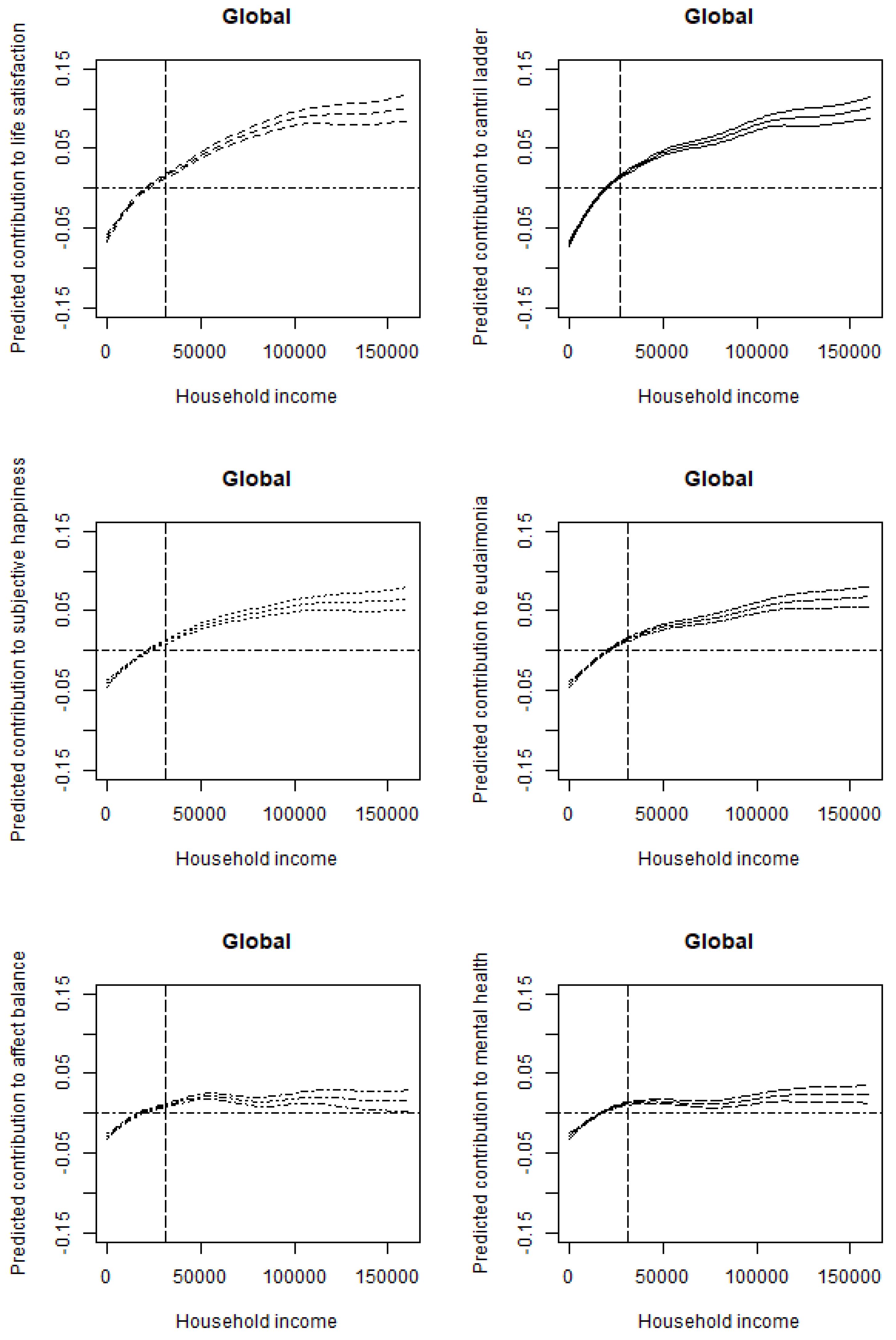
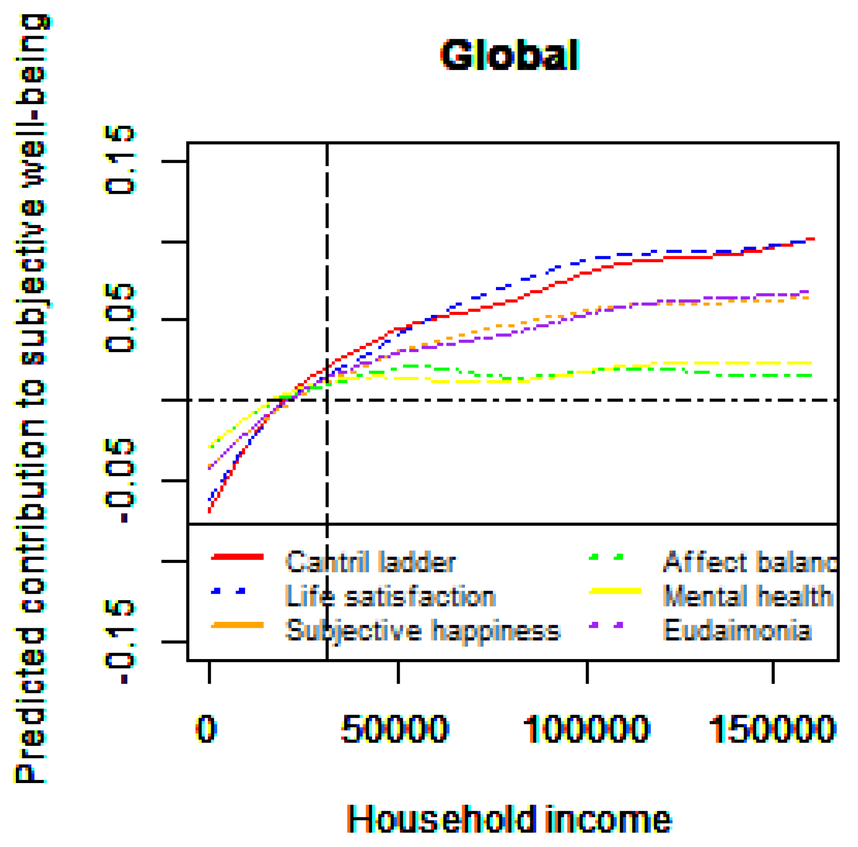
Figure 1 and Figure 2 illustrate the estimated relationship between income and SWB for the combined sample of all countries. Specifically, Figure 1 shows the predicted relationships between income and the six SWB indices, whereas Figure 2 provides individual income–SWB curves for each index, along with the associated 95% confidence intervals. The estimated results for the parametric terms, as well as model fit statistics—including approximate significance of the smooth terms (F-values), Generalized cross validation (GCV), and adjusted R-squared—are presented in

Table 4. Estimated results.

	Model A	Model B	Model C	Model D	Model E	Model F
	Life satisfaction	Cantril ladder	Subjective happiness	Eudaimonia	Affect balance	Mental health
Female dummy	1.27 × 10−2 *** (7.66)	2.33 × 10−2 *** (18.30)	1.79 × 10−2 *** (11.15)	1.70 × 10−2 *** (12.30)	3.31 × 10−2 * (2.57)	−8.78 × 10−2 *** (−7.39)
Age	−9.70 × 10−3 *** (−27.41)	−5.71 × 10−3 *** (−21.07)	−9.26 × 10−3 *** (−27.13)	−5.58 × 10−3 *** (−19.00)	−4.15 × 10−3 *** (−15.12)	−3.50 × 10−3 *** (−13.83)
Age squared	1.09 × 10−4 *** (28.25)	6.82 × 10−5 *** (22.99)	1.01 × 10−4 *** (27.00)	6.89 × 10−5 *** (21.46)	5.74 × 10−5 *** (19.10)	5.30 × 10−5 *** (19.15)
Marital dummy	6.54 × 10−2 *** (33.29)	4.89 × 10−2 *** (32.44)	7.57 × 10−2 *** (39.87)	4.45 × 10−2 *** (27.25)	2.73 × 10−2 *** (17.85)	2.31 × 10−2 *** (16.38)
Constant term	6.72 × 10−1 *** (87.60)	6.06 × 10−1 *** (103.13)	7.42 × 10−1 *** (100.21)	6.39 × 10−1 *** (100.47)	6.13 × 10−1 *** (102.99)	6.31 × 10−1 *** (114.87)
Approximate significance of smooth terms (F values)	330.2 ***	470.1 ***	243.0 ***	269.9 ***	139.1 ***	160.7 ***
Generalized cross validation (GCV)	34.43	34.35	35.75	34.75	33.32	32.15
Adjusted R squared	0.135	0.133	0.104	0.166	0.092	0.119
Time-fixed effects	Yes	Yes	Yes	Yes	Yes	Yes
Country-fixed effects	Yes	Yes	Yes	Yes	Yes	Yes
Observations	83,915	83,915	83,915	83,915	83,915	83,915

Note: Values in parentheses are t-values. * and *** indicate “significant” at the 10% level and the 1% level, respectively.

. The approximate significance of the smooth terms confirms that all nonparametric functions depicted in Figure 1 and Figure 2 are statistically significant. With regard to the control variables, most of our results align with previous literature.

As shown in Figure 1 and Figure 2, all SWB indices exhibit generally positive but diminishing slopes, with a pronounced decline in slope around the USD 20,000 income level. Notably, affect balance and mental health show considerably smaller slopes compared with life satisfaction, the Cantril Ladder, subjective happiness, and eudaimonia.

Furthermore, when we group the six SWB indices into three categories—(1) affect balance and mental health, (2) subjective happiness and eudaimonia, and (3) life satisfaction and the Cantril Ladder—we observe that the 95% confidence intervals do not overlap between these groups, although overlaps do occur within each group. Nevertheless, some within-group variations emerge. In group (1), for instance, the predicted slope for affect balance flattens at approximately USD 75,000, whereas mental health does not exhibit the same pattern. In group (2), although the confidence intervals overlap, the predicted contribution to life satisfaction tends to exceed that of the Cantril Ladder. Finally, within group (3), subjective happiness shows a greater predicted contribution than eudaimonia.

5. Robustness

5.1. Robustness: Additional Control Variables

The literature endeavors to clarify what the income variable represents. Economic development can influence SWB both positively and negatively [44]. As economies grow, increased tax revenue may lead to improved health care systems, greater access to medical services, and higher-quality food, all of which contribute to better overall health. Health is one of the most significant determinants of SWB [45].

Moreover, Putnam [46] demonstrates that in eight developed countries experiencing rising income levels, social capital has declined, which could adversely affect individual SWB. Other studies similarly find that social capital has a substantial positive impact on SWB [47].

Additionally, economic development may be accompanied by long working hours, which can negatively affect individual SWB. Research indicates that extended work hours reduce SWB (e.g., [48,49]).

Furthermore, as economies develop, the living environment can also influence individual SWB. Studies show that air pollution ([50,51,52,53,54,55,56,57,58,59]) and greenery ([60,61,62,63,64]) can affect individual SWB. Safety also plays a role in SWB [65,66]. Within a given country, individual-level estimations suggest that people’s residential choices, shaped by their income levels, are a critical determinant of environmental pollution, greenery, and safety—all of which, in turn, influence SWB. Future research should address potential spurious correlations related to income.

Consequently, for the robustness check, we included these factors as additional control variables. It is worth noting that the income–SWB relationship may be influenced not only by demographic variables but also by social factors.

Table 5. Additional control variables.

Variables	Survey Question	Notes
Subjective health	All in all, how would you describe your state of health?	5: Very good, 4: Good, 3: Neither, 2: Poor, 1: Very poor, five-point scale.
Social capital	Please select all items that you feel important in your life. From items that you have chosen to be important in your life, please select all items that you are satisfied with. A: Relationship with family B: Relationship with friends and acquaintances	1: the respondent chooses both A and B. 0.5: the respondent chooses either A or B. 0: the respondent chooses neither A nor B.
Working hours	Please tell us about your average working day. Please select average hours that you spend on working (including housework) or school hours.	Unit: hour 0: 0 h 0.15: Less than 15 min 0.3: 15 min to less than 30 min 0.75: 30 min to less than 1 h 1.5: 1 h to less than 2 h 2.5: 2 h to less than 3 h 3.5: 3 h to less than 4 h 4.5: 4 h to less than 5 h 5.5: 5 h to less than 6 h 6.5: 6 h to less than 7 h 7.5: 7 h to less than 8 h 8.5: 8 h to less than 9 h 9.5: 9 h to less than 10 h 10.5: 10 h to less than 11 h 11.5: 11 h to less than 12 h 12.5: 12 h or more
Environment	Now we will ask about your living environment. Please select all items that you are dissatisfied with. A: Landscape/Scenery B: Air pollution C: Quality of domestic water D: Surrounding green	1: all items selected 0.75: three items selected 0.5: two items selected 0.25: one items selected 0: no item selected
Safety	Please tell us about the safety of your neighborhood.	4: Very safe, 3: Moderately safe, 2: Slightly dangerous, 1: Very dangerous, four-point scale.

presents detailed information about these additional control variables.

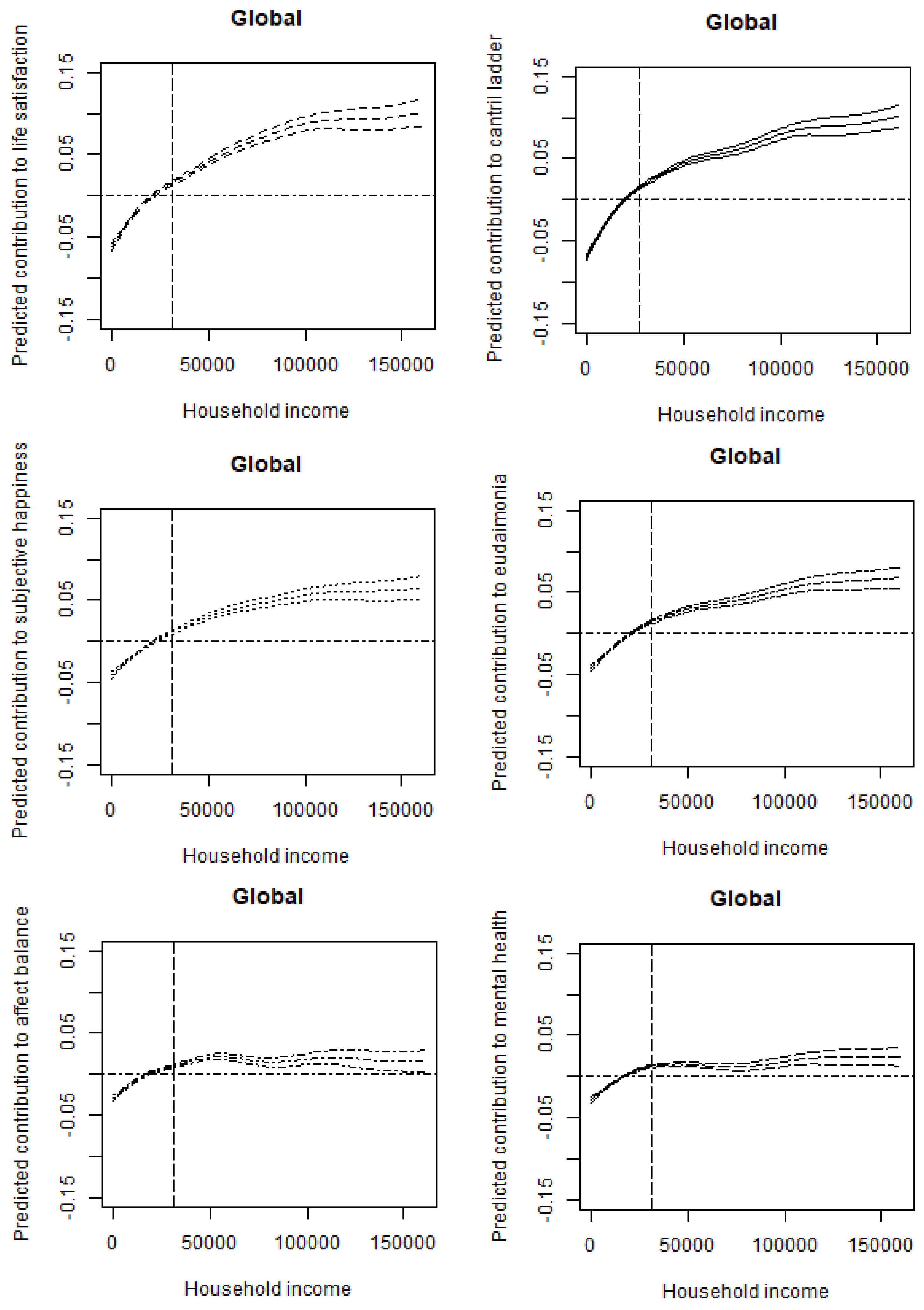
Figure 3 and Figure 4 illustrate the estimated relationship between income and SWB, incorporating additional control variables.

Table 6. Estimated results (including additional control variables).

	Model G	Model H	Model I	Model J	Model K	Model L
	Life satisfaction	Cantril ladder	Subjective happiness	Eudaimonia	Affect balance	Mental health
Female dummy	9.14 × 10−3 *** (6.01)	1.99 × 10−2 *** (17.03)	1.51 × 10−2 *** (10.38)	1.57 × 10−2 *** (12.23)	3.69 × 10−3 *** (3.09)	−1.05 × 10−3 *** (−9.85)
Age	−5.82 × 10−3 *** (−17.88)	−2.67 × 10−3 *** (−10.66)	−5.49 × 10−3 *** (−17.67)	−2.89 × 10−3 *** (−10.53)	−1.95 × 10−3 *** (−7.63)	−7.09 × 10−4 ** (−3.10)
Age squared	7.24 × 10−5 *** (20.16)	3.87 × 10−5 *** (14.02)	6.51 × 10−5 *** (18.98)	4.42 × 10−5 *** (14.59)	3.78 × 10−5 *** (13.41)	2.67 × 10−5 *** (10.60)
Marital dummy	4.44 × 10−2 *** (24.84)	3.30 × 10−2 *** (23.98)	5.40 × 10−2 *** (31.60)	2.80 × 10−2 *** (18.59)	1.16 × 10−2 *** (8.25)	6.86 × 10−2 *** (5.47)
Subjective health	9.21 × 10−2 *** (99.09)	6.90 × 10−2 *** (96.56)	8.88 × 10−2 *** (99.96)	6.77 × 10−2 *** (86.37)	5.66 × 10−2 *** (77.54)	3.27 × 10−2 *** (42.68)
Social capital	8.37 × 10−2 *** (34.60)	6.32 × 10−2 *** (33.98)	1.05 × 10−1 *** (45.51)	8.41 × 10−2 *** (41.22)	1.11 × 10−2 *** (58.15)	7.15 × 10−2 *** (42.09)
Working hours	−1.68 × 10−3 *** (−6.93)	−1.76 × 10−3 *** (−9.43)	−8.60 × 10−4 *** (−3.71)	1.10 × 10−3 (0.536)	1.74 × 10−3 *** (9.10)	−4.09 × 10−3 * (−2.40)
Environment	−6.04 × 10−2 *** (−22.42)	−5.66 × 10−2 *** (−27.30)	−4.50 × 10−2 *** (−17.47)	−2.47 × 10−2 *** (−10.87)	−7.89 × 10−3 *** (−3.73)	−4.05 × 10−2 *** (−21.39)
safety	3.46 × 10−2 *** (31.76)	2.45 × 10−2 *** (29.22)	3.76 × 10−2 *** (36.07)	2.81 × 10−2 *** (30.53)	2.73 × 10−2 *** (31.87)	3.27 × 10−2 *** (42.68)
Constant term	1.66 × 10−1 *** (20.563)	2.32 × 10−1 *** (37.27)	2.28 × 10−1 *** (29.51)	2.46 × 10−1 *** (36.09)	2.49 × 10−1 *** (39.23)	2.34 × 10−1 *** (41.10)
Approximate significance of smooth terms (F values)	191.1 ***	312.7 ***	115.3 ***	136.1 ***	44.1 ***	54.32 ***
Generalized cross validation (GCV)	34.25	34.56	35.85	34.46	33.75	32.64
Adjusted R squared	0.295	0.288	0.285	0.299	0.242	0.309
Time-fixed effects	Yes	Yes	Yes	Yes	Yes	Yes
Country-fixed effects	Yes	Yes	Yes	Yes	Yes	Yes
Observations	83,915	83,915	83,915	83,915	83,915	83,915

Note: Values in parentheses are t-values. *, ** and *** indicate “significant” at the 10% level, 5% level and the 1% level, respectively.

presents the estimated results for the parametric terms, along with model fit statistics such as the approximate significance of the smooth terms (F-values) and adjusted R-squared. The significance of these smooth terms confirms that all nonparametric functions shown in Figure 3 and Figure 4 are statistically significant. The inclusion of additional control variables substantially increased the adjusted R-squared values. Concerning the control variables, most of our findings align with previous studies. However, similar to the results in Table 4, an unexpected outcome appears in Model L, where the female dummy variable exhibits a negative sign, contrary to our expectations. Additionally, in Model J, the coefficient for working hours is statistically insignificant, whereas in Model K, it is both statistically significant and positively signed.

Overall, these results are consistent with those illustrated in Figure 1 and Figure 2. Once again, the six SWB indices can be categorized into three groups: (1) affect balance and mental health, (2) subjective happiness and eudaimonia, and (3) life satisfaction and the Cantril Ladder. Although the confidence intervals do not overlap across groups, they do overlap within each group. Notably, the predicted contributions to SWB are smaller than those observed in Figure 1 and Figure 2.

5.2. Robustness: Sub-Samples

Our study converts household income into (USD in nominal terms using 2015 exchange rates). Our methodological choice may limit the cross-national comparability of the income variable, especially between developed and developing countries, where USD 1 in nominal terms can have vastly different purchasing power. We thus examine the association between income and six SWB indexes by income groups; the classification is described in

Table 7. Income groups for our analysis.

	Country *	GNI per Capita, Calculated Using the World Bank Atlas Method (Current USD) in 2015	Gallup Self-Reported Median Household Income [USD] in 2013
High-Income Economies (GNI per capita ≥ USD 12,476)	Australia	60,050	46,555
	Sweden	57,900	50,514
	Canada	57,250	41,280
	United States	55,980	43,585
	Netherlands	48,850	38,584
	Germany	45,790	33,333
	United Kingdom	43,700	31,617
	France	40,710	31,112
	Japan	38,840	33,822
	Italy	32,830	20,085
	Spain	28,380	21,959
	Greece	20,270	17,777
	Czech Republic	18,150	22,913
	Poland	13,310	15,338
Upper Middle-Income Economies (GNI per capita = USD 4036–USD 12,475)	Chile	14,100 **	8098
	Venezuela	11,780 ***	11,239
	Russia	11,450	11,724
	Malaysia	10,570	11,207
	Brazil	9990	7522
	Mexico	9710	11,680
	Romania	9510	7322
	China	7900	6180
	Colombia	7140	6544
	Thailand	5720	7029
Lower Middle-Income Economies (GNI per capita = USD 1026–USD 4035)	South Africa	6080 ****	5217
	Mongolia	3870	5922
	Sri Lanka	3800	3242
	Philippines	3550	2401
	Egypt	3340	3111
	Vietnam	1990	4783
	India	1590	3168
	Myanmar	1160	No data

* Descending order by GNI per capita, calculated using the World Bank Atlas method (current USD) 2015. ** Because the Gallup self-reported median household income in Chile is relatively low compared with HI, we classify Chile as an upper middle-income economy. *** Value in 2013 **** The Gallup self-reported median household income of South Africa is lower than that of upper middle-income economies. Hence, we classify South Africa as a lower middle-income economy.

. We refer to the median household income as estimated by Gallup. We classify countries into three income groups following the World Bank definition: high-income (HI) economies with gross national income (GNI) per capita of over USD 12,476; upper middle-income (UM) economies with (GNI per capita of USD 4036–USD 12,475); and lower middle-income (LM) economies with (GNI per capita of USD 1026–USD 4035).

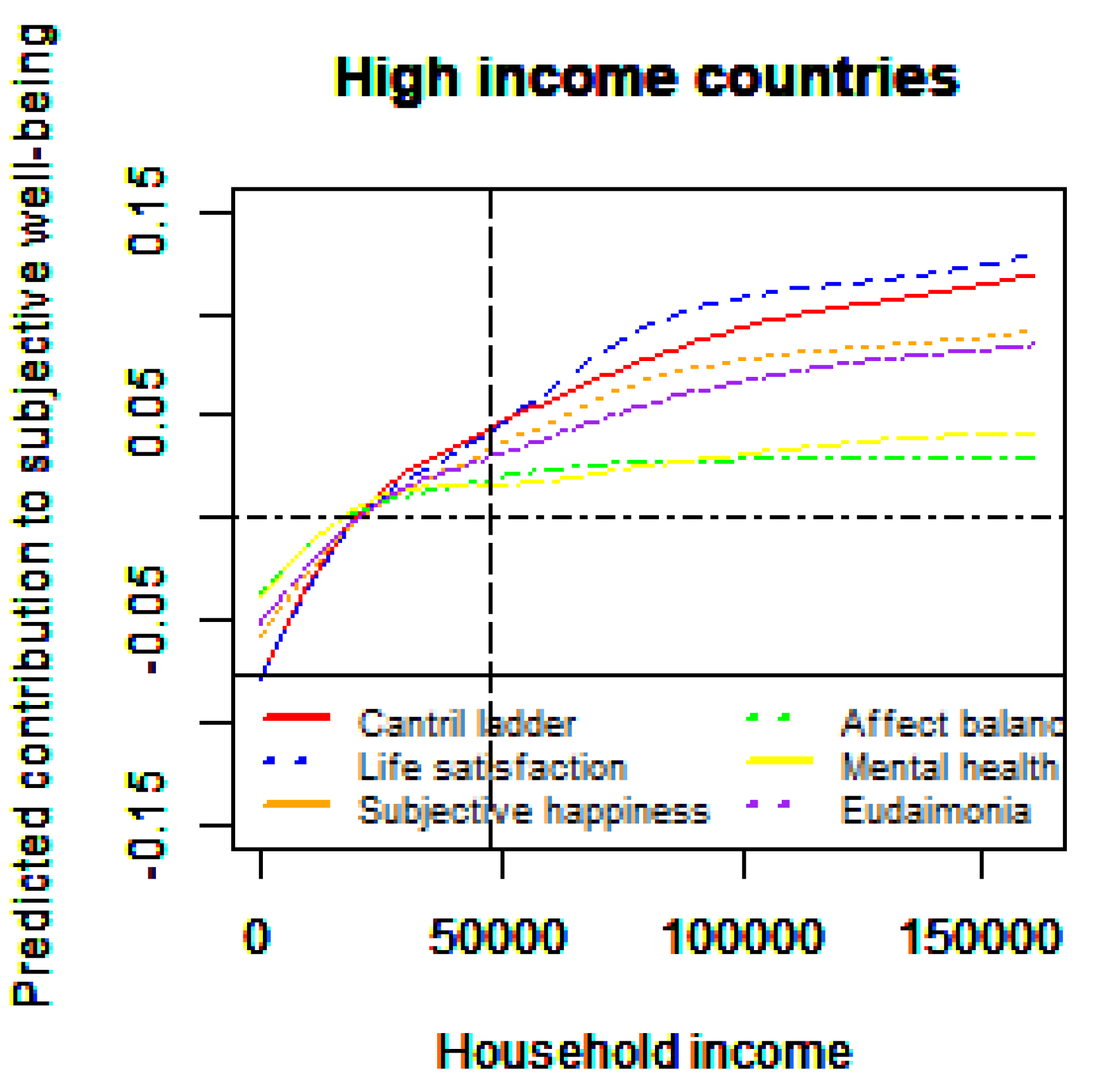
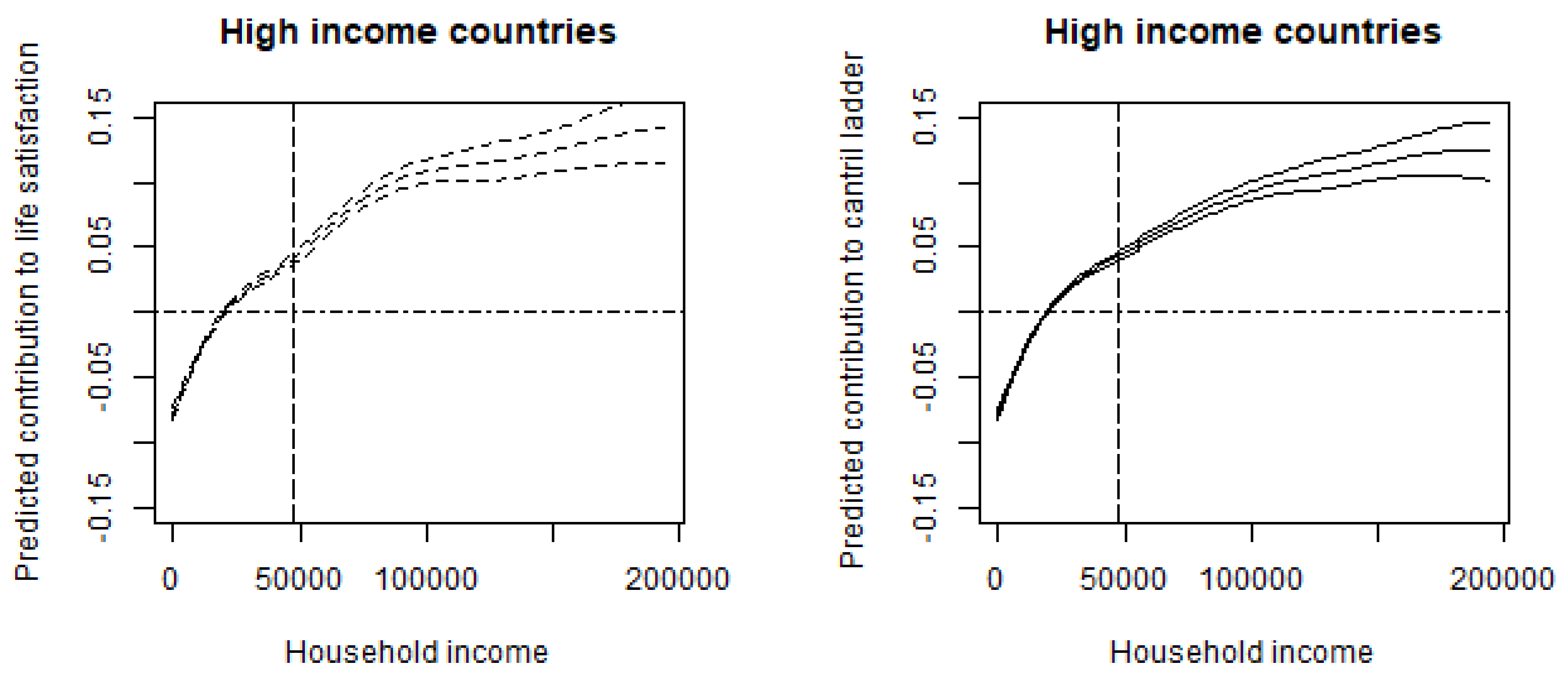
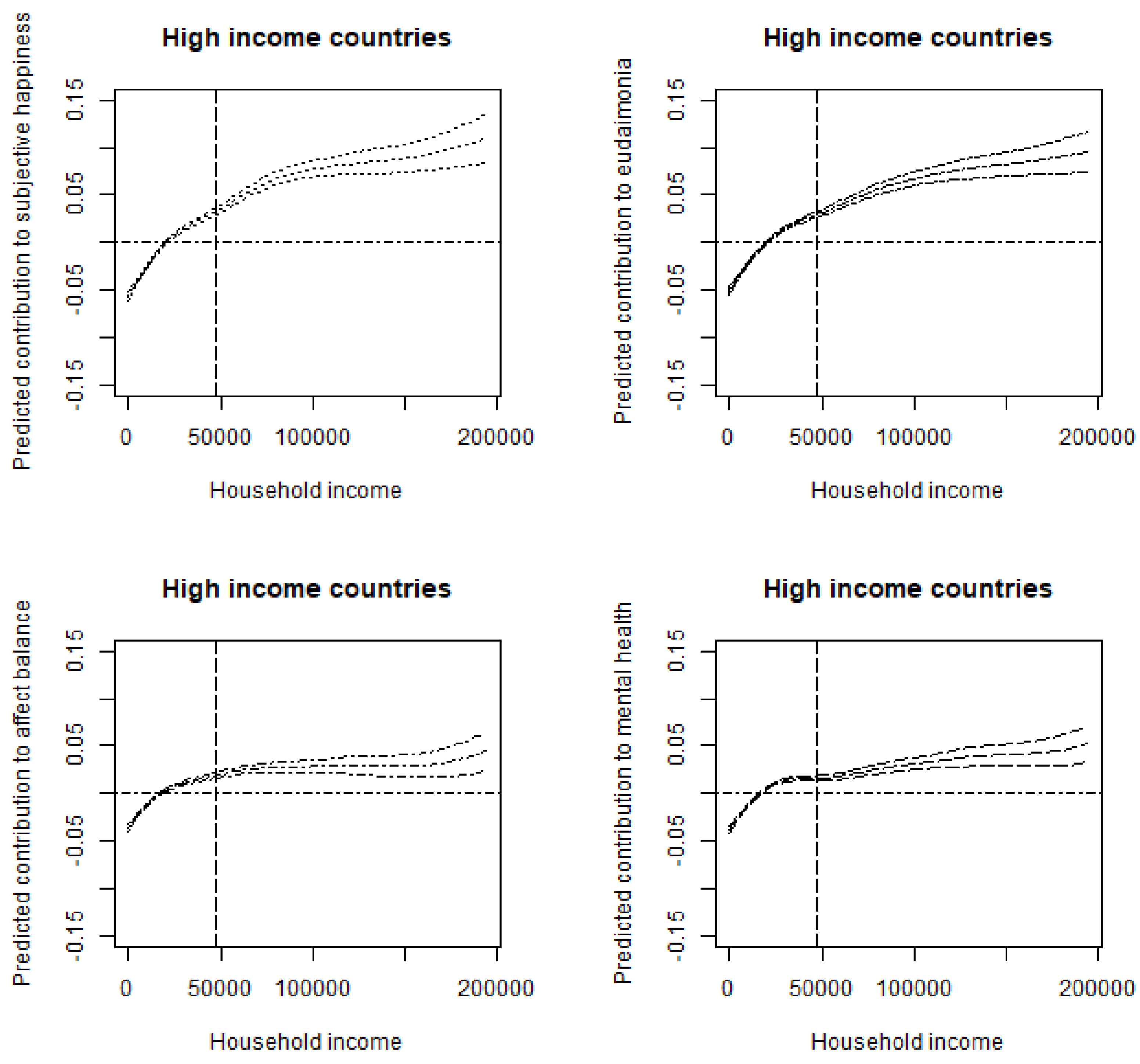
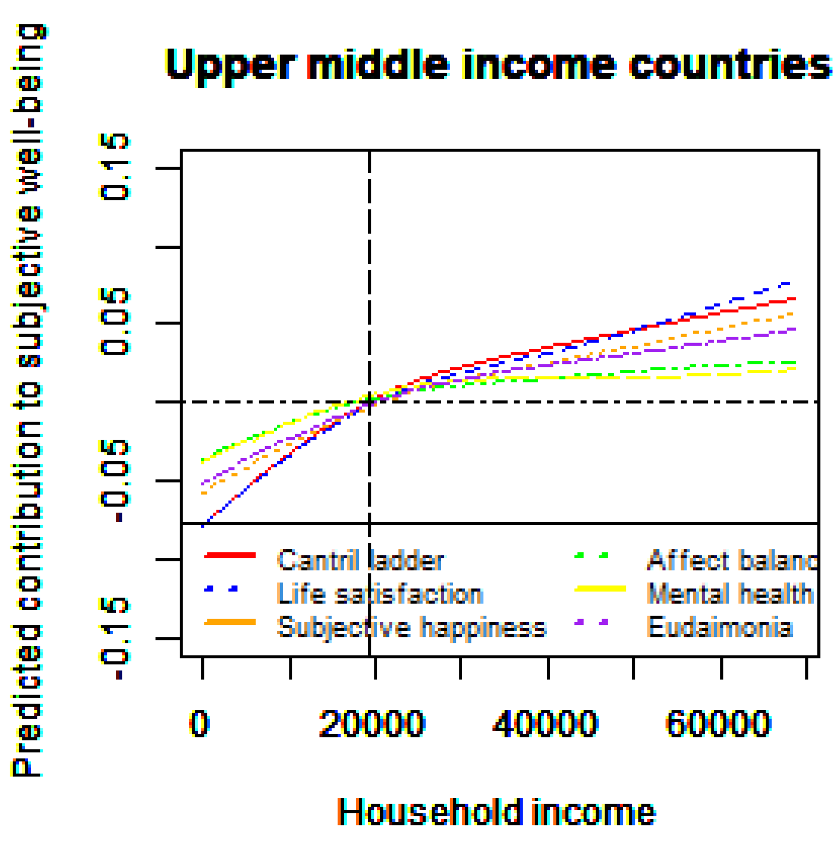
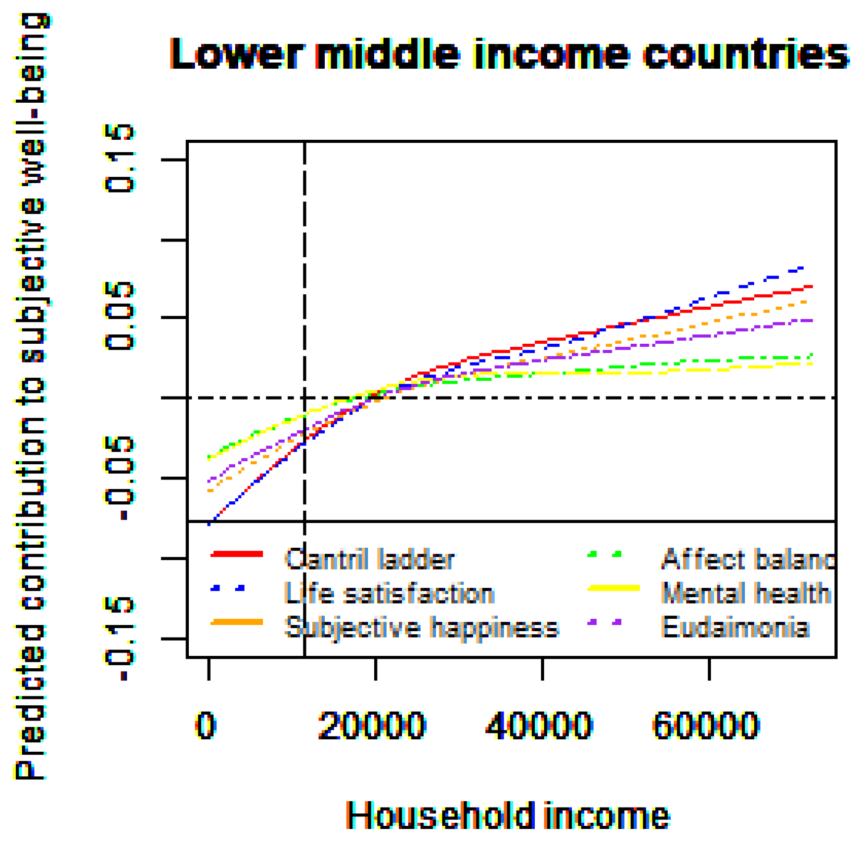
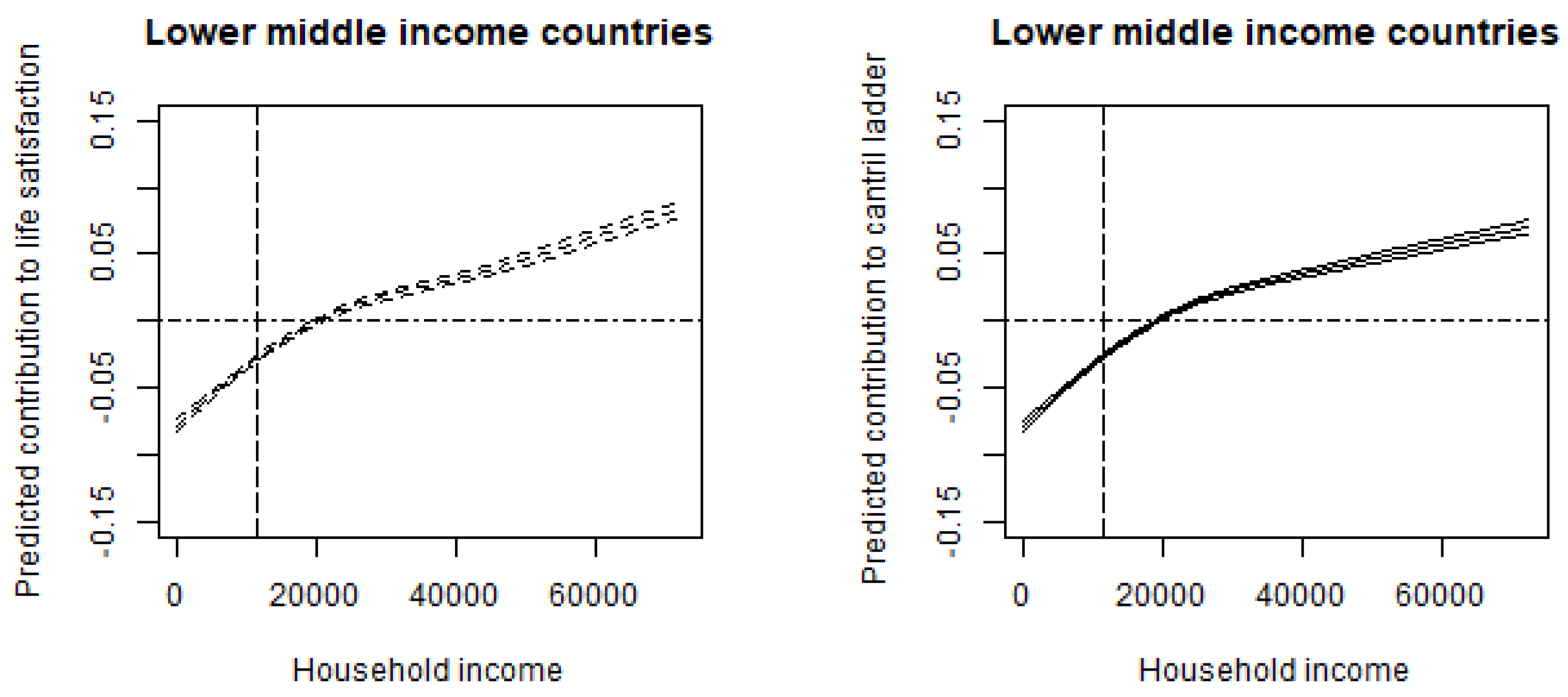
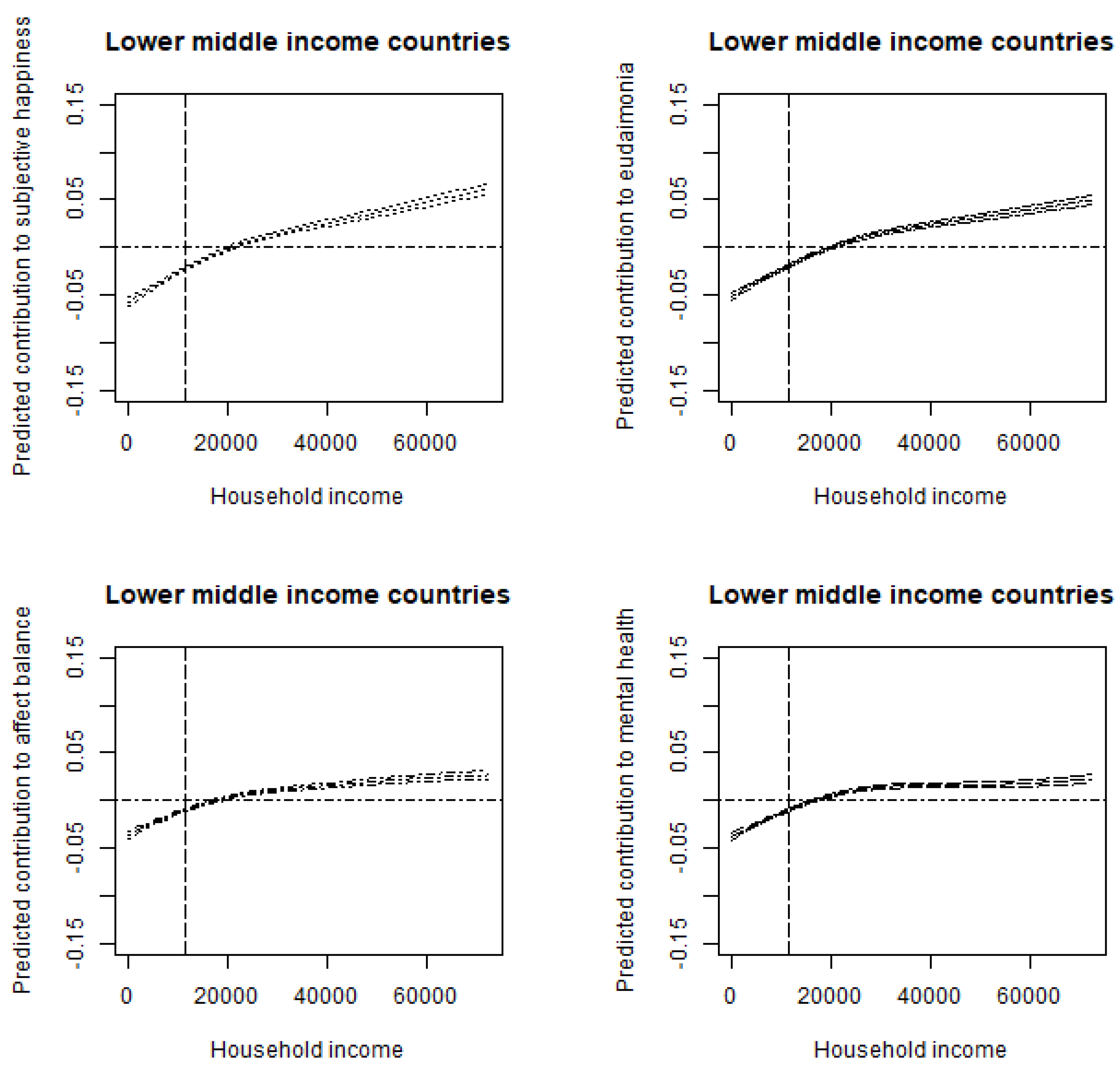
We present the estimation results for high-income (HI) economies in Figure 5 and Figure 6, those for upper middle-income (UM) economies in Figure 7 and Figure 8, and those for lower middle-income (LM) economies in Figure 9 and Figure 10. These results reflect patterns in the slopes that closely resemble those of the aggregated sample shown in Figure 1 and Figure 2; the six SWB indices can be categorized into three groups: (1) affect balance and mental health, (2) subjective happiness and eudaimonia, and (3) life satisfaction and the Cantril Ladder. The estimation results for control variables are shown in

Table 8. Estimated results (high-income countries).

	Model A	Model B	Model C	Model D	Model E	Model F
	Life satisfaction	Cantril ladder	Subjective happiness	Eudaimonia	Affect balance	Mental health
Female dummy	1.33 × 10−2 *** (8.55)	2.27 × 10−2 *** (14.35)	1.98 × 10−2 *** (13.33)	1.54 × 10−2 *** (13.46)	3.63 × 10−2 * (2.34)	−8.85 × 10−2 *** (−7.35)
Age	−5.54 × 10−3 *** (−24.65)	−5.65 × 10−3 *** (−23.39)	−9.43 × 10−3 *** (−23.98)	−5.44 × 10−3 *** (−16.89)	−4.24 × 10−3 *** (−14.46)	−3.53 × 10−3 *** (−13.56)
Age squared	1.22 × 10−4 *** (24.43)	5.43 × 10−5 *** (24.34)	1.04 × 10−4 *** (24.47)	6.33 × 10−5 *** (24.34)	5.54 × 10−5 *** (16.47)	5.25 × 10−5 *** (13.23)
Marital dummy	5.54 × 10−2 *** (32.97)	4.67 × 10−2 *** (28.23)	6.54 × 10−2 *** (37.44)	4.23 × 10−2 *** (25.27)	2.86 × 10−2 *** (19.45)	2.24 × 10−2 *** (18.34)
Constant term	5.64 × 10−1 *** (95.75)	5.26 × 10−1 *** (105.77)	7.74 × 10−1 *** (113.42)	6.65 × 10−1 *** (109.38)	6.06 × 10−1 *** (105.54)	6.42 × 10−1 *** (124.73)
Approximate significance of smooth terms (F values)	240.7 ***	264.7 ***	228.0 ***	237.7 ***	126.7 ***	157.9 ***
Generalized cross validation (GCV)	23.74	26.64	25.28	27.32	27.35	26.74
Adjusted R squared	0.124	0.123	0.105	0.154	0.096	0.106
Time-fixed effects	Yes	Yes	Yes	Yes	Yes	Yes
Country-fixed effects	Yes	Yes	Yes	Yes	Yes	Yes
Observations	40,520	40,520	40,520	40,520	40,520	40,520

Note: Values in parentheses are t-values. * and *** indicate “significant” at the 10% level and the 1% level, respectively.

,

Table 9. Estimated results (upper middle-income countries).

	Model A	Model B	Model C	Model D	Model E	Model F
	Life satisfaction	Cantril ladder	Subjective happiness	Eudaimonia	Affect balance	Mental health
Female dummy	1.25 × 10−2 *** (9.23)	2.43 × 10−2 *** (15.13)	1.86 × 10−2 *** (11.21)	1.42 × 10−2 *** (11.85)	2.53 × 10−2 *** (2.65)	−7.53 × 10−2 *** (−3.24)
Age	−4.78 × 10−3 *** (−23.43)	−4.59 × 10−3 *** (−20.04)	−7.21 × 10−3 *** (−21.54)	−5.25 × 10−3 *** (−13.64)	−4.31 × 10−3 *** (−12.63)	−4.53 × 10−3 *** (−11.12)
Age squared	1.32 × 10−4 *** (23.96)	5.21 × 10−5 *** (16.53)	1.22 × 10−4 *** (26.25)	5.52 × 10−5 *** (20.76)	5.75 × 10−5 *** (13.66)	5.35 × 10−5 *** (14.76)
Marital dummy	5.11 × 10−2 *** (23.53)	4.26 × 10−2 *** (22.79)	6.33 × 10−2 *** (23.43)	4.55 × 10−2 *** (15.34)	2.31 × 10−2 *** (16.80)	2.12 × 10−2 *** (15.74)
Constant term	5.42 × 10−1 *** (87.85)	3.36 × 10−1 *** (103.46)	4.44 × 10−1 *** (132.367)	6.53 × 10−1 *** (103.75)	6.25 × 10−1 *** (113.78)	6.42 × 10−1 *** (113.44)
Approximate significance of smooth terms (F values)	223.7 ***	253.3 ***	225.1 ***	242.5 ***	141.4 ***	134.9 ***
Generalized cross validation (GCV)	21.53	23.34	22.14	26.69	25.57	23.35
Adjusted R squared	0.125	0.122	0.101	0.143	0.091	0.112
Time-fixed effects	Yes	Yes	Yes	Yes	Yes	Yes
Country-fixed effects	Yes	Yes	Yes	Yes	Yes	Yes
Observations	31,849	31,849	31,849	31,849	31,849	31,849

Note: Values in parentheses are t-values. *** indicates “significant” at the 1% level.

and

Table 10. Estimated results (lower middle-income countries).

	Model A	Model B	Model C	Model D	Model E	Model F
	Life satisfaction	Cantril ladder	Subjective happiness	Eudaimonia	Affect balance	Mental health
Female dummy	1.51 × 10−2 *** (3.21)	2.14 × 10−2 *** (6.26)	1.86 × 10−2 *** (4.35)	1.32 × 10−2 *** (7.41)	3.21 × 10−2 * (2.34)	−5.64 × 10−2 *** (−3.64)
Age	−5.31 × 10−3 *** (−8.42)	−5.23 × 10−3 *** (−13.67)	−9.34 × 10−3 *** (−13.86)	−5.21 × 10−3 *** (−9.32)	−3.42 × 10−3 *** (−7.79)	−3.23 × 10−3 *** (−5.46)
Age squared	1.41 × 10−4 *** (13.31)	5.49 × 10−5 *** (15.32)	1.24 × 10−4 *** (12.52)	2.36 × 10−5 *** (13.78)	4.76 × 10−5 *** (7.23)	5.35 × 10−5 *** (4.35)
Marital dummy	5.45 × 10−2 *** (23.97)	4.32 × 10−2 *** (15.68)	4.53 × 10−2 *** (24.68)	4.35 × 10−2 *** (12.36)	1.46 × 10−2 *** (11.97)	2.36 × 10−2 *** (10.36)
Constant term	2.35 × 10−1 *** (56.97)	3.96 × 10−1 *** (64.34)	2.97 × 10−1 *** (45.08)	3.99 × 10−1 *** (56.36)	4.26 × 10−1 *** (41.57)	3.56 × 10−1 *** (47.35)
Approximate significance of smooth terms (F values)	143.6 ***	153.4 ***	143.3 ***	142.4 ***	93.2 ***	104.3 ***
Generalized cross validation (GCV)	13.35	18.34	21.35	23.24	24.324	25.32
Adjusted R squared	0.113	0.114	0.093	0.134	0.086	0.078
Time-fixed effects	Yes	Yes	Yes	Yes	Yes	Yes
Country-fixed effects	Yes	Yes	Yes	Yes	Yes	Yes
Observations	13,805	13,805	13,805	13,805	13,805	13,805

Note: Values in parentheses are t-values. * and *** indicate “significant” at the 10% level and the 1% level, respectively.

.

6. Discussion and Conclusions

We investigated the relationship between income and SWB using six distinct SWB measures. Based on our findings, we categorized these measures into two groups: Group (a), comprising life satisfaction, the Cantril Ladder, subjective happiness, and eudaimonia; and Group (b), consisting of mental health and affect balance.

Our results indicate that the slopes for Group (b) are significantly smaller than those for Group (a). This observation aligns with Kahneman and Deaton [1], who found that while income boosts life evaluations in the United States, it has a limited impact on emotional well-being beyond a certain threshold. The findings also concur with Phillips [67], who distinguished between hedonic and eudaimonic happiness, and with Vitterso et al. [24], who discussed the theoretical divide between hedonic and eudaimonic well-being. Moreover, our results support existing studies that differentiate cognitive from affective components of SWB.

Despite these differences, both groups exhibit a common pattern. For all SWB indexes, the slope is positive but diminishes as it approaches approximately USD 20,000, with a pronounced decline around this level. This suggests that USD 20,000 may be a pivotal income threshold at which individuals can adequately address their basic needs. Notably, this benchmark appears relevant for both developing and developed countries, indicating a potentially universal trend.

Furthermore, our estimation results allow us to classify the six SWB measures into three groups: (1) mental health and affect balance, (2) subjective happiness and eudaimonia, and (3) life satisfaction and the Cantril Ladder. While the income–SWB relationships for the Cantril Ladder and life satisfaction are nearly identical, subjective happiness generally shows a shallower upward trend—consistent with Diener et al. [24]—suggesting that subjective happiness is more susceptible to emotional factors. Eudaimonia also tends to rise more slowly than the Cantril Ladder, and the income–SWB relationships for subjective happiness and eudaimonia follow a similar pattern. This finding is in line with Sanjuan [25], who distinguished eudaimonia, subjective happiness, and life satisfaction, arguing that eudaimonic well-being may influence prudential happiness or life satisfaction via hedonic well-being. It also aligns with the findings of Peterson et al. [22], who developed a measure grounded in Seligman’s theory of authentic happiness, encompassing hedonic well-being (group (1)), eudaimonia (group (2)), and life satisfaction (group (3)). Similarly, it resonates with Haybron [68], who categorized happiness into three philosophical components: psychological (pleasant life, group (1)), perfectionist (meaningful life, group (2)), and prudential (engaged life, group (3)).

We need to note that income is closely tied to consumption, which refers to the goods and services people actually use to satisfy needs and desires. Many economists argue that consumption is the more direct indicator of material well-being, since individuals derive utility from consuming rather than from income per se [44]. Empirical studies using household consumption expenditure in place of income often find similar patterns for SWB. For example, analyses of panel survey data in developed countries show that life satisfaction increases with higher consumption expenditure [44]. People with more spending power, evidenced by greater consumption, tend to report greater satisfaction with their lives, confirming that material conditions influence well-being whether measured by earnings or spending. In poor countries or communities, consumption (especially of basic necessities) is a critical driver of happiness: the ability to eat, have shelter, and access essentials translates directly into life satisfaction and positive affect. A study in Germany found that spending on certain categories—especially leisure and recreation—had positive effects on happiness, whereas spending on basic goods like food and housing (which everyone must buy to a certain extent) showed no significant impact once other factors were controlled [44].

Numerous studies suggest that unprecedented reductions in consumption are needed to stay within planetary boundaries [69,70]. Evidence indicates that humanity is already overshooting critical Earth-system thresholds, largely due to high consumption in developed nations [69,70,71]. Recent analyses warn that achieving a “safe and just” operating space may require cutting resource throughput by at least 50–70% globally [72]. These findings imply that developed nations must scale down resource use and that developing nations should avoid replicating developed nations’ resource-intensive growth trajectories [73].

Meanwhile, well-being research shows that SWB does not increase indefinitely with rising income ([74,75]), a phenomenon known as the “Easterlin paradox.” Beyond a certain threshold, additional income yields diminishing returns to SWB [1,76]. Therefore, unless societies can enhance the SWB gained per unit of consumption—or per unit of income—efforts to reduce consumption in line with ecological limits may come at the cost of lower well-being [77]. A key challenge for policymakers is to foster non-material, low-resource drivers of SWB, allowing both developed and developing nations to prosper within planetary boundaries [72,73].

As Tsurumi et al. [77] discuss, global consumption patterns are currently unsustainable. Developed countries must lower per capita consumption to remain within Earth’s environmental limits, and developing countries experiencing economic growth must also pursue development while restricting per capita consumption. In this context, enhancing SWB per unit of consumption is crucial. The key question becomes how to improve SWB with minimal consumption—an increasingly pertinent issue for sustainability.

A pivotal consideration in this discourse is the multiplicity of SWB indicators. When investigating the connection between consumption and SWB, the choice of SWB indicator is essential. Because each major SWB index has distinct characteristics, research on the link between economic development and SWB may yield different conclusions depending on the measure employed. Consequently, comparing major SWB indicators—which is the aim of this study—is crucial both for understanding this relationship and for guiding sustainable development policies.

While economic development is often assumed to enhance SWB, our analysis reveals that this relationship does not hold consistently across all SWB indicators. In particular, certain indicators show little or no improvement in well-being despite increasing income levels, suggesting the presence of excessive or inefficient consumption that fails to contribute to genuine human flourishing. These findings challenge the conventional growth-centric paradigm and call for a deeper societal and academic inquiry into what constitutes “true prosperity.” From a sustainability perspective, aligning economic progress with authentic improvements in well-being is essential. This requires not only more careful selection and interpretation of SWB metrics, but also a broader re-evaluation of consumption patterns and policy goals to ensure that future development contributes meaningfully to human and ecological well-being.

Policies that emphasize SWB indicators that tend to increase more readily with income growth may risk accelerating current consumption patterns, which could prove unsustainable. By focusing on SWB indicators that are less responsive to income increases, it may become evident that current consumption levels are not effective in enhancing well-being. This awareness could, in turn, lead to a reconsideration of both the quantity and composition of consumption.

Our study comes with certain limitations. We aimed to procure representative samples for each country, aligning our sampling criteria with the gender and age distribution specific to each nation. As outlined in

Table A2. Data limitation (income).

	Country *	GNI per Capita, Calculated Using the World Bank Atlas Method (Current USD) in 2015	Gallup Self-Reported Median Household Income [USD] in 2013	Our Survey Data: ANNUAL Household Income (USD) (Average)	Our Survey Data: ANNUAL Household Income (USD) (Median)
High-Income Economies (GNI per capita ≥ USD 12,476)	Australia	60,050	46,555	56,011	47,769
	Sweden	57,900	50,514	51,956	43,295
	Canada	57,250	41,280	48,783	41,164
	United States	55,980	43,585	60,126	45,000
	Netherlands	48,850	38,584	44,496	39,093
	Germany	45,790	33,333	45,488	39,093
	United Kingdom	43,700	31,617	53,748	40,191
	France	40,710	31,112	41,092	39,093
	Japan	38,840	33,822	50,899	49,585
	Italy	32,830	20,085	40,641	27,924
	Spain	28,380	21,959	37,593	27,924
	Greece	20,270	17,777	19,587	16,754
	Czech Republic	18,150	22,913	15,166	12,716
	Poland	13,310	15,338	16,821	7963
Upper Middle-Income Economies (GNI per capita = USD 4036–USD 12,475)	Chile	14,100 **	8098	16,013	11,462
	Venezuela	11,780 ***	11,239	34,088	23,841
	Russia	11,450	11,724	11,531	9782
	Malaysia	10,570	11,207	18,708	16,894
	Brazil	9990	7522	15,103	9006
	Mexico	9710	11,680	12,281	9445
	Romania	9510	7322	15,799	6244
	China	7900	6180	20,357	17,481
	Colombia	7140	6544	10,833	8739
	Thailand	5720	7029	17,744	12,263
Lower Middle-Income Economies (GNI per capita = USD 1026–USD 4035)	South Africa	6080 ****	5217	21,803	16,448
	Mongolia	3870	5922	5403	4758
	Sri Lanka	3800	3242	4121	3749
	Philippines	3550	2401	11,318	9228
	Egypt	3340	3111	5768	3584
	Vietnam	1990	4783	7995	6022
	India	1590	3168	14,158	4677
	Myanmar	1160	No data	6602	4645

Note: * Descending order by GNI per capita, calculated using the World Bank Atlas method (current USD) 2015. ** Because the Gallup self-reported median household income in Chile is relatively low compared with HI, we classify Chile as an upper middle-income economy. *** Value in 2013. **** The Gallup self-reported median household income of South Africa is lower than that of upper middle-income economies. Hence, we classify South Africa as a lower middle-income economy.

in the Appendix A, the median household income of our samples aligns closely with the Gallup self-reported median household income for most countries. Nevertheless, deviations do emerge, especially within developing nations. The average or median annual household income from our survey data for some of these countries tends to exceed both the GNI per capita and Gallup’s self-reported median household income. It is worth noting that both online and face-to-face surveys in developing nations often capture respondents from comparatively higher income brackets. As a result, the findings from our estimations should be approached judiciously, especially when considering data from developing countries.

Furthermore,

Table A3. Descriptive statistics for Cantril Ladder by country (mean).

Country *	Cantril Ladder	Cantril Ladder (Gallup Worldwide Research Data)
Australia	6.80	7.27
Sweden	6.88	7.31
Canada	6.86	7.33
United States	6.95	6.89
Netherlands	7.02	7.44
Germany	6.65	6.97
United Kingdom	6.56	6.84
France	6.63	6.49
Japan	5.93	5.92
Italy	6.26	6.00
Spain	6.67	6.31
Greece	6.21	5.36
Czech Republic	6.55	6.71
Poland	6.37	6.12
Chile	7.01	6.48
Venezuela	6.94	4.81
Russia	5.97	5.81
Malaysia	6.48	6.32
Brazil	6.66	6.42
Mexico	7.67	6.49
Romania	7.00	5.95
China	6.76	5.25
Colombia	7.39	6.26
Thailand	6.63	6.07
South Africa	6.38	4.72
Mongolia	6.16	5.13
Sri Lanka	7.03	4.47
Philippines	7.21	5.52
Egypt	6.15	4.42
Vietnam	6.89	5.10
India	7.23	4.19
Myanmar	5.89	4.31

* Descending order by GNI per capita, calculated using the World Bank Atlas method (current USD) 2015.

in the Appendix A shows a comparison between the country averages of the Cantril Ladder in our survey and those from Gallup. We chose the Cantril Ladder for comparison because the questionnaires were the same. Although a large part of the scores is similar between these two datasets for developing countries, the score of our survey data tends to be higher than that of the Gallup data. Here again, it could be related to the existence of relatively higher-income panels in our data compared to the population, which suggests that we need to interpret our estimation results with caution, especially in developing countries.

Additionally, our study converts household income into USD using 2015 exchange rates. This methodological choice may limit the cross-national comparability of the income variable, where USD 1 in nominal terms can have vastly different purchasing power. Future research should consider PPP-adjusted income or consumption-based measures to more accurately reflect material living standards.

A growing body of cross-national research has examined the relationship between income and SWB, using large-scale international datasets such as the World Values Survey (WVS), European Social Survey (ESS), and the Gallup World Poll. These studies generally find a positive correlation between income and SWB across countries, yet the strength and nature of the relationship vary depending on contextual factors such as economic development, cultural norms, and income inequality [32,33]. We aimed to control these contextual factors by including country-fixed effects. However, while the inclusion of country-fixed effects in cross-national analyses helps control for time-invariant national characteristics, it may not fully account for the complex and dynamic influence of cultural context on SWB. Fixed effects models effectively absorb unobserved heterogeneity at the national level, but they do so by treating cultural factors as constant over time and across individuals within a country. In reality, however, cultural norms, value systems, and emotional expression can vary both across subpopulations and over time, influencing not only average levels of SWB but also the meaning and salience of constructs such as income and happiness [78,79].

Moreover, fixed effects do not capture within-country cultural heterogeneity, such as differences in regional identities, ethnic groups, or generational value shifts. Consequently, while fixed effects are valuable for reducing bias due to unobserved country-level characteristics, they are insufficient for fully isolating the cultural mechanisms through which income influences subjective well-being. Researchers seeking to understand these mechanisms must therefore incorporate complementary strategies, such as multi-level modeling, cultural indices (e.g., Hofstede dimensions), or interaction terms that explicitly account for cultural variation.

Although this topic extends beyond the scope of our current study, future research could investigate the specific elements represented by the income variable. As highlighted in our robustness checks, economic development can have both positive and negative effects on SWB. Notably, the predicted contributions for the six SWB indices in models incorporating additional control variables (Figure 3 and Figure 4) are lower than those in the primary models (Figure 1 and Figure 2), suggesting potential spurious correlations involving income.

In addition, variations in consumption patterns across age groups may influence the relationship between income and SWB indicators. Nevertheless, the primary objective of this study is to investigate the average relationship between income and SWB indicators at the population level, with the aim of assessing whether this relationship differs according to the specific indicator employed. Consequently, age-disaggregated analyses fall beyond the scope of the present study and are suggested as a topic for future research.

Furthermore, the surveys conducted prior to the COVID-19 pandemic offer a baseline assessment of SWB under normal conditions. As such, they provide a valuable benchmark against which SWB levels during and after the pandemic can be compared, contingent upon the availability of corresponding data.

References

1. Kahneman, D.; Deaton, A. High income improves evaluation of life but not emotional well-being. Proc. Natl. Acad. Sci. USA 2010, 107, 16489–16493. [Google Scholar] [CrossRef] [PubMed]
2. Killingsworth, M.A. Experienced well-being rises with income, even above $75,000 per year. Proc. Natl. Acad. Sci. USA 2021, 118, e2016976118. [Google Scholar] [CrossRef] [PubMed]
3. Killingsworth, M.A.; Kahneman, D.; Mellers, B. Income and emotional well-being: A conflict resolved. Proc. Natl. Acad. Sci. USA 2023, 120, e2208661120. [Google Scholar] [CrossRef] [PubMed]
4. OECD. Guidelines On Measuring Subjective Well-Being; OECD Publishing: Paris, France, 2013. [Google Scholar] [CrossRef]
5. Jebb, A.T.; Tay, L.; Diener, E.; Oishi, S. Happiness, income satiation and turning points around the world. Nat. Hum. Behav. 2018, 2, 33–38. [Google Scholar] [CrossRef]
6. Diener, E.; Kahneman, D.; Tov, W.; Arora, R. Income’s Association with Judgments of Life Versus Feelings. In International Differences in Well-Being; Diener, E., Helliwell, J., Kahneman, D., Eds.; Oxford University Press: Oxford, UK, 2010; pp. 3–15. [Google Scholar]
7. Stevenson, B.; Wolfers, J. Subjective well-being and income: Is there any evidence of satiation? Am. Econ. Rev. 2013, 103, 598–604. [Google Scholar] [CrossRef]
8. Deaton, A. Income, health, and well-being around the world: Evidence from the Gallup World Poll. J. Econ. Perspect. 2008, 22, 53–72. [Google Scholar] [CrossRef]
9. Reyes-García, V.; Zorondo-Rodríguez, F.; Angelsen, A.; Babigumira, R.; Pyhälä, A.; Wunder, S. Subjective well-being and income: Empirical patterns in the rural developing world. J. Happiness Stud. 2016, 17, 773–791. [Google Scholar] [CrossRef]
10. Adler, A.; Seligman, M. Using wellbeing for public policy: Theory, measurement, and recommendations. Int. J. Wellbeing 2016, 6, 1–35. [Google Scholar] [CrossRef]
11. Helliwell, J.F.; Layard, R.; Sachs, J.D.; De Neve, J.-E.; Aknin, L.B.; Wang, S. (Eds.) World Happiness Report 2022; Sustainable Development Solutions Network: New York, NY, USA, 2022. [Google Scholar]
12. Andrews, F.M.; Withey, S.B. Social Indicators of Well-Being: America’s Perception of Life Quality; Plenum Press: New York, NY, USA, 1976. [Google Scholar]
13. Michalos, A.C. Satisfaction and happiness. Soc. Indic. Res. 1980, 8, 385–422. [Google Scholar] [CrossRef]
14. Veenhoven, R. Is happiness relative? Soc. Indic. Res. 1991, 24, 1–39. [Google Scholar] [CrossRef]
15. Cantril, H. The Pattern of Human Concerns; Rutgers University Press: New Brunswick, NJ, USA, 1965. [Google Scholar]
16. Diener, E. Subjective well-being. Psychol. Bull. 1984, 75, 542–575. [Google Scholar] [CrossRef]
17. Michalos, A.C. Multiple discrepancies theory (MDT). Soc. Indic. Res. 1985, 36, 31–44. [Google Scholar] [CrossRef]
18. Diener, E.; Emmons, R.A.; Larsen, R.J.; Griffin, S. The satisfaction with life scale. J. Pers. Assess. 1985, 49, 71–75. [Google Scholar] [CrossRef]
19. Kozma, A.; Stones, M.J. Longitudinal findings on a componential model of happiness. In Developments in Quality-of-Life Studies in Marketing; Sirgy, M.J., Meadow, H.L., Rahtz, D., Samli, A.C., Eds.; Academy of Marketing Science: Mississippi, MS, USA, 1992; Volume 4, pp. 139–142. [Google Scholar]
20. Parducci, A. Happiness, Pleasure, and Judgment: The Contextual Theory and Its Applications; Lawrence Erlbaum Associates: Mahwah, NJ, USA, 1995. [Google Scholar]
21. Kahneman, D. Objective happiness. In Well-Being: The Foundations of Hedonic Psychology; Kahneman, D., Diener, E., Schwartz, N., Eds.; Russell Sage: New York, NY, USA, 1999; pp. 3–25. [Google Scholar]
22. Peterson, C.; Park, N.; Seligman, M.E.P. Orientations to happiness and life satisfaction: The full life versus the empty life. J. Happiness Stud. 2005, 6, 25–41. [Google Scholar] [CrossRef]
23. Seligman, M.E.P. Authentic Happiness: Using the New Positive Psychology to Realize Your Potential for Lasting Fulfillment; Free Press: New York, NY, USA, 2002. [Google Scholar]
24. Vittersø, J.; Soholt, Y.; Hetland, A.; Thoresen, I.A.; Røysamb, E. Was Hercules happy? Some answers from a functional model of human well-being. Soc. Indic. Res. 2010, 95, 1–18. [Google Scholar] [CrossRef]
25. Sanjuan, P. Affect balance as a mediating variable between effective psychological functioning and satisfaction with life. J. Happiness Stud. 2011, 12, 373–384. [Google Scholar] [CrossRef]
26. Powdthavee, N.; Van den Berg, B. Putting different price tags on the same health condition: Re-evaluating the well-being valuation approach. J. Health Econ. 2011, 30, 1032–1043. [Google Scholar] [CrossRef]
27. Guthrie, E.; Black, D.; Bagalkote, H.; Shaw, C.; Campbell, M.; Creed, F. Psychological stress and burnout in medical students: A five–year prospective longitudinal study. J. R. Soc. Med. 1998, 91, 237–243. [Google Scholar] [CrossRef]
28. Welsch, H.; Kühling, J. Determinants of pro-environmental consumption: The role of reference groups and routine behavior. Ecol. Econ. 2009, 69, 166–176. [Google Scholar] [CrossRef]
29. Hastie, T.J.; Tibshirani, R.J. Generalized Additive Models; Chapman and Hall: Boca Raton, FL, USA, 1990. [Google Scholar]
30. Blanchflower, D.G.; Oswald, A.J. Is well-being U-shaped over the life cycle? Soc. Sci. Med. 2008, 66, 1733–1749. [Google Scholar] [CrossRef]
31. Frijters, P.; Beatton, T. The mystery of the U-shaped relationship between happiness and age. J. Econ. Behav. Organ. 2012, 82, 525–542. [Google Scholar] [CrossRef]
32. Diener, E.; Tay, L.; Oishi, S. Rising income and the subjective well-being of nations. J. Personal. Soc. Psychol. 2013, 104, 267–276. [Google Scholar] [CrossRef] [PubMed]
33. Helliwell, J.F.; Huang, H.; Wang, S. The social foundations of world happiness. In World Happiness Report 2017; Helliwell, J.F., Layard, R., Sachs, J., Eds.; Sustainable Development Solutions Network: New York, NY, USA, 2017; pp. 8–47. [Google Scholar]
34. Wood, S.N. Stable and efficient multiple smoothing parameter estimation for generalized additive models. J. Am. Stat. Assoc. 2004, 99, 673–686. [Google Scholar] [CrossRef]
35. Wood, S.N. Fast stable direct fitting and smoothness selection for generalized additive models. J. R. Stat. Soc. Ser. B Stat. Methodol. 2008, 70, 495–518. [Google Scholar] [CrossRef]
36. Wood, S.N. Generalized Additive Models: An Introduction with R, 2nd ed.; CRC Press: Boca Raton, FL, USA, 2017. [Google Scholar]
37. Diener, E.; Inglehart, R.; Tay, L. Theory and validity of life satisfaction scales. Soc. Indic. Res. 2013, 112, 497–527. [Google Scholar] [CrossRef]
38. Cheung, F.; Lucas, R.E. Assessing the validity of single-item life satisfaction measures: Results from three large samples. Qual. Life Res. 2014, 23, 2809–2818. [Google Scholar] [CrossRef]
39. Pavot, W.; Diener, E. Review of the Satisfaction With Life Scale. Psychol. Assess. 1993, 5, 164–172. [Google Scholar] [CrossRef]
40. Schimmack, U. Affect measurement in experience sampling research. J. Happiness Stud. 2003, 4, 79–106. [Google Scholar] [CrossRef]
41. Watson, D.; Tellegen, A. Issues in the dimensional structure of affect—Effects of descriptors, measurement scales, and rotation of factors. J. Personal. Soc. Psychol. 1999, 76, 820–838. [Google Scholar] [CrossRef]
42. Goldberg, D.; Gater, R.; Sartorius, N.; Ustun, T.B.; Piccinelli, M.; Gureje, O.; Rutter, C. The validity of two versions of the GHQ in the WHO study of mental illness in general health care. Psychol. Med. 1997, 27, 191–197. [Google Scholar] [CrossRef]
43. Jackson, C. The General Health Questionnaire. Occup. Med. 2007, 57, 79. [Google Scholar] [CrossRef]
44. Di Tella, R.; MacCulloch, R. Gross national happiness as an answer to the Easterlin Paradox? J. Dev. Econ. 2008, 86, 22–42. [Google Scholar] [CrossRef]
45. Tsurumi, T.; Managi, S. Monetary valuations of life conditions in a consistent framework: The life satisfaction approach. J. Happiness Stud. 2017, 18, 1275–1303. [Google Scholar] [CrossRef]
46. Putnam, R.D. Democracies in Flux: The Evolution of Social Capital in Contemporary Society; Oxford University Press: Oxford, UK, 2004. [Google Scholar]
47. Frey, B.S.; Stutzer, A. What can economists learn from happiness research? J. Econ. Lit. 2002, 40, 402–435. [Google Scholar] [CrossRef]
48. Pouwels, B.; Siegers, J.; Vlasblom, J.D. Income, working hours, and happiness. Econ. Lett. 2008, 99, 72–74. [Google Scholar] [CrossRef]
49. Yamashita, T.; Bardo, A.R.; Liu, D. Are East Asians happy to work more or less? Associations between working hours, relative income and happiness in China, Japan, South Korea and Taiwan. Asian J. Soc. Psychol. 2016, 19, 264–274. [Google Scholar] [CrossRef]
50. Welsch, H. Preferences over prosperity and pollution: Environmental valuation based on happiness surveys. Kyklos 2002, 55, 473–494. [Google Scholar] [CrossRef]
51. Welsch, H. Environment and happiness: Valuation of air pollution using life satisfaction data. Ecol. Econ. 2006, 58, 801–813. [Google Scholar] [CrossRef]
52. Welsch, H. Environmental welfare analysis: A life satisfaction approach. Ecol. Econ. 2007, 62, 544–551. [Google Scholar] [CrossRef]
53. Rehdanz, K.; Maddison, D. Local environmental quality and life satisfaction in Germany. Ecol. Econ. 2008, 64, 787–797. [Google Scholar] [CrossRef]
54. Luechinger, S. Life satisfaction and transboundary air pollution. Econ. Lett. 2010, 107, 4–6. [Google Scholar] [CrossRef]
55. Mackerron, G.; Mourato, S. Life satisfaction and air quality in London. Ecol. Econ. 2009, 68, 1441–1453. [Google Scholar] [CrossRef]
56. Ferreira, S.; Moro, M. On the use of subjective well-being data for environmental valuation. Environ. Resour. Econ. 2010, 46, 249–273. [Google Scholar] [CrossRef]
57. Menz, T. Do people habituate to air pollution? Evidence from international life satisfaction data. Ecol. Econ. 2011, 71, 211–219. [Google Scholar] [CrossRef]
58. Ferreira, S.; Akay, A.; Brereton, F.; Cunado, J.; Martinsson, P.; Moro, M.; Ningal, T.F. Life satisfaction and air quality in Europe. Ecol. Econ. 2013, 88, 1–10. [Google Scholar] [CrossRef]
59. Ambrey, C.L.; Fleming, C.M.; Chan, A.Y. Estimating the cost of air pollution in South East Queensland: An application of the life satisfaction non-market valuation approach. Ecol. Econ. 2014, 97, 172–181. [Google Scholar] [CrossRef]
60. Ambrey, C.L.; Fleming, C.M. Valuing scenic amenity using life satisfaction data. Ecol. Econ. 2011, 72, 106–115. [Google Scholar] [CrossRef]
61. Ambrey, C.L.; Fleming, C.M. Public greenspace and life satisfaction in urban Australia. Urban Stud. 2014, 51, 1290–1321. [Google Scholar] [CrossRef]
62. Mackerron, G.; Mourato, S. Happiness is greater in natural environments. Glob. Environ. Change 2013, 23, 992–1000. [Google Scholar] [CrossRef]
63. Tsurumi, T.; Managi, S. Environmental value of green spaces in Japan: An application of the life satisfaction approach. Ecol. Econ. 2015, 120, 1–12. [Google Scholar] [CrossRef]
64. Tsurumi, T.; Imauji, A.; Managi, S. Greenery and well-being: Assessing the monetary value of greenery by type. Ecol. Econ. 2018, 148, 152–169. [Google Scholar] [CrossRef]
65. Cohen, M.A. The effect of crime on life satisfaction. J. Leg. Stud. 2008, 37, S325–S353. [Google Scholar] [CrossRef]
66. Ambrey, C.L.; Fleming, C.M.; Manning, M. Perception or reality: What matters most when it comes to crime in your neighbourhood? Soc. Indic. Res. 2013, 119, 877–896. [Google Scholar] [CrossRef]
67. Phillips, D. Quality of Life: Concept, Policy and Practice; Routledge: London, UK, 2006. [Google Scholar]
68. Haybron, D.M. Two philosophical problems in the study of happiness. J. Happiness Stud. 2000, 1, 207–225. [Google Scholar] [CrossRef]
69. Rockström, J.; Steffen, W.; Noone, K.; Persson, Å.; Chapin, F.S.; Lambin, E.F.; Lenton, T.M.; Scheffer, M.; Folke, C.; Schellnhuber, H.J.; et al. A safe operating space for humanity. Nature 2009, 461, 472–475. [Google Scholar] [CrossRef]
70. Steffen, W.; Richardson, K.; Rockström, J.; Cornell, S.E.; Fetzer, I.; Bennett, E.M.; Biggs, R.; Carpenter, S.R.; De Vries, W.; De Wit, C.A.; et al. Planetary boundaries: Guiding human development on a changing planet. Science 2015, 347, 1259855. [Google Scholar] [CrossRef]
71. Wiedmann, T.; Lenzen, M.; Keyßer, L.T.; Steinberger, J.K. Scientists’ warning on affluence. Nat. Commun. 2020, 11, 3107. [Google Scholar] [CrossRef]
72. O’Neill, D.W.; Fanning, A.L.; Lamb, W.F.; Steinberger, J.K. A good life for all within planetary boundaries. Nat. Sustain. 2018, 1, 88–95. [Google Scholar] [CrossRef]
73. Raworth, K. Doughnut Economics: Seven Ways to Think Like a 21st-Century Economist; Random House Business: London, UK, 2017. [Google Scholar]
74. Easterlin, R.A. Does economic growth improve the human lot? Some empirical evidence. In Nations and Households in Economic Growth; David, P.A., Reder, M.W., Eds.; Academic Press: New York, NY, USA, 1974; pp. 89–125. [Google Scholar]
75. Easterlin, R.A.; McVey, L.A.; Switek, M.; Sawangfa, O.; Zweig, J.S. The happiness–income paradox revisited. Proc. Natl. Acad. Sci. USA 2010, 107, 22463–22468. [Google Scholar] [CrossRef]
76. Clark, A.E.; Flèche, S.; Layard, R.; Powdthavee, N.; Ward, G. The Origins of Happiness: The Science of Well-Being Over the Life Course; Princeton University Press: Princeton, NJ, USA, 2018. [Google Scholar]
77. Tsurumi, T.; Yamaguchi, R.; Kagohashi, K.; Managi, S. Material and relational consumption to improve subjective well-being: Evidence from rural and urban Vietnam. J. Clean. Prod. 2021, 310, 127499. [Google Scholar] [CrossRef]
78. Tov, W.; Diener, E. Culture and subjective well-being. In Handbook of Cultural Psychology; Kitayama, S., Cohen, D., Eds.; Guilford Press: New York, NY, USA, 2007; pp. 691–713. [Google Scholar]
79. Mesquita, B. Emotions as dynamic cultural phenomena. In Handbook of Affective Sciences; Davidson, R.J., Scherer, K.R., Goldsmith, H.H., Eds.; Oxford University Press: Oxford, UK, 2003; pp. 871–890. [Google Scholar]
Figure 1. Relationship between household income and subjective well-being with all data. Notes: The vertical dotted line corresponds to the sample average of household income. To account for outliers, households with incomes exceeding the 99th percentile income level are excluded, restricting the horizontal axis to the range from USD 0 to the 99th percentile of household income in each country. The control variables include gender, age, age squared, marital status, year dummy (time-fixed effects), and country dummies (country-fixed effects).
Sustainability 17 05266 g001
Figure 2. Relationship between household income and subjective well-being with all data by SWB indexes. Notes: The upper and lower lines represent a 95% confidence interval calculated through a Bayesian approach. The vertical dotted line corresponds to the sample average of household income. To account for outliers in each figure, households with incomes above the 99th percentile income level are excluded, resulting in a restricted horizontal axis ranging from USD 0 to the 99th percentile of household income in each country. The control variables include gender, age, age squared, marital status, year dummy (time-fixed effects), and country dummies (country-fixed effects).
Sustainability 17 05266 g002
Figure 3. Relationship between household income and subjective well-being with all data (including additional control variables). Notes: The vertical dotted line corresponds to the sample average of household income. To account for outliers, households with incomes exceeding the 99th percentile income level are excluded, restricting the horizontal axis to the range from USD 0 to the 99th percentile of household income in each country. The control variables include gender, age, age squared, marital status, subjective health, social capital, working hours, environment, safety, year dummy (time-fixed effects), and country dummies (country-fixed effects).
Sustainability 17 05266 g003
Figure 4. Relationship between household income and subjective well-being with all data by SWB indexes (including additional control variables). Notes: The upper and lower lines represent a 95% confidence interval calculated through a Bayesian approach. The vertical dotted line corresponds to the sample average of household income. To account for outliers in each figure, households with incomes above the 99th percentile income level are excluded, resulting in a restricted horizontal axis ranging from USD 0 to the 99th percentile of household income in each country. The control variables include gender, age, age squared, marital status, subjective health, social capital, working hours, safety, year dummy (time-fixed effects), and country dummies (country-fixed effects).
Sustainability 17 05266 g004
Figure 5. Relationship between household income and subjective well-being for subsamples (high-income countries) Notes: The vertical dotted line represents the sample average of household income. The high-income economies include Australia, the United States, Sweden, the Netherlands, the United Kingdom, Canada, Germany, France, Japan, Italy, Spain, Greece, the Czech Republic, and Poland. To account for outliers in each figure, households with incomes above the 99th percentile are excluded, constraining the horizontal axis to the range from USD 0 to the 99th percentile of household income in each country. The control variables include gender, age, age squared, marital status, year dummy (time-fixed effects), and country dummies (country-fixed effects).
Sustainability 17 05266 g005
Figure 6. Relationship between household income and subjective well-being for subsamples by SWB indexes (high-income countries) Notes: The upper and lower lines correspond to a 95% confidence interval using a Bayesian approach. The vertical dotted line corresponds to the sample average of household income. High-income economies are Australia, United States, Sweden, the Netherlands, United Kingdom, Canada, Germany, France, Japan, Italy, Spain, Greece, Czech Republic, and Poland. To consider outliers, for each figure, we eliminate households with income above the 99th percentile income level, limiting the horizontal axis (USD 0 to 99th percentile of household income in each county). Control variables are gender, age, age squared, marital status, year dummy (time-fixed effects), and country dummy (country-fixed effects).
Sustainability 17 05266 g006aSustainability 17 05266 g006b
Figure 7. Relationship between household income and subjective well-being for subsamples (Upper middle-income countries) Notes: The vertical dotted line corresponds to the sample average of household income. Upper middle-income economies are Brazil, China, Colombia, Chile, Malaysia, Mexico, Russia, Romania, Thailand, and Venezuela. To consider outliers, for each figure, we eliminate households with income above the 99th percentile income level, limiting the horizontal axis (USD 0 to 99th percentile of household income in each county). The control variables include gender, age, age squared, marital status, year dummy (time-fixed effects), and country dummies (country-fixed effects).
Sustainability 17 05266 g007
Figure 8. Relationship between household income and subjective well-being for subsamples by SWB indexes (Upper middle-income countries) Notes: The upper and lower lines correspond to a 95% confidence interval using a Bayesian approach. The vertical dotted line corresponds to the sample average of household income. Upper middle-income economies are Brazil, China, Colombia, Chile, Malaysia, Mexico, Russia, Romania, Thailand, and Venezuela. To consider outliers, for each figure, we eliminate households with income above the 99th percentile income level, limiting the horizontal axis (USD 0 to 99th percentile of household income in each county). The control variables include gender, age, age squared, marital status, year dummy (time-fixed effects), and country dummies (country-fixed effects).
Sustainability 17 05266 g008
Figure 9. Relationship between household income and subjective well-being for subsamples (lower middle-income countries) Notes: The vertical dotted line corresponds to the sample average of household income. Lower middle-income economies are Egypt, India, Mongolia, Myanmar, the Philippines, South Africa, Sri Lanka, and Vietnam. To consider outliers, for each figure, we eliminate households with income above the 99th percentile income level, limiting the horizontal axis (USD 0 to 99th percentile of household income in each county). The control variables include gender, age, age squared, marital status, year dummy (time-fixed effects), and country dummies (country-fixed effects).
Sustainability 17 05266 g009
Figure 10. Relationship between household income and subjective well-being for subsamples (lower middle-income countries) Notes: The upper and lower lines correspond to a 95% confidence interval using a Bayesian approach. The vertical dotted line corresponds to the sample average of household income. Lower middle-income economies are Egypt, India, Mongolia, Myanmar, the Philippines, South Africa, Sri Lanka, and Vietnam. To consider outliers, for each figure, we eliminate households with income above the 99th percentile income level, limiting the horizontal axis (USD 0 to 99th percentile of household income in each county). Control variables are gender, age, age squared, marital status, year dummy (time-fixed effects), and country dummy (country-fixed effects).
Sustainability 17 05266 g010aSustainability 17 05266 g010b