Forecast Natural Gas Price by an Extreme Learning Machine Framework Based on Multi-Strategy Grey Wolf Optimizer and Signal Decomposition

Abstract

Natural gas is one of the most important sources of energy in modern society. However, its strong volatility highlights the importance of accurately forecasting natural gas price trends and movements. The nonlinear nature of the natural gas price series makes it difficult to capture. Therefore, we propose a forecasting framework based on signal decomposition and intelligent optimization algorithms to predict natural gas prices. In this forecasting framework, we implement point, probability interval, and quantile interval forecasting. First, the natural gas price sequence is decomposed into multiple Intrinsic Mode Functions (IMFs) using the Ensemble Empirical Mode Decomposition (EEMD) technique. Each decomposed sequence is then predicted using an optimized Extreme Learning Machine (ELM), and the individual results are aggregated as the final result. To improve the efficiency of the intelligent algorithm, a Multi-Strategy Grey Wolf Optimizer (MSGWO) is developed to optimize the hidden layer matrices of the ELM. The experimental results prove that the proposed framework not only provides more reliable point forecasts with good nonlinear adaptability but also describes the uncertainty of natural gas price series more accurately and completely.

1. Introduction

In 2022, the total global supply of major energy sources was broken down by fuel as follows: oil (31.6%), coal (26.7%), natural gas (23.5%), hydropower (6.7%), nuclear energy (4.0%), wind (3.3%), solar (2.1%), biofuels (0.7%), and other renewables (1.4%). The importance of natural gas, which has the third largest share of the total major energy supply, cannot be overstated. Concerns regarding air quality and climate change are increasing. While renewable energy is undergoing a period of rapid growth, its price and convenience remain challenging for wide-scale applications. Natural gas, on the other hand, is the cleanest source of energy and has established itself as the second-largest source of fossil fuels. In addition to being the primary fuel for domestic use, it is also an essential raw material for industry and energy production. Recently, energy giants have taken an interest in natural gas, and futures trading has increased significantly, given the propensity for erratic market oscillations in the natural gas contract trading arena [1]. Because of its significant environmental benefits and low economic costs, natural gas will continue to play an integral role in the future of global energy. For these reasons, changes in natural gas prices are closely scrutinized by investors, policymakers, and academics. The highly volatile nature of the natural gas market makes it critical to accurately forecast natural gas prices and their movements.

Natural gas prices are a type of time series. A time series is a dynamic sequence of stochastic and interconnected data over time [2]. Time Series Forecasting (TSF), on the other hand, denotes the use of models or techniques to forecast future values based on observations [3]. Recently, TSF has been extensively applied across several sectors, such as communication, finance, and energy [3]. Several methods for forecasting time series have been proposed in recent decades. Classical forecasting methods are mainly based on linear statistical models and their improved models, such as the Autoregressive Integrated Moving Average (ARIMA) model, Conditional Heteroskedasticity Autoregressive Model Autoregressive (ARCH) model [4], and Generalized Autoregressive Conditional Heteroskedasticity (GARCH) model [5]. With the increasing research on artificial neural networks, neural network algorithms such as the BP neural network [6], Radial Basis Function (RBF) neural network [7], Support Vector Machine (SVM) [8], Gated Recurrent Unit (GRU) [9], convolution-enhanced time series mixer [10], and long short-term memory networks [11] provide powerful tools for time series forecasting. However, most time series are complex and diverse, and no single model can achieve the desired accuracy [9]. Therefore, there is a need to develop a composite forecasting framework to improve the accuracy and reliability of forecasting.

To solve the dilemma of forecast instability due to random fluctuations, the latest trend in TSF is to combine machine learning methods with signal decomposition preprocessing methods to further improve forecast accuracy. The preprocessing of energy price series by Empirical Mode Decomposition (EMD) has been revealed as a potent means to improve forecasting accuracy [12]. Zhan and Tang found that using EEMD to decompose the residual terms after the Variational Mode Decomposition (VMD) can help analysts capture the dynamics of the price data in a more comprehensive way [13]. In a recent study, Wang et al. proposed a Complete Ensemble Empirical Mode Decomposition with an Adaptive Noise—Sample Entropy (CEEMDAN-SE) to decompose natural gas price series, which is better able to detect the inherent trend of price fluctuations [14]. These empirical studies have shown that forecasting models incorporating signal decomposition techniques markedly enhance the efficacy of the models and hence demonstrate superior predictive precision over single-category models [15]. Therefore, in the forecasting model presented in this study, signal processing is performed before introducing the natural gas price series into the predictor.

Time series tend to be nonlinear and unsmooth due to the presence of many uncertainties [16]. As a type of time series, natural gas price series also have the characteristics of being nonlinear and non-smooth. Therefore, it is more reasonable to use a nonlinear model for prediction. Artificial neural networks have excellent nonlinear adaptation capabilities, which is one of the most important research focuses in the field of nonlinear time series forecasting. The Extreme Learning Machine (ELM) [17] is a machine learning algorithm for single hidden layer feed-forward neural networks. ELM, an emerging neural network structure, exhibits excellent nonlinear regression capability in time series forecasting by transforming the complex training process into a simple matrix or mathematical computation. In contrast to the conventional BP algorithm, ELM has the benefits of enhanced training efficiency and fewer tuning parameters. Moreover, it overcomes many of the limitations of traditional neural networks, such as local minimum generation, overfitting, and computational complexity [18]. This leads to improved performance compared with ANN and SVR [19,20]. Intensive research on ELM-based time-series forecasting has increasingly demonstrated the advantages of ELM [21,22]. Therefore, in this paper, ELM is chosen as the basic predictor for natural gas price forecasting, and the forecasting framework and model are constructed using ELM.

During the fitting process, optimizing the parameters using intelligent algorithms has been proven to be effective in decreasing the prediction error of the time series. The prevalent optimization algorithms employed encompass the Sparrow Search Algorithm (SSA) [23], Particle Swarm Optimization (PSO) [24], Genetic Algorithm (GA) [25], and Whale Optimization Algorithm (WOA) [26]. Instead of training weights, ELM networks randomly generate their input weights and thresholds, leading to poor and unstable initial predictions. Nevertheless, this weakly learned predictor is well-suited as a basic predictor for integrated prediction frameworks. For example, Sun and Zhang suggested an adaptive WOA built upon multiscale singular value decomposition to predict time series data using an optimized ELM [26]. Li et al. used optimized VMD and analyzed the IMFs by spatially dependent recursive sample entropy, the complexity of IMFs. Based on the complexity level, they used PSO to forecast intricate IMFs and ELM to forecast the remaining IMFs [27]. Hao et al. suggested a hybrid model grounded in multi-objective optimization algorithms and feature selection for predicting carbon prices [28]. In addition to these optimization algorithms, the Grey Wolf Optimizer (GWO) [29,30], a recently introduced nature-derived algorithm, shows great promise. The GWO outperforms conventional methods in terms of global convergence [31] while maintaining computational efficiency in large-scale decision spaces [32]. Nonetheless, Long et al. noted that the GWO can easily become trapped in local optimization when handling sophisticated multimodal problems [33]. To mitigate this limitation, researchers have developed a number of improved methods that incorporate evolutionary selection mechanisms to optimize population fitness thresholds [34], use quadratic formulas instead of linear decay coefficients [35], and employ Levy flight and greedy selection [36]. These methods boost the capability of the GWO to run away from local optima to some extent. However, they do not address the problems of the limited diversity of GWO populations and suboptimal search strategies. Different intelligent optimization algorithms use different search strategies. It has been shown that some search strategies can achieve complementary effects, and combining them can improve the comprehensive search capability and convergence of the algorithms. Throughout this research, three strategies, namely, mutation, crossover, and selection, are introduced in GWO, and an intelligent algorithm, Multi-Strategy GWO (MSGWO), with better search capability and faster convergence, is proposed. The MSGWO is used to optimize ELM-based forecasting models.

Natural gas prices can be impacted by a range of elements, such as policy adjustments, economic fluctuations, and changes in energy prices. These factors make it challenging to accurately predict natural gas prices. Single-point forecasts cannot fully describe or reflect volatility and trend changes. To better characterize the uncertainty information that time series may exhibit in the future, some scholars have used prediction methods with uncertainty. Wang et al. represented the original time series as a series of probability density functions to solve the problem of forecasting uncertainty [37]. Cao et al. proposed a quantized spatio-temporal convolutional network that can accurately describe uncertainty fluctuations in order to accomplish time-series probabilistic forecasting [38].

The forecasting accuracy of existing point forecasting methods for natural gas prices is still relatively limited, with significant room for improvement. Moreover, existing studies often only provide a single-point forecast or interval forecast model, which makes it difficult to comprehensively describe the fluctuations and changes in natural gas prices from multiple perspectives. To enhance the precision and trustworthiness of forecasting and deliver enhanced assistance to enable enterprises and governments to develop more resilient and adaptable natural gas trading management strategies, this paper adapts and improves the point forecasting framework and develops a composite framework that applies to not only point forecasting but also probability interval and quantile interval forecasting.

In this study, a point-forecasting model named EEMD-ELM-MSGWO was established. In the proposed model, EEMD is responsible for decomposing the natural gas price series, ELM acts as a predictor, and MSGWO is used to improve the parameters of ELM. Different forecasting models are used for comparison, including the model using only the predictor, the model combining different intelligent algorithms, and the model combining different decomposition methods. The results show that EEMD-ELM-MSGWO is highly efficient. Subsequently, the probability interval forecasting model (EEMD-PFELM-MSGWO) and quantile interval forecasting model (EEMD-QRELM-MSGWO) are developed. The comparison results show that the proposed forecasting framework is accurate and stable for point, probability interval, and quantile interval forecasting. In addition, the proposed MSGWO is more effective in optimizing the ELM parameters.

The innovative and futuristic aspects of this research can be summarized as follows:

Firstly, this study suggested an improved algorithm, MSGWO, for optimizing the hidden layer matrices of the ELM and significantly reducing the prediction error. The MSGWO combines GWO with mutation, crossover, and selection strategies, which improves overall performance.

Second, we constructed a novel decomposition and aggregation time-series forecasting framework. The proposed EEMD-ELM-MSGWO framework combines several techniques: EEMD decomposes the natural gas price series into IMFs to analyze the different frequency components separately, ELM predicts each IMF independently, and MSGWO optimizes the ELM. Together, these techniques provide a comprehensive and effective forecasting framework.

Additionally, this study not only proposes a point forecasting model but also suggests the corresponding probability interval forecasting model (EEMD-PFELM-MSGWO) and quantile interval forecasting model (EEMD-QRELM-MSGWO). Among them, EEMD is used for signal processing of natural gas price series, Probability Interval Prediction Extreme Learning Machine (PFELM) and Quartile Interval Prediction Extreme Learning Machine (QRELM) are used as predictors for probability interval forecasting and quartile interval forecasting, respectively, and MSGWO is employed to identify the optimal parameters for the predictors. The three forecasts provide a comprehensive picture of the natural gas price volatility and trends. Finally, the EEMD-ELM-MSGWO, EEMD-PFELM-MSGWO, and EEMD-QRELM-MSGWO models have been successfully applied to point, probability interval, and quantile interval forecasting of natural gas prices. These models have achieved impressive results.

The remainder of this paper is organized as follows: Section 2 presents the theoretical approach; Section 3 presents the proposed MSGWO algorithm; Section 4 presents the proposed forecasting framework; Section 5, Section 6 and Section 7 present the empirical studies of point forecasting, probability interval forecasting, and quantile interval forecasting, respectively; and Section 8 concludes.

2. Methodologies

This section briefly introduces some techniques related to our proposed framework.

2.1. Extreme Learning Machine

The ELM, a novel single hidden Layer Feedforward Neural network (SLFN) training algorithm, demonstrates remarkably adept and impactful performance. As an original machine learning algorithm, the main feature of ELM is that the neurons are started at random and repaired without iterative tuning afterward. Essentially, the ELM is a superior version of the classic ANN, proficient in tackling regression tasks with expedited processing times [20,39]. Based on the fundamental principles of ELM, the randomly initialized hidden neurons remain unchanged; therefore, ELM is very effective in obtaining a globally optimal solution. The architecture of the ELM is shown in Figure 1.

The output function of the ELM is

$$f_L\left(x\right)={\sum }_{i=1}^L{\beta }_i\times h_i\left(x\right)=h(x)\times \beta$$

(1)

where $\beta ={[{\beta }_1,{\beta }_2,\cdots ,{\beta }_L]}^T$ is the output weight, and $h\left(x\right)=[h_i\left(x\right),h_2\left(x\right), \cdots , h_L(x\left)\right]$ is the nonlinear feature mapping. In practical applications, $h_i\left(x\right)$ may be:

$$h_i\left(x\right)=G(a_i,b_i,x),a_i\in R^d,b_i\in R$$

(2)

where $G(a_i,b_i,x)$ denotes a piecewise-defined nonlinear functional form maintaining continuity across partitioned domains [40].

ELM fits the SLFN mainly through two phases: (1) stochastic feature transformation and (2) deterministic parameter optimization. First, ELM initializes the hidden layer randomly and transforms the inputs into a feature space through nonlinear mapping functions.

Table 1. Commonly used mapping functions in ELM.

Function	Equation
Sigmoid function	$G\left(a,b,x\right)={\displaystyle \frac{1}{1+\mathrm{e}\mathrm{x}\mathrm{p}(-(a\times x+b\left)\right)}}$
Hyperbolic tangent function	$G\left(a,b,x\right)={\displaystyle \frac{1-\mathrm{e}\mathrm{x}\mathrm{p}(-(a\times x+b\left)\right)}{1+\mathrm{e}\mathrm{x}\mathrm{p}(-(a\times x+b\left)\right)}}$
Gaussian function	$G\left(a,b,x\right)=\mathrm{e}\mathrm{x}\mathrm{p}(-b\times |\left|x-a\right|\left|\right)$
Multiquadric function	$G\left(a,b,x\right)={(\left|\left|x-a\right|\right|+b^2)}^{1/2}$
Hard limit function	$G\left(a,b,x\right)=\left\{\begin{array}{c}1,\\ 0,\end{array}\right.\begin{array}{c}if a\times x+b\le 0\\ otherwise\end{array}$
Cosine function/Fourier basis	$G\left(a,b,x\right)=\mathrm{c}\mathrm{o}\mathrm{s}(a\times x+b)$

lists some commonly used mapping functions.

The synaptic parameters $(a,b)$ in ELM undergo stochastic initialization during network configuration instead of being explicitly trained, making ELM very efficient compared to classical BP models.

Secondly, the weights ($\beta$) are determined by minimizing the approximation error:

$$\mathit{min}\left({‖H\times \beta -T‖}^2\right),\beta \in R^{L·m}$$

(3)

where $H$ denotes the hidden layer output matrix (random matrix), $\beta$ is the weight matrix, $T$ is the target matrix, and $‖·‖$ is the Frobenius norm. $H$ and $T$ can be expressed using Equations (4) and (5):

$$H=\left[\begin{array}{c}h\left(x_1\right)\\ ⋮\\ h\left(x_N\right)\end{array}\right]=\left[\begin{array}{ccc}{h}_1\left(x_1\right)& \cdots & h_L\left(x_1\right)\\ ⋮& \ddots & ⋮\\ h_1\left(x_N\right)& \cdots & h_L\left(x_N\right)\end{array}\right]$$

(4)

where $h_i\left(x_j\right),i=1,2,3,\cdots ,L,j=1,2,3,\cdots ,N$ is the nonlinear feature mapping of ELM.

$$T=\left[\begin{array}{c}{t}_1^T\\ ⋮\\ t_N^T\end{array}\right]=\left[\begin{array}{ccc}{t}_{11}& \cdots & t_{1m}\\ ⋮& \ddots & ⋮\\ t_{N1}& \cdots & t_{Nm}\end{array}\right]$$

(5)

where $t_{ij},i=1,2,3,\cdots ,N,j=1,2,3,\cdots ,m$ is the training objective of the model.

Equation (6) presents the optimal solution for Equation (3).

$${\beta }^{\ast }=H^{+}\times T$$

(6)

where ${\beta }^{\ast }$ is the optimal solution for the hidden layer weights, $H^{+}$ denotes the Moore-Penrose generalized inverse of the matrix $H$, and $T$ denotes the target matrix of the training data.

2.2. Grey Wolf Optimizer

The GWO, conceptualized by Mirjalili and colleagues [29], operates on wolf pack social dynamics and dominance hierarchy models. As an emerging computational intelligence technique in bio-inspired computation, this metaheuristic framework demonstrates particular efficacy in solving high-dimensional unconstrained optimization problems with accelerated convergence rates.

Typically, gray wolves inhabit groups consisting of approximately 5–11 members. As operationalized in the predation model of Muro et al. [41], the pursuit process comprises two sequential operational phases: encircling and hunting.

(1)

Encircling: Equations (7) and (8) characterize the collective predation dynamics during spatial encirclement maneuvers as follows:

$$D=|C\times X_p\left(t\right)-X(t\left)\right|$$

(7)

$$X\left(t+1\right)=X_p\left(t\right)-A\times D$$

(8)

where $X_p$ is the target’s spatiotemporal coordinates, $X$ denotes the predator agent’s positional vector, $t$ indicates the current iteration. The operational parameters $C$ and $A$, which govern spatial containment dynamics, are derived through the Equations (9) and (10):

$$A=2\times a\left(t\right)\times r_1-a\left(t\right)$$

(9)

$$C=2\times r_2$$

(10)

where $r_1$ and $r_2$ represent uniformly distributed stochastic variables within $[0, 1]$, and the parameter vector $a$ undergoes linear attenuation from an initial value of 2 to 0, as governed by the parametric Equation (11).

$$a\left(t\right)=2-(2\times t)/MaxIter$$

(11)

where $t$ is the iteration, and $MaxIter$ is the total iteration number.

(2)

Hunting: the capture dynamics can be formalized through hierarchical agent coordination, where the dominance hierarchy agents ($\alpha$, $\beta$, and $\delta$) iteratively estimate the target’s spatiotemporal coordinates. Consequently, each agent updates its positional vector via the following parametric update rule:

The initial computational phase involves determining the inter-agent spatial separations between the dominant wolves ($\alpha$, $\beta$, and $\delta$) and subordinate pack members ($w$).

$$\begin{array}{c}{ \hspace{0.17em}D}_{\alpha }=\left|C_1\times X_{\alpha }-X\left(t\right)\right|,\\ \hspace{0.17em}\hspace{0.17em}{D}_{\beta }=\left|C_2\times X_{\beta }-X\left(t\right)\right|,\\ \hspace{0.17em}{D}_{\delta }=|C_3\times X_{\delta }-X(t\left)\right|\end{array}$$

(12)

where $C_1$, $C_2$, and $C_3$ are calculated using Equation (10).

Next is updating the positions of $\alpha$, $\beta$, and $\delta$ are updated as follows:

$$\begin{array}{c}{X}_{\alpha }\left(t+1\right)=X_{\alpha }\left(t\right)-A_{i1}\times D_{\alpha }\left(t\right),\\ X_{\beta }\left(t+1\right)=X_{\beta }\left(t\right)-A_{i2}\times D_{\beta }\left(t\right),\\ X_{\delta }\left(t+1\right)=X_{\delta }\left(t\right)-A_{i3}\times D_{\delta }\left(t\right) \end{array}$$

(13)

where $X_{\alpha }\left(t\right)$, $X_{\beta \left(t\right)}$ and $X_{\delta }\left(t\right)$ are the first three optimal wolves, $A_{i1}$, $A_{i2}$ and $A_{i3}$ are computed using Equation (9), and $D_{\alpha }\left(t\right)$, $D_{\beta }\left(t\right)$ and $D_{\delta }\left(t\right)$ solves by Equation (12).

Consequently, the spatial coordinates of the progeny swarm agent can be derived using Equation (14).

$$X_w\left(t+1\right)={\displaystyle \frac{X_{\alpha }\left(t+1\right)+X_{\beta }\left(t+1\right)+X_{\delta }\left(t+1\right)}{3}}$$

(14)

2.3. Ensemble Empirical Mode Decomposition

The EMD method is both applicable and effective for analyzing non-smooth and nonlinear time series data. The EMD technique performs the iterative decomposition of non-stationary signals through its data-adaptive basis, extracting multiscale oscillatory modes containing instantaneous frequency information. This sifting process yields mathematically orthogonal IMFs with zero-mean symmetry and residual trends that satisfy continuity. Although the EMD technique has proven effective in various practical applications, it inevitably suffers from some drawbacks [42,43,44].

Given the inherent constraints of the EMD, particularly its susceptibility to modal confounding in the dataset due to intermittent phenomena caused by anomalous events such as intermittent signals, impulsive disturbances, or noises [45], Wu and Huang suggested the EEMD in 2009 [46], which adds white noise to the original data to overcome modal confounding and improving the accuracy and adaptability of EMD [47]. This method, grounded in EMD, can fully dissect the original signal into a multitude of IMFs and residuals that span a range of frequencies and scales. The results show that it is suitable for the analysis of nonlinear and nonsmooth series and enjoys extensive application across diverse domains. The uniformity of the frequency distribution of standard white noise renders the original data continuous and centralized, which reduces the signal-to-noise ratio to a certain extent and effectively overcomes the challenge of modal aliasing.

The detailed EEMD procedure is outlined below.

Assume that $x\left(t\right)$ is the observation data and $c_{ij}\left(t\right)$ is the $j$th IMF attained by the EEMD method for the $i$th time.

(1)

Random Gaussian white noise $\omega \left(t\right)$ is added to the observed series $x\left(t\right)$ to derive a new sequence according to Equation (15). The original time series is assumed to be a random signal with an unpredictable amplitude but obeying specific statistical characteristics.

$$x_i\left(t\right)=x\left(t\right)+\phi \times {\omega }_i\left(t\right),i=1,2,\cdots ,N$$

(15)

where $x_i\left(t\right)$ denotes the signal after the addition of the $i$th standard white noise, $x\left(t\right)$ denotes the original series, $\phi$ is the amplitude coefficient, ${\omega }_i\left(t\right)$ denotes the $i$th added noise, $i$ denotes the ordinal number, and $N$ is the count of the white noise has been injected.

(2)

Each $x_i\left(t\right)$ undergoes EMD, resulting in a hierarchical set of IMFs ordered by decreasing instantaneous frequency components and a residual term. This decomposition process is mathematically formalized as Equation (16):

$$x_i\left(t\right)={\sum }_{j=1}^k{c}_{ij}(t)+r_i(t)$$

(16)

where $x_i\left(t\right)$ is the series after adding the $i$th white noise, $k$ denotes the target IMFs number, $c_{ij}\left(t\right)$ denotes the $j$th IMF obtained from the $i$th signal decomposition, $r_i\left(t\right)$ denotes the trend term obtained from the $i$th signal decomposition, $i$ denotes the ordinal number, and $N$ is the count of the white noise that has been injected.

(3)

Procedures (1)–(2) are iteratively executed through multiple realizations, with each iteration incorporating distinct stochastic Gaussian-distributed perturbations. The ensemble-averaged IMFs are subsequently derived via the statistical aggregation of the resultant IMFs, as formalized in Equation (17):

$$x\left(t\right)={\displaystyle \frac{1}{N}}[{\sum }_{i=1}^N{\sum }_{j=1}^k{c}_{ij}\left(t\right)+{\sum }_{i=1}^N{r}_i\left(t\right)]$$

(17)

where $x\left(t\right)$ denotes the original time series, $c_{ij}\left(t\right)$ shows the $j$th IMF obtained from the $i$th decomposition, $r_i\left(t\right)$ denotes the trend term, $N$ denotes the cycle number, and $k$ denotes the target number of the IMF. The ensemble size $N$ is empirically configured at 100 realizations with a Gaussian perturbation intensity coefficient of 0.2. Through the law of large numbers, the zero-mean stochastic components are asymptotically eliminated via ensemble mean operations, ensuring convergence to the deterministic intrinsic modes.

2.4. Bootstrap Method

The Bootstrap method is a statistical inference method proposed by Efron. This method is mainly used to infer and characterize the distribution of a statistic for a set of data with unknown or known distributions [48,49]. The Bootstrap technique generates empirical probability distributions through uniform random resampling with replacement from the initial dataset [50]. Suppose that a statistic $T$ needs to be computed for a specific dataset, and the number of sample data is $N$. The Bootstrap method is utilized to randomly sample the original data with putbacks $B$ times ($B \ge 100$), and each time, $M$ observations ($M \le N$) are taken to form a set of Bootstrap datasets on the statistic $T$, which allows for a further study of the nature of $T$ and the sampling distribution. Widely used in parameter-based statistical inference, the Bootstrap solves the complex problem of how to reliably count statistics, such as the standard error of a sample, under specific conditions.

The main steps of the Bootstrap method are as follows

Step 1: Sampling—Randomly select points from the observation sample to form a new “Bootstrap sample” (the same size as or slightly smaller than the original set).

Step 2: Calculate statistics—Compute the requisite statistical estimators for each Bootstrap sample.

Step 3: Repeat—Implement iterative Monte Carlo realizations of the prescribed resampling protocol to compute ensemble statistical estimators across the replicates, thereby constructing robust empirical distributions through repeated stochastic perturbation.

Step 4: Statistics—The statistics obtained for multiple Bootstrap samples are statistically analyzed to obtain an estimate of the statistics for the original sample.

The resulting statistics can be analyzed to derive a sampling distribution for the Bootstrap sample, which can be used to estimate confidence intervals and test hypotheses. The Bootstrap sample is independent of the original sampling distribution and is therefore particularly well-suited for drawing statistical conclusions from unconventional distributions or small samples.

3. Multi-Strategy GWO

The powerful search capability of the GWO has been recognized by the public. However, the GWO needs to be reasonably optimized to improve the stability of wolf research because it suffers from drawbacks such as insufficient population diversity, an imbalance between exploitation and exploration, and premature convergence [33]. To this end, this paper introduces three strategies of variation, crossover, and selection in GWO to achieve the aims of expanding the search scope of the individuals and enhancing the adaptability of the algorithm. The larger search range and stronger adaptivity can help improve the population’s ability to avoid local optimal solutions and locate the global optimal solution more quickly and efficiently. The obtained algorithm is called MSGWO, and its flowchart is displayed in Figure 2.

3.1. Mutation Strategy

The mutation strategy is used to generate new individuals by applying small random perturbations to the individuals in the current population. These random perturbations cause each individual to search in a direction different from its current position. By introducing these new individuals, the mutation strategy can enhance the variety within the population. The mutation operation is usually simple and easy to implement and adjust. The commonly adopted method is to select a few individuals from the current population and then generate a new vector of individuals according to certain rules.

The MSGWO algorithm uses a mutation strategy to generate a vector $V_i\left(t\right)$ (target vector) for each individual $X_i\left(t\right)$ for mutation purposes. For each selected individual, the corresponding mutation vector can be generated using Equation (18):

$$V_i\left(t\right)=X_{r_1}\left(t\right)+F\times [X_{r_2}\left(t\right)-X_{r_3}\left(t\right)],i=1,2,\cdots ,popsize$$

(18)

where $V_i\left(t\right)$ is the mutation vector to be generated, $X_{r_1}\left(t\right)$, $X_{r_2}\left(t\right)$, and $X_{r_3}\left(t\right)$ represent three different individuals randomly selected from the population, respectively, $r_1$, $r_2$, and $r_3$ are three random integers within the range $[1, N]$, $N$ is the size of the population, $t$ represents the count of the present iteration, $F$ is the scaling factor, and $popsize$ is the given population size.

3.2. Crossover Strategy

To increase the contribution of new solutions, we suggest a second strategy, the crossover strategy. The crossover strategy shares and communicates information between individuals, thus accelerating the optimization process and facilitating a global search. At the same time, the crossover operation can guide the population search toward more promising regions, which helps the population accelerate its convergence to the neighborhood of global optimality.

The crossover strategy generates new individuals by exchanging and combining information from different individuals in a population. A commonly used method is to select two solutions from the population and then generate new individuals using certain crossover rules. The crossover strategy used in this paper is shown in Equations (19) and (20):

$$U_i\left(t\right)=\left\{u_{i,1}\left(t\right),u_{i,2}\left(t\right),\cdots ,u_{i,D}\left(t\right)\right\},i=1,2,\cdots ,popsize$$

(19)

where $U_i\left(t\right)$ denotes the $i$th cross individual generated in the tth search, $\left\{u_{i,1}\left(t\right),u_{i,2}\left(t\right),\cdots ,u_{i,D}\left(t\right)\right\}$ represent the solution of the $i$th cross individual in each dimension, $t$ represents the count of the present iteration, $D$ is the dimensionality of the problem to be solved, respectively, and $popsize$ is the given population size.

$$u_{i,j}\left(t\right)=\left\{\begin{array}{c}{v}_{i,j}\left(t\right),\\ x_{i,j}\left(t\right),\end{array}\right. \begin{array}{c}if rand<CR or j=j_{rand}\\ otherwise\end{array},i=1,2,\cdots ,popsize$$

(20)

where $u_{i,j}\left(t\right)$ is the solution of the $i$th crossover individual in the $j$th dimension, $v_{i,j}\left(t\right)$ is the solution of the $i$th mutation vector in the $j$th dimension generated by utilizing the mutation strategy, $x_{i,j}\left(t\right)$ is the solution of the $i$th individual in the $j$th dimension, and $t$ represents the count of the present iteration, and denotes a random number in $[0, 1]$, $CR$ denotes the crossover rate, usually set to 0.9, $j_{rand}$ is a random integer between $[1,D]$, $D$ is the problem dimension, and $popsize$ is the given population size.

3.3. Selection Strategy

The purpose of the selection strategy is to choose the better-adapted individuals from the original individuals and the new individuals generated through mutation and crossover operations as members of the next-generation population. The usual method used is binary tournament selection, which compares the objective function values of the new individuals with those of the original individuals, and the individuals possessing small values are selected to join the initial population of the next generation. The selection strategy can retain individuals with higher fitness to ensure that they can pass on their good genetic information to the next generation, which promotes convergence and stability. Meanwhile, the selection strategy can also serve to focus the search direction, thereby making the optimization process more efficient.

In MSGWO, the selection operation is realized using a binary tournament. If a parameter value in an individual exceeds the limits, it is randomly re-initialized within the set range. The crossover individuals are then evaluated, and the selection operation is performed. The objective function value $f\left[U_i\left(t\right)\right]$ of each crossover individual is compared with that of the corresponding original individual. When the objective function value of the crossover individual is smaller than that of the corresponding original vector, the corresponding individual in the current population is replaced with the crossover individual in the next generation; otherwise, the original individual is retained. The selection process can be articulated as Equation (21):

$$X_i\left(t+1\right)=\left\{\begin{array}{c}{U}_i\left(t\right),\\ X_i\left(t\right),\end{array}\right. \begin{array}{c}if f\left[U_i\left(t\right)\right]<f\left[X_i\left(t\right)\right]\\ otherwise\end{array},i=1,2,\cdots ,popsize$$

(21)

where $X_i\left(t+1\right)$ is the $i$th individual in the initial population of the next generation, $U_i\left(t\right)$ is the $i$th crossover individual generated in the $t$th search, $X_i\left(t\right)$ is the $i$th individual, $t$ represents the count of the present iteration, $f\left[U_i\left(t\right)\right]$ and $f\left[X_i\left(t\right)\right]$ are the values of the objective functions for $U_i\left(t\right)$ and $X_i\left(t\right)$, respectively, and $popsize$ is the given population size.

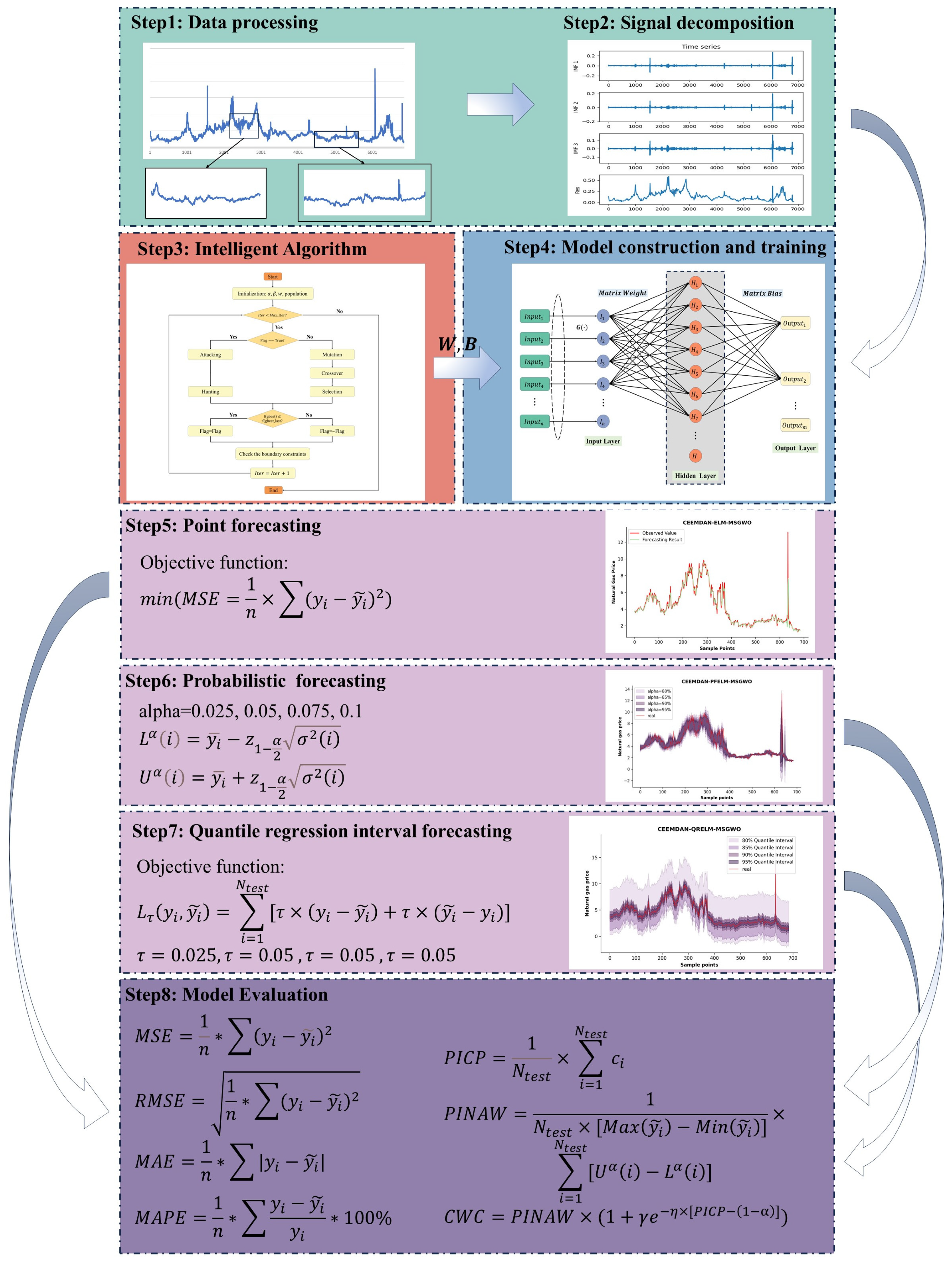
4. Forecasting Framework

As shown in Figure 3, the proposed forecasting framework comprises eight major components: data preprocessing, signal decomposition, optimization algorithm, predictor, point forecasting, probability interval forecasting, quantile interval forecasting, and model evaluation.

4.1. Data Preprocessing

Natural gas prices are derived from market transaction records; however, these records often contain noise and outliers. These noises and outliers can result from statistical errors, system failures, and other external factors. Therefore, effective preprocessing of the data to remove or smooth out these outliers is critical for improving the predictive model. In addition, missing values may occur in the natural gas price series. Commonly used missing value processing methods include interpolation, nearest neighbor, and regression methods. Additionally, ELM models typically require input variables to have values between 0 and 1 or between −1 and 1. Through normalization, the natural gas price series can be scaled to values between 0 and 1. The benefit of normalization is that the ELM model can be trained correctly, and the optimization algorithm will perform better because the values of the different features remain similar and more consistent with the model’s assumptions. This process allows the model to capture trends in the price series more accurately and improve the forecasting results.

4.2. Decomposition of Natural Gas Price Series

Signal decomposition plays a pivotal role in the field of TSF, and its importance and far-reaching impact should not be underestimated. Through signal decomposition, complex data structures can be effectively separated into simple data patterns, facilitating an in-depth study of the trends. Thus, the prediction model is better able to capture specific patterns in the data. At the same time, signal decomposition techniques improve the robustness and accuracy of the prediction model by removing noise, smoothing the data, and extracting features.

EEMD is a widely used signal-processing technique. It introduces Gaussian white noise into the process, and by averaging the decomposition results several times, it can effectively mitigate the modal aliasing issue because of noise. At the same time, by averaging these IMFs, the EEMD can improve the structural separation and remove the added white noise. Applying EEMD to time series data can enhance the adaptability and accuracy of forecasting models.

4.3. Optimization Algorithm

The proposed MSGWO was used to determine the most suitable ELM hidden layer matrices to improve the prediction model. There are two hidden layer matrices in the ELM, which are known as matrix $w$ and matrix $b$. $w$ is the weight matrix, which denotes the weights from the input layer to the hidden layer and is used to control the mapping process. The choice of the column number of the matrix $w$, which corresponds to the neuron number, affects the capacity of the model: if the capacity is too small, it may not be able to capture complex relationships from the data, whereas too large a capacity may lead to overfitting. Conversely, the number of rows of the matrix $w$ corresponds to the number of features in the input data and controls the fitting process. The matrix $b$ represents the bias matrix of the hidden layer, also known as the hidden layer bias term. Matrix $b$ introduces a nonlinear transformation so that the output contains nonlinear information. The size of the matrix $b$ affects the degree of nonlinearity introduced. Appropriate nonlinear transformations help improve the fit of the model and capture the complex relationships between the data. The greater the number of bias terms, the greater the flexibility; however, it can also lead to overfitting. Correct fitting requires a balance between the model fit and generalizability. When training the model, the main implementation of ELM is to adaptively adjust the size of the $w$ and $b$ matrices to gradually reduce the difference between the output and the training target in order to achieve a good fit. Matrix $w$ and matrix $b$ have a significant impact on the adaptability and generality of the model, so the optimization targets are matrix $w$ and $b$.

Assuming that the vector $x$ is the decision variable of optimization, $x$ can be expressed by Equation (22):

$$x=(w,b)$$

(22)

where $w$ denotes the weight matrix, and $b$ denotes the bias matrix. The search range of matrix $w$ and matrix $b$ is shown in

Table 2. Table of Hyperparameters.

Hyperparameters	Search Scope	Role of the Hyperparameter
$w$	$[-1,1]$	Controlling the mapping process to influence feature extraction.
$b$	$[-1,1]$	Introduce nonlinearity to enhance the representativeness of the model.

:

4.4. Predictor

The learning speed of ELM is extremely fast. Compared with traditional iterative learning methods, ELM usually learns more efficiently because the output layer weights can be computed directly from the parsing solution. In practice, ELM exhibits good generalization performance, especially on large datasets. Therefore, this paper uses ELMs as predictors. Each IMF is divided into two parts: the training and testing parts. The training data were used to tune the model and optimize the hidden layer matrices, whereas the test data were used to measure the performance of the predictive model.

4.5. Point Forecasting

Point forecasting is an important analytical technique in time-series forecasting. The purpose of point forecasting is to analyze historical data to capture patterns to estimate values at a specific point in time in the future. In the case of natural gas price forecasting, the primary objective of point forecasting is to accurately capture future trends in the natural gas market prices. Natural gas produces relatively little carbon dioxide and other air pollutants from combustion as a clean energy source, helping to combat climate change and improve air quality compared to other energy sources. Point-to-point forecasting results not only help companies and governments make real-time decisions but also provide stakeholders in the natural gas market with price trends, thereby facilitating informed decisions on trade and investment in the natural gas industry and promoting sustainable development and the development of a low-carbon economy in the natural gas sector. Forward-looking forecasts provide a more intuitive understanding of future natural gas price trends and provide a scientific basis for achieving carbon reduction targets.

The developed forecasting framework adopts the Mean Squared Error (MSE) metric, defined in Equation (23), to quantify the prediction accuracy and guide parameter optimization.

$$min(MSE={\displaystyle \frac{1}{n}}\times \sum {(y_i-\widetilde{y_i})}^2)$$

(23)

where $y_i$ denotes the $i$th actual observation, $\widetilde{y_i}$ is the $i$th output, and $n$ is the sample size.

4.6. Probability Interval Forecasting

Probability-interval forecasting can provide more comprehensive information. By introducing probability distributions, the method not only predicts individual sample points but also provides probabilistic estimates of possible future trends in natural gas price volatility. The advantage of the probability interval forecasting method is that it captures the uncertainty of market fluctuations and provides diversified support to decision-makers in the presence of uncertainty.

Assume that the time series $Y=(y_1,y_2,y_3,\cdots ,y_n)$, where the sample number is $n$. The data is randomly and putatively sampled $B$ times ($B\ge 10$) using the Bootstrap method, and each time, $m$ observations ($m\le n$) are extracted. The Bootstrap sampling samples are then reordered according to the serial numbers of the extracted observations in the original series to form a dataset containing $B$ Bootstrap samples about the time series $Y$, so that the nature and distribution of the time series $Y$ can be further investigated. The specific steps of the probability interval forecasting model of natural gas price based on the Bootstrap method are as follows:

Step 1: Obtain the original sample dataset $Y=\left(y_1,y_2,y_3,\cdots ,y_n\right)$ of natural gas trading prices, where $n\in N^{+}$.

Step 2: Resampling. Draw $m$ ($m\in N^{+},m\le n$) samples from the natural gas price time series $Y$ randomly and with a putback, and at the same time construct the first Bootstrap sample $Y_1^{\ast }=\left(y_1^{\ast },y_2^{\ast },y_3^{\ast },\cdots ,y_m^{\ast }\right)$ by arranging the drawn samples according to their ordinal numbers from smallest to the largest in the original sample Y. Repeat the extraction of $B$ ($B\in N^{+}$) times to get Bootstrap sample set $Y^{\ast }=(Y_1^{\ast },Y_2^{\ast },Y_3^{\ast },\cdots ,Y_B^{\ast })$.

Step 3: Construct a point prediction model. Divide each sample in the Bootstrap sample set $Y^{\ast }$ into training and test sets, and input the training sets to the point forecasting model to obtain $B$ point forecasting models.

Step 4: Model Prediction. The prediction model obtained in Step 3 is used to conduct prediction experiments on the test set of $B$ Bootstrap samples respectively, and the set of $B$ prediction sequences $\tilde{Y}=\widetilde{Y_1^{\ast }},\widetilde{Y_2^{\ast }},\widetilde{Y_3^{\ast }},\cdots ,\widetilde{Y_B^{\ast }}$ is obtained.

Step 5: Construct probability forecasting intervals. After step 4, a sequence set $\tilde{Y}=\widetilde{Y_1^{\ast }},\widetilde{Y_2^{\ast }},\widetilde{Y_3^{\ast }},\cdots ,\widetilde{Y_B^{\ast }}$ can be obtained, which consists of the predicted results of the group of points in group $B$, where $j$th predicted sequence set $\widetilde{Y_j^{\ast }}=\left(\widetilde{y_{j1}^{\ast }}, \widetilde{y_{j2}^{\ast }},\widetilde{y_{j3}^{\ast }},\cdots ,\widetilde{y_{jk}^{\ast }}\right),k=0.1\times m$. In the set of prediction sequences $\tilde{Y}$, for the $i$th sample point, there are a total of $B$ predicted values, which can form the sequence $\widetilde{Y_i^{\ast }}={\left(\widetilde{y_{1i}^{\ast }},\widetilde{y_{2i}^{\ast }},\widetilde{y_{3i}^{\ast }},\cdots ,\widetilde{y_{Bi}^{\ast }}\right)}^T$. The computation leads to the mean value of the sequence $\widetilde{Y_i^{\ast }}$ as $\overline{y_i}$, and variance as ${\sigma }^2\left(i\right)$. Assuming that the confidence level is $100\times (1-\alpha )\%$, the probability forecasting interval $I$ for $y_i$ can be expressed by Equation (24):

$$I^{\alpha }\left(i\right)=[L^{\alpha }\left(i\right),U^{\alpha }\left(i\right)]$$

(24)

where $I^{\alpha }\left(i\right)$ denotes the probability forecasting interval when the confidence is $100\times (1-\alpha )\%$, $L^{\alpha }\left(i\right)$ and $U^{\alpha }\left(i\right)$ denote the lower and upper limits of the $i$th probability forecasting interval, respectively, and $i$ is the ordinal number of the forecasting target. Equation (24) makes the interval coverage $P\left(\widetilde{y_i}\in I^{\alpha }\right)=100\times \left(1-\alpha \right)\%$. $L^{\alpha }\left(i\right)$ and $U^{\alpha }\left(i\right)$ can be calculated by the following method:

$$L^{\alpha }\left(i\right)=\overline{y_i}-z_{1-{\displaystyle \frac{\alpha }{2}}}\sqrt{{\sigma }^2\left(i\right)}$$

(25)

$$U^{\alpha }\left(i\right)=\overline{y_i}+z_{1-{\displaystyle \frac{\alpha }{2}}}\sqrt{{\sigma }^2\left(i\right)}$$

(26)

where $L^{\alpha }\left(i\right)$ and $U^{\alpha }\left(i\right)$ are the lower and upper boundaries of the $i$th probability forecasting interval, $\overline{y_i}$ denotes the mean of the $B$ point forecasted values obtained by the prediction of the $i$th observation, ${\sigma }^2\left(i\right)$ is the variance of the $B$ point predicted values obtained by the prediction of the $i$th observation, and $z_{1-{\displaystyle \frac{\alpha }{2}}}$ denotes the standard Gaussian distribution’s critical value at $100\times (1-\alpha )\%$ confidence level. When the boundary of $I^{\alpha }\left(i\right)$ exceeds $[0,1]$, it will be adjusted to the lower or upper boundary.

4.7. Quantile Interval Forecasting

In natural gas price forecasting, interquartile range forecasting is an important method for providing more information about uncertainty. By introducing the concept of the interquartile range, this methodology not only focuses on the central tendency but also illustrates the range of natural gas price changes. With interquartile range forecasting, policymakers can gain a more comprehensive understanding of the likelihood of natural gas price volatility and implement adaptive risk governance protocols to enhance strategic responsiveness in exposure control. Interquartile range forecasts are better able to cope with outliers and noise because they do not rely too heavily on a single data point but rather take into account the entire forecast horizon.

4.7.1. Quantile Loss Function

A commonly used objective function for interquartile range forecasting is the quantile loss function, which is intended to model tail risk more completely when forecasting different quantiles. Unlike the objective function for point forecasting models, the quantile loss function does not minimize the total squared errors but rather minimizes the total absolute errors arising from the selected quantile cut points. A commonly used loss function formulation is the pinball loss [51]. Pinball loss is characterized by directing the focus of the model to the already defined range of quantile values by adjusting the penalty for prediction errors at different quantile values. The mathematical expression for the quantile loss function is as follows:

$$Quantile Loss(\tau )={\displaystyle \frac{1}{N}}\times {\sum }_1^{N}loss$$

(27)

where $Quantile Loss\left(\tau \right)$ is the quantile forecasting loss in model training, $\tau$ is the value of the selected quantile, $N$ is the sample size, and $loss$ denotes the quantile loss for each prediction target, which can be obtained by using Equation (28).

$$loss=\left\{\begin{array}{c}\tau \times |y_i-\widetilde{y_i}|\\ \left(1-\tau \right)\times |y_i-\widetilde{y_i}|\end{array}\right.\begin{array}{c},y_i>\widetilde{y_i}\\ ,y_i\le \widetilde{y_i}\end{array}$$

(28)

where $loss$ denotes the quantile loss for each prediction target, $\tau$ is the selected quantile value, $y_i$ denotes the $i$th observation, and $\widetilde{y_i}$ denotes the $i$th quantile forecasting value.

In Equations (27) and (28), $\tau \times |y_i-\widetilde{y_i}|$ is the loss when the forecasted value is smaller than the observation, and $\left(1-\tau \right)\times |y_i-\widetilde{y_i}|$ denotes the lagers. Through considering different $\tau$ values, this function can be further understood as follows:

(1)

When $\tau =0.5$, the forecasted value is smaller or larger than the observed value with equal weights. In this situation, the loss function is the same as the Mean Absolute Error (MAE).

(2)

When $\tau >0.5$, the loss weights are higher when the forecasted value is smaller than the observation. To minimize the loss, the model tends to make the forecasting values relatively large. This contributes to a relative increase in the predicted value, which can be interpreted as obtaining the upper boundary of the quantile forecasting interval.

(3)

When $\tau <0.5$, the weight of loss is higher when the forecasted result is larger. At this point, the goal of the model is to adjust the forecasted result to be relatively small in order to minimize the loss. This results in a relatively lower predicted value, which can be interpreted as being used to determine the lower limit of the interquartile prediction interval.

4.7.2. Construction of Quantile Forecasting Interval

In practice, quantile interval forecasting often specifies several different quantile values to fully measure the effectiveness of the quantile interval forecasting model. By adjusting the hyperparameter $\tau$, an error threshold can be chosen that is appropriate for balancing the problems that need to be solved. The output corresponding to each quantile $\tau$ is a complete but biased point prediction result. By using the prediction results of quartile $\tau$ and quartile $1-\tau$ as the lower and upper boundaries, respectively, a quartile forecasting interval with a confidence level of $(1-2\tau )\times 100\%$ can be constituted.

4.8. Criterions for Evaluation

4.8.1. Evaluation of Point Forecasting

In this study, four commonly used criteria are set to evaluate the point-forecasting models. First, the MSE is used as a variance measure. The MSE is defined as follows:

$$MSE={\displaystyle \frac{1}{n}}\times \sum {(y_i-\widetilde{y_i})}^2$$

(29)

where $y_i$ is the observation, $\widetilde{y_i}$ is the prediction result, and $n$ is the sample size.

Second, the Root Mean Square Error (RMSE) was chosen as a performance criterion, which is defined as follows:

$$RMSE=\sqrt{{\displaystyle \frac{1}{n}}\times \sum {(y_i-\widetilde{y_i})}^2}$$

(30)

where $y_i$ is the observation, $\widetilde{y_i}$ is the forecasting result, and $n$ is the sample size.

Third, the MAE is used as the accuracy criterion and is defined as follows:

$$MAE={\displaystyle \frac{1}{n}}\times \sum |y_i-\widetilde{y_i}|$$

(31)

where $y_i$ is the observation, $\widetilde{y_i}$ is the prediction result, and $n$ denotes the sample size.

Finally, the Mean Absolute Percentage Error (MAPE) is selected to measure the relative error in natural gas price point forecasting and is represented as follows:

$$MAPE={\displaystyle \frac{1}{n}}\times \sum {\displaystyle \frac{y_i-\widetilde{y_i}}{y_i}}\times 100\%$$

(32)

where $y_i$ is the observation, $\widetilde{y_i}$ is the prediction result, and $n$ denotes the sample size.

4.8.2. Evaluation of Probability and Quantile Interval Forecasting

Given the bands of continuous-value uncertainty generated by interval forecasting, the traditional point prediction evaluation paradigm is inappropriate for evaluating interval-based prediction results. In order to rigorously quantify the reliability and accuracy of these interval forecasting methods, we selected three evaluation criteria, each targeting a different aspect of the interval prediction performance.

The first metric is Prediction Interval Coverage Probability (PICP). $PICP$ calculates the probability that an actual observation falls within the prediction interval, and it’s calculated as in Equations (33) and (34), as follows:

$$PICP={\displaystyle \frac{1}{N_{test}}}\times \sum _{i=1}^{N_{test}}{c}_i$$

(33)

where $N_{test}$ denotes the sample size and $c_i$ denotes the coefficient of 0 or 1. $c_i$ can be calculated using Equation (34), as follows:

$$c_i=\left\{\begin{array}{c}1, \\ 0, \end{array}\right.\begin{array}{c}{y}_i\in I_t^{\alpha }\left(i\right)\\ y_i{\notin I}_t^{\alpha }\left(i\right)\end{array}$$

(34)

where $y_i$ is the $i$th observation, and $I_t^{\alpha }\left(i\right)$ is the interval corresponding to the $i$th observation at a confidence level of $100\times (1-\alpha )\%$ as calculated by the probability interval forecasting model and the quantile interval forecasting model.

The next indicator is the Prediction Interval Normalized Average Width (PINAW), which is the ratio of the mean value of the width of the forecasting intervals to the standard deviation of the actual observations. The formula for $PINAW$ is Equation (35).

$$PINAW={\displaystyle \frac{1}{N_{test}\times \left[{\sigma }^2\right(Y\left)\right]}}\times \sum _{i=1}^{N_{test}}[U^{\alpha }\left(i\right)-L^{\alpha }\left(i\right)]$$

(35)

where $U^{\alpha }\left(i\right)$ and $L^{\alpha }\left(i\right)$ denote the upper and lower boundaries, respectively, ${\sigma }^2\left(Y\right)$ is the variance of the test data, and $N_{test}$ denotes the sample number.

In the realistic forecasting process, the phenomenon of relatively high coverage of intervals but a relatively large average width of intervals often occurs. In this case, we chose the last evaluation metric, the Calibration Width Coverage (CWC). The smaller $CWC$ means the better effectiveness. Equation (36) defines the calculation method of $CWC$.

$$CWC=PINAW\times (1+\gamma e^{-\eta \times [PICP-\left(1-\mathsf{\alpha }\right)]})$$

(36)

where $PINAW$ is derived from Equation (35), $PICP$ is derived from Equation (33), $\gamma$ is used to penalize models that do not meet preset coverage, $e$ is the natural constant, and $\eta$ is an exponential function that serves to amplify the penalization of models that do not meet the preset coverage, which is usually set to 40, $1-\alpha$ denotes the confidence level for calculating probability forecasting intervals and the quantile level for calculating quantile forecasting intervals. $\gamma$ can be calculated using Equation (37):

$$\gamma =\left\{\begin{array}{c}1,\\ 0, \end{array} \right.\begin{array}{c}PICP<(1-\alpha )\\ otherwise\end{array}$$

(37)

where $PICP$ is calculated using Equation (33), $1-\alpha$ denotes the confidence level.

5. Point Forecasting Experiments

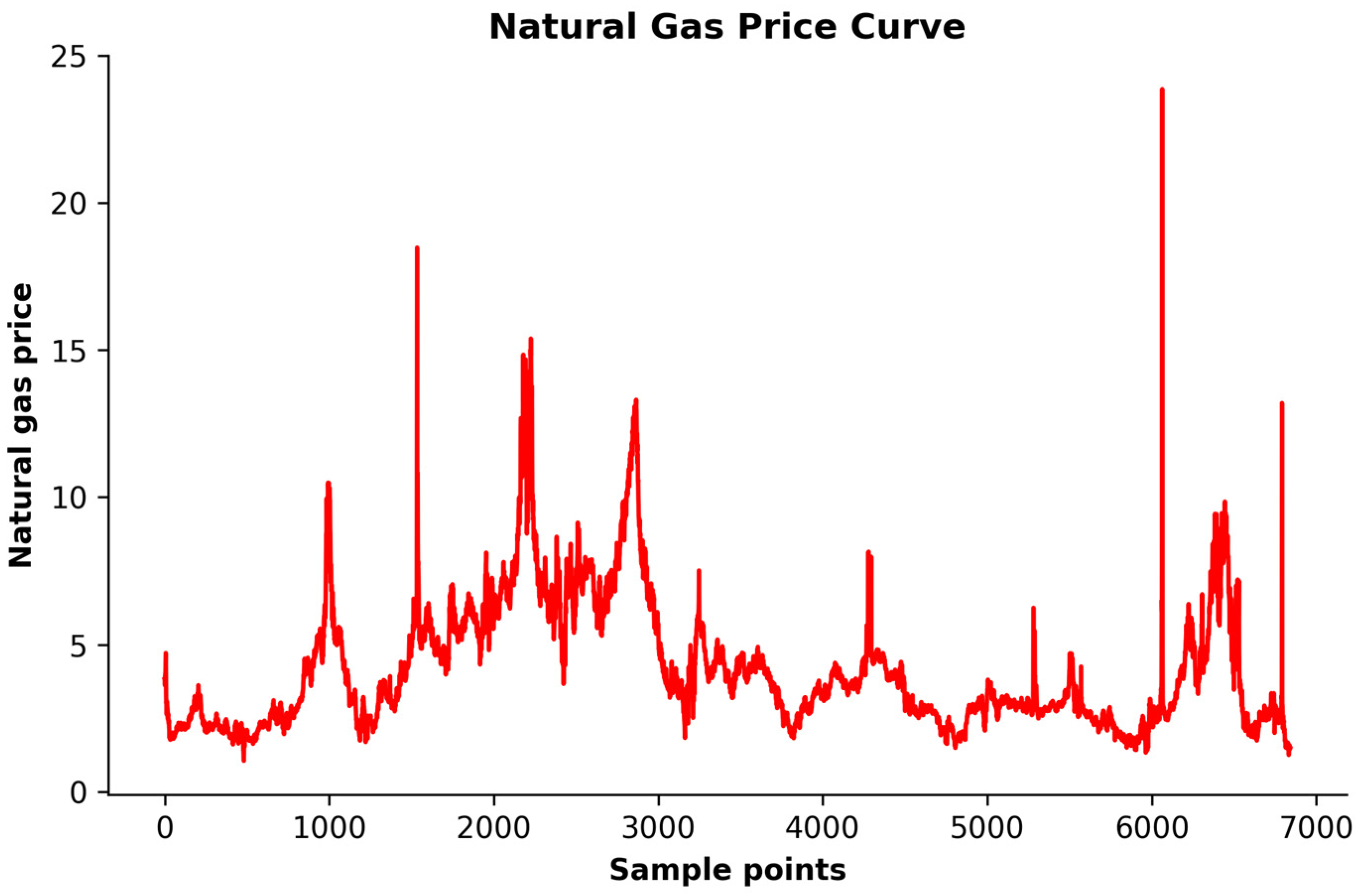
5.1. Research Data and Experimental Setting

This research uses daily natural gas prices from the U.S. Energy Information Administration for this experiment. The experimental data covers natural gas trading prices from 7 January 1997 to 26 March 2024, with a total of 6843 samples. A line graph of the observation data is shown in Figure 4.

Before the forecasting experiment begins, the natural gas price time series is first preprocessed to correct and fill in outliers and missing values by interpolation. The preprocessed series are then normalized to the range of −1 to 1 to prevent the gradient from disappearing and to meet the input requirements of the ELM. The sequences are split into the training and test sets.

Table 3. Data composition table of the dataset.

Sample Size	Training Set (Size)	Test Set (Size)
6843	7 January 1997–30 June 2021 (6158)	1 July 2021–26 March 2024 (685)

shows the series division.

All experiments are conducted under identical conditions using Python 3.9 programming language, a laptop with an Intel Core i7, 3.4 GHz CPU, and 20 GB of RAM, and an operating system of Windows 10.

5.2. ELM with Optimization Algorithms

Although ELM shows great potential for natural gas price forecasting, several challenges persist, particularly in optimizing its hyperparameters. The predictive performance of ELM is highly sensitive to the selection of key parameters, such as synaptic connection weights and bias vectors, which significantly influence the model’s effectiveness.

By employing intelligent optimization algorithms to tune the model’s hyperparameters, the model can be more effectively adapted to varying data characteristics, thereby enhancing its robustness and generalization capability. Optimizing the hyperparameters enables the model to better exploit the intrinsic information contained in the data, ultimately improving its predictive performance for natural gas price forecasting.

In the first part, different optimization algorithms are used to identify the optimal hidden layer matrices for the ELM. Six metaheuristic-driven algorithms—GWO [29], DE [52], PSO [53], Moth-Flame Optimization (MFO) [54], WOA [55], and our novel MSGWO are implemented to refine synaptic connection weights and bias vectors through iterative parameter space navigation. Reconstructed ELM variants with evolutionarily optimized neural topologies are subsequently deployed for natural gas price forecasting. The experimental controls incorporate baseline ELM implementations without parametric enhancement. Each configuration undergoes decuple Monte Carlo realizations ($N=10$) under identical computational constraints to ensure statistical robustness. Additionally, we selected XGBOOST, Long Short-Term Memory (LSTM), Convolutional Neural Networks (CNN), Temporal Convolutional Networks (TCN), and transformer models for comparison with ELM to validate the rationale behind choosing ELM as the forecasting model. The prognostic performance metrics are aggregated through ensemble averaging, and the comprehensive quantitative evaluation is presented in

Table 4. Statistical table of point forecast results (ELM-Algorithm).

Model	MSE	RMSE	MAE	MAPE
ELM	0.3641	0.6034	0.3017	7.1425
XGBOOST	0.4330	0.6580	0.3516	9.6455
LSTM	0.4687	0.6846	0.3391	8.0089
CNN	2.0780	1.4415	1.0395	20.2005
TCN	0.6146	0.7840	0.5170	11.8156
Transformer	0.5164	0.7186	0.4962	14.9419
ELM-GWO	0.3662	0.6051	0.2434	5.6664
ELM-DE	0.3651	0.6042	0.2443	5.7236
ELM-PSO	0.3642	0.6035	0.2404	5.6370
ELM-MFO	0.3536	0.5946	0.2411	5.6363
ELM-WOA	0.3687	0.6072	0.2421	5.6205
ELM-MSGWO	0.3626	0.6021	0.2387	5.5991

. The forecasting results of the MSGWO-enhanced ELM framework are further visualized in Figure 5, demonstrating superior market pattern tracking fidelity.

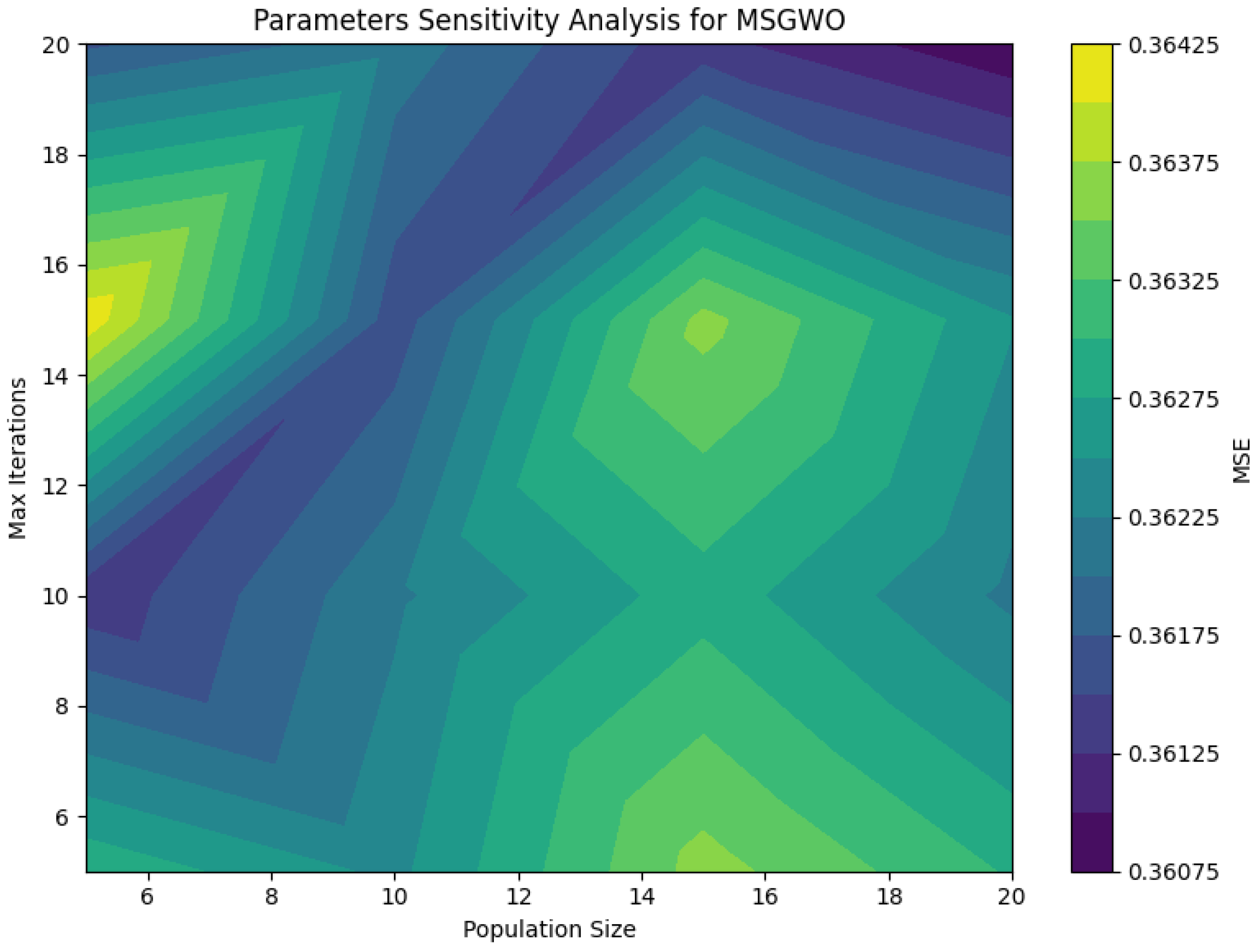
Moreover, to assess the stability of the model, we analyzed the impact of the population size and number of iterations on the prediction accuracy of MSGWO. Both parameters were set to 5, 10, 15, and 20, and the corresponding model performance was evaluated. The results are shown in Figure 6. The model exhibits stable performance across different parameter configurations, with relatively minor variations in prediction accuracy. Considering the trade-off between predictive performance and computational complexity, both the population size and the number of iterations were set to 10.

By comparing the statistical metrics of the ELM and the models optimized using swarm intelligence mechanisms in Table 4, the following conclusions can be drawn.

First, the parametric refinement of the hidden layer matrices through metaheuristic-driven optimization frameworks demonstrated measurable improvements in the predictive fidelity of the ELM. The direct forecasting results using the traditional ELM model reached an acceptable level: the MAPE metrics for the forecasting results of the ELM reached 6.6740%, which indicates that ELM has good performance on the accuracy and generalization aspects still have much room for improvement. In particular, when processing non-stationary signals exemplified by natural gas price series, the ELM faces significant bottlenecks in capturing deeper factors. To solve these problems, our methodology integrates evolutionary computation paradigms for the parametric refinement of the synaptic architecture of the ELM. Each evolutionary strategy implements probabilistic search operators, including gradient-free exploration and adaptive mutation heuristics, to systematically calibrate the neural projection matrices. This optimization framework facilitates hierarchical feature abstraction from non-stationary temporal patterns, enabling comprehensive latent variable discovery. Empirical validation demonstrates marked improvements in prognostic capability across all benchmark metrics. The metaheuristic-enhanced ELM variants exhibit superior nonlinear fitting capability, confirming their enhanced capacity for multi-scale pattern recognition in complex energy market dynamics.

Second, the proposed MSGWO exhibits superior overall performance compared with other intelligent optimization algorithms. The MSGWO reached the minimum values in MAE and MAPE and consistently maintained the top performance in MSE and RMSE, ranking second. This not only highlights the excellent performance of the MSGWO in hidden layer parameter finding for ELM but also proves its advantages in helping predictive models capture data features and fit the models. A granular examination of the MSGWO demonstrated that its innovative exploration dynamics and swarm-based metaheuristic framework significantly enhance the parameter optimization capabilities in ELM. The MSGWO emulates social dynamics encompassing wolves, both cooperative pack behavior and individual dominance hierarchies, and simultaneously employs three strategies, namely, mutation, crossover, and selection, to refine the shortcomings of the GWO in navigating high-dimensional search spaces. The mutation strategy greatly improves the group diversity. In contrast, the crossover strategy accelerates the optimization process and facilitates a global search. This selection strategy is conducive to improving the convergence speed and stability. The addition of these three strategies enables the MSGWO to maintain an adaptive equilibrium between exploration-exploitation tradeoffs, which improves the search efficiency, better avoids premature convergence, and achieves remarkable results in the optimization process of ELM’s synaptic connection parameters.

5.3. Decomposition of Natural Gas Price Time Series

In this section, we perform signal decomposition operations on the natural gas price series and conduct a second round of experiments. A methodologically rigorous comparison of temporal decomposition techniques is conducted to quantify their influence on predictive performance by evaluating four principal approaches: EMD [56], CEEMDAN [57], Variational Mode Decomposition (VMD) [58], and EEMD [46].

It is known from existing studies that the performance of decomposition techniques is more susceptible to two key parameters: the ensemble iteration count $n$ and the Gaussian-distributed perturbation magnitude $\epsilon$ [59]. As formalized in Wu and Huang’s canonical statistical framework in Equation (38), the selection of the above parameters has a large correlation with the standard deviation of the error $e_n$ [46]. Theoretical analyses establish that stochastic perturbations exhibit a scaling behavior governed by the mathematical framework in Equation (38). Empirical evaluations across multiple trials have demonstrated an optimal perturbation magnitude of approximately 0.2 times the empirical standard deviation in observational datasets. Complementary investigations by Zhang et al. into the parametric configuration in ensemble decomposition methodologies yielded experimental validation that corroborated the theoretical congruence initially posited in foundational studies [60].

$$e_n={\displaystyle \frac{\epsilon }{\sqrt{n}}}$$

(38)

where $e_n$ denotes the population standard deviation, $\epsilon$ specifies the Gaussian-distributed perturbation magnitude, and $n$ indicates the total iteration cycles in the ensemble process.

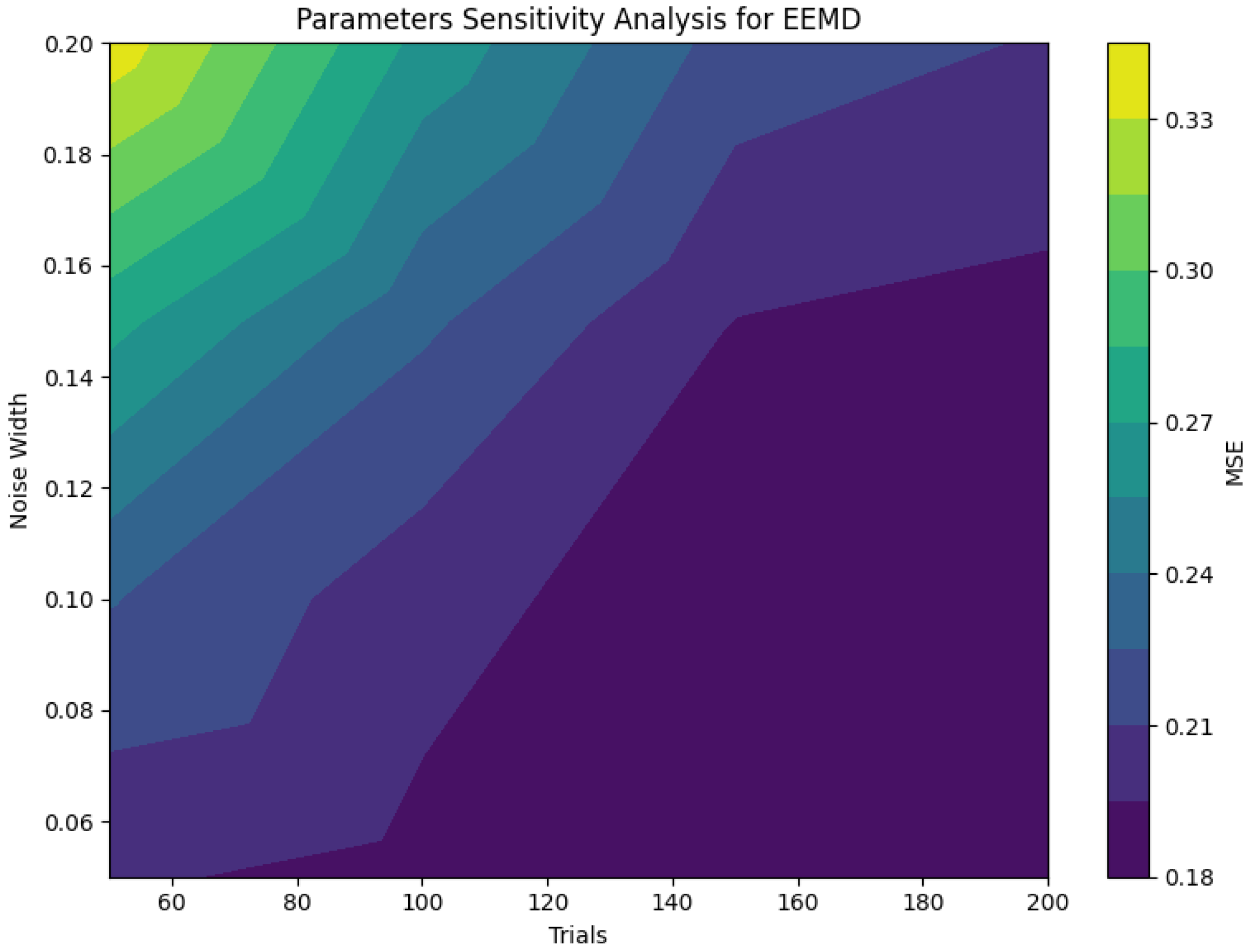
Parametric influence mechanisms are comprehensively addressed in the foundational work of Wu and Huang, to which readers are directed for methodological details. To verify the sensitivity of the EEMD to its parameters, we analyzed two key factors: the noise amplitude and the number of ensemble iterations. Specifically, the noise amplitudes were set to 0.05, 0.1, 0.15, and 0.2, while the number of ensemble iterations was set to 50, 100, 150, and 200. The corresponding variation in the MSE was observed to assess the impact of these settings, and the experimental results are presented in Figure 7.

It is evident that the prediction accuracy deteriorates as the noise amplitude increases, while it improves with a higher number of ensemble iterations. To ensure the generalization ability of the model and avoid overfitting and underfitting, we refer to the parameter settings recommended in previous studies for guidance. Our implementation employs an ensemble-based modal decomposition methodology configured with 100 iteration cycles and a Gaussian noise component magnitude scaled to 0.05 times the signal’s standard deviation. 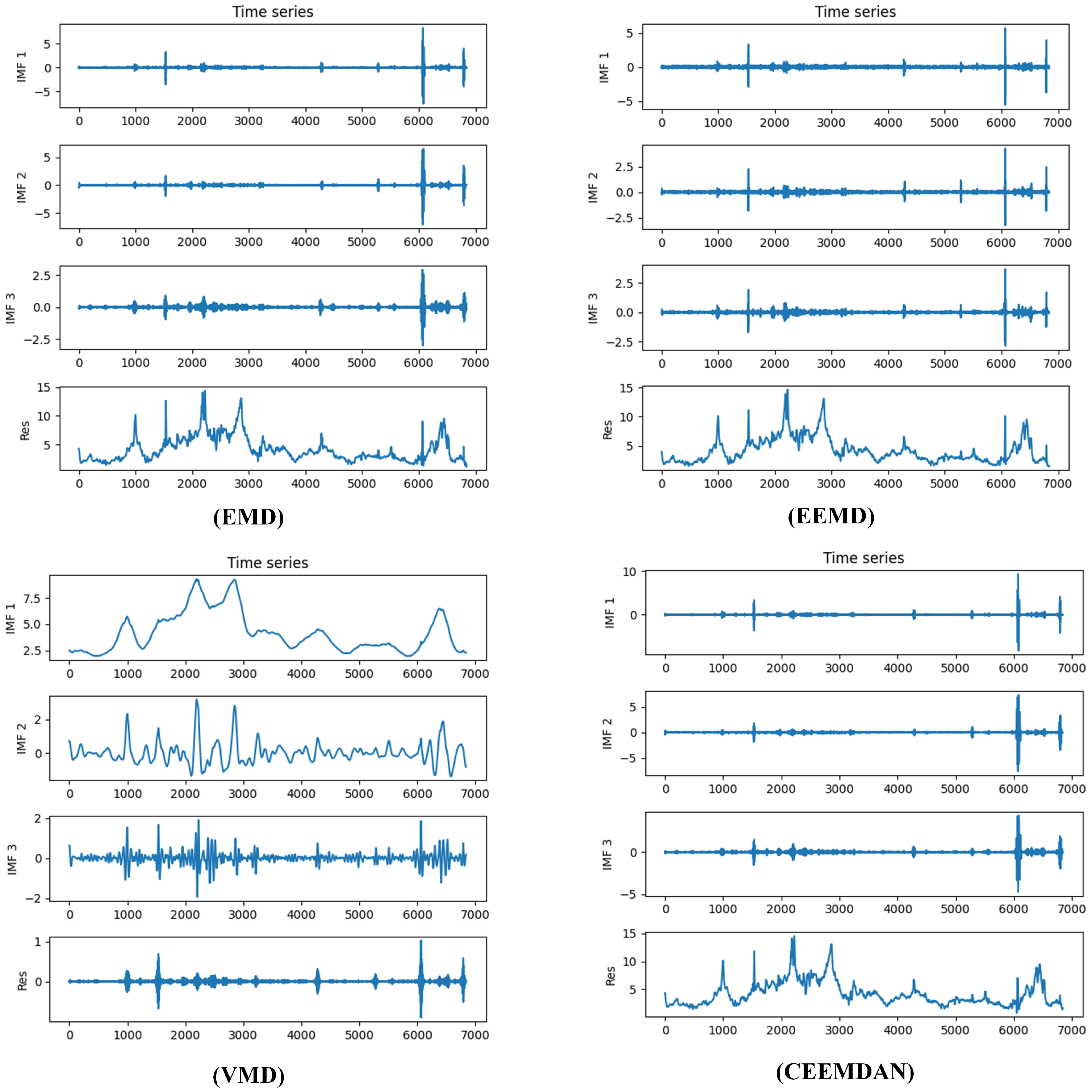Figure 8 illustrates the application of four distinct decomposition approaches to the natural gas price series, demonstrating the characteristic mode separation capabilities.

5.4. ELM with Decomposition Methods

By analyzing the natural gas price data in both the time and frequency domains, we argue that the IMF components extracted through decomposition effectively capture the key dynamic features of the time series. Specifically, IMF1 reflects high-frequency fluctuations or noise, representing short-term oscillations in natural gas prices. IMF2 captures medium-term cyclical patterns and seasonal variations, while MF3 primarily represents low-frequency components that correspond to long-term trends. These decomposition techniques not only offer a more nuanced understanding of price volatility across different time scales but also provide more structured and informative inputs for subsequent modeling and forecasting tasks.

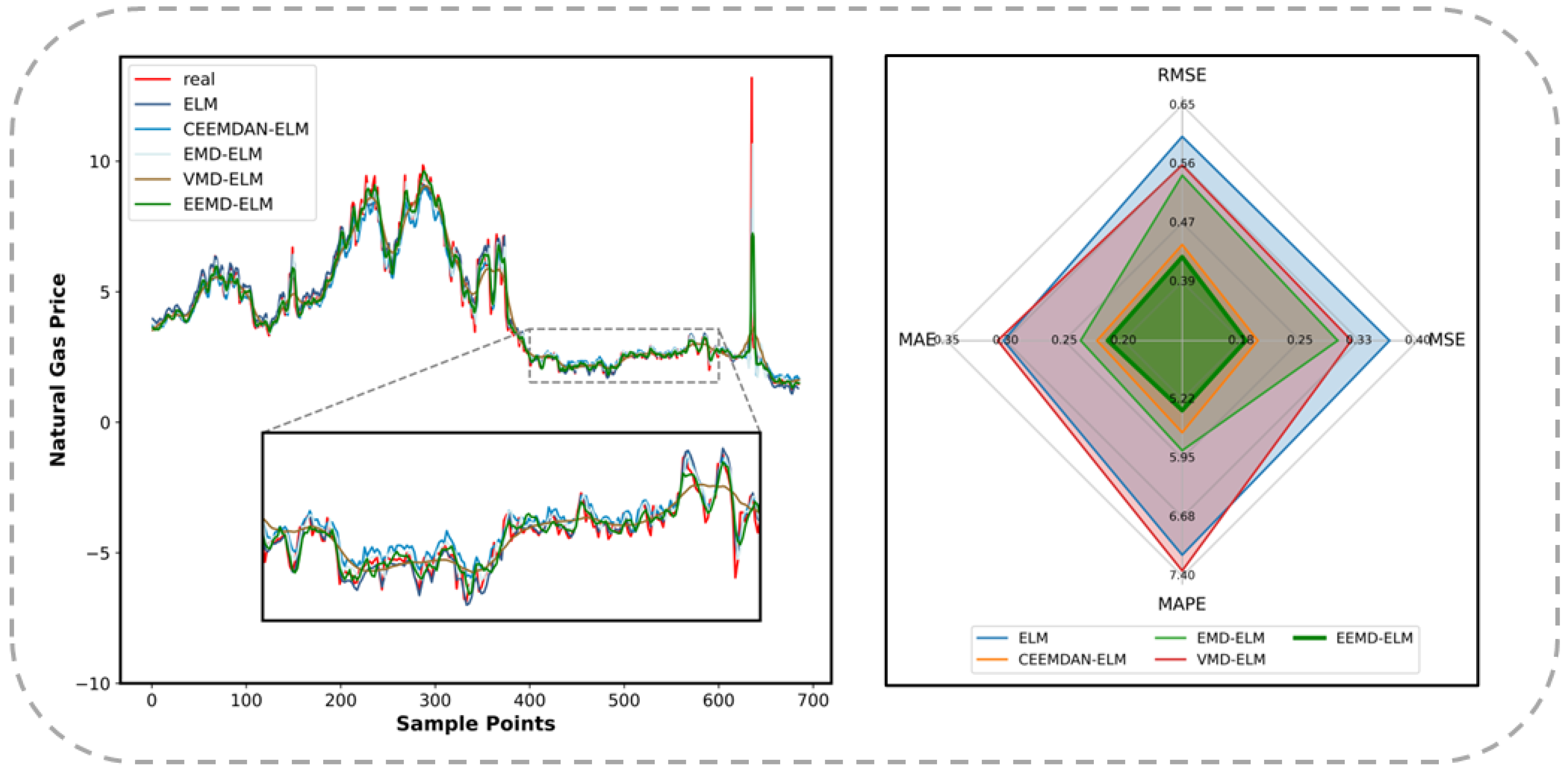
To assess the effectiveness of various signal decomposition techniques in decomposing the natural gas price time series and their impact on the ELM model, we compare and analyze forecasting models that incorporate these techniques. We first decompose the series using each of the techniques described above, as described in Section 5.3. In the next step, the obtained IMFs and residuals were split into training and test sets. Using the training sets as input to the ELM model, forecasting models corresponding to different IMFs can be trained, which in turn yields forecasting results corresponding to each IMF and residual. After accumulating the sets of forecast results correspondingly, the point forecasting results can be obtained. In the experiments of the forecasting models with the addition of the signal decomposition techniques, the same 10 experiments were carried out independently for each of these models, and the mean values of the same metrics obtained were calculated. The quantified performance metrics for all experimental configurations are systematically presented in

Table 5. Statistical table of point forecast results (Decomposition-ELM).

Model	MSE	RMSE	MAE	MAPE
ELM	0.3641	0.6034	0.3017	7.1425
CEEMDAN-ELM	0.1963	0.4426	0.2223	5.6331
EMD-ELM	0.2980	0.5457	0.2362	5.8553
VMD-ELM	0.3154	0.5611	0.3067	7.3370
EEMD-ELM	0.1810	0.4243	0.2131	5.3607

. Complementary to the tabular data, the prognostic outputs of the EEMD-ELM are visualized through a line graph, as shown in Figure 9.

As displayed in Table 5, the ELM forecasting model based on EEMD has the most accurate and highest coincidence results for the natural gas price series, surpassing the predictions by models applying other decomposition methods. Further analysis of the various statistical indicators enables the formulation of the following principal findings:

First, the pre-decomposition of time series has been found to positively contribute to the improvement of the accuracy of the forecasting results. Significant decreases in all four statistical indicators have been shown in the results of the forecasting models that apply the EMD, CEEMDAN, and EEMD methods. The significant reductions in the above indicators indicate that the accuracy of the prediction models has notably improved, representing the positive impact of signal processing techniques on prediction accuracy in time series forecasting. Time series data are typically composed of multiple components with different scales and frequencies, such as secular tendencies, seasonal variations, and high-frequency noise. By decomposing the time series, the components of different scales can be separated, making the characteristics of each component more distinct. In this way, the decomposed sequences, with noise and redundant information removed, become easier to interpret, allowing the true patterns within the data to be more accurately captured by forecasting models. Consequently, the predictive capability of the models is enhanced by the decomposition techniques. The ELM model incorporating the VMD technique showed improvements in MSE and RMSE compared to the original ELM. However, weaker performance was observed in MAE and MAPE, which may be attributed to inaccuracies in feature extraction or information loss, among others. If the signal is overly complex, containing multiple frequency components with mutual interactions, the signal might fail to be accurately decomposed into distinct modes by VMD, which can lead to inaccurate features being extracted and affect the prediction of the ELM model. From this, it can be seen that not all signal decomposition methods are suitable for all the time series. For the natural gas price series, VMD evidently cannot clearly distinguish between important information and noise, resulting in the ELM model being unable to learn sufficiently effective features.

Second, the decomposition effect of the EEMD technique surpasses that of other decomposition methods. Among the original ELM model and the four models incorporating signal decomposition techniques, the EEMD-ELM achieved the most optimal prediction results. For RMSE and MAE, the EEMD-ELM model demonstrated a reduction of more than 20% compared to ELM, the optimization margin in MSE exceeded 45%, and an improvement of nearly 20% was also achieved in MAPE. These optimization margins significantly surpassed those of other decomposition methods, demonstrating the superiority of the EEMD. As a multi-scale signal decomposition method, EEMD can better capture the different scales of features and variations within a time series. Compared to CEEMDAN, EMD, and VMD, EEMD can decompose time series more accurately and extract richer feature information, providing a more robust data foundation for subsequent model training. Furthermore, EEMD involves controlled Gaussian noise injection during the process, which better suppresses the impact of noise and enhances quality and accuracy. This makes the decomposition results closer to the real components of the signal and reduces the interference of noise to the model, thus enhancing accuracy. It is precisely due to these advantages that the EEMD-ELM model achieves the most accurate and stable results in natural gas price prediction experiments.

5.5. ELM with Decomposition Methods and Optimization Algorithms

In this section, comparisons and analyses of different prediction models are conducted from two dimensions: (1) the application of EEMD to decompose the natural gas price series, followed by the use of metaheuristic optimizers to optimize the parameter tensors of the ELM; (2) the adoption of various signal decomposition techniques, with the MSGWO algorithm used to optimize the parameter tensors of the ELM.

Within the methodological framework delineated in Section 5.3, four distinct temporal decomposition methodologies were applied to the natural gas quotations. The EEMD-generated IMFs of the natural gas price series served as inputs for the ELM, where metaheuristic optimizers conducted neural parameter refinement. IMFs from CEEMDAN, EMD, and VMD are similarly processed through the ELM, with MSGWO executing parameter tensor optimization.

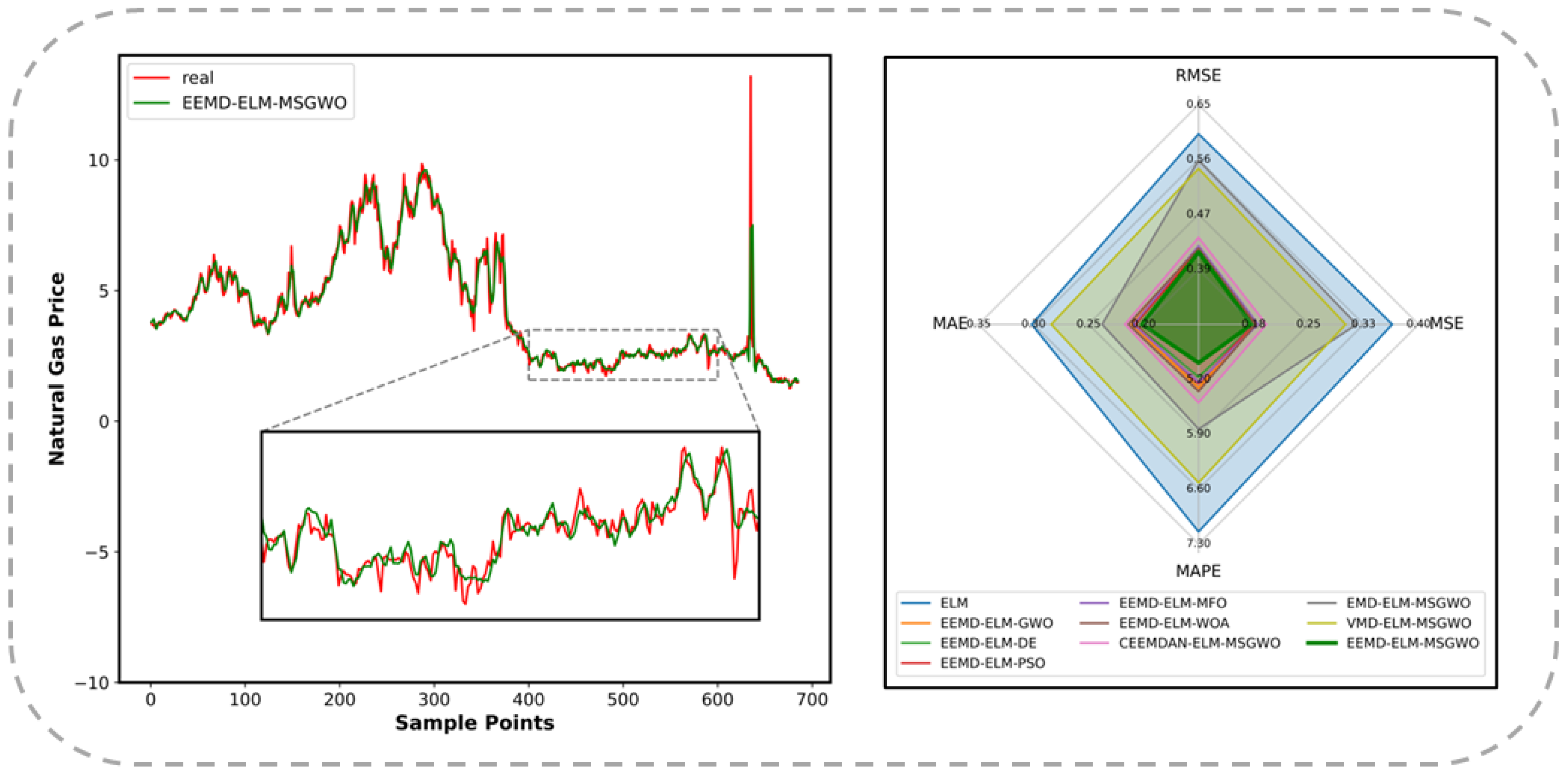
Upon attaining the optimal hidden layer matrices, the forecasting models became operational. The methodological phase transitions to the temporal partitioning of IMFs into calibration and validation subsets. The newly constructed forecasting models were trained using the training sets of IMFs corresponding to each set of hidden layer matrices optima and evaluated using the testing sets. To ensure statistical robustness, each configuration was autonomously executed in ten trials under identical environmental constraints. Subsequent analysis quantifies the metrics across multiple dimensions, as listed in

Table 6. Statistical table of point forecast results (Decomposition-ELM-Algorithm).

Model	MSE	RMSE	MAE	MAPE
ELM	0.3641	0.6034	0.3017	7.1425
EEMD-ELM-GWO	0.1761	0.4194	0.2107	5.3096
EEMD-ELM-DE	0.1750	0.4181	0.2073	5.1720
EEMD-ELM-PSO	0.1748	0.4178	0.2078	5.2566
EEMD-ELM-MFO	0.1812	0.4251	0.2092	5.2369
EEMD-ELM-WOA	0.1783	0.4214	0.2138	5.3537
CEEMDAN-ELM-MSGWO	0.1925	0.4383	0.2169	5.4972
EMD-ELM-MSGWO	0.3155	0.5615	0.2377	5.8349
VMD-ELM-MSGWO	0.3005	0.5481	0.2839	6.5182
EEMD-ELM-MSGWO	0.1723	0.4151	0.2016	4.9903

. The visualizations in Figure 10 illustrate the alignment fidelity of the EEMD-ELM-MSGWO framework with market observations.

Through rigorous interrogation of the quantitative evidence presented above, three principal findings emerged from the experiment.

First, through the implementation of EEMD-based signal decomposition, MSGWO exhibits superior efficacy in neural parameter optimization compared to conventional metaheuristics. Among the six competing architectures, the EEMD-ELM-MSGWO synthesis achieves minimal prognostic deviation, securing a dominant position across all evaluation criteria. These results indicate that the hidden layer matrices of the ELM that are most suitable for predicting the natural gas price can be effectively determined by the MSGWO. As an enhanced metaheuristic algorithm, the MSGWO innovatively integrates the GWO with three strategies. It utilizes mutation and crossover strategies to enhance population diversity, thereby broadening the scope of the global search. Meanwhile, the powerful local search ability of the GWO is retained. The inclusion of selection strategies allows the wolf pack to explore more promising directions, further improving the convergence speed and optimization capability of the MSGWO. The search characteristics of GWO and the three major strategies can be effectively utilized by MSGWO, enabling comprehensive traversal of hyperdimensional solution spaces and accelerated identification of the globally optimal gray wolf. In MSGWO, the search strategy of GWO and the mechanisms of mutation and crossover for generating new individuals are selected based on the difference between the incumbent optimal candidate and its ancestral best solution from prior iterations. This method effectively prevents the GWO or the mutation and crossover strategies from getting trapped in local optima. The MSGWO achieves balanced exploration-exploitation dynamics, facilitating the convergence of optimal neural parameters for the ELM.

Secondly, by using the EEMD to decompose the natural gas price and employing the MSGWO to establish minimum-error neural configurations, the resulting predictions are the closest to the observed values compared to alternative decomposition modalities. In the experimental simulations involving CEEMDAN-ELM-MSGWO, EMD-ELM-MSGWO, VMD-ELM-MSGWO, and EEMD-ELM-MSGWO, the EEMD-ELM-MSGWO model achieves minimal prognostic deviation. Compared with the original ELM model, the EEMD-ELM-MSGWO model exhibited a reduction of over 25% across all four statistical indicators. Furthermore, EEMD-ELM-MSGWO demonstrates enhanced robustness compared to competing decomposition-prediction hybrids, empirically validating EEMD’s methodological superiority in temporal decomposition fidelity for natural gas price forecasting. EEMD, developed on the EMD, has undergone multiple improvements and optimizations, making it more effective in capturing the characteristics and variations at different scales in natural gas price time series data. By adding white noise signals, the noise interference within the original signal can be suppressed using EEMD. This approach allows the EEMD to better extract the true components of the signal, thereby reducing the effects of noise and improving the decomposition accuracy. Moreover, the EEMD effectively reduces the occurrence of mode mixing, enhancing the clarity and interpretability of the decomposition results. Owing to its ability to better reflect the features and variations within the natural gas price series, the EEMD-ELM-MSGWO model surpasses other ELM-MSGWO models that incorporate different decomposition techniques, achieving the most accurate point-forecasting results.

5.6. Discussion

This section undertakes a deeper interrogation of experimental data to elucidate the multi-dimensional interdependencies among time series decomposition, hidden layer matrix optimization, and the accuracy of natural gas price prediction. Quantitative findings establish that the comprehensive model achieves lower prediction errors than the unimodal approaches, emphasizing only either decomposition or parametric refinement. The integrated model comprises three synergistic phases: (1) decomposition of the natural gas price through EEMD, (2) intelligent optimization of hidden layer matrices via MSGWO, and (3) prognostic execution through enhanced ELM.

Compared to ELM-MSGWO, EEMD-ELM-MSGWO exhibited marked prognostic enhancement, with MSE reduction surpassing 50%, RMSE decrease exceeding 30%, and the decrease in MAE and MAPE exceeding 10%. Similarly, the performance of EEMD-ELM-MSGWO compared with that of the EEMD-ELM model also shows significant progress. These statistical results substantiate the beneficial effects of first decomposing the signal in time-series forecasting and then optimizing neural parameters through the MSGWO algorithm on prediction accuracy. At the same time, these data validate the operational efficacy of the proposed EEMD-ELM-MSGWO.

The pre-decomposition of time series data before prediction and the post-prediction recombination of results play crucial roles in time series forecasting [46]. Signal decomposition techniques enable the enhanced detection of time-series data, thereby better capturing the overall direction of the time series. Concurrently, these techniques isolate cyclical constituents manifesting recurring oscillations, empowering models to precisely characterize periodic phenomena. Residual components encapsulate irreducible stochastic elements beyond deterministic trends and cycles, predominantly comprising of aleatoric noise. The characteristics and trends of each sub-series can be better captured by decomposing the time series into IMFs and residuals, thereby improving the prediction accuracy. As energy market quotations exhibit non-stationary characteristics, natural gas price trajectories are shaped by multi-factorial influences, including cyclical demand variations, regulatory interventions, and supply−demand dynamics. The accuracy of predictions can be improved to a large extent by processing natural gas price series using a decomposition method before feeding them into a predictor. This finding is consistent with previous studies [61,62,63], which also emphasized the benefits of combining decomposition techniques with machine learning or deep learning models. However, different signal decomposition techniques exhibit slight differences in their ability to decompose natural gas price series. In the comparative analysis, the EEMD established theoretical superiority for natural gas price series processing through its noise-assisted stabilization mechanism. By adding white noise signals to suppress noise interference in the original signals, the EEMD ensures algorithmic robustness against signal distortion, ultimately attaining optimal prognostic fidelity and computational consistency.

Moreover, the nonlinear dynamics and high volatility of natural gas prices present a dual challenge for optimization algorithms: they must effectively explore a complex, multimodal search space while avoiding premature convergence to the local optima. Accurate forecasting in this domain requires not only high predictive accuracy but also robust generalization across varying market conditions. In this regard, the proposed MSGWO algorithm outperformed conventional intelligent approaches, such as PSO, MFO, and WOA, owing to its enhanced spatial diversity preservation mechanism. This feature helps maintain a healthy exploration–exploitation balance, thereby improving the accuracy of the parameter optimization and enhancing the robustness of the forecasting model. Consequently, the MSGWO is better equipped to accommodate the inherent uncertainty and abrupt fluctuations characteristic of natural gas markets. The suggested MSGWO combines GWO with mutation, crossover, and selection strategies. It implements mutation and crossover strategies to maintain swarm heterogeneity, thereby expanding the search area. The selection strategy guides the population in more promising directions. The integration of these three strategies effectively compensates for GWO’s shortcomings in global search. Additionally, MSGWO uses a selection mechanism that compares the current optimal individual with the optimal individual of the previous generation to determine the search direction of the next generation. This mechanism effectively balances global and local searches, enabling the ELM model to converge to optimal neural configuration parameters that maximize prognostic fidelity. This is evident from the comparison between ELM-MSGWO and ELM-GWO, as well as between EEMD-ELM-MSGWO and EEMD-ELM-GWO. Among the decomposition methods, EEMD provides the most reasonable decomposition of the series, while MSGWO demonstrates the strongest global optimization capability. Therefore, by applying EEMD-driven decomposition and leveraging MSGWO’s robust global and local search abilities, the highest prediction accuracy model among all experimental groups can be achieved.

Additionally, the computational complexity of the EEMD-ELM-MSGWO model primarily arises from the EEMD decomposition, ELM training, and MSGWO optimization steps. To verify that the proposed model achieves high prediction accuracy with a reasonable computational cost, we compare its runtime and prediction performance metrics with those of other models. The results are shown in

Table 7. Comparison of prediction performance and computational time for the different models.

Model	MSE	MAE	Total Time (s)
LSTM	0.4687	0.3391	59.5468
CNN	2.0780	1.0395	48.2119
TCN	0.6146	0.5170	133.1150
Transformer	0.5164	0.4962	284.5282
EEMD-ELM-GWO	0.1761	0.2107	174.1935
EEMD-ELM-DE	0.1750	0.2073	279.0619
EEMD-ELM-MSGWO	0.1723	0.2016	155.8638

.

As shown in Table 7, the proposed EEMD-ELM-MSGWO model achieved the lowest prediction error among all the comparative models while maintaining a competitive computational efficiency. Given that accurate price forecasting is essential in energy trading, risk management, and policy formulation, the model demonstrates a favorable balance between prediction accuracy and computational cost, making it suitable for real-world applications. The EEMD decomposition can be efficiently accelerated using parallel computing techniques, thereby significantly reducing the runtime. Furthermore, the utilization of modern computing resources—such as GPU acceleration—can further alleviate the computational burden, enhancing the scalability and practical applicability of the model in large-scale data processing scenarios.

6. Probability Interval Forecasting

As shown in the graphical and numerical data presented in Figure 4 and Table 3, the temporal dataset utilized for probability interval prediction maintains temporal coherence with point-forecasting inputs. The methodology employs a training corpus of 6158 temporal observations, whereas the validation subset comprises 685 chronologically ordered entries.

The present investigation implements a dual-aspect experimental design to evaluate probability interval forecasting models through (1) EEMD-based temporal decomposition synergized with metaheuristic-driven neural parameter optimization for the PFELM model and (2) MSGWO-driven neural parameter optimization for the PFELM model after applying different decomposition techniques.

The experiments are conducted four times to systematically validate the forecasting capabilities of the PFELM model and the suggested probability interval forecasting framework at multiple confidence levels ($\alpha =0.025, 0.05, 0.075, \mathrm{a}\mathrm{n}\mathrm{d} 0.1$). All computational implementations maintain identical infrastructure specifications, with prognostic outputs undergoing analysis. The statistical data are tabulated in

Table 8. Statistical table of probability-interval forecast results.

CI	Model	PICP	PINAW	CWC
80%	EEMD-PFELM-GWO	0.65	1.25	27,991.96
	EEMD-PFELM-DE	0.65	1.15	28,994.68
	EEMD-PFELM-PSO	0.66	1.18	14,709.33
	EEMD-PFELM-MFO	0.68	1.13	7420.93
	EEMD-PFELM-WOA	0.64	0.98	37,039.12
	CEEMDAN-PFELM-MSGWO	0.63	1.05	56,483.09
	EMD-PFELM-MSGWO	0.67	1.13	9931.76
	VMD-PFELM-MSGWO	0.55	0.90	952,079.38
	EEMD-PFELM-MSGWO	0.70	1.09	3773.75
85%	EEMD-PFELM-GWO	0.74	1.54	776.04
	EEMD-PFELM-DE	0.76	1.42	355.63
	EEMD-PFELM-PSO	0.74	1.45	978.62
	EEMD-PFELM-MFO	0.78	1.39	163.93
	EEMD-PFELM-WOA	0.74	1.21	812.57
	CEEMDAN-PFELM-MSGWO	0.73	1.30	1039.77
	EMD-PFELM-MSGWO	0.76	1.39	414.92
	VMD-PFELM-MSGWO	0.65	1.11	24,850.76
	EEMD-PFELM-MSGWO	0.79	1.35	99.81
90%	EEMD-PFELM-GWO	0.83	1.91	38.30
	EEMD-PFELM-DE	0.85	1.76	15.73
	EEMD-PFELM-PSO	0.84	1.80	24.58
	EEMD-PFELM-MFO	0.87	1.72	8.13
	EEMD-PFELM-WOA	0.83	1.49	22.76
	CEEMDAN-PFELM-MSGWO	0.82	1.60	35.98
	EMD-PFELM-MSGWO	0.85	1.72	16.23
	VMD-PFELM-MSGWO	0.72	1.37	1976.45
	EEMD-PFELM-MSGWO	0.87	1.67	6.87
95%	EEMD-PFELM-GWO	0.92	2.45	3.50
	EEMD-PFELM-DE	0.93	2.26	2.98
	EEMD-PFELM-PSO	0.91	2.31	3.63
	EEMD-PFELM-MFO	0.94	2.21	2.61
	EEMD-PFELM-WOA	0.93	1.91	2.60
	CEEMDAN-PFELM-MSGWO	0.91	2.06	3.64
	EMD-PFELM-MSGWO	0.93	2.21	2.77
	VMD-PFELM-MSGWO	0.82	1.76	41.89
	EEMD-PFELM-MSGWO	0.94	2.14	2.50

, and Figure 11 demonstrates the EEMD-PFELM-EGWO uncertainty trajectories.

Through a systematic evaluation of the evidentiary matrix in Table 8, three axiomatic conclusions emerge:

(1)

Through EEMD-based temporal decomposition, the proposed MSGWO algorithm exhibits superior efficacy in resolving neural connection parameters for the PFELM model. Across the four confidence levels, the proposed EEMD-PFELM-MSGWO consistently ranks first. This indicates that the EEMD-PFELM-MSGWO can perform robust and precise probabilistic predictions under multi-scale uncertainty conditions, exhibiting superior performance to other models. Once again, MSGWO proves its efficacy in finding optimal parameters. MSGWO not only demonstrates excellent parameter optimization ability in deterministic forecasting but also effectively enables PFELM to broaden the coverage range of the probability forecasting interval while reducing its width, thereby improving the volatility regime adaptability of PFELM. Built upon the traditional GWO, MSGWO introduces a series of innovative mechanisms to enhance the performance of the wolf pack in global optimization problems. Regarding the search capability and convergence speed, the synergistic effect of these mechanisms enables the MSGWO to outperform other optimization algorithms, making it a powerful tool for addressing complex practical issues. The outstanding performance of MSGWO has not only been validated theoretically but also provides reliable and efficient solutions for various optimization problems encountered in practical applications.

(2)

Before optimizing the PFELM using MSGWO, employing the EEMD technique for the signal decomposition of the natural gas price series led to more accurate probability forecasting results. In the experiments of the EMD-PFELM-MSGWO, CEEMDAN-PFELM-MSGWO, VMD-PFELM-MSGWO, and EEMD-PFELM-MSGWO, the statistical indicators of the EEMD-PFELM-MSGWO outperform the other three models at all confidence levels. These findings demonstrate EEMD’s significant capacity to optimize probability forecasting models. This can be attributed to the noise-handling capability and multi-scale decomposition ability of EEMD. Compared to other decomposition methods, the results obtained from the EEMD decomposition are more comprehensive, providing richer information that serves as a better data foundation for subsequent analyses and modeling. Furthermore, the EEMD efficiently reduces mode-mixing phenomena, enhancing clarity and interpretability. This operational characteristic ensures decomposition stability by preventing inter-component interference, ultimately amplifying the temporal resolution and decomposition consistency.

7. Quantile Interval Forecasting

As shown in Figure 4 and Table 3, the quantile-based forecasting interval analysis maintains identical temporal data partitioning as employed in previous stages. The model training utilizes a dataset of 6158 observations, with the validation subset containing 685 entries for prognostic verification.

To provide additional confirmation of the operational efficacy of the suggested forecasting framework, this experimental stage compares the models at various quantile levels using distinct temporal decomposition methods and those combining different metaheuristic optimization algorithms. Through a cross-paradigm evaluation of various decomposition approaches and intelligent optimization algorithms, we can acquire knowledge of their potency in the optimization process, directing the choice of the most appropriate algorithm for specific tasks.

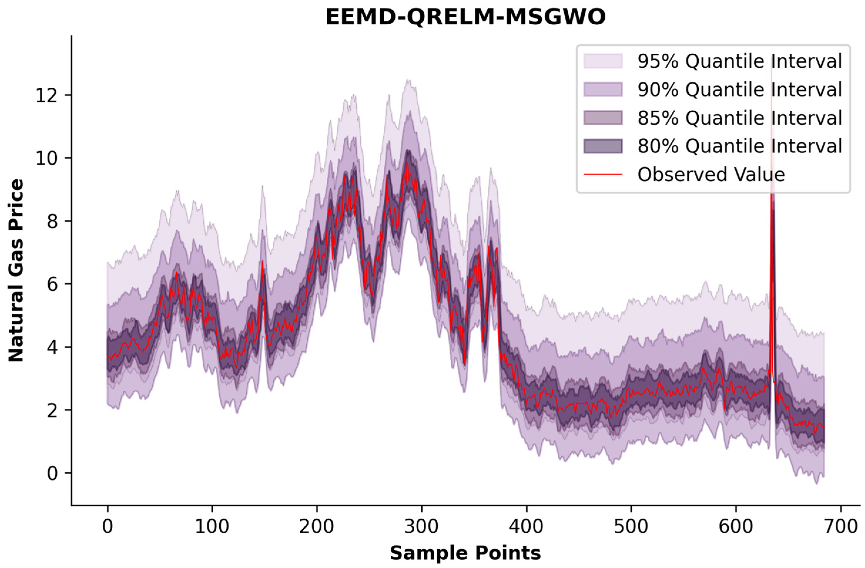
The experiments were performed in quadruple experimental iterations to assess the prognostic performance of the QRELM and ensure methodological replicability. Different quantile levels $\tau =0.025$, $\tau =0.05$, $\tau =0.075$, and $\tau =0.1$ correspond to confidence levels of 95%, 90%, 85%, and 80%, respectively, in quantile interval forecasting. All computational trials maintained identical infrastructure specifications and OS kernel parameters, followed by prognostic output post-processing and systematic evaluation of the forecasting results. The quantile forecasting performance metrics are tabulated in

Table 9. Statistical table of the quantile interval forecast results.

CI	Model	PICP	PINAW	CWC
80%	EEMD-QRELM-GWO	0.94	1.13	1.13
	EEMD-QRELM-DE	0.96	1.42	1.42
	EEMD-QRELM-PSO	0.94	1.03	1.03
	EEMD-QRELM-MFO	0.96	1.47	1.47
	EEMD-QRELM-WOA	0.96	1.50	1.50
	CEEMDAN-QRELM-MSGWO	0.97	1.44	1.44
	EMD-QRELM-MSGWO	0.99	2.28	2.28
	VMD-QRELM-MSGWO	0.86	1.15	1.15
	EEMD-QRELM-MSGWO	0.93	0.92	0.92
85%	EEMD-QRELM-GWO	0.98	2.28	2.28
	EEMD-QRELM-DE	0.98	1.78	1.78
	EEMD-QRELM-PSO	0.98	1.83	1.83
	EEMD-QRELM-MFO	0.99	1.81	1.81
	EEMD-QRELM-WOA	0.97	1.50	1.50
	CEEMDAN-QRELM-MSGWO	0.98	1.64	1.64
	EMD-QRELM-MSGWO	0.98	2.12	2.12
	VMD-QRELM-MSGWO	0.99	2.96	2.96
	EEMD-QRELM-MSGWO	0.97	1.40	1.40
90%	EEMD-QRELM-GWO	1.00	4.17	4.17
	EEMD-QRELM-DE	0.99	3.69	3.69
	EEMD-QRELM-PSO	1.00	3.41	3.41
	EEMD-QRELM-MFO	1.00	4.52	4.52
	EEMD-QRELM-WOA	1.00	3.56	3.56
	CEEMDAN-QRELM-MSGWO	0.98	3.72	3.72
	EMD-QRELM-MSGWO	0.99	3.61	3.61
	VMD-QRELM-MSGWO	1.00	5.46	5.46
	EEMD-QRELM-MSGWO	1.00	3.25	3.25
95%	EEMD-QRELM-GWO	1.00	7.53	7.53
	EEMD-QRELM-DE	1.00	7.78	7.78
	EEMD-QRELM-PSO	1.00	8.81	8.81
	EEMD-QRELM-MFO	1.00	7.01	7.01
	EEMD-QRELM-WOA	1.00	7.90	7.90
	CEEMDAN-QRELM-MSGWO	1.00	7.53	7.53
	EMD-QRELM-MSGWO	1.00	10.75	10.75
	VMD-QRELM-MSGWO	1.00	9.02	9.02
	EEMD-QRELM-MSGWO	0.99	3.81	3.81

, and Figure 12 visualizes the EEMD-QRELM-MSGWO synthesis’s trajectory alignment with market dynamics.

As evidenced by the comparative analysis in Table 9, the proposed MSGWO optimization framework exhibits superior efficacy in identifying neural configuration parameters that minimize the quantile prediction error for QRELM architectures. Through prognostic simulation experiments comparing five distinct probabilistic regression frameworks—designated as GWO-based, DE-driven, PSO-optimized, MFO-enhanced, and MSGWO-integrated EEMD-QRELM variants—the proposed MSGWO consistently ranks first at all quantile levels, showcasing the strongest overall interval prediction capability. This indicates that the EEMD-QRELM-MSGWO model can consistently and accurately perform quantile-interval forecasting tasks and exhibits excellent performance across different levels of uncertainty. These empirical results substantiate the framework’s capacity for precision-calibrated distribution estimation under market conditions, providing actionable intelligence for risk quantification and volatility hedging strategies in the natural gas market.

Compared with the other three signal decomposition techniques, EEMD significantly enhanced the accuracy of the QRELM-MSGWO quantile interval forecasting model. By inheriting the advantages of EMD and addressing its shortcomings, EEMD can handle nonlinear and non-stationary signals more effectively, thereby improving the precision of signal decomposition. Furthermore, the EEMD employs a method of adding white noise, which can dynamically adjust the noise level, thereby effectively suppressing endpoint distortion while maintaining intrinsic oscillatory characteristics. EEMD also demonstrably reduces the occurrence of mode mixing, preventing mutual interference among the signal components and thus enhancing the precision and reliability of the decomposition. The accurate subsequences generated by the EEMD contain more scale information, which helps the QRELM-MSGWO model better grasp the features of the natural gas price series, leading to more precise quantile interval forecasting results.

The effectiveness of MSGWO in optimizing parameters was reaffirmed. The MSGWO excels in parameter optimization for point and probability interval forecasting and significantly reduces the quantile loss for the QRELM model as well. By improving the coverage rate of the quantile forecasting interval while reducing the average width of the forecasting interval, MSGWO enables the QRELM to achieve a quantile-interval-forecasting model that balances precision and robustness. Compared to the original GWO algorithm, MSGWO incorporates a series of innovations that enhance the algorithm’s performance in solving optimal parameter determination problems. The MSGWO leverages GWO’s powerful local search mechanism while using mutation and crossover strategies to increase population diversity, thereby strengthening the exploration of unknown regions. The selection mechanism ensures that the population searches in the correct direction. The fusion of these mechanisms makes the MSGWO’s exploration of the solution space comprehensive and effectively avoids local optima. Consequently, MSGWO stands out among the numerous intelligent algorithms.

8. Conclusions

This paper proposes a composite framework for sequential data forecasting using signal decomposition methods and metaheuristic optimization. The framework utilizes the EEMD to disintegrate the natural gas market quotations into IMFs and employs the proposed MSGWO algorithm to improve the hidden layer weight and bias matrices of the ELM. The enhanced ELM is then trained with the training data and executes prognostic verification trials on the test sample. This established an effective prediction system. The GWO exhibits notable efficacy in neighborhood exploration. The incorporation of mutation and crossover strategies enhances the solution space diversity, thereby boosting the cross-domain search potential. In addition, the algorithm employs a selection strategy to ensure that the population advances in the correct search direction. Through such multi-mechanism fusion, MSGWO achieves balanced exploitation-exploration dynamics, enabling efficient traversal across high-dimensional parameter landscapes and precise identification of optimal neural configuration parameters, ultimately producing superior prognostic performance in energy market forecasting applications.

Forecasting experiments on natural gas price series are divided into three phases: point forecasting, probability interval forecasting, and quantile interval forecasting. In point forecasting, the proposed EEMD-ELM-MSGWO model achieves the smallest prediction error in several evaluation indexes and realizes the most accurate prediction effect. With the acceleration of the global energy transition and increasing involvement of financial markets, natural gas price uncertainty is influenced by a range of market factors, including supply and demand dynamics, pricing of alternative energy sources, and pronounced seasonal sensitivity [64]. Moreover, climate policies in various countries have dampened investments in fossil energy [65], while reductions or disruptions in gas supply caused by geopolitical events, such as the Russia–Ukraine conflict [66], and demand shocks triggered by emergencies, such as the COVID-19 pandemic, have further exacerbated the volatility in overall gas consumption [67]. Although probabilistic forecasting and quartile interval prediction can effectively capture and quantify such uncertainty, developing appropriate forecasting models is essential to support their implementation. In probability and quantile interval forecasting, the proposed EEMD-PFELM-MSGWO model and EEMD-QRELM-MSGWO model achieve the minimum level of CWC, indicating that the EEMD-PFELM-MSGWO and EEMD-QRELM-MSGWO models in interval coverage forecasting and forecasting under different quantiles can capture the uncertainty in the natural gas price series well. Three experiments confirmed the efficacy of the proposed EEMD-ELM-MSGWO forecasting composite framework.

Point forecasting of natural gas price series helps in understanding and forecasting future market price trends and provides valuable references for decision-makers. Probability interval forecasting quantifies uncertainty and offers decision-makers probability information regarding various potential outcomes. Quantile interval forecasting further delineates the range of price changes, aiding decision-makers in comprehensively assessing the risks and formulating appropriate strategies. These methods provide natural gas market participants with more comprehensive and accurate future price trend information, enabling the formulation of well-informed commercial strategies and regulatory frameworks.

However, it is important to acknowledge the limitations of this study that should be addressed in future research. First, the current model relies solely on historical price data and does not incorporate exogenous variables such as policy changes, exchange rates, or geopolitical events, which may affect the model’s predictive performance during periods of sudden market fluctuations. Future work will aim to examine the drivers of natural gas prices from multiple perspectives and integrate an online learning mechanism to enable the model to dynamically adapt to market uncertainties. Second, the model validation is currently limited to a single natural gas market. Given the diversity in pricing mechanisms across global markets, future research should consider using different data sources to evaluate the model’s applicability and robustness in other countries and regions.