Spatiotemporal Evolution of Ecosystem Service Value and Its Tradeoffs and Synergies in the Liaoning Coastal Economic Belt

Abstract

As ecologically sensitive interfaces shaped by the interplay of land and sea, coastal zones demand close attention. Uncovering the spatiotemporal evolution of ecosystem service value (ESV) and the intricate interrelations among ecosystem service (ES) functions is imperative for the informed governance of human–land interactions and for fostering sustainable regional development. This study analyzes the spatiotemporal evolution of ESV based on the modified equivalent factor table, combining the Geo-information Tupu, Markov transfer model, and standard deviation ellipse. Additionally, we introduce an ecosystem service tradeoff degree (ESTD) to assess the tradeoffs and synergies among various ESs, and we utilize GeoDetector to elucidate the driving forces behind the spatial disparities in ESV. Our findings reveal that (1) Although the land use composite index in the Liaoning coastal economic belt (LCEB) increased, the pace of land use transformation demonstrated a trend toward stabilization over the study duration. (2) Between 2000 to2020, ESV initially declined but subsequently experienced an upward rebound, resulting in a net gain of approximately 48 billion yuan. Spatial analysis indicated continuous enlargement of the standard deviation ellipse, with its centroid consistently located within Yingkou City and a gradual directional shift toward the southwest. (3) The dominant relationship among ESs showed synergy, with notable tradeoffs between hydrological regulation and other services. (4) Topography and climate factors were the primary drivers of spatial heterogeneity of ESV in the LCEB. The research provides spatial decision support for optimizing the ecological security pattern of the coastal zone.

1. Introduction

Ecosystem services (ESs) serve as a fundamental link between natural capital and human well-being [1]. Encompassing provisioning services (e.g., food production), regulating services (e.g., climate regulation, forest carbon sinks), supporting services (e.g., soil formation, habitat provision), and cultural services (e.g., recreation, cultural heritage), they now stand at the forefront of the global sustainable development agenda [2]. However, the Global Environment Outlook 2019 reports that land degradation, water scarcity, and sharp declines in biodiversity have led to functional degradation or continued deterioration in over 40% of the world’s ecosystems [3,4]. Consequently, reconciling the imperative of ecosystem protection with the rational utilization of their services has emerged as a pressing and globally shared concern among scholars.

In recent years, the spatiotemporal evolution of ecosystem service value (ESV) and its underlying drivers has risen to the forefront of ecological and geographical inquiry. At the methodological level of ESV assessment, researchers have made significant advances. The equivalence factor method, advanced by Xie Gaodi’s team, has notably enhanced multi-scale evaluation accuracy through localized parameter adjustments and has seen broad empirical application [5,6]. Moreover, the Integrated Valuation of Ecosystem Services and Tradeoffs (InVEST) model, devised by the Natural Capital Project in the United States, leverages multi-scenario simulations to deliver adaptive, evidence-based decision support for spatial planning initiatives [7]. Contemporary ESV research predominantly focuses on three domains: (1) mapping the spatiotemporal distribution and evolutionary trends of ESV; (2) examining tradeoffs and synergies among ESs; and (3) simulating potential future trajectories under varying scenarios. Despite these advancements in thematic depth, several methodological limitations persist: (1) spatiotemporal analyses remain limited in scope—conventional hotspot mapping and spatial autocorrelation techniques fall short in capturing ESV grade transitions, thus constraining deeper insights into landscape dynamics [8,9]; (2) most tradeoffs/synergies analyses rely on statistical assumptions, while linear models tend to undervalue the nonlinear interactions inherent in complex geographic systems [10]; and (3) the majority of studies focus exclusively on either terrestrial or marine systems, overlooking the coupled dynamics of land–sea transitional zones and thus failing to fully elucidate the spatiotemporal behavior of ESV [11,12]. In contrast to traditional methods, Geo-information Tupu approaches offer a systematic lens to unravel the multi-dimensional transformations of geographic features [13] and the Markov model enables precise depictions of state transitions in geographic phenomena from T₀ to T₁ via transition matrices. Meanwhile, the standard deviation ellipse model visualizes the spatial differentiation and dynamic trajectory of ESV via centroid displacement and directional spread [14]. Building on these insights, we propose an integrative framework coupling Geo-information Tupu with Markov transition models, offering a fresh paradigm for illuminating the spatiotemporal evolution of ESV.

The interplay of tradeoffs and synergies among ESs constitutes a pivotal scientific challenge in advancing optimal resource management [15]. A tradeoff describes the inverse relationship whereby the enhancement of one service diminishes another, whereas a synergy implies concurrent improvements or declines across multiple services [16]. In recent years, these dynamics have garnered considerable attention in ecological research, becoming a key focus for scholars worldwide. It is now widely acknowledged that tradeoffs and synergies are pervasive features of ES interactions [17,18]. From a spatiotemporal standpoint, tradeoffs can be classified into temporal, spatial, and reversible categories [19,20]. Methodologically, researchers have employed statistical analysis, spatial mapping, and scenario modeling—drawing upon tools such as correlation and regression analyses, the InVEST model, the CA-Markov model, and the CLUE-S model—to explore tradeoffs/synergies relationships, spatial patterns, and underlying mechanisms [21,22,23,24]. Yet, conventional approaches often overlook the nonlinear nature of service interactions and fall short in capturing the dynamic modulation effects of multi-scale drivers [25]. To address this gap, the present study introduces the ecosystem services tradeoff degree (ESTD) model, which precisely identifies critical tipping points in ESV interactions and offers a novel framework for coordinated, multi-objective management of coastal regions.

A number of scholars have undertaken preliminary studies on ESs within the Liaoning Coastal Economic Belt (LCEB). Yet, these investigations are often limited by their short temporal scope, provide insufficient exploration of the interdependencies among distinct ES functions, and fall short of offering a thorough analysis of the spatiotemporal evolution of ESV and its underlying drivers [26]. Strategically situated at the nexus of the Northeast Asian Economic Belt and the Bohai Rim Economic Zone, the LCEB functions as a critical gateway for regional openness and integration, underscoring its geopolitical and economic importance [27]. In addition, the LCEB diverse coastal and marine habitats deliver a suite of essential Ess, including habitat provision, blue carbon storage, coastal flood and storm attenuation, and the regulation of sediment dynamics and shoreline stability. Decades of intensive exploitation of coastal and marine resources have precipitated a series of critical ecological challenges, including excessive land reclamation, marine pollution, and drastic biodiversity loss. These environmental stressors compromise both the long-term sustainability of regional economic growth and the structural integrity of coastal ecosystems. As a densely populated and economically active zone—that simultaneously serves as a critical frontier for ecological stewardship and biodiversity conservation—the LCEB demands urgent, science-based strategies for sustainable ecosystem governance and restoration.

Against this backdrop, the objectives of this study include (1) to construct a Geo-information Tupu using the Markov transition model and standard deviation ellipse model to investigate the spatiotemporal evolution characteristics of ESV; (2) to apply the ESTD model for assessing tradeoffs and synergies among various ES functions; and (3) to utilize the geographical detector to examine how various potential driving forces contribute to the spatial variation of ESV, thereby providing a reference for ecological waste management and sustainable development in the LCEB.

2. Study Area and Data Sources

2.1. Study Area

As the northernmost coastal province in China, Liaoning Province enjoys a temperate climate with distinct seasons and moderate annual precipitation. The coastline stretches from the mouth of the Yalu River in the east and connects with Laolongtou of the Shanhai Pass in the west, totaling 2737.6 km, including 2110 km of mainland coastline and 627.6 km of island coastline. This study selects the LCEB as the research area, defining the boundary based on the “Millennium Ecosystem Assessment” (2005) and the actual conditions of the study area. The land area is delineated by the administrative divisions of six coastal cities in Liaoning (Dalian City, Dandong City, Jinzhou City, Yingkou City, Panjin City, and Huludao City), while the marine boundary is defined by the first 15 m isobath from the coastline [28]. The study area is located in China’s core of the Northeast Asia Economic Circle, boasting significant strategic and economic value. It is also one of China’s important industrial bases, rich in mineral resources and advanced manufacturing, playing a crucial role in the economic development of Northeast China. The scope of the research area is shown in Figure 1.

Following years of development, the traditional economic development model relying solely on land resource increment in the LCEB has become unsustainable, facing dual pressures of exploring new economic growth points and ecological protection in coastal areas. Driven by rapid urban expansion and rising population densities, coastal cities in Liaoning are placing substantial demands on natural resources. This intensification imposes mounting stress on ESs, undermining the long-term viability of the regional economy. Consequently, there is an urgent imperative to transition toward sustainable, low-carbon development pathways to revitalize and sustain competitive advantages [29]. In this context, the LCEB serves as a representative case for analyzing the spatiotemporal dynamics of ESV.

2.2. Data Sources

Land use data for 2000, 2010, and 2020 were obtained from the Resource and Environment Science Data Center of the Chinese Academy of Sciences (https://www.resdc.cn/, accessed on 15 April 2024) with a spatial resolution of 30 m. Using ArcGIS 10.2 software, the secondary types of land use data were reclassified into eight categories: farmland, forest land, grassland, inland freshwater, saltwater wetland, shallow waters, construction land, and unused land. Following Chuai et al., we used the economic value of the main food crops (corn, rice, and soybean) based on the historical average arable land area in the study area as the calculation basis [30]. The yield and planting area data were collected from the Liaoning Statistical Yearbook, Bulletins, and Statistical Yearbooks of the six coastal cities in Liaoning Province. At the same time, grain prices were selected based on the average market price in Liaoning Province in 2020 (https://lcj.ln.gov.cn/, accessed on 22 April 2024).

To thoroughly explore the characteristics and underlying drivers of changes in ESV within the study region, this study ultimately selected two major categories of nine indicators for the spatial heterogeneity analysis of ESV: (1) The natural environmental variables included elevation, slope, average annual precipitation, average annual temperature, average annual wind speed, and normalized vegetation index NDVI. Digital Elevation Model (DEM) data sourced from the Geospatial Data Cloud (https://www.gscloud.cn/, accessed on 6 April 2024); the slope was extracted from DEM data; Climatic parameters—average annual precipitation (PRE), average annual temperature (TEM), and average annual wind speed (WIN)— came from the Resource and Environment Science Data Center of the Chinese Academy of Sciences. NDVI came from the National Ecological Science Data Center (http://www.nesdc.org.cn/, accessed on 26April 2024). (2) Socio-economic variables included GDP, population density (POP), and land use. GDP and land use data came from the same source; population density data (POP) were obtained from the WorldPop website (https://hub.worldpop.org/, accessed on 30 April 2024). To prepare the variables for analysis, each factor was discretized using the natural breaks classification method in ArcGIS 10.2.

3. Research Methods

3.1. Land Use Dynamic Changes

3.1.1. Land Use Dynamic Index

(1)

Single land use dynamics

The land use dynamic degree primarily reflects the regional differences in the intensity and rate of land use change [31]. The single land use dynamic reflects the annual rate of change for that land use category [32]. The related formulas are as follows:

$$K={\displaystyle \frac{U_{i2}-U_{i1}}{U_{i1}}}\times {\displaystyle \frac{1}{t_2-t_1}}\times 100\%$$

(1)

In Formula (1), $K$ represents the single dynamic degree of a certain land use type; $U_{i1}$ and $U_{i2}$ represent the area of the $i$-th land type at time periods $t_1$ and $t_2$, respectively; $t_1$ and $t_2$ represent the research time period.

(2)

Comprehensive land use dynamics

The comprehensive land use dynamic can be used for research on regional differences in land use dynamics [33]. The related formulas are as follows:

$$S={\displaystyle \frac{{\sum }_{i=1}^n∆U_{i-j}}{2{\sum }_{i=1}^n∆U_{i{t}_1}}}\times {\displaystyle \frac{1}{T}}\times 100\%$$

(2)

In Formula (2), $S$ is the comprehensive land use dynamic index; $∆U_{i-j}$ is the transfer area from $i$-th land use type to the non $i$-th in the time period of $T$; $U_{{it}_1}$ is the area of the $i$-th land use type in the period of $T$; $T$ is the research duration.

3.1.2. Land Use Composite Index

The land use composite index captures both the intensity and scope of land utilization within a region, serving as an indicator of the degree to which land resources are exploited and managed by human activities. Based on the research by Zhuang Dafang combined with the specific regional conditions, index values are assigned to different land use types on a grade basis to quantify the degree of land use intensity in the region [34]. The related formulas are as follows:

$$L=100\times {\sum }_{i=1}^n(A_i\times C_i)$$

(3)

where $L$ is the land use composite index; $A_i$ represents the grading index assigned to the $i$-th land use category; $C_i$ denotes the proportional area occupied by land category $i$; $n$ is grading index of the land use type. The degree of land utilization increases as $L$ value increases. Among them, the classification index is 1 for unused land and wetlands, 2 for forests, grasslands, and water bodies, 3 for cultivated land, and 4 for artificial surfaces.

3.2. Estimation of ESV

Currently, the equivalent value coefficient method remains the most widely adopted approach for quantifying ESV [6,35]. Costanza used the equivalent factor method to estimate ESV in 1997 [35], and Xie Gaodi made amendments to the equivalent factor method based on China’s actual conditions and proposed the China Ecosystem Service Value Coefficient Table, which has been widely applied in China [6].

Based on previous research findings, the natural grain yield is g, typically estimated as 1/7 of the actual grain yield. In this study, the economic value of natural grain production is calculated based on the average cultivated land area in the study region across the observation period, serving as the foundational metric for valuation. According to the grain production, planting area, and grain prices of the main grain crops in the LCEB from 2000 to 2020, a unit factor value is calculated, with a value of 2100.25 yuan/ha. Finally, the value tables of the ES per unit area of different land use types are obtained (

Table 1. ESV per unit area of land use/cover types (yuan/ha).

Primary Classification	Secondary Classification	Farmland	Forest	Grassland	Inland Freshwater	Saltwater Wetland	Shallow Water	Unused Land
Provisioning services	Food supply	2320.77	530.31	490.06	840.10	1071.13	28,877.33	105.01
	Raw material supply	514.56	1218.14	721.08	241.53	1050.12	479.28	31.50
Regulating services	Air quality regulation	1869.22	4006.22	2534.30	808.59	3990.47	3957.91	136.52
	Climate regulation	976.61	11,987.15	6699.79	2404.78	7560.89	5255.24	105.01
	Waste treatment	283.53	3512.66	2212.26	5828.18	7560.89	0.00	430.55
	Regulation of water flows	3139.87	7844.42	4907.58	107,364.58	50,888.96	711.35	252.03
Supporting services	Maintenance of soil	1092.13	4877.82	3087.36	976.61	4851.57	0.00	157.52
	Fertility habitat services	357.04	4442.02	2807.33	2677.81	16,528.94	19,206.75	147.02
Cultural services	Cultural and amenity services	157.52	1947.98	1239.15	1984.73	9934.16	17,955.21	63.01
Total		10,711.26	40,366.73	24,698.89	123,126.93	103,437.12	76,443.08	1428.17

). The related formulas are as follows:

$$V_a={\displaystyle \frac{1}{7}}{\sum }_{r=1}^R{\displaystyle \frac{s_r{y}_r{p}_r}{S}}$$

(4)

In Formula (4), $V_a$ denotes the per unit area value of food production services provided by the farmland ecosystem (yuan/ha); $R$ represents the total number of main grain crop categories; $S_r$ refers to the sown area of the $n$ food crop (ha); $y_r$ represents the yield of $r$ food crops (kg/ha); $p_r$ represents the average market price of $r$ types of food crops (yuan/kg); $S$ signifies the aggregate sown area of principal food crops (ha).

By statistically calculating the total area of different land types, combined with Table 1, it is feasible to obtain the different ESV quantities. Finally, the ESV of the study area is obtained. The related formulas are as follows:

$$ESV={\sum }_{i=1}^n{A}_i\times {VC}_i$$

(5)

$${VC}_i={\sum }_{j=1}^k{e}_{ij}\times V_a$$

(6)

In Formula (5) and Formula (6), $ESV$ represents the total ESV; $A_i$ denotes the area corresponding to the $i$-th land use type; ${VC}_i$ is the equivalent ESV per hectare for that land type (Yuan/ha); $e_{ij}$ refers to the equivalent value of the $j$-th ES provided by the $i$-th land use type; $k$ is the total number of ES types.

3.3. Construction of the Geo-Information Tupu

(1)

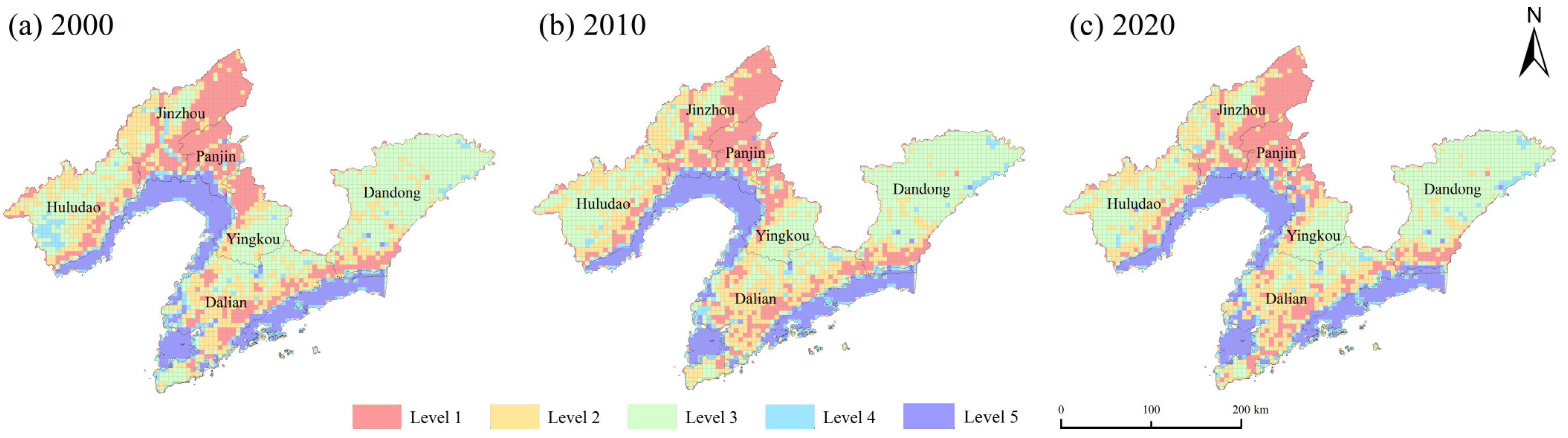
ESV’s spatiotemporal evolution Tupu. ArcMap 10.2 software is employed to create a 5 km × 5 km regular grid covering the study area, and the ESV of each grid is calculated [8,36]. According to relevant studies [37,38], the natural breakpoint grading approach is used to set the ESV classification criterion as follows: Level 1 (0, 1831.24 ten thousand yuan), Level 2 (1831.25, 3364.69 ten thousand yuan), Level 3 (3364.70, 5125.87 ten thousand yuan), Level 4 (5125.88, 7552.16 ten thousand yuan), and Level 5 (7552.17, 14,716.19 ten thousand yuan). Thus, we obtained the ESV’s spatial distribution maps in the LCEB.

(2)

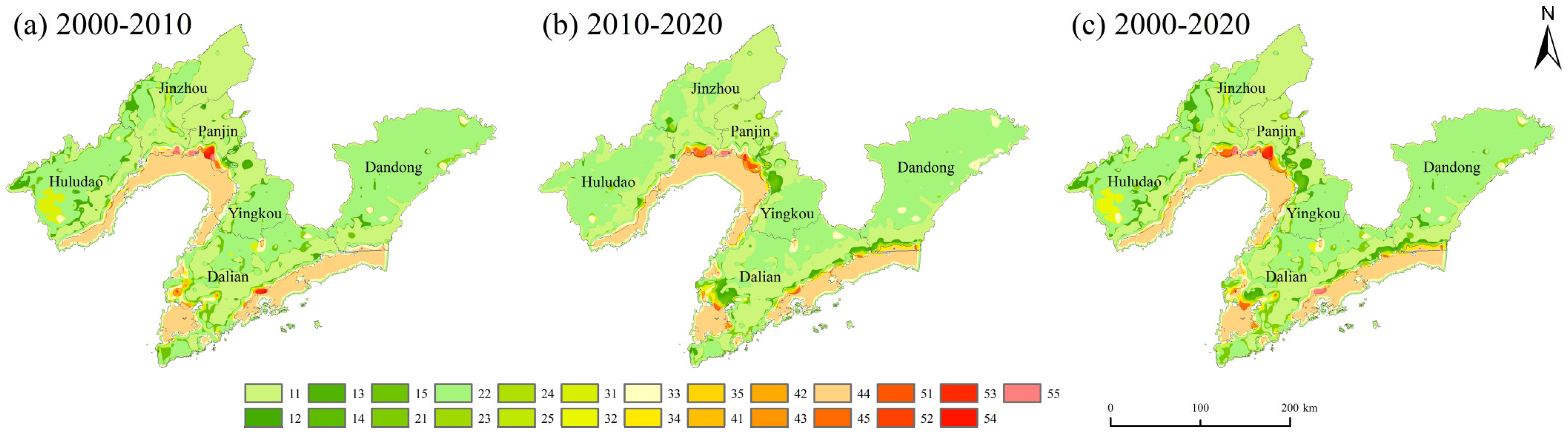
Transfer of ESV Tupu. The Markov transition model is a statistical framework grounded in probability theory, designed to capture the dynamics of system states transitioning from time T₀ to T₁. It operates under the assumption that the state at T₁ depends solely on the conditions at T₀, without influence from earlier periods [39]. In this study, the model is utilized to generate a transition matrix for the ESV, where each matrix element represents the area transferred between ESV levels. This approach facilitates a more detailed understanding of the spatial and temporal evolution of ESVs and provides a quantitative depiction of transitions among different ESV levels. The related formulas are as follows:

$$A_{ij}=\left[\begin{array}{ccc}\begin{array}{c}\begin{array}{cc}{A}_{11}& A_{12}\end{array}\\ \begin{array}{cc}{A}_{21}& A_{22}\end{array}\end{array}& \begin{array}{c}\dots \\ \dots \end{array}& \begin{array}{c}{A}_{1n}\\ A_{2n}\end{array}\\ \begin{array}{cc}⋮& ⋮\end{array}& ⋮& ⋮\\ \begin{array}{cc}{A}_{n1}& A_{n1}\end{array}& \dots & A_{nn}\end{array}\right]$$

(7)

In Formula (7), $A_{ij}$ represents the transfer probability of the ESV changing from level $i$ to level $j$, indicating either the quantity of area converted or the proportional relationship between levels. This probability satisfies the conditions 0 < $A_{ij}$ < 1 and ${\sum }_j^n{A}_{ij}$ = 1, meaning that the sum of each row’s elements equals one.

(3)

The rise-and-fall Tupu of the ESV is derived from the ESV transfer Tupu. Areas where the ESV level at time $T_1\mathrm{e}\mathrm{x}\mathrm{c}\mathrm{e}\mathrm{e}\mathrm{d}\mathrm{s}\mathrm{t}\mathrm{h}\mathrm{a}\mathrm{t}\mathrm{a}\mathrm{t}{ T}_0$ are defined as rising Tupu units, whereas those where the ESV level at ${ T}_1$ is lower than at ${ T}_0$ are identified as falling Tupus.

3.4. Standard Deviation Ellipse

The standard deviation ellipse is employed to characterize the orientation and spatial distribution of a set of data points [40,41]. To reflect the characteristics of the spatial distribution of the ESV from multiple perspectives, the standard deviation ellipse is employed to quantitatively analyze the regional gravity center position and spatial expansion direction of the ESV in the study area. Its elements consist of the azimuth, center, major axis, and minor axis. The related formulas are as follows:

$${\overline{X}}_w={\displaystyle \frac{{\sum }_{i=1}^n{w}_i{x}_i}{{\sum }_{i=1}^n{w}_i}}, {\overline{Y}}_w={\displaystyle \frac{{\sum }_{i=1}^n{w}_i{y}_i}{{\sum }_{i=1}^n{w}_i}}$$

(8)

$$\theta ={\displaystyle \frac{\arctan \left[\left({\sum }_{i=1}^n{x_i}^{\prime 2}-{\sum }_{i=1}^n{y_i}^{\prime 2}\right)+\sqrt{\left({\sum }_{i=1}^n{x_i}^{\prime 2}-{\sum }_{i=1}^n{y_i}^{\prime 2}\right)+4\left({\sum }_{i=1}^n{x_i}^{’2}{y_i}^{\prime 2}\right)}\right]}{2x{\sum }_{i=1}^n{x_i}^{\prime }{y_i}^{\prime }}}$$

(9)

$${\delta }_x=\sqrt{{\displaystyle \frac{{\sum }_{i=1}^n{\left({x_i}^{\prime }\cos \theta -{y_i}^{\prime }\sin \theta \right)}^2}{n}}}, {\delta }_y=\sqrt{{\displaystyle \frac{{\sum }_{i=1}^n{\left({x_i}^{\prime }\sin \theta -{y_i}^{\prime }\cos \theta \right)}^2}{n}}}$$

(10)

where ($\overline{X_w}$, $\overline{Y_w}$) signifies the weighted mean center; ($X_i$, $Y_i$) denote the coordinates of the county’s geometric centroid; $W_i$ represents the weight factor; $\theta$ corresponds to the azimuth angle of the ellipse; ${x_i}^{\prime }$ and ${y_i}^{\prime }$ represent the deviations of coordinates from the county centroid to the weighted mean center along the respective axes; ${\delta }_x$ and ${\delta }_y$ are the standard deviations along the $x$ and $y$ directions, respectively.

3.5. Ecosystem Service Tradeoff Degree (ESTD) Index

The ESTD is derived from linear regression analysis and captures both the direction and magnitude of interactions among various ESs [42,43]. Its primary aim is to provide an integrated assessment of how changes in ESs interrelate within the study area. A positive ESTD value signifies a synergistic relationship between the two ESs, whereas a negative value denotes a tradeoff. The magnitude of the absolute value represents the intensity of the synergy or tradeoff. The related formulas are as follows:

$${ESCI}_i={\displaystyle \frac{{ES}_{ia}-{ES}_{ib}}{{ES}_{ib}}}$$

(11)

$${ESTD}_{ij}={\displaystyle \frac{\frac{{ESCI}_i}{{ESCI}_j}+\frac{{ESCI}_j}{{ESCI}_i}}{2}}$$

(12)

where ${ESCI}_i$ denotes the change index of the $i$-th ES; ${ES}_{ia}$ represents the value of the $i$-th ES in $a$-th time (final state); ${ES}_{ib}$ corresponds to the value of the $i$-th ES in $b$-th time (initial state); ${ESTD}_{ij}$ quantifies the tradeoffs/synergies degree between the $i$-th and the $j$-th ESs.

3.6. Geographical Detector

The geographical detector detects spatial heterogeneity and reveals the driving force of various factors for the dependent variable, including four detectors [21,44]. This research applies factor and interaction detection techniques to discern and quantify the key drivers influencing the spatiotemporal evolution of the ESV within the study region [45]. The related formulas are as follows:

$$q=1-{\displaystyle \frac{\sum _{h=1}^L{n}_h{\sigma }_h^2}{n{\sigma }^2}}$$

(13)

where $q$ represents the explanatory power for changes in the ESV, ranging between 0 and 1. The magnitude of $q$ reflects the intensity of the factors’ influence on the evolution of the ESV—the larger the value, the more pronounced the effect; $n_h$ denotes the counts of county units within category $h$, and $n$ denotes the total counts of county units, respectively; ${\sigma }_h^2$ and ${\sigma }^2$ signify the variance of the ESV within category $h$ and across the entire set of county units, respectively.

4. Results

4.1. Land Use Change Characteristics

The land structure in the LCEB is diverse, with farmland and forest land being the primary land use types, accounting for over 32% and 33% of the total area, respectively (

Table 2. Changes in the area of different land use types in the LCEB from 2000 to 2020.

Land Use Type	Year	Farmland	Forest	Grassland	Inland Freshwater	Saltwater Wetland	Shallow Water	Construction Land	Unused Land
Area (km2)	2000	24,059.44	23,838.51	1656.20	1933.10	281.66	12,914.67	4071.27	1061.12
	2010	23,232.16	23,848.24	1090.90	2090.75	425.98	12,529.30	5673.83	1099.46
	2020	22,787.49	23,716.01	1052.00	3113.82	135.62	12,277.52	5918.17	1010.18
Area percentage (%)	2000	34.46	34.14	2.37	2.77	0.40	18.50	5.83	1.52
	2010	33.19	34.07	1.56	2.99	0.61	17.90	8.11	1.57
	2020	32.55	33.87	1.50	4.45	0.19	17.54	8.45	1.44
Volume of change (km2)	2000–2010	−827.28	9.73	−565.29	157.65	144.31	−385.37	1602.56	38.34
	2010–2020	−444.67	−132.23	−38.90	1023.08	−290.36	−251.79	244.33	−89.29
	2000–2020	−1271.95	−122.50	–604.19	1180.72	−146.05	−637.15	1846.89	−50.95
Single-motion attitude (%)	2000–2010	−0.34	0.004	−3.41	0.82	5.12	−0.30	3.94	0.36
	2010–2020	−0.19	−0.06	−0.36	4.89	−6.82	−0.20	0.43	−0.81
	2000–2020	−0.26	−0.03	−1.82	3.05	−2.59	−0.25	2.27	−0.24

). Over the study period, the area proportion of inland freshwater and construction land consistently expanded, contrasting with declines in other land types. The single land use dynamic index for both inland freshwater and construction land is positive, albeit marked by pronounced fluctuations. In contrast, the single land dynamic index for farmland, grassland, and shallow water is negative, which indicates that inland freshwater and construction land have continuously expanded, while farmland, grassland, and shallow waters have been transitioning to other land use categories. Additionally, forest land, saltwater wetland, and unused land slightly expanded during 2000–2010 but rapidly contracted during 2010–2020. The comprehensive land use dynamics index decreased from 0.81% to 0.28%, indicating a declining transition speed among various land use types during the research period. The land use composite index increased steadily from 244.20 in 2000 to 247.23 in 2010, and then to 247.82 in 2020, indicating a continuous increase in land use development and utilization, though at a decelerating rate.

4.2. Characteristics of Changes in ESV

4.2.1. Spatiotemporal Evolution of ESV

Between 2000–2020, the total ESV in the LCEB exhibited a pattern of initial decline followed by recovery, dropping from 2516.8 billion yuan in 2000 to 2499.3 billion yuan in 2010, before rising to 2564.8 billion yuan by 2020 (

Table 3. ESV of various land use types and their changes in LCEB.

Land Use Type	Year	Farmland	Forest	Grassland	Inland Freshwater	Saltwater Wetland	Shallow Water	Unused Land	Total
ESV (RMB 100 million yuan)	2000	257.71	962.28	40.91	238.02	29.13	987.24	1.52	2516.80
	2010	248.85	962.68	26.94	257.43	44.06	957.78	1.57	2499.30
	2020	244.08	957.34	25.98	383.40	14.03	938.53	1.44	2564.80
Contribution rate (%)	2000	10.24	38.23	1.63	9.46	1.16	39.23	0.06	100.00
	2010	9.96	38.52	1.08	10.30	1.76	38.32	0.06	100.00
	2020	9.52	37.33	1.01	14.95	0.55	36.59	0.06	100.00
Volume of change (RMB 100 million yuan)	2000–2010	−8.86	0.39	−13.96	19.41	14.93	−29.46	0.05	−17.50
	2010–2020	−4.76	−5.34	−0.96	125.97	−30.03	−19.25	−0.13	65.50
	2000–2020	−13.62	−4.95	−14.92	145.38	−15.11	−48.71	−0.07	48.00
Average annual rate of change (%)	2000–2010	−0.35	0.004	−4.09	0.79	4.22	−0.30	0.36	−0.07
	2010–2020	−0.19	−0.06	−0.36	4.06	−10.81	−0.20	−0.84	0.26
	2000–2020	−0.27	−0.03	−2.24	2.41	−3.59	−0.25	−0.25	0.09

). Inland freshwater showed an upward trend, while other land types trended downward. Forest land and shallow water bodies emerged as the principal sources of the ESV in the region, together comprising more than 75% of the total. While forest land initially experienced growth before declining, shallow water areas showed a steady decrease throughout the period. Between 2000 and 2010, inland freshwater and wetlands exhibited notable upward trajectories. Inland freshwater achieved a cumulative value increase of 19.41 billion yuan, with an average annual growth rate of 0.79%, while wetlands experienced even more remarkable expansion, adding 14.93 billion yuan in value at an impressive average annual growth rate of 4.22%. From 2010 to 2020, the ESV exhibited significant differentiation: the inland freshwater rose against the overall trend, achieving a value increase of 125.97 billion yuan with an average annual growth rate of 4.06%. In contrast, most other ecosystem types experienced a general decline in value. Notably, saltwater wetlands underwent a cliff-like drop, with a cumulative value loss of 30.03 billion yuan and an average annual decrease of 10.81%, while shallow water areas also experienced a continued decline, with a value reduction of 19.25 billion yuan and an average annual decrease of 0.2%.

The spatiotemporal distribution map of the ESV in the LCEB (Figure 2) illustrates a pattern characterized by lower values concentrated in the central region and higher values toward both extremities, with the overall spatial configuration remaining relatively stable over time. Level 1 is primarily found in the central and coastal areas and Level 3 is widely distributed in the eastern and western coastal areas and Dalian, while Level 2 and Level 4 are primarily distributed in the transitional areas from Level 3 to Level 1 along the coast, and Level 5 is widely distributed in shallow waters.

4.2.2. Characteristics of Transfer Tupu of ESV Levels

The areas of ESV level transfers during the periods of 2000–2010, 2010–2020, and 2000–2020 were 6750.18 km², 5315.96 km², and 9242.24 km², respectively, with transfer rates of 9.67%, 7.6%, and 13.2% (

Table 4. Transfer area and transfer ratio of ESV in LCEB. Note: For each level, the first, second, and third rows correspond to the periods 2000–2010, 2010–2020, and 2000–2020, respectively. Within each table cell, the first value denotes the transfer area in square kilometers (km²), while the second indicates the transfer ratio as a percentage (%). For example, “12” for 2000 to 2010 signifies a transfer from Level 1 to Level 2.

Level	Level 1	Level 2	Level 3	Level 4	Level 5	Transfers Out
Level 1		(1922.43, 28.48)	(21.23, 0.31)	(6.39, 0.09)	(0, 0)	(1950.05, 28.89)
		(1163.52, 21.89)	(334.4, 6.29)	(198.7, 3.74)	(113.61, 2.14)	(1810.22, 34.05)
		(2551.06, 27.6)	(290.06, 3.14)	(144.87, 1.57)	(78.9, 0.85)	(3064.89, 33.16)
Level 2	(1982.58, 29.37)		(419.35, 6.21)	(14.38, 0.21)	(6.53, 0.1)	(2422.85, 35.89)
	(751.45, 14.14)		(619.35, 11.65)	(222.9, 4.19)	(53.75, 1.01)	(1647.44, 30.99)
	(2171.5, 23.5)		(745.67, 8.07)	(165.99, 1.8)	(38.67, 0.42)	(3121.83, 33.78)
Level 3	(119.12, 1.76)	(1343.28, 19.9)		(237.02, 3.51)	(11.24, 0.17)	(1710.65, 25.34)
	(60.83, 1.14)	(315.76, 5.94)		(597.3, 11.24)	(137.4, 2.58)	(1111.29, 20.9)
	(129.65, 1.4)	(1347.09, 14.58)		(590.95, 6.39)	(125.45, 1.36)	(2193.15, 23.73)
Level 4	(46.86, 0.69)	(76.89, 1.14)	(282.98, 4.19)		(71.81, 1.06)	(478.54, 7.09)
	(30.68, 0.58)	(45.85, 0.86)	(341.83, 6.43)		(216.89, 4.08)	(635.25, 11.95)
	(45.53, 0.49)	(70.41, 0.76)	(373.56, 4.04)		(217.16, 2.35)	(706.66, 7.65)
Level 5	(5.07, 0.08)	(26.45, 0.39)	(71.10, 1.05)	(85.46, 1.27)		(188.08, 2.79)
	(50.43, 0.95)	(20.87, 0.39)	(12.02, 0.23)	(28.44, 0.53)		(111.76, 2.1)
	(0.57, 0.01)	(22.21, 0.24)	(68.02, 0.74)	(64.91, 0.7)		(155.71, 1.68)
Transfers In	(2153.63, 31.9)	(3369.05, 49.91)	(794.65, 11.77)	(343.27, 5.09)	(89.59, 1.33)	(6750.18, 9.67)
	(893.38, 16.81)	(1546, 29.08)	(1307.6, 24.6)	(1047.34, 19.7)	(521.64, 9.81)	(5315.96, 7.6)
	(2347.25, 25.4)	(3990.78, 43.18)	(1477.31, 15.98)	(966.73, 10.46)	(460.18, 4.98)	(9242.24, 13.2)

). Between 2000 and 2010, transition type “21” emerged as the dominant conversion pattern, with a cumulative converted area of 1982.58 km², representing 29.37% of the total regional land use transitions. Notably, type “15” exhibited no spatial reconfiguration throughout the study period, and its zero-transition characteristic underscores the stability of this land category. During 2010–2020 and 2000–2020, the most active transfer level was “12”, with 21.89% and 27.6% transfer rates, respectively. During 2000–2020, the transfer rates of “12”, “32”, “42”, and “52” Tupu were as high as 43.18%.

The ESV level transfer Tupu of the LCEB showed significant transfers of “12”, “21”, “32”, “43”, and “53” from 2000 to 2020 (Figure 3). The transfer of “12” was distributed across all cities, mainly in Huludao and Jinzhou, with a linear distribution in the eastern coastal area. The transfer of “21” was most evident in Dalian, while Panjin and Yingkou were mainly distributed in coastal areas, with Huludao and Jinzhou showing a banded distribution. The transfer of “32” was primarily located in Huludao in a clustered pattern, with sporadic distributions in Jinzhou and Dalian. Type “43” land use conversions were predominantly concentrated along the coastal zones of Panjin. The transfer of “53” was concentrated on the east side of the Liao River estuary in Panjin.

4.2.3. Characteristics of the Rise and Fall of Each ESV Level

Between the periods 2000–2010 and 2010–2020, the spatial dynamics of ESV fluctuations in the LCEB evolved from a dispersed distribution to a more concentrated configuration, as illustrated in Figure 4. From 2000 to 2010, the area of ESV levels that rose was 2710.39 km², while the area that fell was 4039.79 km², indicating an overall fall in ESV levels and the enormous scale of degradation from Level 2 → Level 1, covering an area of 1982.58 km² (Table 4). From a regional perspective, degradation was most pronounced in Dalian, while the eastern part of Huludao, the western part of Jinzhou, and the contiguous zones between Panjin and Yingkou demonstrated notable signs of ecological improvement. From 2010 to 2020, the total area of ESV level rise was 3657.8 km², while the total fall area was 1658.16 km². Overall, the ESV level rose, with the largest area rising from Level l → Level 2, covering 1163.52 km², mainly distributed in a chain-like manner along the coastal areas, and the changes in the ESV levels in the inland areas were not significant. From 2000 to 2020, the area of ESV rise was 4948.79 km², while the area of fall was 4293.45 km². The coastal areas showed the most significant changes, with Dalian and Panjin primarily experiencing fall, and Jinzhou and Yingkou had a broader rising area. The inland areas of Dalian, Panjin, and Jinzhou primarily experienced fall, and Dandong showed no significant changes in ESV levels, indicating that the ESV in the inland areas of Dandong was relatively stable.

4.3. Standard Deviation Ellipse Analysis of ESV

Standard deviation ellipses, along with the corresponding centers of gravity, were generated using ArcGIS 10.2 to analyze the temporal dynamics and directional trends of the ESV (Figure 5). Over the entire study period, the spatial extent delineated by the ESV ellipses steadily expanded, while the overall center of gravity exhibited a consistent southwestward shift. Notably, the center of gravity remained situated within Yingkou City, suggesting that this area maintains a superior ecological environment within the LCEB, likely linked to Yingkou’s rapid economic development. When examining the migration distances of the ESV center of gravity, the shift observed from 2010 to 2020 exceeded that from 2000 to 2010, implying that fluctuations in the total ESV were comparatively modest during the latter period, thereby indicating a relative stabilization of the ESV.

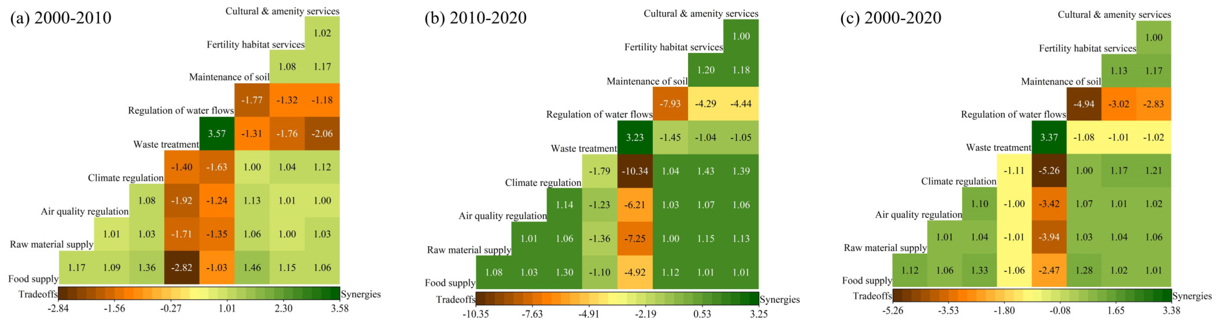
4.4. Analysis of Tradeoffs/Synergies Between ESs

A tradeoffs/synergies analysis was conducted on nine ESs (food supply, raw material supply, air quality regulation, climate regulation, waste treatment, regulation of water flows, maintenance of soil, fertility habitat services, cultural and amenity services) in the LCEB to quantify the interaction relationships among various ESs during the study period. The results indicate that the nine ESs formed a total of 36 data groups, with 22 groups showing positive values and 14 groups showing negative values, with synergies accounting for 61.11%, indicating that the dominant relationship among ESs during the study period was synergies (Figure 6). Synergies mainly existed among provisioning services, supporting services, and cultural services, as well as within these three services, and tradeoffs were most significant between the regulation of water flows and other ESs. From 2000 to 2010, the highest synergy was between waste treatment and regulation of water flows (3.57), and the lowest was between air quality regulation and cultural and amenity services (1.00). Significant tradeoffs were observed between the ES pairs of food supply and waste treatment and cultural and amenity services and waste treatment. Between 2010 and 2020, a pronounced tradeoff developed between climate regulation and water flow regulation (−10.34), alongside intensified tradeoffs between water flow regulation and both supporting and cultural services. The highest synergy value was between waste treatment and regulation of water flows (3.23). From 2000 to 2020, the tradeoffs and synergies were weaker, with smaller extreme values.

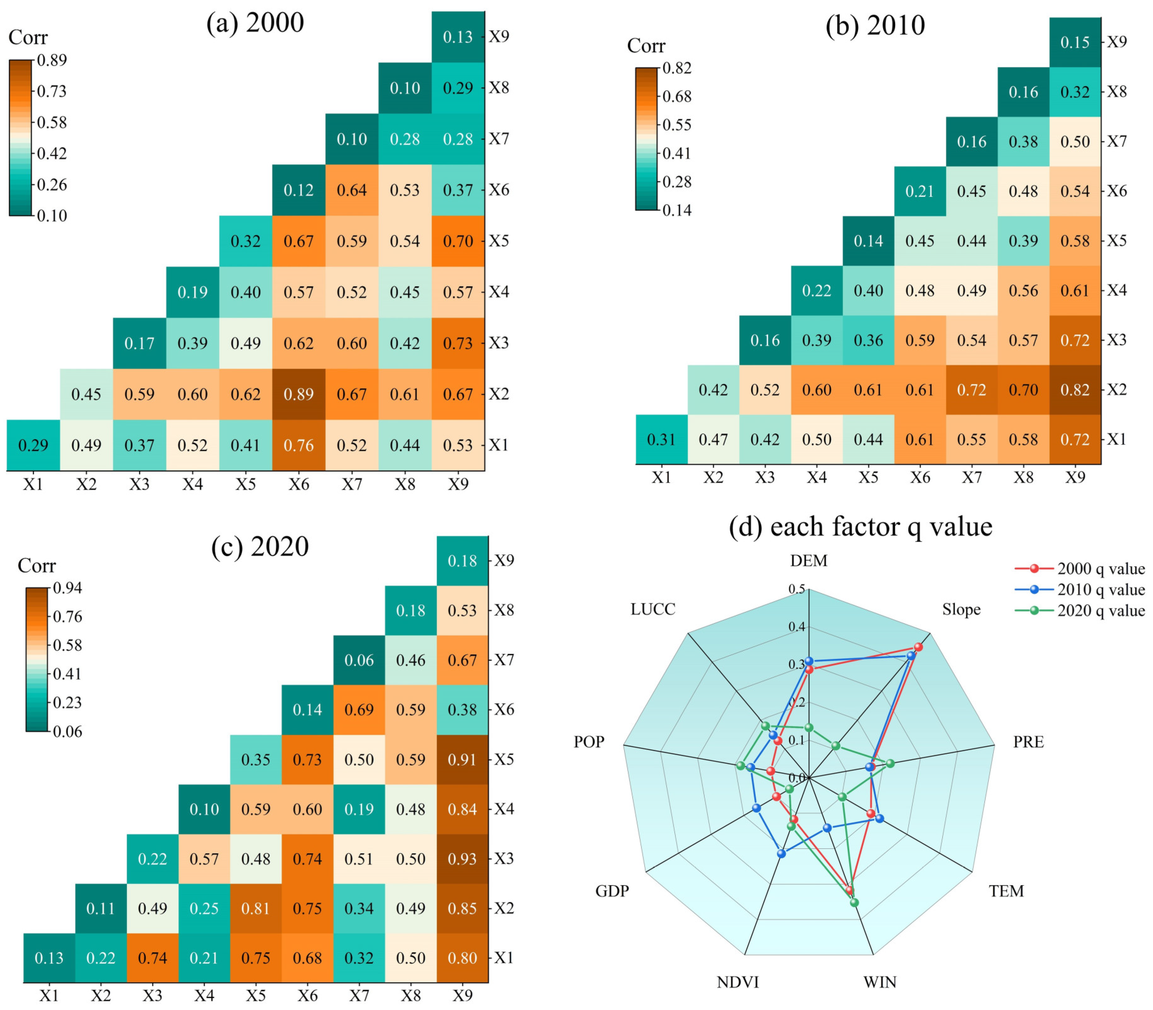
4.5. Spatial Heterogeneity of ESV

Within the framework of county (district) administrative units, the ESV was treated as the dependent variable, while nine natural and socio-economic factors served as independent variables. Geographic detection was performed to explore the main influencing factors of spatial differentiation of the ESV in the LCEB and the interactions among various driving factors. Utilizing the “Factor Detection” module within GeoDetector, the average explanatory power of each factor across the three periods ranked from high to low was as follows: Slope (0.33) > WIN (0.27) > DEM (0.24) > PRE (0.18) > TEM (0.17) > NDVI (0.16) > LUCC (0.15) > POP (0.15) > GDP (0.11). Therefore, topography and climate factors were the main driving factors of the ESV, while the impacts of GDP and POP were smaller, consistent with previous research findings [26,46].

The “Interaction Detection” quantified the nonlinear explanatory power arising from the coupling effects between factors on ESV variation, thereby adeptly discerning the synergistic and antagonistic influences of multiple drivers [47]. Our analysis demonstrated that the spatial differentiation of the ESV in the LCEB is marked by a robust dual-factor enhancement effect (Figure 7). Notably, every interaction pair’s q-value surpasses that of any single factor alone, underscoring the inherently nonlinear dynamics governing ESV evolution. This pronounced spatial heterogeneity in multi-scale driving forces underscores that variations in the coastal ESV are fundamentally shaped by the intertwined interplay of land–sea interactions, policy governance, and natural baseline conditions, all mediated through complex network effects. In 2000, the interaction between NDVI and slope had the greatest impact on the spatial heterogeneity of the ESV (0.89). In 2010, the interaction between LUCC and slope had the greatest impact on the spatial heterogeneity of the ESV (0.82). In 2020, the interactions between LUCC and PRE, as well as LUCC and WIN, both exceeded 0.90.

5. Discussion

5.1. ESV Responses to Land Use

This study highlights the marked sensitivity of ESVs to land use changes within the LCEB. Dominated by forest land and shallow water—which together contribute over 75% of the total ESV—their higher ESVs primarily arise from their crucial roles in climate regulation and food supply (Table 1). Notably, between 2000 and 2020, urban expansion drove a 51.9% loss of saltwater wetland (Table 2), leading to a direct reduction of 1.51 billion yuan in food supply services (Table 3). This pattern mirrors observations in rapidly urbanizing coastal regions such as the Pearl River Delta [48] and the Yangtze River Delta [28]. However, unlike those areas, the LCEB inland freshwater zones expanded by 61.3%, with increased regulation of water flow services partially offsetting the detrimental impacts of urban sprawl, creating a distinctive “freshwater compensation effect.”

ESVs have fluctuated over time, with their spatial centroids exhibiting varying degrees of shift. Analysis using the standard deviation ellipse reveals a consistent southwestward drift of the ESV centroid (Figure 5), spatially mirroring the expansion of freshwater in Yingkou and the degradation of forests in northern Dalian. This movement contrasts with the possible southeastward shift of the economic center, representing a “counter-directional dynamic” that underscores intensifying spatial transformations in the region, thereby affirming the common ecological–economic spatial contest observed throughout the Bohai Rim [49]. The Markov transition matrix indicates that transitions into grade 2 dominate, comprising roughly 50% of all changes (Table 4), predominantly concentrated in the coastal shelter forest enhancement zone between Huludao and Jinzhou. This highlights the pronounced effectiveness of ecological restoration efforts in rehabilitating low-value areas, a pattern comparable to that seen in the Jiaozhou Bay coastal zone [50].

Between 2010 and 2020, the intensification of tradeoffs between the regulation of water flows and climate regulation became particularly pronounced, revealing a complex interplay: while the expansion of freshwater bolstered the regulation of water flows, it may have simultaneously undermined climate regulation by altering local evapotranspiration dynamics. This phenomenon of “service competition” is similarly observed in the Poyang Lake region [42], underscoring the need for establishing service flow accounting mechanisms in critical areas like the Liaohe Estuary to strategically optimize wetland restoration spatially. Land use changes exert profound impacts on the tradeoffs between the regulation of water flows and climate regulation by modifying the physical attributes of surface cover and disrupting ecological processes. In rapidly urbanizing coastal zones, the increase in construction land elevates surface imperviousness, which, despite enhancing water purification through reduced non-point source pollution, markedly weakens runoff regulation and exacerbates urban heat island effects, thereby intensifying the tradeoffs between climate regulation and the regulation of water flows [51]. Meanwhile, in low-gradient coastal plains, intensive agriculture has depleted soil organic matter, and drainage infrastructure development has raised runoff coefficients, leading to notable tradeoffs between the regulation of water flows and maintenance of soil.

This study provides a comprehensive analysis of the temporal impacts exerted by both natural and socio-economic drivers on the ESV within the coastal region under investigation. It confirms that natural factors overwhelmingly govern the spatial distribution of the coastal ESV, whereas anthropogenic influences contribute relatively less to its spatial evolution. Topographical attributes, particularly slope and DEM, serve as pivotal determinants of ESV spatial heterogeneity. The Liaodong Mountain area, with its pronounced soil and water conservation capacity, consistently exhibits an elevated ESV, notably through the enhanced regulation of water flows and maintenance of soil within forested zones. In contrast, the Panjin wetlands stand out as a high-value ESV hotspot, a fact attributed to their significant contributions to the regulation of water flows and blue carbon sequestration. Climatic variables, including WIN and PRE, modulate the ESV primarily by affecting vegetation productivity; for instance, the central Huludao region, characterized by lower WIN and higher NDVI, corresponds to increased ESVs, whereas drier regions such as Panjin and Jinzhou, with sparser vegetation, display comparatively diminished ESVs. The dominance of topographic and climatic factors substantiates the foundational role of natural background conditions in shaping coastal ESV patterns. Nonetheless, the temporal evolution of driving factors reveals pronounced human–environment interactions: during 2000–2010, the interplay between NDVI and slope was predominant, indicating that topography constrained the ecological benefits derived from vegetation recovery. In 2020, the interactive surge of LUCC and climatic factors indicated that human activities in the study area had surpassed natural thresholds, becoming the dominant force in reshaping the landscape. This shift in the driving paradigm from “natural” to “anthropogenic” stands in contrast to the evolutionary trajectory of the Yangtze River Delta coastal zone [28], where the dominance of socio-economic factors may have emerged earlier. Furthermore, the study identifies the interaction between LUCC and precipitation as the strongest driving factor in 2020, suggesting that, under the context of climate change, altered precipitation patterns may exacerbate the conversion dynamics among farmland, freshwater, and wetlands by modulating agricultural water demand—a mechanism that remains underexplored in current coastal ecosystem research.

5.2. Complex Interactions Between ESs

Assessing tradeoffs/synergies between ESs is crucial for effective management decisions. The study found a significant synergy between waste treatment and the regulation of water flows, but both exhibited tradeoffs with other ESs. This is due to the high ESV provided by inland freshwater, which enhances the ESV of the regulation of water flows and waste treatment. The increase in water area regulates the climate of surrounding areas through precipitation, promoting vegetation growth, which in turn conserves water and soil, thus demonstrating a strong synergy between climate regulation and soil conservation and biodiversity.

Research to date on the tradeoffs and synergies among ESs has predominantly utilized spatial mapping and statistical analyses for qualitative characterization [52]. These conventional approaches inherently assume linear statistical relationships among diverse ESs, thereby inadequately capturing the intricate and multifaceted interactions that define these ecological functions. For example, the prevalent use of correlation coefficients presupposes monotonic relationships between ES pairs, limiting insight to generalized trends while overlooking critical nonlinear dynamics and complex multifactorial influences [25,53]. Considering that ecosystem processes are concurrently modulated by topographic features, climatic variables, and LUCC, reductive linear models fail to faithfully represent these complexities [54,55], frequently yielding outcomes that diverge from empirical realities.

To more precisely delineate the direction and intensity of interactions among ESs, this study adopted the ESTD model, grounded in data-driven linear fitting, to quantify the tradeoffs and synergy relationships. Distinct from traditional statistical methods, ESTD encompasses not only tradeoffs and synergies but also compatibility relationships, thereby unveiling more intricate patterns of interaction [56]. By computing the change indices of individual ESs and fitting these through linear models, ESTD affords a nuanced and comprehensive appraisal of their interdependencies, transcending the constraints of linear assumptions and fully integrating the multifaceted influences at play [42]. As such, ESTD excels in capturing both the direction and magnitude of ES interactions, offering robust, efficient, and insightful support for resource management and policy decisions.

5.3. Policy Suggestions

Based on the research findings, forest land and shallow water are vital contributors to the ESV. In contrast, the natural ecological space, such as farmland, grassland, and shallow water, continues to decline in proportion to coastal ESs. Therefore, it is recommended that spatial planning for the coastal zone should delineate clear ecological red-line areas to protect ecological integrity and ensure its service functions are not threatened. Additionally, by integrating geographic information system (GIS) technology, dynamic monitoring of changes in ESVs should be conducted, with timely adjustments to spatial planning strategies to adapt to ecological environmental changes. Given the significant tradeoffs between the regulation of water flows and other ESs, prioritizing the regulation of water flows in water resource management is advised. By establishing a watershed management mechanism that comprehensively considers hydrological, ecological, and socio-economic factors, scientifically formulated water resource allocation plans can be developed to enhance hydrological regulation capacity and ensure ecosystem health. The explanatory power of natural factors on the spatial changes of the ESV in the LCEB is greater than that of socio-economic factors, and the interactions between different driving factors are greater than the impact of any single factor. It is recommended that decision-makers regularly conduct dynamic assessments of ESVs, combining remote sensing monitoring and geographic detector analysis, considering evaluation results at different spatial and temporal scales to identify critical factors influencing ESVs. This offers a robust scientific foundation for informed policy-making, thereby enhancing the precision, efficacy, and contextual relevance of subsequent management interventions.

5.4. Research Limitations and Perspectives

This study offers valuable insights into the spatiotemporal evolution of ESVs and introduces a novel approach for assessing ESV responses to LUCC. The insights gained herein hold significant implications for the evidence-based and adaptive management of future ecological systems. Nevertheless, it is important to note that the ESV in the study area is directly influenced by land use extent, and the accuracy of ESV estimates depend heavily on the precision of land use classification data. Future research could combine artificial intelligence and machine learning methods to obtain higher precision land use classification data to improve research accuracy [57]. The application of GeoDetector for driving discretization currently needs more standardization, and different methods may yield varying results, potentially affecting research precision. Furthermore, based on existing research conditions, the 5 km × 5 km regular grid established in this study could be further refined to improve the spatiotemporal visualization of research results.

6. Conclusions

This study systematically examined the spatiotemporal dynamics of the ESV and the associated tradeoffs and synergies among ESs in the LCEB over the period of 2000 to 2020, utilizing a modified equivalent factor table. By leveraging the GeoDetector model, it further identified the dominant drivers underlying ESV variations, offering a novel analytical framework for understanding their evolution. The findings provide rigorous scientific support for regional ecological management and the formulation of evidence-based environmental policies. The following conclusions can be made: (1) The ESV in the LCEB exhibited a fluctuating characteristic of decline followed by an increase. During the study period, forest land and shallow water remained the dominant contributors to the overall ESV. The expansion of inland freshwater areas was the principal driver behind the observed increase in the ESV. (2) Areas with high ESVs were predominantly located in regions rich in water resources, whereas lower ESVs were concentrated primarily in central and coastal zones. Moreover, coastal regions undergoing rapid economic development exhibited more pronounced variability and fluctuations in their ESV levels. (3) During the study period, the dominant relationship among ESs was synergy, with tradeoffs being most significant between waste treatment and other ESs. (4) Topography and climate factors were the primary drivers of spatial heterogeneity in the ESV, with interactions between any two selected factors exceeding the impact of a single factor.

References

1. Liu, L.; Wu, J. Space Cannot Substitute for Time in the Study of the Ecosystem Services-Human Wellbeing Relationship. Geogr. Sustainability 2025, 6, 100221. [Google Scholar] [CrossRef]
2. Daily, G.C. Nature’s Service: Societal Dependence Onnatural Ecosystems; Island Press: Washington, DC, USA, 1997. [Google Scholar]
3. Yuan, L.; Geng, M.; Li, F.; Xie, Y.; Tian, T.; Chen, Q. Spatiotemporal Characteristics and Drivers of Ecosystem Service Interactions in the Dongting Lake Basin. Sci. Total Environ. 2024, 926, 172012. [Google Scholar] [CrossRef]
4. Zhu, C.; Chen, Y.; Wan, Z.; Chen, Z.; Lin, J.; Chen, P.; Sun, W.; Yuan, H.; Zhang, Y. Cross-Sensitivity Analysis of Land Use Transition and Ecological Service Values in Rare Earth Mining Areas in Southern China. Sci. Rep. 2023, 13, 22817. [Google Scholar] [CrossRef]
5. Xie, G.; Zhen, L.; Lu, C.; Xiao, Y.; Chen, C. Expert knowledge based valuation method of ecosystem services in China. J. Nat. Rescour. 2008, 154, 911–919. [Google Scholar]
6. Xie, G.; Zhang, C.; Zhen, L.; Zhang, L. Dynamic Changes in the Value of China’s Ecosystem Services. Ecosyst. Serv. 2017, 26, 146–154. [Google Scholar] [CrossRef]
7. Wang, J.; Lai, X.; Zhang, Z.; Zhou, S.; Lv, L.; Fan, Y. Optimization of Territorial Ecological Space under the Constraint of Ecosystem Service Externalities. Ecol. Indic. 2024, 168, 112752. [Google Scholar] [CrossRef]
8. Guo, P.; Zhang, F.; Wang, H. The Response of Ecosystem Service Value to Land Use Change in the Middle and Lower Yellow River: A Case Study of the Henan Section. Ecol. Indic. 2022, 140, 109019. [Google Scholar] [CrossRef]
9. Zhang, L.; Yu, K.; Zhang, Y.; Wei, J.; Yang, W.; Wang, X. Research on the Value of County-Level Ecosystem Services in Highly Mountainous Canyon Areas Based on Land Use Change: Analysis of Spatiotemporal Evolution Characteristics and Spatial Stability. Land 2025, 14, 398. [Google Scholar] [CrossRef]
10. Gong, J.; Liu, D.; Zhang, J.; Xie, Y.; Cao, E.; Li, H. Tradeoffs/Synergies of Multiple Ecosystem Services Based on Land Use Simulation in a Mountain-Basin Area, Western China. Ecol. Indic. 2019, 99, 283–293. [Google Scholar] [CrossRef]
11. Wang, X.; Lu, B.; Li, J.; Liu, Q.; He, L.; Lv, S.; Yu, S. Spatio-Temporal Analysis of Ecological Service Value Driven by Land Use Changes: A Case Study with Danjiangkou, Hubei Section. Resour. Environ. Sustain. 2024, 15, 100146. [Google Scholar] [CrossRef]
12. Wang, K.; Jia, M.; Zhang, X.; Zhao, C.; Zhang, R.; Wang, Z. Evaluating Ecosystem Service Value Changes in Mangrove Forests in Guangxi, China, from 2016 to 2020. Remote Sens. 2024, 16, 494. [Google Scholar] [CrossRef]
13. Ye, Q.; Tian, G.; Liu, G.; Ye, J.; Yao, X.; Liu, Q.; Lou, W.; Wu, S. Tupu Methods of Spatial-Temporal Pattern on Land Use Change: A Case Study in the Yellow River Delta. J. Geogr. Sci 2004, 14, 131–142. [Google Scholar]
14. Zhang, L.; Hu, B.; Zhang, Z.; Liang, G. Research on the Spatiotemporal Evolution and Mechanism of Ecosystem Service Value in the Mountain-River-Sea Transition Zone Based on “Production-Living-Ecological Space”—Taking the Karst-Beibu Gulf in Southwest Guangxi, China as an Example. Ecol. Indic. 2023, 148, 109889. [Google Scholar] [CrossRef]
15. Dang, L.; Zhao, F.; Teng, Y.; Teng, J.; Zhan, J.; Zhang, F.; Liu, W.; Wang, L. Scale Dependency of Trade-Offs/Synergies Analysis of Ecosystem Services Based on Bayesian Belief Networks: A Case of the Yellow River Basin. J. Environ. Manage. 2025, 375, 124410. [Google Scholar] [CrossRef]
16. Dai, E.; Wang, X.; Zhu, J.; Zhao, D. Methods, Tools and Research Framework of Ecosystem Service Trade-Offs. Geogr. Res. 2016, 35, 1005–1016. [Google Scholar]
17. Howe, C.; Suich, H.; Vira, B.; Mace, G.M. Creating Win-Wins from Trade-Offs? Ecosystem Services for Human Well-Being: A Meta-Analysis of Ecosystem Service Trade-Offs and Synergies in the Real World. Glob. Environ. Change 2014, 28, 263–275. [Google Scholar] [CrossRef]
18. Zheng, Y.; Yang, H.; Gong, H.; Shi, J.; Zhang, Y.; Wang, J.; Zhang, X.; Cheng, R.; Chen, Y. Spatiotemporal Changes and Trade-Offs/Synergies of Waterfront Ecosystem Services Globally. Sustainability 2025, 17, 472. [Google Scholar] [CrossRef]
19. Zhou, J.; Yang, J.; Tang, Z.; Xue, L.; Zhang, W.; Zhang, J. Driving Mechanisms of Ecosystem Services and Their Trade-Offs and Synergies in the Transition Zone between the Qinghai-Tibet Plateau and the Loess Plateau. Ecol. Indic. 2025, 171, 113148. [Google Scholar] [CrossRef]
20. Deng, X.; Li, Z.; Gibson, J. A Review on Trade-off Analysis of Ecosystem Services for Sustainable Land-Use Management. J. Geogr. Sci. 2016, 26, 953–968. [Google Scholar] [CrossRef]
21. Wang, Q.; Wang, L.; Wu, Q.; Du, P. Analysis of Spatial and Temporal Evolution of Ecosystem Service Value Based on the Framework of “Risk-Association-Driver”: A Case Study of Panjin City. Sustainability 2025, 17, 2950. [Google Scholar] [CrossRef]
22. Ding, X.; Jian, S. Synergies and Trade-Offs of Ecosystem Services Affected by Land Use Structures of Small Watershed in the Loess Plateau. J. Environ. Manag. 2024, 350, 119589. [Google Scholar] [CrossRef] [PubMed]
23. Wang, J.; Wu, W.; Yang, M.; Gao, Y.; Shao, J.; Yang, W.; Ma, G.; Yu, F.; Yao, N.; Jiang, H. Exploring the Complex Trade-Offs and Synergies of Global Ecosystem Services. Environ. Sci. Ecotechnol. 2024, 21, 100391. [Google Scholar] [CrossRef]
24. Li, Q.; Jia, Y.; Wang, H.; Wang, Z. Analysis of Trade-off and Synergy Effects of Ecosystem Services in Hebei Province from the Perspective of Ecological Function Area. ACTA Geogr. Sin. 2023, 78, 2833–2849. [Google Scholar]
25. Li, Y.; Luo, H. Trade-off/Synergistic Changes in Ecosystem Services and Geographical Detection of Its Driving Factors in Typical Karst Areas in Southern China. Ecol. Indic. 2023, 154, 110811. [Google Scholar] [CrossRef]
26. Xiao, J.; Song, F. Quantifying the Independent Contributions of Climate and Land Use Change to Ecosystem Services. Ecol. Indic. 2023, 153, 110411. [Google Scholar] [CrossRef]
27. Liu, S.; Zhang, P.; Jiang, X.; Lo, K. Measuring Sustainable Urbanization in China: A Case Study of the Coastal Liaoning Area. Sustain. Sci. 2013, 8, 585–594. [Google Scholar] [CrossRef]
28. Li, C.; Fang, S.; Geng, X.; Yuan, Y.; Zheng, X.; Zhang, D.; Li, R.; Sun, W.; Wang, X. Coastal Ecosystem Service in Response to Past and Future Land Use and Land Cover Change Dynamics in the Yangtze River Estuary. J. Cleaner Prod. 2023, 385, 135601. [Google Scholar] [CrossRef]
29. Yu, D.; Hao, R. Research Progress and Prospect of Ecosystem Services. Adv. Earth Sci. 2020, 35, 804. [Google Scholar]
30. Chuai, X.; Huang, X.; Wu, C.; Li, J.; Lu, Q.; Qi, X.; Zhang, M.; Zuo, T.; Lu, J. Land Use and Ecosystems Services Value Changes and Ecological Land Management in Coastal Jiangsu, China. Habitat Int. 2016, 164–174. [Google Scholar] [CrossRef]
31. Wang, X.; Bao, Y. Study on the Methods of Land Use Dynamic Change Research. Prog. Geogr. 1999, 18, 81–87. [Google Scholar]
32. Li, D.; Zhou, J.; Zhan, D. Spatial and Temporal Changes and Driving Factors of Cultivated Land in Heilongjiang Province. Sci. Geogr. Sin. 2021, 41, 1266–1275. [Google Scholar]
33. Xiao, J.; Qian, B.; Chen, G.; Shi, F.; Cao, X.; Zhu, C. Land Use Change and Evolution of Ecosystem Service Value in Maduo County of Source Region of the Yellow River. Acta Ecol. Sin. 2020, 40, 510–521. [Google Scholar]
34. Zhuang, D.; Liu, J. Study on the Model of Regional Differentiation of Land Use Degree in China. J. Nat. Resour. 1997, 12, 105–111. [Google Scholar]
35. Costanza, R.; De Groot, R.; Sutton, P.; Van der Ploeg, S.; Anderson, S.J.; Kubiszewski, I.; Farber, S.; Turner, R.K. Changes in the Global Value of Ecosystem Services. Glob. Environ. Change 2014, 26, 152–158. [Google Scholar] [CrossRef]
36. Mayila, R.; Mamat, S.; Nigela, T.; Yikiliman, A.; Ma, C.; Yierxiati, A. The Ecosystem Service Value Spatial-Temporal Changes in the Ugan-Kuqa River Delta Oasis Based on RS and GIS. Acta Ecol. Sin. 2018, 38, 5938–5951. [Google Scholar]
37. Li, Z.; Adam, N.A.; Mirzaliev, S.; Saydullaev, S.; Bai, H. An Integrated Approach for Evaluating the Spatial and Temporal Dynamics of Ecosystem Services and Ecological Risk Urban Agglomerations in China. Ecol. Indic. 2025, 172, 113248. [Google Scholar] [CrossRef]
38. Chen, B.; Liu, X.; Liu, J. Construction and Optimization of Ecological Security Patterns in Chinese Black Soil Areas Considering Ecological Importance and Vulnerability. Sci. Rep. 2025, 15, 12142. [Google Scholar] [CrossRef]
39. Xie, L.; Xu, J.; Zang, J.; Huang, T. Simulation and Prediction of Land Use Change in Guangxi Based on Markov-FLUS Model. Res. Soil Water Conserv. 2022, 29, 249–254. [Google Scholar]
40. Yang, Y.; Qin, T.; Yan, D.; Liu, S.; Feng, J.; Wang, Q.; Liu, H.; Gao, H. Analysis of the Evolution of Ecosystem Service Value and Its Driving Factors in the Yellow River Source Area, China. Ecol. Indic. 2024, 158, 111344. [Google Scholar] [CrossRef]
41. Lefever, D.W. Measuring Geographic Concentration by Means of the Standard Deviational Ellipse. Am. J. Sociol. 1926, 32, 88–94. [Google Scholar] [CrossRef]
42. Wen, Y.; Zhang, X.; Wei, J.; Wang, X.; Cai, Y. Temporal and Spatial Variation of Ecosystem Service Value and Its Trade-Offs and Synergies in the Peripheral Region of the Poyang Lake. Sci. Geogr. Sin. 2022, 42, 1229–1238. [Google Scholar]
43. Li, J.; Ren, Z.; Liu, Y.; Zhang, J. Tradeoffs-synergies Analysis among Ecosystem Services in Northwestern Valley Basin: Taking Yinchuan Basin as an Example. J. Desert Res. 2016, 36, 1731–1738. [Google Scholar]
44. Wang, J.; Xu, C.D. Geodetector: Principle and Prospective. Acta Geogr. Sin. 2017, 72, 116–134. [Google Scholar]
45. Zhang, X.; Yin, Q.; Zheng, Z.; Sun, S.; Huang, J. Dynamic Changes and Key Drivers of Ecosystem Service Values in Populous Zones on the Tibetan Plateau: A 35-Year Analysis. Ecol. Indic. 2024, 167, 112620. [Google Scholar] [CrossRef]
46. Yao, Y.; Song, Y.; Xue, Y.; Jian, C.; Wang, Z.; Zhang, G. Spatial-Temporal Variations and Mechanism of Ecosystem Services Value from Land Ues Perspective: A Case Study of Liaoning Coastal Zones. Areal Res. Dev. 2024, 43, 153–159. [Google Scholar]
47. Xia, H.; Yuan, S.; Prishchepov, A.V. Spatial-Temporal Heterogeneity of Ecosystem Service Interactions and Their Social-Ecological Drivers: Implications for Spatial Planning and Management. Resour. Conserv. Recycl. 2023, 189, 106767. [Google Scholar] [CrossRef]
48. Huang, Z.; Chen, Y.; Zheng, Z.; Wu, Z. Spatiotemporal Coupling Analysis between Human Footprint and Ecosystem Service Value in the Highly Urbanized Pearl River Delta Urban Agglomeration, China. Ecol. Indic. 2023, 148, 110033. [Google Scholar] [CrossRef]
49. Liu, Y.; Hou, X.; Li, X.; Song, B.; Wang, C. Assessing and Predicting Changes in Ecosystem Service Values Based on Land Use/Cover Change in the Bohai Rim Coastal Zone. Ecol. Indic. 2020, 111, 106004. [Google Scholar] [CrossRef]
50. Wan, L.; Wang, X.H.; Wu, W. Assessment of coastal eco- environmental sustainable development under multiple pressures: A Case Study of Jiaozhou Bay, China. J. Environ. Manag. 2024, 363, 121230. [Google Scholar] [CrossRef]
51. Lian, L.; Li, B.; Chen, Z.; Chen, Y.; Sun, X. Quantifying the climatic and hydrological effects of land use/cover change based on Weather Research and Forecasting model. Acta Ecol. Sin. 2018, 38, 917–925. [Google Scholar]
52. Wang, Y.; Cheng, H.; Wang, N.; Huang, C.; Zhang, K.; Qiao, B.; Wang, Y.; Wen, P. Trade-off and Synergy Relationships and Spatial Bundle Analysis of Ecosystem Services in the Qilian Mountains. Remote Sens. 2023, 15, 2950. [Google Scholar] [CrossRef]
53. Xiong, C.; Ren, H.; Xu, D.; Gao, Y. Spatial Scale Effects on the Value of Ecosystem Services in China’s Terrestrial Area. J. Environ. Manag. 2024, 366, 121745. [Google Scholar] [CrossRef] [PubMed]
54. Li, Q.; Li, W.; Wang, S.; Wang, J. Assessing Heterogeneity of Trade-Offs/Synergies and Values among Ecosystem Services in Beijing-Tianjin-Hebei Urban Agglomeration. Ecol. Indic. 2022, 140, 109026. [Google Scholar] [CrossRef]
55. Bennett, E.M.; Peterson, G.D.; Gordon, L.J. Understanding Relationships among Multiple Ecosystem Services. Ecol. Lett. 2009, 12, 1394–1404. [Google Scholar] [CrossRef] [PubMed]
56. Cord, A.F.; Bartkowski, B.; Beckmann, M.; Dittrich, A.; Hermans-Neumann, K.; Kaim, A.; Lienhoop, N.; Locher-Krause, K.; Priess, J.; Schröter-Schlaack, C.; et al. Towards Systematic Analyses of Ecosystem Service Trade-Offs and Synergies: Main Concepts, Methods and the Road Ahead. Ecosyst. Serv. 2017, 28, 264–272. [Google Scholar] [CrossRef]
57. Yan, E.P.; Lin, H.; Wang, G.X.; Xia, C. Analysis of Evolution and Driving Force of Ecosystem Service Values in the Three Gorges Reservoir Region during 1990–2011. Acta Ecol. Sin. 2014, 34, 5962–5973. [Google Scholar]
Figure 1. Location of the study area. The standard map production is based on the GS (2024) 0650 standard of the Ministry of Natural Resources map service website.
Sustainability 17 05245 g001
Figure 2. Spatiotemporal distribution of ESV in LCEB.
Sustainability 17 05245 g002
Figure 3. ESV levels transition Tupu units in the LCEB. The numbers within the chart indicate transitions between ESV levels; for instance, “11” denotes a transition from Level 1 to Level 1, with similar notation applying to other level changes.
Sustainability 17 05245 g003
Figure 4. Rising and falling Tupu of ESV levels of LCEB.
Sustainability 17 05245 g004
Figure 5. Elliptical variation of ESV standard deviation of LCEB.
Sustainability 17 05245 g005
Figure 6. Tradeoffs/synergies of multiple ESs of LCEB.
Sustainability 17 05245 g006
Figure 7. Driving forces of socio-ecological factors. Note: X1: DEM, X2: Slope, X3: PRE, X4: TEM, X5: WIN, X6: NDVI, X7: GDP, X8: POP, X9: LUCC.
Sustainability 17 05245 g007