A Stochastic Knapsack Model for Sustainable Safety Resource Allocation Under Interdependent Safety Measures

Abstract

The optimum choice of safety measures (SMs) within constraints is necessary for effective risk management in occupational health and safety (OHS). The stochastic nature of safety interventions is frequently overlooked by traditional approaches such as deterministic models and risk matrices. This study presents a novel stochastic knapsack model that maximizes the overall expected benefit during a risk assessment period considering budgetary constraints and the interdependencies between risks and safety measures. Two models are developed as follows: a one-to-one relationship model assuming independent risks and a multiple-relationship model accounting for interdependent safety measures. The suggested model’s real-world implementation is illustrated through a case study in the retail industry. The results demonstrate the model’s ability to efficiently prioritize SMs, showing an 18% reduction in objective function value and an average risk reduction of 29.5 per monetary unit invested, compared to 26.2 for the deterministic model. A more realistic and flexible framework for safety investment planning is offered by the analysis, which emphasizes the benefits of including stochastic components and interdependencies in decision-making. By addressing the significant drawbacks of deterministic models and providing a flexible, data-driven framework for safety optimization, this study adds to the body of literature. The suggested model is in line with the United Nations Sustainable Development Goals (SDGs), specifically SDGs 3, 8, 9, and 12. Its adaptability contributes to achieving SDG 13, emphasizing possible uses in risk management for climate change. This study shows how decision-making that is structured and aware of uncertainty can support safer, more sustainable industrial processes.

1. Introduction

In today’s industrial landscape, effective safety management is essential for preventing workplace hazards and reducing potential financial and human losses. However, the challenge lies in selecting the most effective safety measures (SMs) given the inherent uncertainty of risk factors and limited resources. Traditional risk management methods, such as risk matrices, while widely used for their simplicity, often fall short in adequately addressing complex interdependencies between risks and the stochastic impacts of SMs.

Current risk assessment methods either rely on qualitative judgments or quantitative models that treat the impacts of SMs as deterministic. However, real-world scenarios often reveal that implementing SMs can lead to unpredictable outcomes—sometimes reducing risks, sometimes having no effect, and occasionally exacerbating the hazard. This unpredictability highlights the need for a more nuanced approach to optimize safety investments under uncertainty.

This study presents a novel solution to this problem: a stochastic knapsack model designed to integrate risk matrices with SM selection under budget constraints. Unlike deterministic models, our approach accounts for the stochastic nature of SMs’ impact, providing a more flexible and realistic decision-making tool. By introducing this model, we aim to fill a significant gap in the literature, as existing models overlook the probabilistic outcomes of safety interventions.

The proposed model—initially focused on straightforward one-to-one relationships between risks and SMs and subsequently expanded to encompass multiple, interdependent SMs—provides decision-makers with a practical framework for maximizing expected returns on safety investments. The applicability of the expanded model is demonstrated through a real-world example in Section 3.3, showcasing its effectiveness in optimizing investments in SMs within resource-constrained environments.

2. Literature Review

Hazard refers to a condition with the potential to cause harm, injury, or loss, while risk combines the probability of a hazardous event with its severity [1,2,3,4]. Managing workplace risks is vital for minimizing losses and ensuring safety, necessitating systematic approaches to risk assessment and control [5,6,7,8]. Effective risk management identifies risks, evaluates their impacts, and prioritizes resources to mitigate them efficiently [9,10]. Ensuring workplace safety while optimizing resource allocation supports sustainable development by promoting the achievement of the Sustainable Development Goals (SDGs) that emphasize the importance of workplace health and safety (SDG 3), economic productivity (SDG 8), sustainable industrialization (SDG 9), sustainable consumption patterns (SDG 12), and climate action (SDG 13) [11]. The SDGs addressed by this study’s contributions are presented in

Table 1. Relevant SDGs and their associated goals.

SDG No	Short Description	Goal
3	Good Health and Well-Being	Ensure healthy lives and promote well-being for all at all ages
8	Decent Work and Economic Growth	Promote sustained, inclusive, and sustainable economic growth, full and productive employment, and decent work for all
9	Industry, Innovation, and Infrastructure	Build resilient infrastructure, promote inclusive and sustainable industrialization, and foster innovation
12	Responsible Consumption and Production	Ensure sustainable consumption and production patterns
13	Climate Action	Take urgent action to combat climate change and its impacts

.

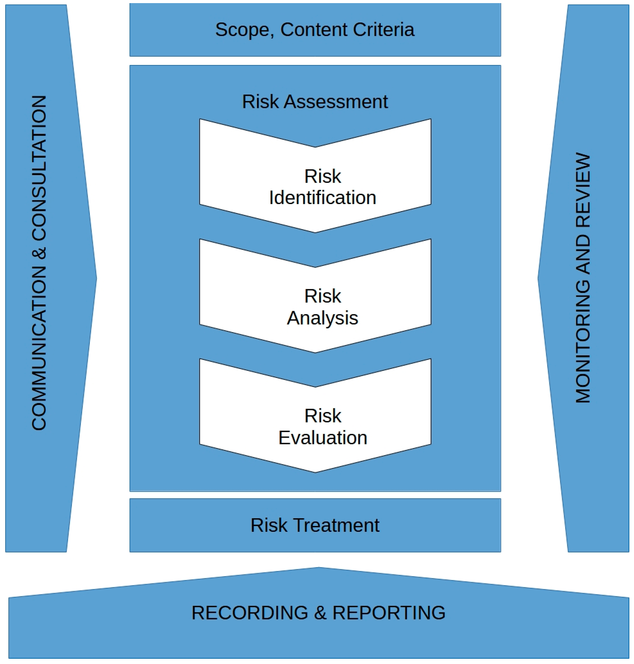
2.1. Risk Assessment Process and Methods

Risk assessment is a structured process critical to risk management, comprising hazard identification, risk analysis, and the implementation of control measures [12,13,14,15]. The risk management process as depicted by ISO 31000 [14] is illustrated in Figure 1. This process is typically guided by principles such as prioritizing collective protection over personal protection, avoiding additional risks during implementation, finding solutions tailored to specific organizational needs, and preferring control measures that provide the highest degree of protection with the least expenditure [16,17,18]. It is also essential to recognize that risks and control methods vary across organizations and are perceived differently based on the characteristics and perspectives of assessors [18,19,20,21,22].

Risk matrices are among the most popular risk assessment methods. They allow for both qualitative and quantitative applications, relying on subjective judgments and numerical data, respectively [23,24,25,26,27].

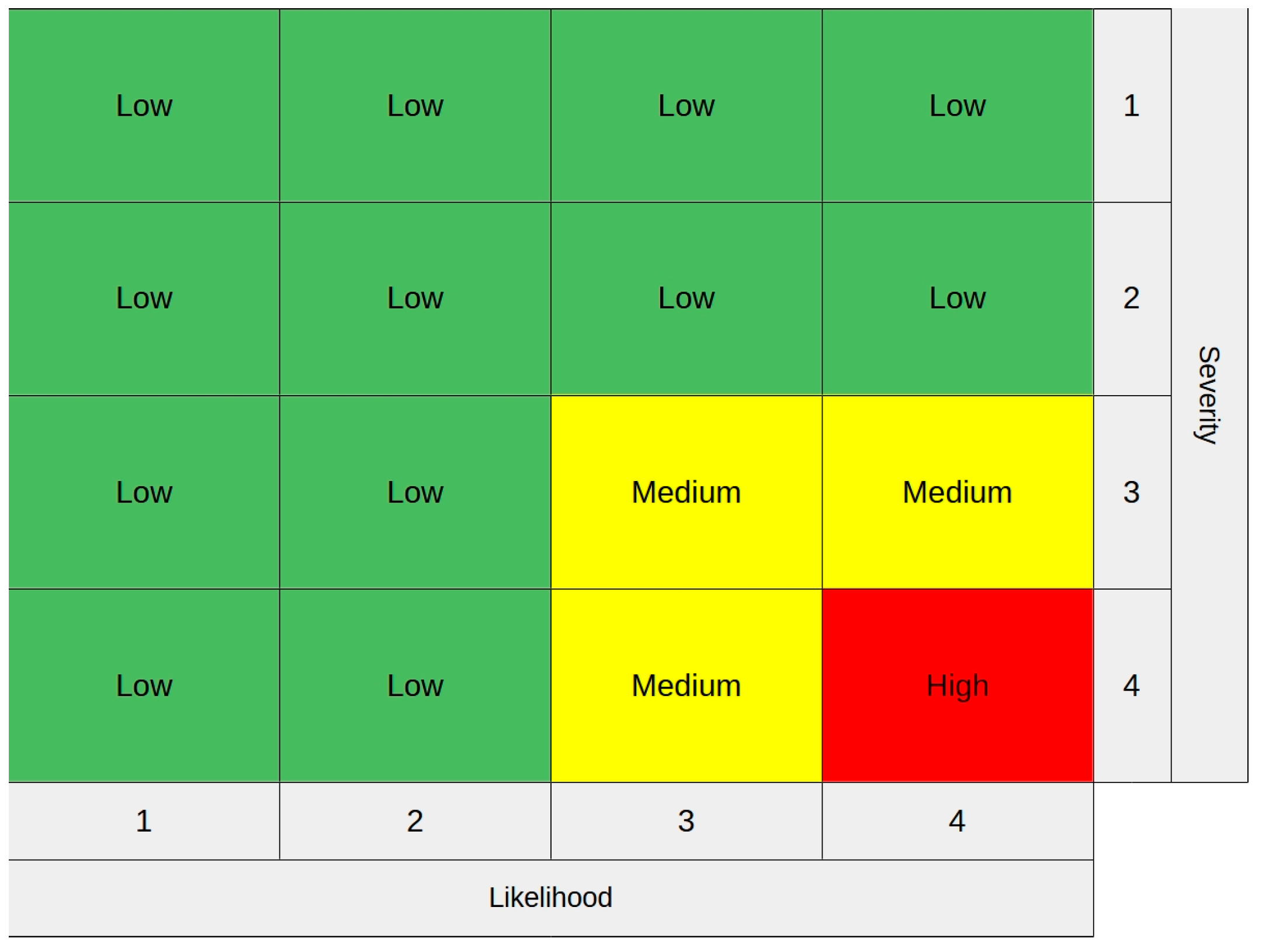
2.2. Risk Matrices and Their Limitations

Risk matrices are tools widely used for risk assessment, offering a simple and effective means of classifying risks and guiding decision-making [9,22,24,28,29,30,31]. They enable visually representing risks through a grid format, allowing stakeholders to communicate, prioritize, and allocate resources effectively [24,26]. Despite their simplicity, several limitations undermine their robustness, especially under conditions of uncertainty.

Risk matrices have been successfully utilized in various fields, including production [32], manufacturing [33,34,35], medicine [36,37,38], construction [39,40,41], aviation [42,43], railways [44,45], agriculture [38,46], and mining [10,47,48,49]. Risk matrices assist decision-makers in focusing on high-priority risks and provide consistency in prioritizing risks [1,21,24,50].

Risk matrices are often presented as tables classifying risks into severity and likelihood levels [30,51,52,53,54]. While there is no universally prescribed number of likelihood and severity levels, a 4 × 4 grid structure is typically used, as shown in Figure 2 [7,55,56].

In general, risks are categorized into green (low risk), yellow (medium risk), and red (high risk) regions, enabling appropriate resource allocation to mitigate higher-priority risks [53,56,57].

To accurately position risks in the matrix, both probability and severity values are needed [20,24,28,58,59,60]. The algebraic product of probability and severity approximates risk, aligning with its quantitative definition [53,58]. Qualitative risk matrices often multiply ordinal levels of probability and severity for simplicity: for example, the risk score for the red region in Figure 2 is 4 × 4 = 16. On the other hand, quantitative approaches use precise probabilities and monetary severity values to compute expected risk levels over a set period [61,62,63,64].

Table 2. Severity and likelihood scales.

Scale	Severity (in Monetary Units/Period)		Scale	Likelihood (/Period)
1	Negligible	<10,000	1	Impossible	<0.001
2	Marginal	[10,000; 100,000)	2	Improbable	[0.001; 0.01)
3	Critical	[100,000; 1,000,000)	3	Occasional	[0.01; 0.1)
4	Catastrophe	[1,000,000; 10,000,000]	4	Frequent	[0.1; 1]

presents typical values for quantitative risk matrices. For example, if the likelihood is 2 and the severity is 3, the expected risk level for the corresponding cell can be estimated by multiplying the midpoints of their ranges: 0.0055 × 550,000 = 3025 monetary units per period.

One major issue with risk matrices is the subjectivity inherent in assigning severity and likelihood levels. Experts often rely on personal judgment, which can be influenced by biases, varying experiences, and inconsistent definitions of scale categories [24,30,59]. This subjectivity leads to discrepancies in risk rankings, where risks of differing magnitudes may be assigned similar levels, or vice versa, resulting in risk ranking reversals [1,20,24,65]. While logarithmic scales and re-zoning techniques have been proposed for mitigating these issues, they offer only partial solutions to the problem [1,24,58]. Furthermore, risk matrices may not be effective when likelihood and severity are negatively correlated [53].

Uncertainty is another critical factor. Risk matrices often use ranges to estimate severity and likelihood levels in a discretized fashion, introducing ambiguity and reducing precision [1,24,31,66]. Approaches such as fuzzy logic and continuous scales have been suggested to address these uncertainties, but their implementation is resource-intensive and requires additional expertise [24,31].

2.3. Probability Estimation via Expert Judgment

When data are limited, occupational health and safety (OHS) practitioners rely on judgmental inputs, which can be quantified through various methods, including arithmetic or geometric pooling, Bayesian approaches, and Cooke’s classical method [67,68,69,70]. Risk matrices, supported by experts’ inputs, rank risks based on intuition and experience [30,70,71].

There are methods for eliciting probabilities from individual experts, such as direct estimation, betting scenarios, and lottery comparisons, but these approaches are inherently subjective, incorporating an expert’s value judgments [69,72].

Group judgments often outperform individual assessments when group members make independent decisions, are decentralized, possess diverse knowledge about the issue at hand, and have a methodology for combining their judgements [73,74,75]. Aggregation methods, such as averaging, often outperform complex techniques in combining expert judgments effectively [70,76]. Moreover, some mathematical transformations have been proposed for applications to average probability forecasts to compensate for over-estimation and under-estimation biases [75,77]. Practical methods, such as simple averaging, remain widely used due to their ease of implementation and consistent performance across scenarios [78]. These methods enable practitioners to estimate hazard likelihoods, severities, and SM impact probabilities, which are addressed further in Section 2.4.

2.4. SM Impact Probability

Previous studies have assumed that the impacts of SMs are deterministic, that is, applying an SM results in a certain decrease in the risk level, while not applying an SM does not change the risk level. However, this may not hold true in real-life scenarios.

According to Yuan et al. [79], SMs are categorized as inherent, engineered, and procedural. The efficacy of procedural SMs is contingent upon human factors, including the effectiveness of safety training and the response time of the operator.

Moreover, the efficacy of an SM is diminished when other SMs contribute to reducing the same hazard. Furthermore, the greater the overall risk reduction, the more challenging it becomes to achieve additional risk reduction through an SM. This finding is in line with the law of diminishing marginal returns [80].

The deployment of new SMs may lead to an increase in risk-taking behavior among individuals. In the absence of such consideration, the planned SMs may have either no effect or a negative effect on safety. Furthermore, investment in a new SM may reduce the resources that could otherwise be allocated to other planned SMs. In this case, the reallocation of resources may result in the SM becoming less effective than anticipated. Even in the absence of behavioral change among the company’s employees, the situation may have a negative effect on safety [81].

Individual differences also play a role: experts incorporate their attitudes into evaluating risk. In the case of a pessimistic expert, the risk scores assigned are typically higher than the objective risk score. Conversely, in the case of an optimistic expert, the risk scores are typically lower than the objective risk score [82]. Further, the background knowledge of the assessor impacts the results of risk assessment. Depending on the background knowledge of the assessor, the predictions made may be either accurate or inaccurate under real-life conditions. While processing risk assessment data, it is important to consider the uncertainty that may arise due to the assessor’s background knowledge [18].

Implementing an SM may or may not influence the risk level. Similarly, if no SM is implemented, the situation may remain unchanged or even worsen, increasing the risk. Consequently, the effects of SMs should be evaluated, since they might have lower-than-intended effects or unexpected negative effects on system safety [18]. It can be stated that the impacts of the SMs are stochastic, as these situations may occur with certain probabilities [83].

This study assumes that the impacts of the SMs are stochastic. In the simple one-to-one relationship scenario, the SMs are assumed to work independently of each other, allowing for their implementation without affecting other SMs. The independence of SMs can be realistic if risk reduction resources are distributed among disassociated, non-interacting locations or facilities [83]. Selecting an SM to mitigate a risk may improve the condition and reduce the risk with a probability of ρ, or it may not affect the condition or risk with a probability of (1 − ρ). If a safety measure is not implemented for a risk, the condition could deteriorate, and the risk could increase with probability ρ’. However, the condition and risk would remain unchanged with probability (1 − ρ’).

For readability and consistency, the SMs implemented together are called SM bundles in the rest of this study. For the complex scenario involving multiple relationships, the SMs have been assumed to be interdependent. As a result, the combined impact of the SMs in a bundle is not additive, meaning that the total impact of a bundle is not simply the sum of the impacts of the SMs that make up the bundle [80,84]. Therefore, additional expert judgment is required to assess the probability of impact for a bundle including the subsets of it with combined SMs. To determine the overall impact of SM bundles, the number of assessments required to establish the impact probabilities of each subset of SMs within the bundle increases significantly as the number of SMs in the bundle increases.

Let

Q_i = {1, 2, …, q}

(1)

in Equation (1) be the set of SMs that could be taken for risk i. Then, M_i, the set of SM bundles for risk i, is given in Equation (2):

M_i = {1, 2, …, q, {1,2}, …, {q − 1, q}, …, {1,2, …, q}}

(2)

Some bundles such as {1, 2, 3} may not be included in the set because experts consider using them together to be impractical, ineffective, costly, or dangerous. We will include all subsets of Q_i without the loss of generality. The maximum additional number of expert judgements for the impact probabilities of the bundles on each risk i needs to be taken as 2^q − (q + 1), which increases significantly as q increases. For example, for q = 3, experts should decide on the impacts of the combined SMs {1, 2}, {1, 3}, {2, 3}, and {1, 2, 3}, in addition to the impacts of the individual SMs {1}, {2}, and {3}.

In situations where data are scarce, experts are responsible for determining interactions among SMs. They must determine the number of SMs that could impact each risk together, which also determines the number of additional judgments needed to determine the impact probabilities of the bundles consisting of these SMs. Furthermore, detecting interactions among SMs becomes increasingly difficult as the number of interacting SMs increases. In this study, to ensure a straightforward and controllable expert judgment procedure, each bundle will be assumed to contain no more than three SMs. With this assumption, at most, four additional judgments are necessary to determine the impact probabilities of the bundles for each risk, as illustrated above for q = 3.

In this study, we will assume that the team responsible for risk assessment will decide on the probability and severity levels of risks in a risk matrix using group judgment, as well as available accident data, if available. We will also assume that the stochastic impacts of investing or not investing in SMs can be estimated via group judgment. This will be implemented by deciding on new probability and severity levels when an SM is implemented or not implemented.

2.5. Challenges in the Optimal Assignment of SMs and the Research Gap

Allocating resources for risk reduction involves addressing multiple complexities, such as balancing costs, available budgets, the extent of risk reduction, and interactions between SMs; identifying the most cost-effective SMs is the primary objective of safety economics [19,85,86,87,88,89]. These interactions often result in diminishing returns, where the total impact of SMs is less than the sum of their individual effects. This phenomenon highlights the importance of understanding how SMs influence one another and their collective risk reduction capacity [80,84]. Additionally, decision-makers face challenges in quantifying the indirect benefits of SMs, such as reduced reputational damage or legal liabilities, which often remain invisible until realized [19,90,91].

An objective approach for determining the ideal group of SMs involves addressing the knapsack problem [88,92]. Gonen [93] recommended a linear programming approach for budget allocation to minimize expected loss. Reniers and Sörensen [92] applied the knapsack problem with a risk matrix for optimal risk reduction, and they later [88] developed a knapsack model to allocate SM bundles based on costs and benefits within budget constraints. Caputo et al. [80] introduced an optimization model that minimizes both total safety costs and expected monetary losses due to risks using a genetic algorithm. Later, Caputo et al. [84] proposed a multicriteria knapsack model to maximize SM utility under budget constraints. Todinov and Weli [94] and Todinov [95] utilized dynamic programming (DP) and a knapsack model to maximize benefits from SM investments.

In more recent studies on knapsack models, Yuan et al. [96] used a Bayesian network to allocate SMs optimally, introducing the Net Risk Reduction Gain metric for budget-constrained knapsack problems. Baladeh et al. [86] optimized SM selection with a multi-objective genetic algorithm. Syed and Lawryshyn [97] employed quantitative measures, risk matrices, and cost–benefit analysis (CBA) to evaluate SMs. Qazi and Akhtar [98] developed a utility-based risk matrix for prioritizing interdependent risks and tested it through simulations, incorporating CBA for limited budgets and specific risk appetites. Qazi et al. [99] extended this with a Monte Carlo simulation for prioritizing sustainability risks.

Existing approaches to resource allocation frequently rely on deterministic models that assume fixed outcomes for SMs. However, real-world scenarios are inherently stochastic, with varying impacts influenced by factors such as safety culture, operator behavior, environmental conditions, and overlapping measures [80,86]. Ignoring these uncertainties can lead to suboptimal decisions, as deterministic models fail to capture the probabilistic nature of risk reduction [80,100].

This study addresses these gaps by proposing a novel stochastic knapsack model that integrate risk matrices into decision-making processes for safety. The initial “One-to-One Relationship Model” assumes simple, independent pairings between risks and SMs, making it suitable for environments with minimal interdependencies. In contrast, the final “Multiple-Relationship Model” accounts for complex interactions among SMs, recognizing that their combined impacts are neither additive nor linear [80,84,86]. The model incorporates stochastic variables to reflect uncertainties, providing a more nuanced framework for optimizing safety investments under budget constraints.

The proposed model aims to maximize the total expected benefit of SMs during a risk assessment period. By addressing the stochastic impacts of SMs and their interdependencies, this study offers a practical tool to help decision-makers allocate resources effectively in environments with limited budgets. This model’s applicability is demonstrated through a real-world example presented in Section 3.3, underscoring its potential to enhance decision-making in complex safety management scenarios.

3. The Proposed Models

In this study, we have modeled the investment in SMs against workplace risks as a stochastic knapsack problem, with a limited budget during a risk review period. Two scenarios have been considered, and the application of the proposed model to complex scenario has been illustrated using a sample problem. In the first scenario, a relatively simpler model has been considered to ensure comprehensibility, and a one-to-one relationship between risks and SMs has been assumed, signifying that an SM can impact only one risk and that a risk can be impacted by only one SM. In this scenario, the SMs are assumed to function independently of each other, thereby allowing for their implementation without affecting other SMs. This independence can be regarded as a realistic assumption if risk reduction resources are distributed across disassociated and non-interacting locations or facilities [83]. In the second scenario, known as the ‘Multiple-Relationship Model’, the focus is on more complex scenarios where multiple SMs can be implemented for a single risk and an SM can impact multiple risks. This model acknowledges the interdependencies between SMs and provides a more comprehensive approach to risk reduction.

For both scenarios, investing and not investing in SMs are assumed to have stochastic impacts on hazards. Investing in an SM to mitigate a risk may improve the condition and reduce the risk with a probability of ρ, or it may not affect the condition or risk with a probability of (1 − ρ). If an SM is not implemented for a risk, the condition could deteriorate, and the risk could increase with probability ρ’. However, the condition and risk would remain unchanged with the probability (1 − ρ’).

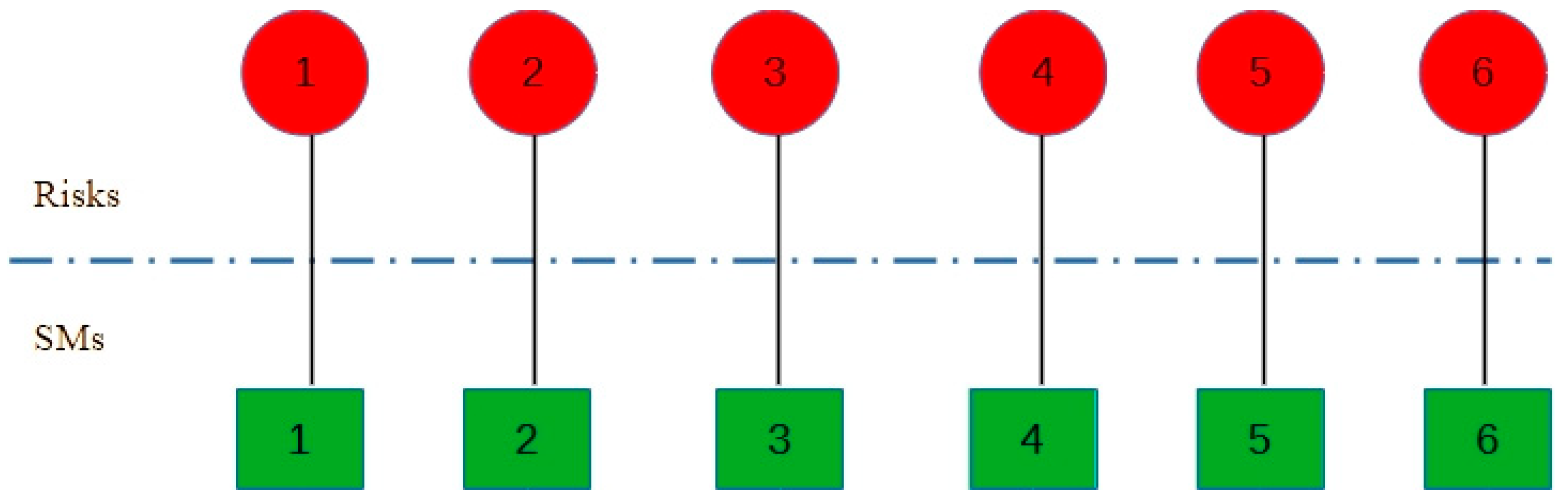
3.1. One-to-One Relationship Model

This model aims to take the most efficient safety measures in a given budget. To keep the model simpler and understandable, SMs are assumed to function independently without impacting other SMs. The main assumption of the model is that one SM can be taken for each risk and that each SM can affect one risk, as illustrated in Figure 3.

The assumptions of the model are as follows:

i.

Only one SM can be used for each risk;

ii.

Each SM can affect only one risk;

iii.

An SM cannot be partially applied (fully applied or not);

iv.

SMs do not pose an additional risk;

v.

Severity and likelihood levels, assessed by experts, are independent of each other;

vi.

Risks do not change during the review process;

vii.

The effects of the applied SMs on risks are stochastic;

viii.

If an SM is invested in, it will be implemented during the review period.

The 0/1 stochastic knapsack model is given in Equations (4)–(7):

Model notation

i: Risks (i = 1, 2, …, n);

q: SMs (q = 1, 2, …, m);

k: States (k = 1(improve), 2 (not changed) and 3 (worsen));

C_q: Cost of SM q;

B: Budget;

ρ_iqk: The probability value of transitioning to state k after implementing the qth SM for risk i;

L_iqk: The likelihood level of risk i in state k after the qth SM is implemented;

S_iqk: The severity level of risk i in state k after the qth SM is implemented;

ρ’_iqk: The probability value of transitioning to state k after not implementing any SM for risk i;

L’_iqk: The likelihood level of risk i in state k after not implementing any SM for risk i;

S’_iqk: The severity level of risk i in state k after not implementing any SM for risk i.

Decision Variable X_iq is defined in Equation (3):

$$X_{iq}:\left\{\begin{array}{l}1\mathrm{if}\mathrm{SM}q\mathrm{is}\mathrm{implemented}\mathrm{for}\mathrm{risk}i\\ 0\mathrm{otherwise}\hspace{1em}\hspace{1em}\hspace{1em}\hspace{1em}\end{array}\right.$$

(3)

Mathematical model

$$\mathrm{Min}Z=\sum _{i=1}^n\sum _{q\in M_i}{\mathrm{C}}_q\ast \times X_{\mathit{iq}}+\sum _{i=1}^n\sum _{q\in M_i}\left(\sum _{k=1}^2{\rho }_{\mathit{iqk}}\times L_{\mathit{iqk}}\times S_{\mathit{iqk}}\right)\times X_{\mathit{iq}}+\sum _{i=1}^n\sum _{q\in M_i}\left(\sum _{k=2}^3{{\rho }^{\prime }}_{\mathit{iqk}}\times {L^{\prime }}_{\mathit{iqk}}\times {S^{\prime }}_{\mathit{iqk}}\right)\times (1-X_{\mathit{iq}})$$

(4)

Subject to (s.t.)

$$\sum _{i=1}^n\sum _{q\in M_i}{C}_q\times X_{\mathit{iq}}\le B$$

(5)

$$\sum _{q\in M_i}{X}_{\mathit{iq}}\le 1\hspace{1em}\forall i$$

(6)

$$X_{\mathit{iq}}\in \left\{0,1\right\}\hspace{1em}\forall i,\forall q$$

(7)

Equation (4) aims to minimize the total cost, which includes the investment cost and the expected risks of implementing and not implementing SMs. Equation (5) ensures that the implementation cost does not exceed the budget. Equation (6) limits the maximum number of SMs that can be implemented for a risk to 1. Equation (7) defines the binary variables.

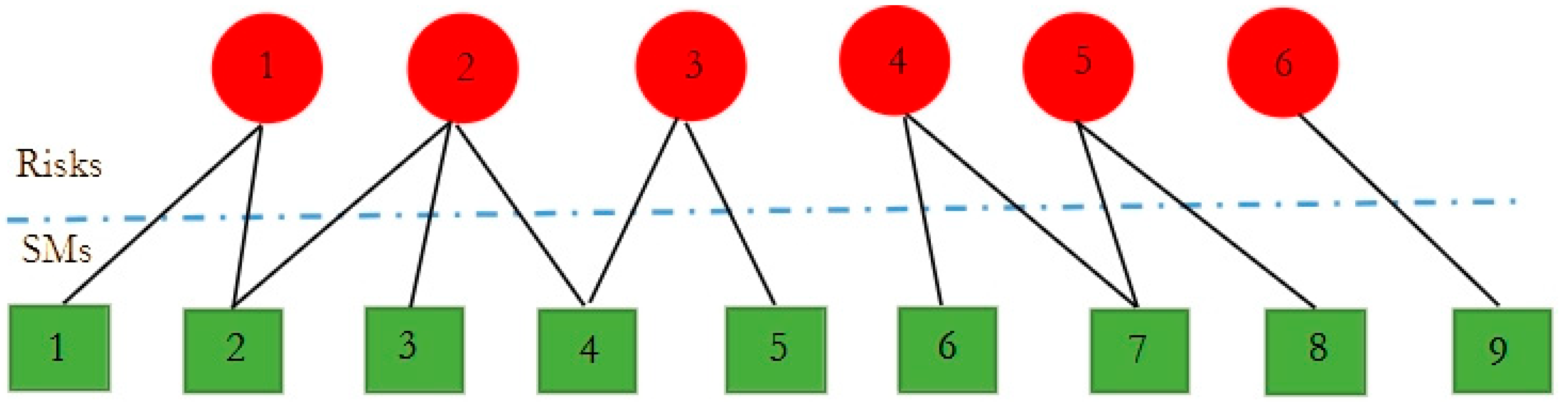
3.2. Multiple-Relationship Model

More than one SM impacting a risk can be identified during the risk assessment process, and the SMs that can be applied for these risks may affect a single risk or multiple risks simultaneously, as illustrated in Figure 4. For example, as seen in Figure 4, SMs 1 and 2 can be implemented together for risk 1. When implementing SM 2 for risk 1, it also affects risk 2. In such a case, there are several factors that complicate the assessment process. The first of these is that if a risk is affected by an SM bundle, the expected reduction in risk is considered to be a combination rather than the sum of the individual effects of the SMs. The second is whether there will be a change in risk as a result of the effects of SMs. To make the risk assessment process more effective, there is a need for approaches that take these challenges into account. Therefore, we extend the one-to-one relationship model and propose a new 0/1 stochastic knapsack model called the “Multiple-Relationship Model”.

The assumptions of the model are as follows:

i.

Several SMs can be taken for a risk;

ii.

An SM can affect more than one risk;

iii.

SMs cannot be partially applied (fully applied or not);

iv.

SMs do not pose an additional risk;

v.

The impacts of the SM bundles on risks are stochastic;

vi.

The probability (effects of SM bundles), severity, and likelihood values are dependent to SMs when implementing an SM bundle;

vii.

Risks do not change during the review process;

viii.

If an SM bundle is invested, it will be implemented during the review period.

Assumption vi posits that in the assessment of new probability, likelihood, and severity values of an SM bundle for a risk, the effects of individual SMs are not independent of each other. In other words, their combined impact should be evaluated rather than simply adding them together by using average expert predictions.

The 0/1 stochastic knapsack model is given in Equations (15)–(21).

Model notation

i: Risks (i = 1, 2, …, n).

q: SMs (q = 1, 2, …, m).

k: States (k = 1 (improve), 2 (not changed) and 3 (worsen)).

j: SM bundles (j = 1, 2, …, 2^m−1).

Q: A universal set of SM bundles given in Equation (8):

$$Q=\bigcup _{q=1}^m\left({\displaystyle \genfrac{}{}{0pt}{}{m}{q}}\right)$$

(8)

Max_num_i: The maximum number of SMs in bundle for risk i.

M_i: A set of j for risk i given in Equation (9):

$$M_i=\bigcup _{q=1}^{{\mathit{max}\_\mathit{num}}_i}\left({\displaystyle \genfrac{}{}{0pt}{}{m}{q}}\right),\subset Q$$

(9)

D_iq: A set of j including measure q for risk i and is given in Equation (10):

$$D_{\mathit{iq}}\subset M_i$$

(10)

W_ij: A parameter taking the values of 0 or 1 and defined by Equation (11):

$$W_{\mathit{ij}}:\left\{\begin{array}{l}1\hspace{1em}\mathrm{if}j\mathrm{is}\mathrm{element}\mathrm{of}{M}_i\\ 0\hspace{1em}\mathrm{otherwise}\end{array}\right.$$

(11)

C_q: Cost of SM q.

B: Budget.

ρ_ijk: The probability value of transitioning to state k after implementing the jth SM bundle for risk i.

L_ijk: The likelihood level of risk i in state k after the jth SM bundle is implemented.

S_ijk: The severity level of risk i in state k after the jth SM bundle is implemented.

ρ’_ik: The probability value of transitioning to state k after not implementing any SM bundle for risk i.

L’_ik: The likelihood value of risk i in state k after not implementing any SM bundle.

S’_ik: The severity value of risk i in state k after not implementing any SM bundle.

Decision Variables are given in Equations (12)–(14):

$$X_j:\left\{\begin{array}{l}1\mathrm{if}\mathrm{SM}\mathrm{bundle}j\mathrm{is}\mathrm{implemented}\\ 0\mathrm{otherwise}\hspace{1em}\hspace{1em}\hspace{1em}\hspace{1em}\hspace{1em}\end{array}\right.$$

(12)

$$Y_{\mathit{iq}}:\left\{\begin{array}{l}1\mathrm{if}\mathrm{SM}q\mathrm{is}\mathrm{implemented}\mathrm{for}\mathrm{risk}i\\ 0\mathrm{otherwise}\hspace{1em}\hspace{1em}\hspace{1em}\hspace{1em}\hspace{1em}\hspace{1em}\end{array}\right.$$

(13)

$$V_q:\left\{\begin{array}{l}1\mathrm{if}\mathrm{SM}q\mathrm{is}\mathrm{implemented}\\ 0\mathrm{otherwise}\hspace{1em}\hspace{1em}\hspace{1em}\hspace{1em}\hspace{1em}\end{array}\right.$$

(14)

Mathematical model

$$\mathrm{Min}Z=\sum _{q=1}^m{C}_q\times V_q+\sum _{i=1}^n\sum _{j\in M_i}\left(\sum _{k=1}^2{\rho }_{\mathit{ijk}}\times L_{\mathit{ijk}}\times S_{\mathit{ijk}}\right)\times W_{\mathit{ij}}\times X_j+\sum _{i=1}^n\sum _{k=2}^3(1-\sum _{j\in M_i}{W}_{\mathit{ij}}\times X_j)\times {{\rho }^{\prime }}_{\mathit{ik}}\times {L^{\prime }}_{\mathit{ik}}\times {S^{\prime }}_{\mathit{ik}}$$

(15)

s.t.

$$\sum _{q=1}^m{C}_q\times V_q\le B$$

(16)

$$\sum _{j\in M_i}{W}_{\mathit{ij}}\times X_j\le 1\hspace{1em}\forall i$$

(17)

$$\sum _{j\in D_{\mathit{iq}}}{X}_j=Y_{\mathit{iq}}\hspace{1em}\forall i,\forall q$$

(18)

$$n\times V_q-\sum _{i=1}^n{Y}_{\mathit{iq}}\ge 0\hspace{1em}\forall q\in D_{\mathit{iq}}$$

(19)

$$n\times V_q-\sum _{i=1}^n{Y}_{\mathit{iq}}\le n-1\hspace{1em}\forall q\in D_{\mathit{iq}}$$

(20)

$$Y_{\mathit{iq}},X_j,V_q\in \left\{0,1\right\}\hspace{1em}\forall i,\forall q,\forall j$$

(21)

Equation (15) aims to minimize the total cost, which includes the investment cost and the expected risks of implementing and not implementing SMs. Equation (16) ensures that the implementation cost does not exceed the budget. Equation (17) limits the number of SM bundles to 1, which can be implemented for a risk. Equation (18) defines whether an SM q is implemented or not for risk i. Equations (19) and (20) imply that if an SM bundle influencing more than one risk is implemented for any specific risk, it should similarly be applied to the other risks that it affects. Equation (21) defines the binary variables.

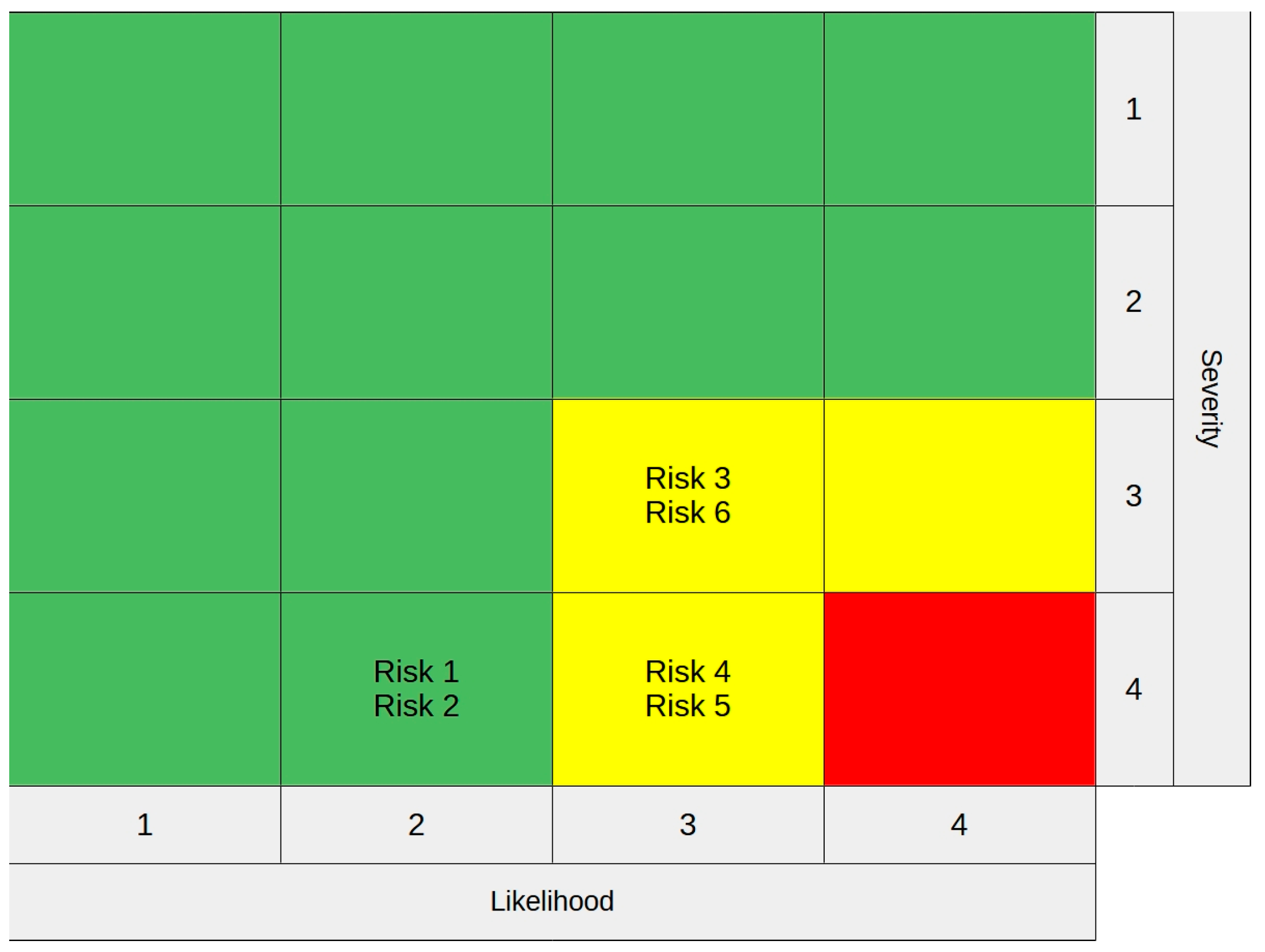
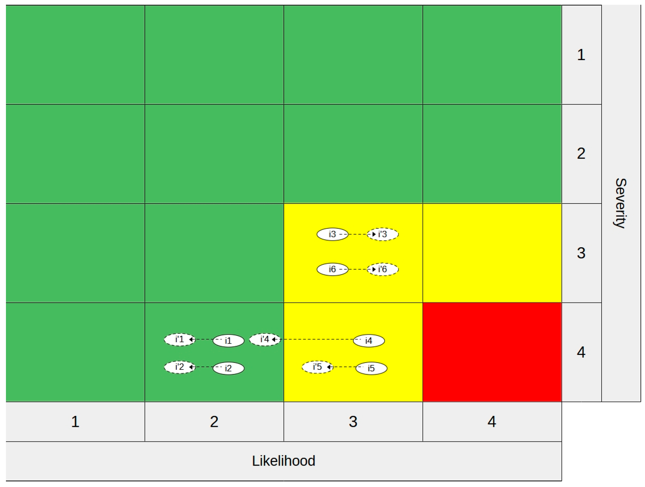
3.3. Multiple-Relationship Model Sample Problem

A real-world case study was carried out in the retail industry to demonstrate the proposed model’s sustainable value and practical applicability. Five experts made up the risk assessment team, which determined six critical operational risks (i = 1, 2…, 6) and assessed each one using the severity and likelihood scales shown in Table 2.

Table 3. Initial risk assessment.

i	Risks	Likelihood Score	Severity Score	Li	Si
1	Fire	2	4	0.0055	5,500,000
2	Electric shock	2	4	0.0055	5,500,000
3	Tripping over objects	3	3	0.055	550,000
4	Falling from a height	3	4	0.055	5,500,000
5	Falling materials from height	3	4	0.055	5,500,000
6	Manual lifting and transportation of heavy materials	3	3	0.055	550,000

shows the corresponding scores.

In Table 3, the last two columns (L_i and S_i) specify the likelihood and severity values, which are calculated by averaging the lower and upper bounds of associated levels shown in Table 2.

According to the risk assessment, two risks (1 and 2) are in the low category and four risks (3, 6 and 4, 5) are in the medium category, as presented in Figure 5. The risk assessment team identified nine potential SMs (q = 1, 2, …,9) that could be used for these risks on a USD 15,000 budget, which are given in

Table 4. The cost of SMs.

q	SM	Cq (USD)
1	Sprinkler system construction	20,000
2	Leakage current relay installation	500
3	Buying an insulation mat	1500
4	Maintenance of electrical installation	2500
5	Continuous monitoring to ensure there is no material left in the work area	13,000
6	Safety net stretching	10,000
7	Purchasing personal protective equipment	4000
8	Redesign of fallible materials to prevent falls	10,000
9	Purchasing a pallet truck	9000

along with their investment costs.

The number of SMs in each bundle per risk was limited by the parameter Max_num and determined to be three to control the complexity of judgment-based evaluations.

Table 5. SM bundles.

	Bundle j
M1	{1, 2, {1, 2}}
M2	{2, 3, 4, {2, 3}, {2, 4}, {3, 4}, {2, 3, 4}}
M3	{4, 5, {4, 5}}
M4	{6, 7, {6, 7}}
M5	{7, 8, {7, 8}}
M6	{9}

presents the feasible SM bundles that Mi generated under this constraint, and Figure 4 illustrates the relationships between risks and SMs.

These bundles served as a guide for defining the decision sets D_iq and impact parameters W_ij, as presented in

Table 6. D_iq sets.

Diq	Bundles Including SM q	Diq	Bundles Including SM q
i = 1, q = 1	{1, {1, 2}}	i = 3, q = 5	{5, {4, 5}}
i = 1, q = 2	{2, {1, 2}}	i = 4, q = 6	{6, {6, 7}}
i = 2, q = 2	{2, {2, 3}, {2, 4}, {2, 3, 4}}	i = 4, q = 7	{7, {6, 7}}
i = 2, q = 3	{3, {2, 3}, {3, 4}, {2, 3, 4}}	i = 5, q = 7	{7, {7, 8}}
i = 2, q = 4	{4, {2, 4}, {3, 4}, {2, 3, 4}}	i = 5, q = 8	{8, {7, 8}}
i = 3, q = 4	{4, {4, 5}}	i = 6, q = 9	{9}

and

Table 7. W_ij parameters.

i/j	1 (q1)	2 (q2)	3 (q3)	4 (q4)	5 (q5)	6 (q6)	7 (q7)	8 (q8)	9 (q9)	10 (q1–2)	11 (q2–3)	12 (q2–4)	13 (q3–4)	14 (q2–3–4)	15 (q4–5)	16 (q6–7)	17 (q7–8)
1	1	1	0	0	0	0	0	0	0	1	1	1	0	1	0	0	0
2	0	1	1	1	0	0	0	0	0	1	1	1	1	1	1	0	0
3	0	0	0	1	1	0	0	0	0	0	0	1	1	1	1	0	0
4	0	0	0	0	0	1	1	0	0	0	0	0	0	0	0	1	1
5	0	0	0	0	0	0	1	1	0	0	0	0	0	0	0	1	1
6	0	0	0	0	0	0	0	0	1	0	0	0	0	0	0	0	0

, respectively.

The remaining parameters, namely the costs of SM bundles (C_q), the impact probability values (ρ_ijk), the likelihood levels (L_ijk), and the severity levels (S_ijk) after implementing SMs, are presented in

Table 8. Costs of SM bundles.

j	1 (q1)	2 (q2)	3 (q3)	4 (q4)	5 (q5)	6 (q6)	7 (q7)	8 (q8)	9 (q9)	10 (q1–2)	11 (q2–3)	12 (q2–4)	13 (q3–4)	14 (q2–3–4)	15 (q4–5)	16 (q6–7)	17 (q7–8)
Cj ($)	20,000	500	1500	2500	13,000	10,000	4000	10,000	9000	20,500	2000	3000	4000	4500	15,500	14,000	14,000

,

Table 9. The impact probability values when implementing SM bundles (ρ_ijk).

i/j	k	1 (q1)	2 (q2)	3 (q3)	4 (q4)	5 (q5)	6 (q6)	7 (q7)	8 (q8)	9 (q9)	10 (q1–2)	11 (q2–3)	12 (q2–4)	13 (q3–4)	14 (q2–3–4)	15 (q4–5)	16 (q6–7)	17 (q7–8)
1	1	0.83	0.66	0	0	0	0	0	0	0	0.94	0.66	0.66	0	0.66	0	0	0
	2	0.17	0.34	0	0	0	0	0	0	0	0.06	0.34	0.34	0	0.34	0	0	0
2	1	0	0.66	0.65	0.61	0	0	0	0	0	0.66	0.87	0.85	0.83	0.966	0.61	0	0
	2	0	0.34	0.35	0.39	0	0	0	0	0	0.34	0.13	0.15	0.17	0.034	0.39	0	0
3	1	0	0	0	0.61	0.72	0	0	0	0	0	0	0.61	0.61	0.61	0.92	0	0
	2	0	0	0	0.39	0.28	0	0	0	0	0	0	0.39	0.39	0.39	0.08	0	0
4	1	0	0	0	0	0	0.72	0.57	0	0	0	0	0	0	0	0	0.93	0.57
	2	0	0	0	0	0	0.28	0.43	0	0	0	0	0	0	0	0	0.07	0.43
5	1	0	0	0	0	0	0	0.57	0.58	0	0	0	0	0	0	0	0.57	0.91
	2	0	0	0	0	0	0	0.43	0.42	0	0	0	0	0	0	0	0.43	0.09
6	1	0	0	0	0	0	0	0	0	0.78	0	0	0	0	0	0	0	0
	2	0	0	0	0	0	0	0	0	0.22	0	0	0	0	0	0	0	0

,

Table 10. The likelihood values when implementing SM bundles (L_ijk).

i/j	k	1 (q1)	2 (q2)	3 (q3)	4 (q4)	5 (q5)	6 (q6)	7 (q7)	8 (q8)	9 (q9)	10 (q1–2)	11 (q2–3)	12 (q2–4)	13 (q3–4)	14 (q2–3–4)	15 (q4–5)	16 (q6–7)	17 (q7–8)
1	1	0.0005	0.0005	0	0	0	0	0	0	0	0.0005	0.0005	0.0005	0	0.0005	0	0	0
	2	0.005	0.005	0	0	0	0	0	0	0	0.005	0.005	0.005	0	0.005	0	0	0
2	1	0	0.0005	0.0005	0.0005	0	0	0	0	0	0.0005	0.0005	0.0005	0.0005	0.0005	0.0005	0	0
	2	0	0.005	0.005	0.005	0	0	0	0	0	0.005	0.005	0.005	0.005	0.005	0.005	0	0
3	1	0	0	0	0.0055	0.0055	0	0	0	0	0	0	0.0055	0.0055	0.0055	0.0055	0	0
	2	0	0	0	0.055	0.055	0	0	0	0	0	0	0.055	0.055	0.055	0.055	0	0
4	1	0	0	0	0	0	0.0055	0.0055	0	0	0	0	0	0	0	0	0.0055	0.0055
	2	0	0	0	0	0	0.055	0.055	0	0	0	0	0	0	0	0	0.055	0.055
5	1	0	0	0	0	0	0	0.0055	0.0055	0	0	0	0	0	0	0	0.0055	0.0055
	2	0	0	0	0	0	0	0.055	0.055	0	0	0	0	0	0	0	0.055	0.055
6	1	0	0	0	0	0	0	0	0	0.0055	0	0	0	0	0	0	0	0
	2	0	0	0	0	0	0	0	0	0.055	0	0	0	0	0	0	0	0

and

Table 11. The severity values in a thousand terms when implementing SM bundles (S_ijk).

i/j	k	1 (q1)	2 (q2)	3 (q3)	4 (q4)	5 (q5)	6 (q6)	7 (q7)	8 (q8)	9 (q9)	10 (q1–2)	11 (q2–3)	12 (q2–4)	13 (q3–4)	14 (q2–3–4)	15 (q4–5)	16 (q6–7)	17 (q7–8)
1	1	5500	5500	0	0	0	0	0	0	0	5500	5500	5500	0	5500	0	0	0
	2	5500	5500	0	0	0	0	0	0	0	5500	5500	5500	0	5500	0	0	0
2	1	0	5500	5500	5500	0	0	0	0	0	5500	5500	5500	5500	5500	5500	0	0
	2	0	5500	5500	5500	0	0	0	0	0	5500	5500	5500	5500	5500	5500	0	0
3	1	0	0	0	550	550	0	0	0	0	0	0	550	550	550	550	0	0
	2	0	0	0	550	550	0	0	0	0	0	0	550	550	550	550	0	0
4	1	0	0	0	0	0	5500	5500	0	0	0	0	0	0	0	0	5500	5500
	2	0	0	0	0	0	5500	5500	0	0	0	0	0	0	0	0	5500	5500
5	1	0	0	0	0	0	0	5500	5500	0	0	0	0	0	0	0	5500	5500
	2	0	0	0	0	0	0	5500	5500	0	0	0	0	0	0	0	5500	5500
6	1	0	0	0	0	0	0	0	0	550	0	0	0	0	0	0	0	0
	2	0	0	0	0	0	0	0	0	550	0	0	0	0	0	0	0	0

, and the impact probability values, the likelihood, and the severity levels after not implementing SMS (ρ’_ik and L’_ik and S’_ik) are shown in

Table 12. The impact probability (ρ’_ik), likelihood (L’_ik), and severity (S’_ik) values when not implementing SM bundles.

i	k	ρ’ik	L’ik	S’ik
1	2	0.98	0.0055	5,500,000
	3	0.02	0.055	5,500,000
2	2	0.98	0.0055	5,500,000
	3	0.02	0.055	5,500,000
3	2	0.97	0.055	550,000
	3	0.03	0.55	550,000
4	2	0.95	0.055	5,500,000
	3	0.05	0.55	5,500,000
5	2	0.96	0.055	5,500,000
	3	0.04	0.55	5,500,000
6	2	0.97	0.055	550,000
	3	0.03	0.55	550,000

.

Additionally, according to assumption vi, the model does not treat the impacts of SM bundles additively, allowing for non-linear effects among SMs. For example, Table 9 shows that the individual impact probabilities for SM 1 and SM 2 on risk 1 are 0.83 and 0.66, respectively. Instead of using arithmetic summation, their combined impact as a bundle (q_1–2) is found to be 0.94, which reflects an expert group consensus. This structure makes it possible for the model to more accurately depict the overlapping effects of SMs.

Solution for the Sample Problem and Implications

The sample problem was solved global optimally using a standard personal computer equipped with a 1.6 Ghz processor and 8 Gigabyte of RAM by using CPLEX solver (version 48.6.0) GAM optimization software, demonstrating that the proposed approach is computationally feasible using modest hardware configurations. The optimal solution is given in

Table 13. The optimal solution for the multiple-relationship model sample problem.

X(j)	Value	Y (i, q)	Value	V(q)	Value
j = 1	0	i1, q1	0	q1	0
j = 2	1	i1, q2	1	q2	1
j = 3	0	i2, q2	1	q3	0
j = 4	0	i2, q3	0	q4	0
j = 5	0	i2, q4	0	q5	0
j = 6	0	i3, q4	0	q6	1
j = 7	0	i3, q5	0	q7	1
j = 8	0	i4, q6	1	q8	0
j = 9	0	i4, q7	1	q9	0
j = 10	0	i5, q7	1
j = 11	0	i5, q8	0
j = 12	0	i6, q9	0
j = 13	0
j = 14	0
j = 15	0
j = 16	1
j = 17	0

. In the optimal solution, two SM bundles (X (2) and X (16)) were selected for investment: these included investments in SM 2, SM 6, and SM 7, which together addressed risks 1, 2, 4, and 5. With a USD 14,500 total investment, the objective function value was USD 312,523, with an overall expected risk reduction of USD 427,977.

Investing in SM 2, which costs USD 500, impacted risks 1 and 2, resulting in a USD 35,937 risk reduction, while in SMs 6–7, which cost USD 14,000, and impacted risks 4 and 5, resulting in a significant USD 408,374 risk reduction. Risks 3 and 6 did not receive investment because of financial limitations, with risk expected to increase by USD 8167.5 apiece. A method that promotes economical and risk-aware sustainable planning is highlighted by the model’s optimization logic, which gives priority to SMs with high benefit-to-cost ratios and alignment with feasibility constraints. The model maximizes impact per unit cost by strategically allocating limited resources towards the most important and reducible risks. Here, priority was given to risks 4 and 5, which had the highest initial risk levels.

Figure 6 illustrates the changes in the risk profile resulting from implementing SMs. Following implementation, there were significant expected risk reductions for risks 1, 2, 4, and 5. Since risks 3 and 6 were not covered by the selected bundles, the expected risks for these risks increased. Additionally, risk 4 changed from medium to low risk on the matrix, indicating that the model can improve safety performance under certain conditions. This result highlights how the suggested model adheres to the sustainable risk governance principles of maximizing resource utilization, integrating expert judgment, and enhancing resilience while staying within budgetary limits.

The case study demonstrates how the suggested model aligns effective risk mitigation with sustainability principles, thereby supporting multiple SDGs. It promotes the responsible and efficient use of limited safety resources (SDGs 8 and 12) and improves OHS (SDG 3). It supports data-driven decision-making, leading to more innovative and resilient safety planning (SDG 9). Its ability to adapt to environmental risks makes it relevant to efforts to build climate resilience (SDG 13). The model’s applicability in promoting resilient and sustainable development is demonstrated by its scalability across various sectors and levels of governance.

4. Limitations and Challenges of the Proposed Models

The initial step in implementing the suggested approach is to determine the likelihood and severity of risks, as well as the associated costs and impact probabilities of SMs. The accuracy of the models depends on the availability of reliable data for risk assessment and SM impact probabilities. Expert judgment may be required when data are scarce, introducing subjectivity and uncertainty. Data collection can become resource-intensive and time-consuming, and the collected data may also be prone to bias and uncertainty.

The risk matrix method is straightforward and user-friendly. However, its simplicity comes with the uncertainty and subjectivity of inputs and outputs, which can significantly impact the optimization outcomes and lead to a locally optimal or non-optimal set of SMs. The risk levels allocated to each cell of a risk matrix may not be equivalent due to subjective assessments and the discretization of risk levels. Conversely, our study presumes that each cell of the risk matrix holds the same quantitative value for the level of risk.

Furthermore, the multiple-relationship model can become computationally complex for large problems due to the combinatorial nature of SM bundles and total risks for high-risk industries. Decision-makers must balance computational feasibility with model accuracy, potentially requiring heuristics or simplification methods for larger datasets. To overcome computational complexity, decision-makers might use the following solution algorithm:

Step 1: Identify risks.

Step 2: Run the proposed model.

Step 3: (a) If the model produces a solution, go to Step 6; (b) if the model does not produce a solution, proceed to Step 4.

Step 4: Evaluate whether simplification is possible by excluding low-priority risks and by limiting the maximum number of SMs per risk, as proposed in this study. In particular, the maximum bundle size of three (max_num_i = 3) proposed in this study provides a natural answer for reducing the complexity of SM impact modeling. Firstly, a graphical multiple-relationship model, as shown in Figure 4, can be developed. Then, for each risk, the risk assessment team can select one, two, or three effective SMs and eliminate the rest.

(a) If simplification is possible, then go back to Step 2.

(b) If not, proceed to Step 5.

Step 5: Develop a metaheuristic algorithm, then proceed to Step 6.

Step 6: Evaluate the solution.

Metaheuristics are known for their speed but may not guarantee a global optimum. However, developing such an algorithm falls outside the scope of this study.

Bias and uncertainty from expert judgment elicitation can be mitigated through structured expert elicitation techniques, gathering multiple opinions, and providing training to experts on the elicitation process. Proper calibration methods can also help to improve the reliability of expert-driven probability estimates.

The proposed multiple-relationship model, which addresses the complex frameworks of interdependent SMs and their combined impact on numerous risks, is, as far as we know, a novel approach in the field. Therefore, no existing model is readily available that the proposed model can be compared against. For comparison purposes, however, a traditional deterministic benchmark model can be constructed by simplifying the proposed model. The deterministic model uses a pessimistic strategy recently proposed by Eslami Baladeh [86], and it can be considered the closest alternative to the proposed model in the literature. This model acknowledges the fact that a single SM may have impact multiple risks; however, it implements only one SM for each risk in the following fashion: the updated risk level that results from applying multiple SMs to a particular risk is estimated by calculating the minimum of the updated risk levels that would be produced by applying each SM independently. Moreover, the impact probabilities are eliminated to convert the stochastic model to a deterministic model. The impact probability of implementing an SM leading to an improvement and a decrease in risk level (ρ_ij1) is equal to 1, as the impact probability of not implementing an SM and the resulting risk level remaining unchanged (ρ’_i2) is also equal to 1.

We use the same numerical example employed in the previous section: six risks, nine candidate SMs, and a USD 15,000 budget. The SM–risk relationship in the deterministic benchmark model is also as illustrated in Figure 4. In this case, for example, risk 1 can be impacted by either SM 1 or SM 2 but not both as a bundle. However, SM 2 can impact both risks 1 and 2 simultaneously.

The results related to the selected metrics of the comparative analysis are illustrated in

Table 14. Comparative analysis results for proposed and deterministic models.

Metric	Deterministic Model	Proposed Stochastic Model
Objective Function Value	385,575	312,523
Total Expected Risk Reduction	353,925	427,977
Total Budget Utilized	13,500	14,500
Expected Risk Reduction per USD 1	26.2	29.5
Value of Stochastic Solution (VSS)	–	73,052
Solution Time (seconds)	0.39	0.11
Invested SMs	q2, q7, q9	q2, q6–7
Impacted Risks	i1, i2, i4, i5, i6	i1, i2, i4, i5

.

The findings demonstrate the effectiveness of incorporating stochasticity into SM impact modeling. The proposed model achieved a 18.9% reduction in the objective function value compared to the deterministic model, along with a higher expected total risk reduction (427,977 vs. 353,925). The Value of the Stochastic Solution (VSS), calculated as 73,052, confirmed the practical advantage of explicitly accounting for uncertainty. While the deterministic model had a slightly faster solution time (0.09 vs. 0.11 s), this marginal difference was outweighed by the performance gains of the stochastic approach.

Additionally, the stochastic model demonstrated a more efficient use of resources. Although it utilized slightly more of the budget (USD 14,500 vs. USD 13,500), it yielded a significantly higher expected risk reduction. Regarding the efficiency of the models, the average risk reduction per dollar spent was calculated to be 29.5 for the stochastic model and 26.2 for the deterministic model. This finding underscores the notion that the stochastic model not only improves the total outcomes but also delivers more value per unit of investment. The findings of this study serve to reinforce the importance of modeling uncertainty and risk interdependencies, particularly in circumstances where resources are limited, utilized responsibly, and in need of optimization.

These findings are consistent with the risk-based approach advocated in the OHS management systems standards [101], which promote proactive hazard identification and SM selection based on informed, quantitative prioritization. The model’s integration of stochasticity and interdependencies of SMs into the decision-making process is a significant contribution to sustainable OHS outcomes, aligning with SDGs 3 and 8. Additionally, the proposed models contribute to advancing SDG 12, which calls for promoting resource-efficient interventions that maximize safety impacts.

Furthermore, the models reflect technological and operational innovation in safety planning, thus supporting SDG 9 by assisting industries with optimizing risk control decisions and enhancing infrastructure resilience. Although the model was developed for managing occupational risks, it is nevertheless adaptable for use in climate risk reduction and disaster resilience planning. This adaptability extends to allocating limited resources with a view to mitigating flood, heat, or wildfire risks. The cross-domain applicability of the models enhances their contribution to SDG 13 by supporting evidence-based, uncertainty-aware decisions that strengthen adaptive capacity for climate-related hazards. Consequently, the proposed methodology enhances not only the technical precision of safety management but also its contribution to SDGs and occupational safety frameworks.

Moreover, the practical implementation of the proposed models may be impeded by structural limitations in many sectors. Despite ongoing global efforts to address this issue, sectors dominated by dangerous and informal employment along with small- and medium-sized enterprises (SMEs) continue to face high safety risks and poor working conditions. As emphasized by the International Labour Organization, the economic and social burdens of occupational injuries and illnesses in these sectors are frequently externalized onto workers and their families, complicated by underdeveloped compensation systems and chronic underinvestment in SMs [102]. These systemic challenges may impede the adoption of the proposed models, particularly in contexts where institutional capacity, enforcement mechanisms, or incentives for proactive safety investments are inadequate.

To maintain simplicity in this matter and concentrate on the methodology, the models rely on certain assumptions, such as the maximum number of SMs in a bundle for the multiple-relationship model and the quantifiability of benefits gained from implementing SMs. These assumptions generally apply to many situations; however, they may not hold depending on the specific application.

Knapsack problems have emerged as a fundamental and extensively studied domain within combinatorial optimization since their popularization by Martello and Toth [103]. There are many variants of knapsack problems, which are generally NP-hard. However, single knapsack problems, as used in the proposed models, are classified as NP-hard in the weak sense. This classification implies that they can be solved in pseudo-polynomial time using dynamic programming [104]. Consequently, the proposed model can be solved to determine global optimality using optimization software for various real-life applications in the risk assessment process. However, if the model is extended by increasing the number of risks or SM bundles or reformulated as a multi-objective or multi-dimensional knapsack problem [105], a metaheuristic algorithm will be necessary to solve it.

5. Conclusions

Ensuring workplace safety is crucial, as failures in risk management can result in fatalities and financial losses. This study introduces two novel stochastic knapsack models that integrate expert-elicited probabilities with independent and interdependent SMs to optimize safety investments under budget constraints. The proposed models enhance traditional risk management techniques by addressing the stochastic nature of SMs, moving beyond the limitations of deterministic approaches.

By incorporating stochastic impacts and interdependencies among SMs, the models provide a flexible and realistic approach to risk optimization. According to the comparative analysis, the proposed model performs better than the deterministic one in a number of important areas. With an expected risk reduction per dollar of 29.5 as opposed to 26.2, it specifically demonstrates a higher overall efficiency and achieves an 18.9% reduction in residual risk. The value of explicitly modeling uncertainty is further supported by the VSS, which is determined to be 73,052.

Despite these benefits, there are a number of restrictions on the model’s applicability. Its computational complexity may increase dramatically in large-scale scenarios, and its use depends on expert judgment, which can introduce bias and variability. However, bias and variability could be lessened and scalability improved by using structured expert elicitation techniques or integrating machine learning or Bayesian network techniques. To overcome computational complexity, decision-makers might use metaheuristics in addition to simplifying the assumptions proposed in this study to solve more complex versions of the proposed model.

Furthermore, structural barriers to practical implementation may arise in industries with inadequate institutional capacity or chronic underinvestment in safety, especially in SMEs. The model’s adoption and practical utility can be improved by addressing these issues through capacity-building programs, incentive-based policy interventions, and including simplified, scalable decision-support tools designed for resource-constrained environments.

Additionally, the model’s emphasis on resource-efficient, uncertainty-aware SM selection promotes long-term occupational safety results. This is particularly important for its adherence to international frameworks, including the SDGs and ISO 45001’s [101] risk-based thinking approach. By promoting proactive, data-driven safety planning, the model aligns with the SDGs 3 and 8. By emphasizing the optimization of limited resources, it also contributes to SDG 12. Additionally, by encouraging evidence-based innovation in risk management systems, the model supports SDG 9. Its relevance for SDG 13 is enhanced by its adaptability to climate risk contexts, providing a strong framework for managing flood, heat, or wildfire risks with limited public resources.

The proposed models provide useful guidance for national safety regulators, regional authorities, and international organizations looking for ways to optimize the allocation of limited safety resources. Its potential as a flexible decision-support tool is highlighted by its adaptability across industries and risk categories, including environmental, occupational, and climate-related hazards. Its alignment with the SDGs is improved by this flexibility. Thus, the model promotes policy frameworks that seek inclusive, safe, and sustainable development outcomes in addition to advancing safety management practices.

Future research should explore extending the model to multi-period risk assessment, integrating machine learning for probability estimation, and improving computational scalability for larger datasets. Additionally, incorporating behavioral factors and organizational dynamics could further refine the decision-making framework. Furthermore, exploring real-world applications of this model in high-risk industries will facilitate the validation of its impact on sustainability. Moreover, the model’s contribution to efforts to promote sustainable development may be strengthened by expanding it to cover multi-objective or climate-related frameworks.

In conclusion, the proposed stochastic knapsack model represents a significant advancement in OHS risk management. By leveraging expert-elicited probabilities and interdependent risk mitigation strategies, it offers a structured and adaptable framework for optimizing safety investments. It offers a reproducible, resource-efficient methodology that allows organizations to make better informed, equitable, and sustainable OHS decisions.

References

1. Baybutt, P. Designing Risk Matrices to Avoid Risk Ranking Reversal Errors. Process. Saf. Prog. 2016, 35, 41–46. [Google Scholar] [CrossRef]
2. Coppola, D.P. Chapter 3—Risk and Vulnerability. In Introduction to International Disaster Management, 4th ed.; Coppola, D.P., Ed.; Butterworth-Heinemann: Oxford, UK, 2020; pp. 177–265. ISBN 978-0-12-817368-8. [Google Scholar]
3. Mentges, A.; Halekotte, L.; Schneider, M.; Demmer, T.; Lichte, D. A Resilience Glossary Shaped by Context: Reviewing Resilience-Related Terms for Critical Infrastructures. Int. J. Disaster Risk Reduct. 2023, 96, 103893. [Google Scholar] [CrossRef]
4. Mohamed, A.-M.O.; Paleologos, E.K.; Howari, F.M. Pollution Assessment for Sustainable Practices in Applied Sciences and Engineering; Butterworth-Heinemann: Oxford, UK, 2021; ISBN 978-0-12-809582-9. [Google Scholar]
5. Bao, C.; Li, J.; Wu, D. A Fuzzy Mapping Framework for Risk Aggregation Based on Risk Matrices. J. Risk Res. 2018, 21, 539–561. [Google Scholar] [CrossRef]
6. Dai, Y.; Tong, X.; Wang, L. Workplace Safety Accident, Employee Treatment, and Firm Value: Evidence from China. Econ. Model. 2022, 115, 105960. [Google Scholar] [CrossRef]
7. Li, J.; Bao, C.; Wu, D. How to Design Rating Schemes of Risk Matrices: A Sequential Updating Approach. Risk Anal. 2018, 38, 99–117. [Google Scholar] [CrossRef]
8. Xu, H.; Mei, Q.; Liu, S.; Zhang, J.; Khan, M.A.S. Understand, Track and Develop Enterprise Workplace Safety, and Sustainability in the Industrial Park. Heliyon 2023, 9, e16717. [Google Scholar] [CrossRef]
9. Elmonstri, M. Review of the Strengths and Weaknesses of Risk Matrices. J. Risk Anal. Crisis Response 2014, 4, 49–57. [Google Scholar] [CrossRef]
10. Nguembi, I.P.; Yang, L.; Appiah, V.S. Safety and Risk Management of Chinese Enterprises in Gabon’s Mining Industry. Heliyon 2023, 9, e20721. [Google Scholar] [CrossRef]
11. UN General Assembly. Transforming Our World: The 2030 Agenda for Sustainable Development, A/RES/70/1; United Nations Department of Economic and Social Affairs: New York, NY, USA, 2015. [Google Scholar]
12. Mazzi, A. Environmental and Safety Risk Assessment for Sustainable Circular Production: Case Study in Plastic Processing for Fashion Products. Heliyon 2023, 9, e21352. [Google Scholar] [CrossRef]
13. Varadharajan, S.; Bajpai, S. Chronicles of Security Risk Assessment in Process Industries: Past, Present and Future Perspectives. J. Loss Prev. Process Ind. 2023, 84, 105096. [Google Scholar] [CrossRef]
14. ISO 31000:2018; Risk Management—Guidelines. International Organization for Standardization: Geneva, Switzerland, 2018.
15. PMI. The Standard for Risk Management in Portfolios, Programs, and Projects; PMI: Newtown Square, PA, USA, 2019. [Google Scholar]
16. Albanesi, B.; Godono, A.; Plebani, F.; Mustillo, G.; Fumagalli, R.; Clari, M. Exploring Strategies and Tools to Prevent Accidents or Incidents in Atypical Scenarios. A Scoping Review. Saf. Sci. 2023, 163, 106124. [Google Scholar] [CrossRef]
17. Choo, B.L.; Go, Y.I. Energy Storage for Large Scale/Utility Renewable Energy System—An Enhanced Safety Model and Risk Assessment. Renew. Energy Focus 2022, 42, 79–96. [Google Scholar] [CrossRef]
18. Langdalen, H.; Abrahamsen, E.B.; Abrahamsen, H.B. A New Framework to Idenitfy and Assess Hidden Assumptions in the Background Knowledge of a Risk Assessment. Reliab. Eng. Syst. Saf. 2020, 200, 106909. [Google Scholar] [CrossRef]
19. Chen, C.; Reniers, G.; Khakzad, N.; Yang, M. Operational Safety Economics: Foundations, Current Approaches and Paths for Future Research. Saf. Sci. 2021, 141, 105326. [Google Scholar] [CrossRef]
20. Levine, E.S. Improving Risk Matrices: The Advantages of Logarithmically Scaled Axes. J. Risk Res. 2012, 15, 209–222. [Google Scholar] [CrossRef]
21. Manuele, F.A. Advanced Safety Management Focusing on Z10 and Serious Injury Prevention, 2nd ed.; Wiley: Hoboken, NJ, USA, 2014; ISBN 978-1-118-84098-6. [Google Scholar]
22. Marhavilas, P.K.; Koulouriotis, D.E. A Risk-Estimation Methodological Framework Using Quantitative Assessment Techniques and Real Accidents’ Data: Application in an Aluminum Extrusion Industry. J. Loss Prev. Process. Ind. 2008, 21, 596–603. [Google Scholar] [CrossRef]
23. Altenbach, T.J. Comparison of Risk Assessment Techniques from Qualitative to Quantitative. In Proceedings of the American Society of Mechanical Engineers, Pressure Vessels and Piping Division, Hono lulu, HI, USA, 23–27 July 1995; Volume 296. [Google Scholar]
24. Duijm, N.J. Recommendations on the Use and Design of Risk Matrices. Saf. Sci. 2015, 76, 21–31. [Google Scholar] [CrossRef]
25. Wanner, P.; Freis, M.; Peternell, M.; Kelm, V. Risk Classification of Contaminated Sites—Comparison of the Swedish and the German Method. J. Environ. Manag. 2023, 327, 116825. [Google Scholar] [CrossRef]
26. Wilkinson, G.; David, R. Back to Basics: Risk Matrices and ALARP. In Safety-Critical Systems: Problems, Process and Practice, Proceedings of the 17th Safety-Critical Systems Symposium, SSS 2009, Brighton, UK, 3–5 February 2009; Springer: London, UK, 2009. [Google Scholar]
27. Xu, Y.; Reniers, G.; Yang, M.; Yuan, S.; Chen, C. Uncertainties and Their Treatment in the Quantitative Risk Assessment of Domino Effects: Classification and Review. Process. Saf. Environ. Prot. 2023, 172, 971–985. [Google Scholar] [CrossRef]
28. Baybutt, P. Guidelines for Designing Risk Matrices. Process. Saf. Prog. 2018, 37, 49–55. [Google Scholar] [CrossRef]
29. Ball, D.J.; Watt, J. Further Thoughts on the Utility of Risk Matrices. Risk Anal. 2013, 33, 2068–2078. [Google Scholar] [CrossRef]
30. Wall, K.D. The Trouble with Risk Matrices; Naval Postgraduate School (DRMI): Monterey, CA, USA, 2011; p. 26. [Google Scholar]
31. Markowski, A.S.; Mannan, M.S. Fuzzy Risk Matrix. J. Hazard. Mater. 2008, 159, 152–157. [Google Scholar] [CrossRef] [PubMed]
32. Marhavilas, P.K.; Filippidis, M.; Koulinas, G.K.; Koulouriotis, D.E. The Integration of HAZOP Study with Risk-Matrix and the Analytical-Hierarchy Process for Identifying Critical Control-Points and Prioritizing Risks in Industry—A Case Study. J. Loss Prev. Process Ind. 2019, 62, 103981. [Google Scholar] [CrossRef]
33. Cheng, Y.-C.; Liao, S.-W.; Alauddin, M.; Amyotte, P.; Shu, C.-M. Redefining of Potential Dust Explosion Risk Parameters for Additives in the Petrochemical Manufacturing Process. Process. Saf. Environ. Prot. 2023, 169, 472–480. [Google Scholar] [CrossRef]
34. Comberti, L.; Demichela, M. Customised Risk Assessment in Manufacturing: A Step towards the Future of Occupational Safety Management. Saf. Sci. 2022, 154, 105809. [Google Scholar] [CrossRef]
35. Seker, S. A Model for Risk Assessment in Glass Manufacturing Using Risk Matrix Technique and IVIF-TOPSIS Method. J. Intell. Fuzzy Syst. 2021, 42, 541–550. [Google Scholar] [CrossRef]
36. Du, M.; Zhang, S.M.; Shang, W.J.; Yan, W.X.; Liu, Q.; Qin, C.Y.; Liu, M.; Liu, J. 2022 Multiple-Country Monkeypox Outbreak and Its Importation Risk into China: An Assessment Based on the Risk Matrix Method. Biomed. Env. Sci. 2022, 35, 878–887. [Google Scholar]
37. Lohmann, D.; Lang-Welzenbach, M.; Feldberger, L.; Sommer, E.; Bücken, S.; Lotter, M.; Ott, O.J.; Fietkau, R.; Bert, C. Risk Analysis for Radiotherapy at the Universitätsklinikum Erlangen. Z. Für Med. Phys. 2022, 32, 273–282. [Google Scholar] [CrossRef]
38. Mbah, L.T.; Molua, E.L.; Bomdzele, E.; Egwu, B.M.J. Farmers’ Response to Maize Production Risks in Cameroon: An Application of the Criticality Risk Matrix Model. Heliyon 2023, 9, e15124. [Google Scholar] [CrossRef]
39. Durdyev, S.; Mohandes, S.R.; Tokbolat, S.; Sadeghi, H.; Zayed, T. Examining the OHS of Green Building Construction Projects: A Hybrid Fuzzy-Based Approach. J. Clean. Prod. 2022, 338, 130590. [Google Scholar] [CrossRef]
40. Spasenic, Z.; Makajic-Nikolic, D.; Benkovic, S. Integrated FTA-Risk Matrix Model for Risk Analysis of a Mini Hydropower Plant’s Project Finance. Energy Sustain. Dev. 2022, 70, 511–523. [Google Scholar] [CrossRef]
41. Tian, Z.; Chen, Q.; Zhang, T. A Method for Assessing the Crossed Risk of Construction Safety. Saf. Sci. 2022, 146, 105531. [Google Scholar] [CrossRef]
42. Bolbot, V.; Theotokatos, G.; McCloskey, J.; Vassalos, D.; Boulougouris, E.; Twomey, B. A Methodology to Define Risk Matrices—Application to Inland Water Ways Autonomous Ships. Int. J. Nav. Archit. Ocean. Eng. 2022, 14, 100457. [Google Scholar] [CrossRef]
43. Georgiev, K. Aviation Safety Training Methodology. Heliyon 2021, 7, e08511. [Google Scholar] [CrossRef]
44. Ebrahimi, H.; Sattari, F.; Lefsrud, L.; Macciotta, R. Human Vulnerability Modeling and Risk Analysis of Railway Transportation of Hazardous Materials. J. Loss Prev. Process. Ind. 2022, 80, 104882. [Google Scholar] [CrossRef]
45. Sun, S.; Gao, G.; Li, Y.; Zhou, X.; Huang, D.; Chen, D.; Li, Y. A Comprehensive Risk Assessment of Chinese High-Speed Railways Affected by Multiple Meteorological Hazards. Weather. Clim. Extrem. 2022, 38, 100519. [Google Scholar] [CrossRef]
46. Firoozzare, A.; Ghazanfari, S.; Yousefian, N. Designing and Analyzing the Motivational Risk Profile of Healthy Food and Agricultural Products Purchase. J. Clean. Prod. 2023, 432, 139693. [Google Scholar] [CrossRef]
47. Domínguez, C.R.; Martínez, I.V.; Piñón Peña, P.M.; Rodríguez Ochoa, A. Analysis and Evaluation of Risks in Underground Mining Using the Decision Matrix Risk-Assessment (DMRA) Technique, in Guanajuato, Mexico. J. Sustain. Min. 2019, 18, 52–59. [Google Scholar] [CrossRef]
48. Hao, M.; Nie, Y. Hazard Identification, Risk Assessment and Management of Industrial System: Process Safety in Mining Industry. Saf. Sci. 2022, 154, 105863. [Google Scholar] [CrossRef]
49. Sánchez-Squella, A.; Fernández, D.; Benavides, R.; Saldias, J. Risk Analysis, Regulation Proposal and Technical Guide for Pilot Tests of Hydrogen Vehicles in Underground Mining. Int. J. Hydrog. Energy 2022, 47, 18799–18809. [Google Scholar] [CrossRef]
50. Landell, H. The Risk Matrix as a Tool for Risk Analysis. Master’s Thesis, University of Gävle, Gävle, Sweden, 2016; p. 32. [Google Scholar]
51. Asgary, A.; Ozdemir, A.I. Global Risks and Tourism Industry in Turkey. Qual. Quant. 2020, 54, 1513–1536. [Google Scholar] [CrossRef]
52. Cook, R. Simplifying the Creation and Use of the Risk Matrix. In Improvements in System Safety; Redmill, F., Anderson, T., Eds.; Springer: London, UK, 2008; pp. 239–264. ISBN 978-1-84800-099-5. [Google Scholar]
53. Cox, L.A. What’s Wrong with Risk Matrices? Risk Anal. 2008, 28, 497–512. [Google Scholar] [CrossRef]
54. Liu, P.; Lyu, X.; Qiu, Y.; He, J.; Tong, J.; Zhao, J.; Li, Z. Identifying Key Performance Shaping Factors in Digital Main Control Rooms of Nuclear Power Plants: A Risk-Based Approach. Reliab. Eng. Syst. Saf. 2017, 167, 264–275. [Google Scholar] [CrossRef]
55. Sutton, I. Offshore Safety Management; William Andrew: NY, USA, 2014; ISBN 978-0-323-26206-4. [Google Scholar]
56. IEC 31010:2019; Risk Management—Risk Assessment Techniques. ISO: Geneva, Switzerland, 2019.
57. Kaya, G.K.; Ward, J.; Clarkson, J. A Review of Risk Matrices Used in Acute Hospitals in England. Risk Anal. 2019, 39, 1060–1070. [Google Scholar] [CrossRef] [PubMed]
58. Ni, H.; Chen, A.; Chen, N. Some Extensions on Risk Matrix Approach. Saf. Sci. 2010, 48, 1269–1278. [Google Scholar] [CrossRef]
59. Smith, E.D.; Siefert, W.T.; Drain, D. Risk Matrix Input Data Biases. Syst. Eng. 2009, 12, 344–360. [Google Scholar] [CrossRef]
60. Vatanpour, S.; Hrudey, S.; Dinu, I. Can Public Health Risk Assessment Using Risk Matrices Be Misleading? Int. J. Environ. Res. Public Health 2015, 12, 9575–9588. [Google Scholar] [CrossRef]
61. Lengyel, D.M.; Mazzuchi, T.A.; Vesely, W.E. Establishing Risk Matrix Standard Criteria for Use in the Continuous Risk Management Process. J. Space Saf. Eng. 2023, 10, 276–283. [Google Scholar] [CrossRef]
62. Jensen, R.C.; Bird, R.L.; Nichols, B.W. Risk Assessment Matrices for Workplace Hazards: Design for Usability. Int. J. Environ. Res. Public Health 2022, 19, 2763. [Google Scholar] [CrossRef]
63. Jordan, S.; Mitterhofer, H.; Jørgensen, L. The Interdiscursive Appeal of Risk Matrices: Collective Symbols, Flexibility Normalism and the Interplay of ‘Risk’ and ‘Uncertainty’. Account. Organ. Soc. 2018, 67, 34–55. [Google Scholar] [CrossRef]
64. Monat, J.P.; Doremus, S. An Alternative to Heat Map Risk Matrices for Project Risk Prioritization. J. Mod. Proj. Manag. 2018, 6, 104–113. [Google Scholar]
65. Pickering, A.; Cowley, S. Risk Matrices: Implied Accuracy and False Assumptions. J. Health Saf. Res. Pract. 2010, 2, 9–16. [Google Scholar]
66. Baybutt, P. Addressing Uncertainty and Subjectivity in Using Risk Matrices for Process Safety. Loss Prev. Bull. 2016, 17. [Google Scholar]
67. Amer, M.; Daim, T. Expert Judgment Quantification. In Research and Technology Management in the Electricity Industry: Methods, Tools and Case Studies; Daim, T., Oliver, T., Kim, J., Eds.; Springer: London, UK, 2013; pp. 31–65. ISBN 978-1-4471-5097-8. [Google Scholar]
68. Aven, T. Risk, Surprises and Black Swans: Fundamental Ideas and Concepts in Risk Assessment and Risk Management; Routledge: Abingdon, UK, 2014; ISBN 978-1-317-62632-9. [Google Scholar]
69. Aven, T.; Reniers, G. How to Define and Interpret a Probability in a Risk and Safety Setting. Saf. Sci. 2013, 51, 223–231. [Google Scholar] [CrossRef]
70. McAndrew, T.; Wattanachit, N.; Gibson, G.C.; Reich, N.G. Aggregating Predictions from Experts: A Review of Statistical Methods, Experiments, and Applications. Wiley Interdiscip. Rev. Comput. Stat. 2021, 13, e1514. [Google Scholar] [CrossRef]
71. Tian, D.; Yang, B.; Chen, J.; Zhao, Y. A Multi-Experts and Multi-Criteria Risk Assessment Model for Safety Risks in Oil and Gas Industry Integrating Risk Attitudes. Knowl.-Based Syst. 2018, 156, 62–73. [Google Scholar] [CrossRef]
72. Clemen, R.T.; Reilly, T. Making Hard Decisions with Decision Tools, 3rd ed.; South-Wester/Cengage Learning: Mason, OH, USA, 2013; ISBN 13: 978-0-538-79757-3. [Google Scholar]
73. Chhibber, S.; Apostolakis, G.; Okrent, D. A Taxonomy of Issues Related to the Use of Expert Judgments in Probabilistic Safety Studies. Reliab. Eng. Syst. Saf. 1992, 38, 27–45. [Google Scholar] [CrossRef]
74. Surowiecki, J. The Wisdom of Crowds: Why the Many Are Smarter than the Few and How Collective Wisdom Shapes Business, Economies, Societies, and Nations; Doubleday & Co.: New York, NY, USA, 2004; Volume 27, ISBN 978-0-349-11605-1. [Google Scholar]
75. Lee, M.D.; Danileiko, I. Using Cognitive Models to Combine Probability Estimates. Judgm. Decis. Mak. 2014, 9, 258–272. [Google Scholar] [CrossRef]
76. Clemen, R.T.; Winkler, R.L. Limits for the Precision and Value of Information from Dependent Sources. Oper. Res. 1985, 33, 427–442. [Google Scholar] [CrossRef]
77. Baron, J.; Mellers, B.A.; Tetlock, P.E.; Stone, E.; Ungar, L.H. Two Reasons to Make Aggregated Probability Forecasts More Extreme. Decis. Anal. 2014, 11, 133–145. [Google Scholar] [CrossRef]
78. Winkler, R.L.; Grushka-Cockayne, Y.; Lichtendahl, K.C.; Jose, V.R.R. Probability Forecasts and Their Combination: A Research Perspective. Decis. Anal. 2019, 16, 239–260. [Google Scholar] [CrossRef]
79. Yuan, Z.; Khakzad, N.; Khan, F.; Amyotte, P.; Reniers, G. Risk-Based Design of Safety Measures to Prevent and Mitigate Dust Explosion Hazards. Ind. Eng. Chem. Res. 2013, 52, 18095–18108. [Google Scholar] [CrossRef]
80. Caputo, A.C.; Pelagagge, P.M.; Palumbo, M. Economic Optimization of Industrial Safety Measures Using Genetic Algorithms. J. Loss Prev. Process. Ind. 2011, 24, 541–551. [Google Scholar] [CrossRef]
81. Abrahamsen, E.B.; Moharamzadeh, A.; Abrahamsen, H.B.; Asche, F.; Heide, B.; Milazzo, M.F. Are Too Many Safety Measures Crowding Each Other Out? Reliab. Eng. Syst. Saf. 2018, 174, 108–113. [Google Scholar] [CrossRef]
82. Tian, D.; Chen, J.; Wu, X. A Two Stage Risk Assessment Model Based on Interval-Valued Fuzzy Numbers and Risk Attitudes. Eng. Appl. Artif. Intell. 2022, 114, 105086. [Google Scholar] [CrossRef]
83. Cox, L.A. Evaluating and Improving Risk Formulas for Allocating Limited Budgets to Expensive Risk-Reduction Opportunities. Risk Anal. 2012, 32, 1244–1252. [Google Scholar] [CrossRef]
84. Caputo, A.C.; Pelagagge, P.M.; Salini, P. A Multicriteria Knapsack Approach to Economic Optimization of Industrial Safety Measures. Saf. Sci. 2013, 51, 354–360. [Google Scholar] [CrossRef]
85. Chen, C.; Reniers, G. Chapter Eleven—Economic Approaches for Making Prevention and Safety Investment Decisions in the Process Industry. In Methods in Chemical Process Safety; Khan, F.I., Amyotte, P.R., Eds.; Elsevier: Amsterdam, The Netherlands, 2020; Volume 4, pp. 355–378. ISBN 2468-6514. [Google Scholar]
86. Eslami Baladeh, A.; Cheraghi, M.; Khakzad, N. A Multi-Objective Model to Optimal Selection of Safety Measures in Oil and Gas Facilities. Process. Saf. Environ. Prot. 2019, 125, 71–82. [Google Scholar] [CrossRef]
87. Safie, S. Words into Action Guidelines: National Disaster Risk Assessment; UNDRR: Geneva, Switzerland, 2017. [Google Scholar]
88. Reniers, G.L.L.; Sörensen, K. An Approach for Optimal Allocation of Safety Resources: Using the Knapsack Problem to Take Aggregated Cost-Efficient Preventive Measures. Risk Anal. 2013, 33, 2056–2067. [Google Scholar] [CrossRef]
89. Cox, L.A. Risk Analysis of Complex and Uncertain Systems; Springer: Boston, MA, USA, 2009; Volume 129, ISBN 978-0-387-89013-5. [Google Scholar]
90. Meyer, T.; Reniers, G. Engineering Risk Management; De Gruyter: Berlin, Germany, 2022; ISBN 978-3-11-066533-8. [Google Scholar]
91. Reniers, G.L.L.; Van Erp, H.R.N. Operational Safety Economics: A Practical Approach Focused on the Chemical and Process Industries; Wiley: Newark, NJ, USA, 2016; ISBN 978-1-118-87151-5. [Google Scholar]
92. Reniers, G.L.L.; Sörensen, K. Optimal Allocation of Safety and Security Resources. Chem. Eng. Trans. 2013, 31, 397–402. [Google Scholar]
93. Gonen, A. Optimal Risk Response Plan of Project Risk Management. In Proceedings of the IEEE International Conference on Industrial Engineering and Engineering Management, Singapore, 6–9 December 2011. [Google Scholar]
94. Todinov, M.; Weli, E. Optimal Risk Reduction in the Railway Industry by Using Dynamic Programming. Int. J. Ind. Manuf. Eng. 2013, 7, 1342–1346. [Google Scholar]
95. Todinov, M. Optimal Allocation of Limited Resources among Discrete Risk Reduction Options. Artif. Intell. Res. 2014, 3, 5298. [Google Scholar] [CrossRef]
96. Yuan, Z.; Khakzad, N.; Khan, F.; Amyotte, P. Risk-Based Optimal Safety Measure Allocation for Dust Explosions. Saf. Sci. 2015, 74, 79–92. [Google Scholar] [CrossRef]
97. Syed, Z.; Lawryshyn, Y. Multi-Criteria Decision-Making Considering Risk and Uncertainty in Physical Asset Management. J. Loss Prev. Process. Ind. 2020, 65, 104064. [Google Scholar] [CrossRef]
98. Qazi, A.; Akhtar, P. Risk Matrix Driven Supply Chain Risk Management: Adapting Risk Matrix Based Tools to Modelling Interdependent Risks and Risk Appetite. Comput. Ind. Eng. 2020, 139, 105351. [Google Scholar] [CrossRef]
99. Qazi, A.; Shamayleh, A.; El-Sayegh, S.; Formaneck, S. Prioritizing Risks in Sustainable Construction Projects Using a Risk Matrix-Based Monte Carlo Simulation Approach. Sustain. Cities Soc. 2021, 65, 102576. [Google Scholar] [CrossRef]
100. Marhavilas, P.K.; Koulouriotis, D.E. A Combined Usage of Stochastic and Quantitative Risk Assessment Methods in the Worksites: Application on an Electric Power Provider. Reliab. Eng. Syst. Saf. 2012, 97, 36–46. [Google Scholar] [CrossRef]
101. ISO 45001:2018; Occupational Health and Safety Management Systems—Requirements with Guidance for Use. ISO: Geneva, Switzerland, 2018.
102. Dorman, P. The Economics of Safety, Health, and Well-Being at Work: An Overview; ILO: Geneva, Switzerland, 2000. [Google Scholar]
103. Martello, S.; Toth, P. Knapsack Problems: Algorithms and Computer Implementations; John Wiley & Sons, Inc.: Hoboken, NJ, USA, 1990; ISBN 0-471-92420-2. [Google Scholar]
104. Cacchiani, V.; Iori, M.; Locatelli, A.; Martello, S. Knapsack Problems—An Overview of Recent Advances. Part I: Single Knapsack Problems. Comput. Oper. Res. 2022, 143, 105692. [Google Scholar] [CrossRef]
105. Cacchiani, V.; Iori, M.; Locatelli, A.; Martello, S. Knapsack Problems—An Overview of Recent Advances. Part II: Multiple, Multidimensional, and Quadratic Knapsack Problems. Comput. Oper. Res. 2022, 143, 105693. [Google Scholar] [CrossRef]
Figure 1. The risk management process adapted from ISO 31000.
Sustainability 17 05242 g001
Figure 2. The 4 × 4 risk matrix.
Sustainability 17 05242 g002
Figure 3. A one-to-one relationship model of the risk–safety measure (SM) relationship.
Sustainability 17 05242 g003
Figure 4. A multiple-relationship model of the risk–SM relationship.
Sustainability 17 05242 g004
Figure 5. Risk levels on The risk matrix before taking SM.
Sustainability 17 05242 g005
Figure 6. Expected risk level changes.
Sustainability 17 05242 g006