An Improved Grey Prediction Model Integrating Periodic Decomposition and Aggregation for Renewable Energy Forecasting: Case Studies of Solar and Wind Power

Abstract

Due to the prevalent “small data”, “seasonal”, and “periodicity” characteristics in China’s renewable energy power generation data, there are certain difficulties in long-term power generation prediction. For this reason, this paper uses the data preprocessing method of periodical aggregation to enhance the “quasi-exponentiality” characteristics of original data, eliminate “seasonality” and “periodicity”, use the DGM (1,1) model to predict aggregated data, and then use the periodical component factor to reduce the DGM (1,1)-predicted data. A seasonal discrete grey prediction model based on periodical aggregation is constructed. The proposed methodology employs streamlined data preprocessing coupled with conventional grey prediction modeling to enable the precise forecasting of nonlinear periodic sequences. This approach demonstrates an enhanced operational efficiency by mitigating the structural complexity and implementation barriers inherent in classical seasonal grey prediction frameworks. Validation experiments conducted on China’s photovoltaic (PV) and wind power generation datasets through comparative multi-model analysis confirm the model’s superior predictive accuracy, with performance metrics significantly outperforming benchmark methods across both training and validation cohorts.

1. Introduction

1.1. Background

In September 2020, China explicitly proposed achieving “carbon peaking” by 2030 and “carbon neutrality” by 2060, reducing the demand for traditional energy resources, changing the energy structure, and vigorously developing renewable energy [1]. Against a backdrop of global energy transformation, wind power, hydropower, and PV power generation have become important ways to achieve green and low-carbon transformations and realize “net-zero” emissions from power systems [2]. Effective renewable power generation policies require effective government predictions for the industry, while accurate long-term predictions for renewable power generation are essential to industry development predictions. However, as shown in Figure 1, China’s renewable energy generation data are characterized by “small data”, “seasonality”, and “periodicity”, making it difficult to make accurate long-term predictions.

1.2. Review of Literature

There are several models in the field of renewable energy prediction that are made to work with varying forecast time spans. These models include statistical models, machine learning models, mathematical–physical method models, and combined prediction models that capitalize on each model’s advantages [3].

Numerically driven meteorological prediction systems primarily employ Numerical Weather Prediction (NWP) frameworks as their computational foundation. These systems implement atmospheric discretization by dividing the planetary surface into a three-dimensional lattice structure, subsequently performing atmospheric physics computations at nodal intersections through sophisticated differential equation solutions [4]. These processes include the motion of the atmosphere, radiative transfer, turbulent mixing, etc., and then describe the physical processes in the atmosphere, oceans, and Earth system using multiple sets of mathematical–physical equations, which are based on the laws of physics, such as conservation of mass, conservation of momentum, and the principles of thermodynamics, and are solved in conjunction with the initial observational data [5].

In recent years, mesoscale NWP models have become an important direction in NWP research. The main models include the High-Resolution Limited Area Model (HIRLAM) [6], the Fifth-Generation Mesoscale Model (MM5) [7], the European Center for Medium-Range Weather Forecasting’s model (ECMWF), and the Weather Research and Forecasting Model (WRF) [8]. Among them, the WRF, with a higher accuracy than traditional numerical weather prediction models and a higher spatial and temporal resolution, is an important tool for the meteorological and atmospheric research community. It has attracted much attention in numerical prediction studies for renewable energy [9].

Although the mathematical–physical approach is effective in predicting atmospheric dynamics, it requires significant computational resources and a large amount of data to calibrate. It also relies on accurate and comprehensive initial observations to construct the initial state of the model, and the quality and spatial–temporal resolution of these observations have a significant impact on the accuracy of forecasts [10].

Statistical models are widely used in the field of renewable energy forecasting. For example, Yatiyana et al. (2018) used autoregressive integrated moving averages (ARIMAs) to model the estimation of wind power in Western Australia [11]. Wang et al. (2018) designed a multistep ahead-of-the-range wind speed prediction technique based on heteroskedasticity multinomial kernel learning and verified its reliability [12]. Statistical modeling combined with probabilistic forecasting has great advantages in the interval prediction of renewable energy generation, and a large number of interval prediction methods have been developed, among which quantile regression combined with kernel density estimation is an important research direction. Kernel density estimation is a nonparametric method for evaluating the probability density function of a random variable without any distributional assumptions. The purpose of kernel density estimation is to smooth the contribution of each sample by applying a kernel function of a given width to each data sample [13], and this method has been widely used for the interval prediction of renewable energy sources due to its flexibility, efficiency, and smoothness. For example, Hwangbo et al. (2019) proposed an interval prediction framework based on a combination of neural network and kernel density estimation methods and applied it to distributed PV power generation prediction, and the simulation results showed that the method can construct more accurate prediction intervals [14].

Although statistical models are heavily used and have great advantages in renewable energy interval forecasting, statistical models rely on the original distribution of data and require high-quality original data; secondly, the methods of quantile regression and kernel density estimation, which are heavily used in interval forecasting, require a large amount of data for probability density estimation, which is not suitable for medium- to long-term forecasting scenarios because the amount of data becomes small.

Prediction models based on machine learning methods have been more advantageous than mathematical–physical method models and statistical methods for mining data potential information and data feature extraction in big data situations [15]. Machine learning methods do not need to describe the model with the help of complex mathematical relationships and assumptions, but use a large number of input and output processes capable of simulating the relationship between historical data and the target results, so they are often able to make accurate predictions in the case of big data, with stronger learning capabilities [16]. These methods occupy an indispensable position in the field of renewable energy prediction. Lahouar et al. (2017) proposed a random forest (RF) method to achieve advanced wind forecasting without parameter tuning and extended the RF with quantile regression forests to construct confidence intervals for prediction, which significantly improved the prediction accuracy of the algorithm [17]. Demolli et al. (2019) [18] used five machine learning algorithms, including the least absolute shrinkage selection operator (LASSO), K Nearest Neighbor (KNN), Extreme Gradient Boosting (XGBoost), Random Forest (RF), and Support Vector Regression (SVR), to perform short-term wind power forecasting based on daily wind speed data. The results showed that the use of machine learning algorithms had an excellent performance in wind power forecasting [18].

Advancements in computational technologies, particularly through GPU-accelerated parallel computing architectures, have revolutionized deep learning implementation by substantially addressing historical computational bottlenecks in parameter optimization and iterative training processes [19]. Deep learning, as a component of machine learning, has been rapidly developing in the field of renewable energy prediction in recent years. As an important branch of machine learning, a large number of neural network models have been applied in the field of renewable energy prediction, and deep convolutional neural networks [20], deep recurrent neural networks [21], and stacked limit learning machines are frequently used for renewable energy prediction [22]. It is widely recognized that deep learning-based neural networks have demonstrated a superior performance in terms of accuracy, stability, and effectiveness in prediction [23].

Machine learning and its important branch of deep learning play important roles in the field of renewable energy prediction, but due to the need for a large amount of data, methods currently focus on the short-term and ultra-short-term prediction of renewable energy prediction, which is not necessarily excellent for long-term prediction.

Since renewable energy forecasting is affected by many factors and is characterized by nonlinearity and no smoothness, a single model structure struggles to accurately capture data characteristics, so the forecasting effect is often poor. Combined modeling methods that combine the advantages of multiple models can achieve better prediction results than direct modeling using raw data, so combined models are widely used in the field of renewable energy prediction [24]. Among them, using data decomposition to construct parallel combinatorial forecasts is the most common practice, and the commonly used data decomposition methods are wavelet decomposition (WD) and empirical modal decomposition (EMD). Liu et al. (2021) addressed the problem of inherent fluctuations and potential information difficult to mine in ultra-short-term forecasting methods for renewable energy, utilized wavelet decomposition (WT) to decompose the raw data into simple primitive sequences, fused them with the Attention mechanism, and constructed an ultra-short-term wind and photovoltaic power forecasting method based on the Self-Attention mechanism with the WT-BiLSTM [25]. Zheng et al. (2020) used wavelet decomposition to decompose one-dimensional sequences into high-dimensional information and constructed a support vector machine prediction model based on wavelet decomposition [26]. Luo [27] et al. (2021), Lv [28] et al. (2022), and Wu [29] et al. (2019) built a combined prediction model based on the decomposition of original sequences into different sub-sequences based on the data decomposition method, although as the dimension of the data increased, the complexity of each subsequence decreased.

In the field of long-term renewable energy generation forecasting, the characterization of nonlinear periods has been an important factor affecting model construction and forecasting accuracy. To solve these problems in the long-term forecasting of renewable energy generation, grey forecasting is an excellent solution. Compared with other prediction methods, it does not have strict requirements for data distribution, and at the same time, it can effectively deal with the prediction problems of highly uncertain systems in the case of “small data” through grey information generation and grey information mining techniques [30].

A large number of grey forecasting theory studies have developed many seasonal grey forecasting models to address the periodical seasonality in long-term renewable energy generation forecasting. These models are optimized mainly considering two aspects, data preprocessing and changing the model structure to optimize the model. In terms of data preprocessing, Wang et al. (2017) used the method of data grouping to seasonally group periodical seasonal data, increase the “quasi-exponentiality” characteristics of the original data, and improve the predictive performance of the grey prediction model [31]. Based on this idea, a series of optimization models were derived, for example, Chen et al. (2021) proposed a seasonal grey prediction model (AWBO-DGGM (1,1)) by combining the buffer operator and the DGGM (1,1) model and applied it to the prediction of the electricity consumption of industrial enterprises in Zhejiang Province [32]. Li et al. (2023) proposed a fractional-order cumulative prediction model based on a weighted average weakened buffer operator, which was based on the fractional-order cumulative seasonal grouping grey prediction model (WAWBO-FSGGM (1,1)) for accurate hydroelectric power generation prediction [33]. Wang et al. (2023) introduced a smoothing coefficient $\alpha$ into the DGGM (1,1) model and used the exponential smoothing coefficient $\alpha$ for time series with different seasonal fluctuation characteristics to construct the ESM-DGGM (1,1) model, which further optimized the DGGM (1,1) [34]. Zhou et al. (2021) proposed a new DGSTM (1,1) grey seasonality model [35].

In terms of data preprocessing, another approach is to draw on the parallel combinatorial forecasting method, which uses data decomposition to increase the number of time series while reducing the complexity of the time series, integrating these time series using different forecasting methods [36]. For example, Wang et al. (2022), based on spectral analysis, decomposed data and built a grey prediction model for the trend term and a Fourier prediction model for the periodic term, and then accumulated the predicted values [37]. Zhang et al. (2021) constructed a prediction model based on a least squares support vector machine, based on Fourier analysis, to de-fit the multi-periodicity of data and correct the random residual terms in the sequence to improve the prediction accuracy of the model [38]. Combining the theory of the component composition of time series and spectral analysis to decompose them using the idea of combinatorial forecasting is great progress for the prediction of cyclic seasonal data, and in addition to the integration of different forecasting models for separate sequences, the use of seasonal factors for data reduction is also an important method. For example, Qian et al. (2020) used HP filter decomposition to decompose data into periodical and trend terms for systems with periodical fluctuations and used seasonal factors to reduce the data. The model was able to realize the effective prediction of the evolution trend of systems with “periodical fluctuations”, and achieved a better result in the application of wind power generation prediction [39]. On this basis, Ran et al. (2023) proposed the EMD-DGM model, further mining the data characteristics of periodical seasonality based on EMD decomposition theory to enhance the predictive ability of the model [40]. Sui et al. (2021) designed a moving average filter, which not only realized the identification of the seasonal and trend characteristics of seasonal time series, but also extended the seasonal periodical from four to twelve periods [41].

Structural modifications for periodicity adaptation in nonlinear time series analysis have emerged as a critical strategy in grey system theory. The seminal SGM (1,1) framework was introduced by pioneered seasonal modeling through innovative aggregation operators, establishing a methodological foundation that has since evolved through successive refinements to enhance predictive robustness [42]. Li et al. (2023) developed a new structurally adaptive fractional time lag grey prediction model (FTDNSGM (1, m)) for nonlinear systems [43]. He et al. (2022) introduced fractional dynamic weighting coefficients to define a new information preference, satisfying the new information preference principle of cumulative generation operators and establishing a new structure-adaptive new information priority discrete grey prediction model to realize the effective use of system information under “small data” and “poor information” [44]. Wang et al. (2020) introduced seasonal dummy variables as grey actors into the traditional GM (1,1) model, and proposed a GM (1.1) model with seasonal dummy variables (GMSD (1,1)) [45]. Zhou et al. (2021) fused dummy variables, a fractional-order cumulative operator, and seasonal features and developed a least-squares support vector regression with a seasonal grey forecasting model (GSLSSVR) [46]. Qian et al. (2021) added periodicity and nonlinear terms into the model structure to enhance the traditional DGM (1,1) model’s ability to capture nonlinear features and linear development trends, which can achieve adaptability to arbitrary periodic time series [47]. These two processing ideas have different characteristics, as shown in

Table 1. Approaches to nonlinear periodic data in the field of grey prediction.

Research Methods	Characteristic
Changing the structure of the model	Complicating the model structure to fit nonlinear periodic data. For example, add trigonometric functions and dummy variables to the model structure to fit its periodicity.
Data preprocessing	The original data are reorganized and varied to advance the seasonal and trend characteristics they contain. If the data decomposition algorithm is utilized, the data will be decomposed into trend and periodic terms and reduced using seasonal factors, which makes the model less arithmetic and the model simpler.

.

1.3. Innovations

In terms of forecasting methods, mathematical–physical models, statistical prediction models, and machine learning models are not suitable for long-term forecasting due to the late development of China’s renewable energy industry and the small amount of data available. The long-term forecasting of China’s renewable energy generation encounters a complex and highly uncertain system with “poor information” and “small data” due to China’s geographic location and many interfering factors due to climate characteristics. The traditional grey prediction model has a natural advantage for the prediction problem of highly uncertain complex systems with “poor information” and “small data” [48]. However, for the seasonal data characteristics of long-term renewable energy prediction, the traditional grey prediction model is ineffective. A large number of grey optimization models, from the perspectives of data preprocessing and the complexity of the prediction model structure, respectively, can be used to build some powerful seasonal grey prediction models. With these two ideas, however, there are still some limitations. For example, after addressing the model structure complexity, the number of parameters to be estimated increases, which often requires intelligent algorithms to carry out auxiliary calculations, with considerable technical difficulties. Meanwhile, traditional data preprocessing will destroy the information of the original data and reduce the interpretability of the model, which increases the difficulty of promoting the methodological model in practical application scenarios.

Based on the above, the innovations of this paper are as follows:

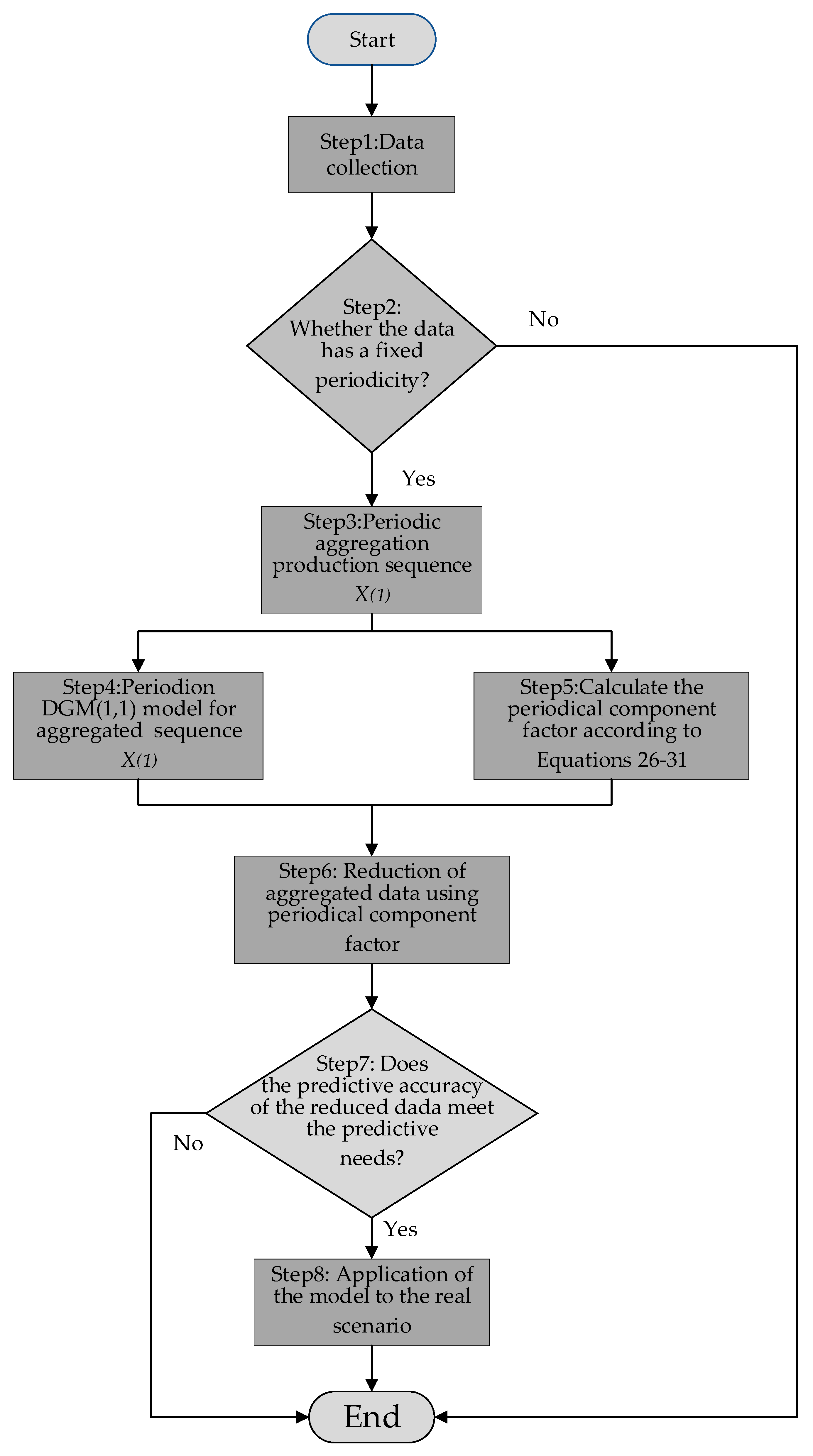
(1) A new seasonal grey prediction model based on periodical aggregation and periodical component factors is proposed. Based on the data-driven perspective, the model improves the existing seasonal grey prediction model by utilizing the grey prediction theory, data preprocessing technology, and seasonal factor theory, and proves the superiority and validity of the newly proposed model through a comparative analysis of two cases.

(2) Based on the classical seasonal grey model, which cannot effectively explore the potential information of seasonal time series, making the model’s interpretability low, the model structure complicated, and technical implementation difficult, the newly proposed model is based on the data preprocessing method of periodical aggregation, which effectively uses the characteristics of periodical seasonal data and constructs a model with a simple structure and strong interpretability of the prediction steps, solving the problems of the existing classical seasonal grey forecasting model to a certain extent.

2. Relevant Concepts and Methods

2.1. Periodical Seasonal Series

Periodical fluctuation series is a common form of time series in sales, financial, and other widely available data.

Definition 1.

Let the sequence $X=\left(x\left(1\right),x\left(2\right),\dots ,x\left(n\right)\right),$for $\forall k\in \{\mathrm{2,3},\dots ,n\},$ If $x\left(k\right)>x\left(k-1\right),$then $X$ is said to be a monotone increasing sequence; If $x\left(k\right)<x(k-1)$, then$X$ is said to be a monotonically decreasing sequence; $X$ is said to be a fluctuating sequence if $\exists k,$such that $\left[x\right(k)-x(k-1\left)\right]\cdot \left[x\right(k+1)-x(k\left)\right]<0.$

Definition 2.

According to Definition 1, if a sequence $X$ is a fluctuating sequence and there exists a period $T$ = 4 or $T$ = 12 for $\forall k\in \left\{\mathrm{2,3},\dots ,n\right\}, X$ always satisfies $x\left(k+nT\right)>x\left(k+\left(n-1\right)T\right);$ or $x(k+nT)<x(k+(n-1\left)T\right)$; or $x(k+nT)\approx x(k+(n-1\left)T\right),$ then the sequence $X$ is said to be a quarterly- or monthly-based cyclic seasonal fluctuation series [49].

2.2. Comparative Models

2.2.1. Holt–Winters Model

The Holt–Winters model is a classic method for predicting seasonal time series and can accurately capture trends and seasonal variations. The model was proposed by Charles Holt and Peter Winters in 1960 and has been improved and extended many times to become a widely used predicting method [50]. The Holt–Winters model is based on three components, which are the trend, seasonality, and seasonal error [51]. The basic form of the model can be categorized into the following three types: simple exponential smoothing, quadratic exponential smoothing, and triple exponential smoothing [52].

The simple exponential smoothing method is suitable for data without significant trends and seasonal variations. This method applies the decreasing weight of past observations to the calculation of the predicted values by exponentially smoothing historical data to obtain prediction results for the future period. The quadratic exponential smoothing method applies to data with a trend but without seasonal changes [53]. Based on the quadratic exponential smoothing method, the triple exponential smoothing method introduces seasonal smoothing, which can better predict seasonal fluctuation data [54]. Given the smoothing coefficient, $\alpha \in \left[\mathrm{0,1}\right]$, then the formula for triple exponential smoothing is as follows:

$$\begin{array}{c}{S}_t^{\left(1\right)}=\alpha x_t+(1-\alpha )S_{t-1}^{\left(1\right)}\\ S_t^{\left(2\right)}=\alpha S_t^{\left(1\right)}+(1-\alpha )S_{t-1}^{\left(2\right)}\\ S_t^{\left(3\right)}=\alpha S_t^{\left(2\right)}+(1-\alpha )S_{t-1}^{\left(3\right)}\end{array}$$

(1)

The formula for predicting the value $x_{t+T}$ for the next $T$ period is as follows:

$$x_{t+T}=A_T+B_{T}T+C_T{T}^2$$

(2)

$$A_t=3S_t^{\left(1\right)}-3S_t^{\left(2\right)}+S_t^{\left(3\right)}$$

(3)

$$B_t=\left({\displaystyle \frac{\alpha }{2(1-\alpha {)}^2}}\right)\left[\right(6-5\alpha )S_t^{\left(1\right)}-2(5-4\alpha )S_t^{\left(2\right)}+(4-3\alpha \left)S_t^{\left(3\right)}\right]$$

(4)

$$C_t=\left({\displaystyle \frac{{\alpha }^2}{2(1-\alpha {)}^2}}\right)[S_t^{\left(1\right)}-2S_t^{\left(2\right)}+S_t^{\left(3\right)}]$$

(5)

2.2.2. EMD-DGM Model

The EMD-DGM framework evolves from conventional seasonal grey modeling by integrating empirical mode decomposition with seasonal adjustment mechanisms while incorporating methodological refinements guided by domain-specific meteorological assumptions to enhance hybrid forecasting architectures [40].

Assumption 1.

Based on China’s national renewable energy strategic planning, renewable energy systems exhibit persistent developmental progression governed by institutionalized policy frameworks.

Assumption 2.

The spatiotemporal distribution characteristics of RES infrastructure, dictated by regional climatic periodicities and geographical siting constraints, manifest predominantly as seasonal variations with time-invariant intra-annual cyclical patterns.

Assumption 3.

The exposure to non-periodical impacts and stochastic irregularities are minor and do not cause system changes.

Building upon the established theoretical framework, the EMD-DGM methodology preserves the intrinsic trend component’s quasi-exponential growth pattern while implementing the additive decomposition of cyclical constituents—seasonal variation S(t), periodic fluctuation C(t), and stochastic residual R(t). This synthesis procedure systematically eliminates aperiodic interferences and stochastic anomalies through harmonic synthesis, ultimately deriving the consolidated periodic disturbance operator I(t), as formalized as follows:

$$I\left(t\right)=S\left(t\right)+C\left(t\right)+R\left(t\right),t\in z$$

(6)

After reorganization, the multiplicative and additive models are as follows:

$$Y^{\mathrm{*}}\left(t\right)=I\left(t\right)+S\left(t\right),t\in z$$

(7)

$$Y^{\mathrm{*}}\left(t\right)=I\left(t\right) \mathrm{\ast } S\left(t\right),t\in z$$

(8)

Given the demonstrated superior adaptability of multiplicative decomposition in empirical implementations, the EMD-DGM framework employs a multiplicative architecture for subsequent modeling phases. Within this paradigm, the periodic disturbance operator I(t) is conceptualized as a seasonal modulation factor acting upon the core trend component. For temporal observations spanning T discrete intervals, we formalize the parameterization through k dominant periodicities and m seasonal constituents, with the seasonal modulation operator derived as follows:

$$I_m\left(t\right)={\displaystyle \frac{\sum _{i=\mathrm{ }1}^{i=\mathrm{ }n}{Y^{\mathrm{*}}\left(kt\right)}^p}{\sum _{i=\mathrm{ }1}^{i=\mathrm{ }n}{S\left(kt\right)}^p}}$$

(9)

where $t$ denotes each time point in period $t=\mathrm{1,2},\mathrm{3,4}\dots n$. There are $k$periods, $k=\mathrm{1,2},\mathrm{3,4}\dots .n$. $p$ denotes the same seasonal component under different periods, $p=\mathrm{1,2},\mathrm{3,4}\dots .m$. $\sum _{i=1}^{i=n}{Y^{\mathrm{*}}\left(kt\right)}^p$ denotes the cumulative value of the same seasonal component for different periods under$t$ time points of the original data. $\sum _{i=1}^{i=n}{S\left(kt\right)}^p$ denotes the cumulative value of the same seasonal components of different periods of the trend component for t time points of the decomposed data [49].

The EMD-DGM model decomposes and reorganizes the data according to Assumptions 1–3 and Equations (6)–(8). Since the trend component after decomposition and reorganization has obvious “quasi-exponentiality” characteristics, the EMD-DGM model utilizes the DGM (1,1) to predict the trend component, calculates the seasonal factor $I\left(t\right)$ by using Equation (9), then uses the seasonal factor $I\left(t\right)$ to correct DGM (1,1), and finally completes the integration and prediction of the model to establish the EMD-DGM model. The algorithm flow is shown in

Table 2. EMD-DGM model algorithm flow [40].

	Steps
Initial	Initialize the software.
Step 1	Collecting data.
Step 2	EMD decomposition of the data.
Step 3	Determine if the raw data are effectively separated, if they are, go to the next step, if they are not, the algorithm ends.
Step 4	Data reorganization according to time series component theory.
Step 5	Indeed, whether the reorganized time series satisfies the characteristics of the trend term and the seasonal fluctuation term, and if not, reorganize it.
Step 6	DGM (1,1) modeling of trend components for trend prediction.
Step 7	Based on the isolation of the seasonal fluctuation component from the raw data and using Equations (6)–(9), the seasonal factor $I\left(t\right)$ is calculated.
Step 8	Seasonal factor is used to adjust the fitted and predicted values of the DGM model.
Step 9	Obtain adjusted fitted and predicted values.
Step 10	Determine whether the fitting accuracy and prediction accuracy of the model meet the requirements, if so, go to the next step, if not, the algorithm ends.
Step 11	Applying the model to specific case studies.
End	Export specific data.

.

2.2.3. SARIMA Model

The SARIMA (Seasonal ARIMA) model is an extended version of the ARIMA model proposed in Box and Jenkins, which is widely used in seasonal time series analysis and forecasting [55]. A time series $\left\{\mathrm{X}t\right|\mathrm{t}=\mathrm{1,2}, \dots , \mathrm{N}\}$, is controlled by SARIMA $(p,d,q)\times (P,D,Q)$ and an additional seasonal period parameter s. The seven parameters can be divided into two categories, three non-seasonal parameters $(p,d,q)$, and four seasonal parameters $(P,D,Q,s)$, where $d$ is the non-seasonal difference order, $s$ is the length of the seasonal period, $p$ is the non-seasonal autoregressive order, and $q$ is the non-seasonal moving average. The SARIMA model with the order $(p,d,q)\times (P,D,Q, s)$ is structured as follows [55]:

$${\varphi }_p\left(B\right){\mathsf{\Phi }}_P\left(B^s\right)(1-B{)}^d{\left(1-B^s\right)}^D{x}_t={\theta }_q\left(B\right){\mathsf{\Theta }}_Q\left(B^s\right){\epsilon }_t$$

(10)

where

$$\begin{array}{c}{\varphi }_p\left(B\right)=1-{\varphi }_{1}B-\dots -{\varphi }_p{B}^p\\ {\theta }_q\left(B\right)=1-{\theta }_{1}B-\dots -{\theta }_q{B}^q\\ {\mathsf{\Phi }}_P\left(B^s\right)=1-{\mathsf{\Phi }}_1{B}^s-\dots -{\mathsf{\Phi }}_p{B}^{Ps}\\ {\mathsf{\Theta }}_Q\left(B^s\right)=1-{\mathsf{\Theta }}_1{B}^s-\dots -{\mathsf{\Theta }}_Q{B}^{Qs}\end{array}$$

(11)

$\left\{x_t\right\}$ is the original time series sequence and $\left\{{\epsilon }_t\right\}$ is an independent, zero-mean, homoskedastic white noise sequence, where $P$ is the seasonal autoregressive order and $Q$ is the seasonal moving average order. ${\theta }_1,{\theta }_2,\dots ,{\theta }_q,{\mathsf{\Theta }}_1,\dots ,{\mathsf{\Theta }}_Q,{\varphi }_1,\dots ,{\varphi }_p,{\mathsf{\Phi }}_1,\dots ,{\mathsf{\Phi }}_P$ are the unknown parameters in the model.

2.2.4. DGGM (1,1) Model

The traditional GM (1,1) model is suitable for the study of time series with small fluctuations. Time series data with obvious seasonal characteristics fluctuate more, and the direct establishment of GM (1,1) using the overall data is less adaptive, so the DGGM (1,1) model is optimized by using data grouping, which makes the model adaptive to the seasonal time series. Compared with the traditional GM (1,1) modeling process, two steps are added to the optimized DGGM (1,1) model [47].

First, the time series data are divided into quarters to generate the sequence $x^{\left(0\right)}\left(s\right)\left(x^{\left(0\right)}\right(s,1),x^{\left(0\right)}(s,2),\dots ,x^{\left(0\right)}(s,n\left)\right),s=\mathrm{1,2},\mathrm{3,4}$. Secondly, the original data $x^{\left(0\right)}\left(s\right)=\left(x^{\left(0\right)}\right(s,1),x^{\left(0\right)}(s,2),\dots ,x^{\left(0\right)}(s,n\left)\right),s=\mathrm{1,2},\mathrm{3,4}$ are accumulated to generate the cumulative sequence $x^{\left(1\right)}\left(s\right)$. Then, GM (1,1) models are built using grouped cumulative data $x^{\left(1\right)}\left(s\right)$ as the original time series, respectively [47].

$$\begin{gathered} x^{\left(1\right)}\left(s\right)=\left(x^{\left(1\right)}\left(s,1\right),x^{\left(1\right)}\left(s,2\right),\dots x^{\left(1\right)}\left(s,n\right)\right) \\ =\left(x^{\left(1\right)}\left(s,1\right),x^{\left(1\right)}\left(s,1\right)+x^{\left(0\right)}\left(s,2\right),\dots x^{\left(1\right)}\left(\mathrm{s},n-1\right)+x^{\left(0\right)}\left(\mathrm{s},n-1\right)\right),s=1, 2, 3, 4 \end{gathered}$$

(12)

where $x^{\left(1\right)}\left(s,k\right)=\sum _{i=1}^k{x}^{\left(0\right)}\left(s,i\right),k=\mathrm{1,2}\dots ,n;s=1, 2, 3, 4$ and the mean rank is $z^{\left(1\right)}\left(s,k\right)=0.5x^{\left(1\right)}\left(s,k\right)+0.5x^{\left(1\right)}\left(s,k-1\right),k=2, 3,\dots ,n;s=1, 2, 3, 4$. Taking the first-order differential equation of a single variable as the predictive model, the grey differential equation is obtained, given by $x^{\left(0\right)}\left(s,k\right)+a{z}^{\left(1\right)}\left(s,k\right)=b,k=\mathrm{2,3},\dots ,n;s=1, 2, 3, 4$. The corresponding whitened differential equation is as follows [47]:

$${\displaystyle \frac{d{x}^{\left(1\right)}(s,t)}{dt}}+a{x}^{\left(1\right)}(s,t)=b$$

(13)

2.3. Model Comparison Indicators

To verify the predictive performance of the model, it is also necessary to establish appropriate criteria to determine the validity of the results. Therefore, to accurately and effectively reveal the differences between the actual observations and the estimated values, this paper divides the data into training and testing sets and also selects the absolute percentage error (APE), mean absolute percentage error (MAPE), mean absolute error (MAE), and root mean square error (RMSE) to measure the accuracy of the model training and prediction results. The relevant formulas for their calculation are as follows:

$$APE=\left|{\displaystyle \frac{e\left(i\right)}{x^{\left(0\right)}\left(i\right)}}\right|\times 100\%$$

(14)

$$MAPE={\displaystyle \frac{1}{n}}{\sum }_{i=\mathrm{ }1}^n\left|{\displaystyle \frac{e\left(i\right)}{x^{\left(0\right)}\left(i\right)}}\right|\times 100\%$$

(15)

$$RMSE=\sqrt{{\displaystyle \frac{1}{n}}{\sum }_{i=1}^n{e}^{\left(2\right)}\left(i\right)}$$

(16)

$$MAE={\displaystyle \frac{1}{n}}{\sum }_{i=\mathrm{ }1}^n|e\left(i\right)|$$

(17)

where $x^{\left(0\right)}\left(i\right)$ is the true value, ${\hat{x}}^{\left(0\right)}\left(i\right)$ is the predicted value, and $e\left(i\right)=x^{\left(0\right)}\left(i\right)-{\hat{x}}^{\left(0\right)}\left(i\right)$.

The root mean square error (RMSE) is a commonly used measure of the difference between the predicted and observed values of a model, which is used to assess how well the model fits the given data. The RMSE is obtained by calculating the mean of the squares of the differences between the predicted values and the actual observations and taking the square root of the squares. The smaller the value is, the better the model fits the data, and the better the model’s performance in predicting the data. The mean absolute error (MAE) is calculated as the average of the absolute difference between the actual value and the predicted value, and is used to measure the average proximity between the predicted value and the actual value; the lower the MAE, the higher the accuracy, and zero means the prediction is perfect. For the MAPE value, in the training set, if the value is smaller, it means that the model fits better and is more adaptable; in the test set, if the value is smaller, it means that the model has a higher prediction accuracy and the prediction results are more convincing. The grading criteria shown in

Table 3. Prediction accuracy grading scale.

MAPE (%)	Predicted Effects	MAPE (%)	Predicted Effects
<10	Good	20–50	Wrong
10–20	General	>50	Very wrong

are usually followed [56].

3. Seasonal Grey Prediction Model Based on Periodic Aggregation and Periodic Component Factor

3.1. DGM (1,1) Model

The conventional GM (1,1) approach exhibits a persistent conceptual challenge in grey system theory—the non-trivial transition between its discrete formulation and continuous whitening equation representation. Addressing this fundamental discontinuity, the DGM (1,1) establishes axiomatic foundations through strict discrete-to-discrete formalism, resolving the theoretical incongruence while developing a self-consistent discrete prediction architecture [49].

In the traditional GM (1,1) model, the jump from the discrete form of the model to the continuous form of the whitening equation has always troubled researchers in grey system theory. The DGM (1,1) model takes this as the starting point of research to solve this theoretical problem from discrete to discrete and establishes a discrete grey prediction model [49,57].

Definition 3.

Let ${ x}^{\left(0\right)}$ denote a non-negative primitive time series, with its first-order accumulated generating operation (1-AGO) series $x^{\left(1\right)}$ constructed through cumulative summation.

$$\begin{array}{c}{X}^{\left(0\right)}=\left(x^{\left(0\right)}\left(1\right),x^{\left(0\right)}\left(2\right),\dots ,x^{\left(0\right)}\left(n\right)\right)\\ X^{\left(1\right)}=\left(x^{\left(1\right)}\left(1\right),x^{\left(1\right)}\left(2\right),\dots ,x^{\left(1\right)}\left(n\right)\right)\end{array}$$

(18)

which $x^{\left(0\right)}\left(k\right)\ge 0,x^{\left(1\right)}\left(k\right)=\sum _{i=1}^k{x}^{\left(0\right)}\left(i\right), k=1, 2,\dots ,n$, called

$$x^{\left(1\right)}(k+1)={\beta }_1{x}^{\left(1\right)}\left(k\right)+{\beta }_2$$

(19)

Definition 4.

Let $x^{\left(0\right)}$ and $x^{\left(1\right)}$ denote the sequences established in Definition 3. The parameter column vector is formally expressed as: $\hat{\beta }={[{\beta }_1,{\beta }_2]}^T$, where the $\beta$ encapsulates the model coefficients to be estimated.

$$Y=\left[\begin{array}{c}{x}^{\left(1\right)}\left(2\right)\\ x^{\left(1\right)}\left(3\right)\\ ⋮\\ x^{\left(1\right)}\left(n\right)\end{array}\right], B=\left[\begin{array}{cc}{x}^{\left(1\right)}\left(1\right)& 1\\ x^{\left(1\right)}\left(2\right)& 1\\ ⋮& ⋮\\ x^{\left(1\right)}\left(n-1\right)& 1\end{array}\right]$$

(20)

Then, the least-squares estimated parameter column $x^{\left(1\right)}(k+1)={\beta }_1{x}^{\left(1\right)}\left(k\right)+{\beta }_2$ satisfying

$$\hat{\beta }={[{\beta }_1,{\beta }_2]}^{\mathrm{T}}={\left(B^{\mathrm{T}}B\right)}^{-1}{B}^{\mathrm{T}}Y$$

(21)

Definition 5.

Assume $Y$ and $B$ are as shown in Definition 4, $\hat{\beta }={\left(B^{T}B\right)}^{-1}{B}^{T}Y$. Let $x^{\left(1\right)}\left(1\right)=x^{\left(0\right)}\left(1\right)$, then $x^{\left(1\right)}(k+1)={\beta }_1{x}^{\left(1\right)}\left(k\right)+{\beta }_2$, the time response equation of the following:

$${\hat{x}}^{\left(1\right)}(k+1)={{\beta }_1}^k\left(x^{\left(0\right)}\right(1)-{\displaystyle \frac{{\beta }_2}{1-{\beta }_1}})+{\displaystyle \frac{{\beta }_2}{1-{\beta }_1}}$$

(22)

where $k=1, 2,\dots ,n-1$. The reduction equation is given by the following equation:

$$x^{\left(0\right)}(k+1)=({\beta }_1-1)\left(x^{\left(0\right)}\right(1)-{\displaystyle \frac{{\beta }_2}{1-{\beta }_1}}){\beta }_1^k,k=\mathrm{1,2},\dots ,n-1.$$

(23)

3.2. PADGM Model Construction

Conventional grey forecasting frameworks demonstrate efficacy in modeling complex systems exhibiting “quasi-exponential” patterns within observational datasets. However, when applied to renewable energy generation forecasting—a multidimensional system characterized by inherent periodic seasonality, nonlinear trends, and stochastic fluctuations—these classical methodologies exhibit a constrained predictive performance. This methodological limitation has driven the development of advanced seasonal grey variants specifically engineered for limited-data scenarios, including but not limited to the DGGM (1,1) framework [57], FOTP-SDGM architecture [58], and SADGM paradigm [47]. With these solution ideas, there are still some considerable limitations. For example, after the model structure is complicated, the number of parameters to be estimated increases, which often requires intelligent algorithms for auxiliary calculations, with considerable technical difficulties. Traditional data preprocessing will destroy the information of the original data and reduce the interpretability of the model, which increases the difficulty of promoting the model in practical application scenarios. To overcome these constraints, the present methodology enhances conventional DGM (1,1) forecasting through optimized preprocessing protocols involving refined data decomposition and seasonal influence mitigation, maintaining structural parsimony and model interpretability as fundamental design principles [39,40,41].

The basic idea of the seasonal grey prediction model constructed by the data decomposition algorithm and seasonal factor is to decompose the trend, periodicity, and stochastic volatility in the original data by using the data decomposition algorithm. Since the trend conforms to the “quasi-exponentiality” law and the traditional grey prediction model can be effectively predicted, the classical grey prediction model can be utilized for the information mining and prediction of the classical grey prediction model. Using the theory of the composition of time series and related seasonal assumptions, periodicity and random volatility are reflected through seasonal factors. By combining seasonal factors with mining trendiness and a grey prediction model, seasonal time series can be effectively mined with a small amount of data, and predicted values with a high interpretation and prediction accuracy can be obtained.

The data decomposition method depends on the selection of data decomposition algorithms, and excellent data decomposition algorithms can better extract the trend terms of periodical seasonal data to obtain accurate seasonal factors for data reduction. Nevertheless, a suboptimal performance of a data decomposition algorithm in handling specific datasets may induce significant prediction deviations. Consequently, this study employs an inverse decomposition methodology for periodic aggregation to capture the intrinsic quasi-exponentiality patterns, with model formulation guided by the following theoretical premises [49].

Assumption 4.

Under China’s institutionalized renewable energy policy frameworks, temporal aggregation operators effectively neutralize seasonal fluctuations, revealing persistent quasi-exponential growth trajectories in longitudinal system dynamics.

Assumption 5.

The spatiotemporal configuration parameters of system components exhibit bounded variability constrained by China’s geographic–climatic determinants, maintaining structural invariance across operational cycles.

Post-aggregation analysis of China’s renewable energy generation datasets confirms statistically significant quasi-exponential pattern emergence (p < 0.01), enabling methodological progression to subsequent analytical phases.

The conventional grey forecasting framework demonstrates an inherent capacity for handling quasi-exponentiality patterns, achieving both fitted and predicted trajectories with controlled error margins through its characteristic differential equation mechanisms. Moreover, the periodical component factor is a process of assigning weights to each periodical component due to the assigned data source of the fitted and predicted values of the traditional grey prediction model. Based on the excellent performance of the grey prediction model, the data reduction based on the weights qualifies the error to a certain extent, increasing the prediction accuracy of the model and the reduction error. The mathematical specification of the PADGM framework proceeds as follows:

Definition 6.

Given a non-negative primitive time series $X^{\left(0\right)}=(X^{\left(0\right)}\left(1\right),X^{\left(0\right)}(2)\dots \dots X^{\left(0\right)}(m\left)\right)$ with predefined periodicity configuration, let n denote the identified periodic components distributed across m complete cycles.

$$X_{mn}=\left[\begin{array}{ccc}{x}_{11}& x_{21}& \begin{array}{cc}\dots & x_{m1}\end{array}\\ x_{12}& x_{22}& \begin{array}{cc}\dots & x_{m2}\end{array}\\ \begin{array}{c}⋮\\ x_{1n}\end{array}& \begin{array}{c}⋮\\ x_{2n}\end{array}& \begin{array}{c}\begin{array}{cc}⋮& ⋮\end{array}\\ \begin{array}{cc}\dots & x_{mn}\end{array}\end{array}\end{array}\right]$$

(24)

Definition 7.

As shown in Definition 6, by each period$m$ perform periodical aggregation, let the data sequence of periodical aggregation be as follows:

$$X^{\left(1\right)}={(X}_1^{\left(1\right)},X_2^{\left(1\right)}{,\dots .X}_m^{\left(1\right)})$$

(25)

where $X_m^{\left(1\right)}=\sum _{n=1}^{n=n}{X}_{mn}.$

Building upon Assumption 5, which posits the temporal stability of period-specific weighting coefficients, these parametric values are computationally derived through the following mathematical formulation:

$$f_{ij}={\displaystyle \frac{X_{ij}}{X_i^{\left(1\right)}}}$$

(26)

where $i$ denotes the data after aggregation of the $m$th cycle of the sequence $X^{\left(1\right)}$, $i=1, 2, 3\dots m$. $j$ denotes the $j$th component under period $i$, $j=1, 2, 3\dots n$. The component weights for each period are calculated and expressed as a matrix in the form of $f_{ij}$, as follows [49]:

$$f_{ij}=\left[\begin{array}{ccc}{f}_{11}& f_{21}& \begin{array}{cc}\dots & f_{i1}\end{array}\\ f_{12}& f_{22}& \begin{array}{cc}\dots & f_{i2}\end{array}\\ \begin{array}{c}⋮\\ f_{1j}\end{array}& \begin{array}{c}⋮\\ f_{2j}\end{array}& \begin{array}{c}\begin{array}{cc}⋮& ⋮\end{array}\\ \begin{array}{cc}\dots & f_{ij}\end{array}\end{array}\end{array}\right]$$

(27)

Definition 8.

Let m denote the total cycle duration and n denote the quantity of periodic components. The temporal sequence $f_{ij}$ is constructed through row-wise aggregation via the summation operator $\sum _{i=1}^{i=m}{f}_{ij}$, yielding the following parametric configuration:

$$f_j=\left[\begin{array}{c}{f}_1\\ f_2\\ ⋮\\ f_j\end{array}\right]\hspace{1em}\hspace{1em}\hspace{1em}j=1, 2, 3\dots n$$

(28)

Subsequently, the $Q_s$ coefficient characterizing the periodic-averaged constituent is as follows:

$$Q_s={\displaystyle \frac{f_j}{{\sum }_{j=1}^{j=n}{f}_j}}$$

(29)

Let $Q_s$ denote the temporal-phase weighted coefficient under complete temporal modulation, where s = 1, 2, 3,…, n indexes discrete phase intervals.

Definition 9.

Let m denote the total temporal span, p represent the quantity of phases influenced by the novel information principle, and n indicate the count of periodic constituents. The differential sequence ${\Delta f}_j$ is generated through cumulative row summation: $\sum _{i=m-p+1}^{i=m}{f}_{ij}$, which has the following form:

$${\mathsf{\Delta }f}_j=\left[\begin{array}{c}{\mathsf{\Delta }f}_1\\ {\mathsf{\Delta }f}_2\\ ⋮\\ \mathsf{\Delta }{f}_j\end{array}\right] j=1, 2, 3,\dots ,n\mathrm{ }$$

(30)

Then, the factor of the new information periodical component $w_s$ under the influence of the $p$-period is as follows:

$$w_s={\displaystyle \frac{{\mathsf{\Delta }f}_j}{{\sum }_{j=1}^{j=n}{\mathsf{\Delta }f}_j}}$$

(31)

Let $w_s$ denote the periodic information modulation coefficient influenced by p-phase cyclical variations, where $s=1, 2, 3,\dots ,n$.

Definition 10.

Given the periodic aggregated sequence $X^{\left(1\right)}={(X}_1^{\left(1\right)},X_2^{\left(1\right)}{,\dots .X}_m^{\left(1\right)}),$ as formalized in Definition 7, the DGM (1,1) modeling framework is implemented through systematic application of Assumption 4 and Equations (18)–(23). This yields the following two distinct temporal outputs:

$$X^{\left(2\right)}=(X^{\left(2\right)}\left(1\right){,X}^{\left(2\right)}\left(2\right),\dots \dots X^{\left(2\right)}(m+k\left)\right)$$

(32)

According to Definitions 8 and 9, let $Q_s$ denote the periodic-averaged component factor and $Q_s$ represent the periodicity-influenced novel information component factor. Where s indicates the quantity of periodic constituents distributed across n temporal intervals, the dimensionally reduced series derived via the periodic-averaged operator $Q_s$ is mathematically expressed as follows:

$$X^{\left(2\right)}=(X^{\left(2\right)}\left(1\right)·Q_{1T}{, X}^{\left(2\right)}(2)·Q_{2T},\dots \dots X^{\left(2\right)}(m+k)·Q_{iT})$$

(33)

where $T=1,2,3\dots .n$,$i=1,2,3,.....s$.

The reduced series using the new information period component factor $w_s$ under the influence of the $p$-period is as follows [49]:

$$X^{\left(2\right)}=(X^{\left(2\right)}\left(1\right)·Q_{11}{, X}^{\left(2\right)}(2)·Q_{21},\dots \dots X^{\left(2\right)}(m+k)·Q_{iT})$$

(34)

where $i=1,2,3.....s$, $T=1,2,3\dots .n$.

Let the reduction matrices be $F$ and $Z$. The period-average component reduction matrix is given by the following:

$$\mathrm{F}=\left[\begin{array}{ccc}{X}^{\left(2\right)}\left(1\right)·Q_1& X^{\left(2\right)}\left(2\right)·Q_1& \begin{array}{cc}\dots & X^{\left(2\right)}(m+k)·Q_1\end{array}\\ X^{\left(2\right)}\left(1\right)·Q_2& X^{\left(2\right)}\left(2\right)·Q_2& \begin{array}{cc}\dots & X^{\left(2\right)}(m+k)·Q_2\end{array}\\ \begin{array}{c}{X}^{\left(2\right)}\left(1\right)·Q_3\\ ⋮\\ X^{\left(2\right)}\left(1\right)·Q_s\end{array}& \begin{array}{c}{X}^{\left(2\right)}\left(2\right)·Q_3\\ ⋮\\ X^{\left(2\right)}\left(2\right)·Q_s\end{array}& \begin{array}{c}\begin{array}{cc}\dots & X^{\left(2\right)}(m+k)·Q_3\\ ⋮& ⋮\end{array}\\ \begin{array}{cc}\dots & X^{\left(2\right)}(m+k)·Q_s\end{array}\end{array}\end{array}\right]$$

(35)

The weight reduction matrix governing the novel information periodic component, subject to p-periodic modulation dynamics, is mathematically formulated as follows:

$$\mathrm{Z}=\left[\begin{array}{ccc}{X}^{\left(2\right)}\left(1\right)·w_1& X^{\left(2\right)}\left(2\right)·w_1& \begin{array}{cc}\dots & X^{\left(2\right)}(m+k)·w_1\end{array}\\ X^{\left(2\right)}\left(1\right)·w_2& X^{\left(2\right)}\left(2\right)·w_2& \begin{array}{cc}\dots & X^{\left(2\right)}(m+k)·w_2\end{array}\\ \begin{array}{c}{X}^{\left(2\right)}\left(1\right)·w_3\\ ⋮\\ X^{\left(2\right)}\left(1\right)·w_s\end{array}& \begin{array}{c}{X}^{\left(2\right)}\left(2\right)·w_3\\ ⋮\\ X^{\left(2\right)}\left(2\right)·w_s\end{array}& \begin{array}{c}\begin{array}{cc}\dots & X^{\left(2\right)}(m+k)·w_3\\ ⋮& ⋮\end{array}\\ \begin{array}{cc}\dots & X^{\left(2\right)}(m+k)·w_s\end{array}\end{array}\end{array}\right]$$

(36)

The calculation process of the model is shown in Figure 2. The proposed methodology demonstrates an enhanced theoretical adaptability and operational simplicity compared to conventional seasonal factors derived from data decomposition frameworks. Methodologically, this approach eliminates dependency on predefined decomposition algorithms while introducing dynamic periodicity weighting mechanisms—contrasting with static seasonal coefficients, the model enables differential weight allocation across temporal intervals, thereby better aligning with information theory’s new information prioritization principle. Furthermore, the streamlined implementation process requires only foundational grey prediction modeling knowledge, effectively circumventing the structural complexities inherent in traditional decomposition-based techniques [49].

4. Case Study

4.1. Case 1

4.1.1. Data Sources and Processing

To accurately evaluate the modeling advantages and flexibility of the PADGM model, Chinese PV power generation data from the spring of 2016 to the winter of 2022 are selected for prediction in this study, and all the data required for modeling are from the National Bureau of Statistics of China. Aligned with China’s latitudinal characteristics, the meteorological seasons are systematically categorized as follows: spring (March–May), summer (June–August), autumn (September–November), and winter (December–February of subsequent years). These seasonal divisions correspond to standardized quarterly designations Q1–Q4, respectively, with complete chronological records spanning from 2016Q1 through to 2022Q4, as documented in

Table 4. PV power generation in China (2016Q1–2022Q4).

Year/Quarter	Q1	Q2	Q3	Q4
2016	94	111.6	106.7	109.5
2017	152.9	181.4	181.5	188.3
2018	215.2	228.1	255.5	211.8
2019	313.9	323.6	307.1	259.3
2020	394	374.1	360.3	360.1
2021	447.9	509.7	491.9	435.1
2022	592.5	648.5	549.3	531.2

and visualized in Figure 3.

From Figure 3, it is obvious that China’s PV power generation has an obvious trend and periodicity volatility, with great seasonal differences, roughly presenting the seasonal general law of Q2 > Q3 > Q2 > Q4, showing, overall, a spiral upward trend in recent years. Among them, this study employs wind power generation data spanning 2016Q1–2021Q4 (24 quarterly observations) for model calibration, with subsequent measurements from 2022Q1–2022Q4 allocated for predictive validation.

4.1.2. PADGM Model Construction

To verify the prediction accuracy and advantages of the proposed model, 2016Q1–2021Q4 PV power generation is selected as the training set and 2022Q1–2022Q4 as the test set. The Holt–Winters model and EMD-DGM model are established as the comparison models. Three indicators, MAE, RMSE, and MAPE, are chosen as the evaluation criteria for comparing the accuracy of the models. The prediction model proposed in this paper is first fitted. To verify the flexibility of the PADGM model in this chapter, two types of component factors will be used to calculate the model.

In this paper, the training set of PV power generation data is firstly organized into a matrix form with a periodical component of four and a period of six by Definition 6 and Equation (24). Its matrix form is as follows:

$$X_{\mathrm{6,4}}=\left[\begin{array}{cc}\begin{array}{ccc}94& 152.9& \begin{array}{cc}215.2& 313.9\end{array}\\ 111.9& 181.4& \begin{array}{cc}228.1& 323.6\end{array}\\ \begin{array}{c}106.7\\ 109.5\end{array}& \begin{array}{c}181.5\\ 188.3\end{array}& \begin{array}{c}\begin{array}{cc}255.5& 307.1\end{array}\\ \begin{array}{cc}211.8& 259.3\end{array}\end{array}\end{array}& \begin{array}{cc}394& 447.9\mathrm{ }\\ 374.1& 509.7\mathrm{ }\\ \begin{array}{c}360.3\mathrm{ }\\ 360.1\mathrm{ }\end{array}& \begin{array}{c}491.9\mathrm{ }\\ 435.1\mathrm{ }\end{array}\end{array}\end{array}\right]$$

According to Definition 7 and Equation (25), it is periodically aggregated to obtain the periodical aggregation serial, as follows:

$$X^{\left(1\right)}=\left[\begin{array}{ccc}421.8& 704.1& \begin{array}{ccc}910.6& 1203.9& \begin{array}{cc}1488.5& 1884.6\end{array}\end{array}\end{array}\right]$$

As in Figure 4, the “quasi-exponentiality” characterization of the raw data is strengthened by data preprocessing such as periodical aggregation.

Due to the obvious “quasi-exponentiality” characteristics of the aggregated data, the traditional grey prediction model has a good predictive ability. For the preliminary fitting of the DGM (1,1) model to the periodically aggregated data according to Definition 10 and Equations (18)–(23), the fitting formula is as follows:

$$x^{\left(1\right)}(k+1)=1.26x^{\left(1\right)}\left(k\right)+629.69, k=1,\mathrm{ }2,\dots ,n-1.$$

(37)

Equation (37) was used to predict for the year 2022. The results of the fitting and prediction are shown in

Table 5. Fitted and predicted values.

Type	Year	Value
Fitted value	2016	421.8
	2017	723.947
	2018	921.095
	2019	1171.932
	2020	1491.077
	2021	1897.133
Predicted value	2022	2413.768

.

According to Assumption 5, the component weights of each period remain unchanged or do not change much, and the component weights of each period can be obtained through the calculation, which, in turn, leads to the distribution of the component coefficients of each period. According to Definition 7 and Equations (26) and (27), the component weights of each historical period are obtained. The weight of each historical period component of PV power generation during 2016Q1–2021Q4 is as follows:

$$f_{\mathrm{6,4}}=\left[\begin{array}{cccccc}0.2228& 0.2171& 0.2363& 0.2607& 0.2646& 0.2376\\ 0.2645& 0.2576& 0.2504& 0.2687& 0.2513& 0.2704\\ 0.2529& 0.2577& 0.2805& 0.2550& 0.2420& 0.2610\\ 0.2596& 0.2674& 0.2325& 0.2153& 0.2419& 0.2308\end{array}\right]$$

As shown in Figure 5, the periodical component weight matrix allows us to observe how the periodical component weights change in each period.

In turn, the period-averaged component factor serial is obtained according to Definition 8 and Equations (28) and (29), as follows:

$$Q_s=\left[\begin{array}{c}0.2401\\ 0.2606\\ \begin{array}{c}0.2583\\ 0.2410\end{array}\end{array}\right]$$

Then, the periodical weights for 2018–2021 are again used to obtain the mean values, and we follow Definition 9 and Equations (30) and (31) to obtain the serial of the periodical component factor under the influence of the $p$-period, as follows:

$$W_s=\left[\begin{array}{c}0.2411\\ 0.2608\\ \begin{array}{c}0.2515\\ 0.2463\end{array}\end{array}\right]$$

After comparison, this paper finds that the period-averaged component factor serial has no significant mutation compared to the new information periodical component factor serial under the influence of the $p$-cycle. To compare the effectiveness of the two kinds of periodical component factor weights, this paper will use the period-average factor $Q_s$ and the new information periodical component factor $w_s$ as the values of the DGM (1,1) model fitting for the prediction of data reduction, according to Definition 10 and Equations (32)–(36), to obtain the two kinds of periodical component factor under the data reduction. The data reduction is as follows in

Table 6. PV power generation data reduction.

Type	Year	Average Factor Reduction (GWh)	New Information Factor Reduction (GWh)
Fitted value	2016Q1	101.28	107.33
	2016Q2	109.92	111.17
	2016Q3	108.91	106.60
	2016Q4	101.69	96.70
	2017Q1	173.83	184.21
	2017Q2	188.67	190.81
	2017Q3	186.92	182.96
	2017Q4	174.54	165.97
	2018Q1	221.16	234.38
	2018Q2	240.05	242.77
	2018Q3	237.82	232.79
	2018Q4	222.07	211.17
	2019Q1	281.39	298.20
	2019Q2	305.42	308.88
	2019Q3	302.58	296.18
	2019Q4	282.54	268.67
	2020Q1	358.02	379.41
	2020Q2	388.59	393.00
	2020Q3	384.99	376.84
	2020Q4	359.49	341.84
	2021Q1	455.51	482.73
	2021Q2	494.41	500.02
	2021Q3	489.83	479.46
	2021Q4	457.38	434.93
Predicted value	2022Q1	579.56	614.19
	2022Q2	629.05	636.18
	2022Q3	623.22	610.03
	2022Q4	581.94	553.37

.

4.1.3. Comparative Model Construction

Based on Equations (1)–(5), a Holt–Winters model in multiplicative form was constructed using Eviews10. The fit indices of the Holt–Winters model are shown in

Table 7. Holt–Winters model parameters.

	Estimation	Standard Error	T	Significance
Alpha (Level)	0.18	0.10	1.87	0.08
Gamma (Trends)	0.71	0.52	1.37	0.19
Delta (Season)	0.14	0.09	1.61	0.12

.

According to Equations (6)–(8), data decomposition is performed using the EMD algorithm in Matlab software (R2020a), and data reorganization is carried out using the relevant theories. The decomposed and reorganized data are shown in

Table 8. Data after EMD decomposition and reorganization.

Year	Trend Components	Periodic Component	Year	Trend Components	Periodic Component
2016Q1	93.37	0.63	2019Q1	282.26	31.64
2016Q2	99.82	11.78	2019Q2	295.05	28.55
2016Q3	112.71	−6.01	2019Q3	310.28	−3.18
2016Q4	128.19	−18.69	2019Q4	322.77	−63.47
2017Q1	145.63	7.27	2020Q1	341.62	52.38
2017Q2	167.02	14.38	2020Q2	358.34	15.76
2017Q3	185.11	−3.61	2020Q3	378.40	−18.10
2017Q4	200.29	−11.99	2020Q4	403.98	−43.88
2018Q1	211.61	3.59	2021Q1	433.09	14.81
2018Q2	224.18	3.92	2021Q2	463.71	45.99
2018Q3	242.39	13.11	2021Q3	491.10	0.80
2018Q4	261.15	−49.35	2021Q4	504.80	−69.70

.

Using the Equation (9), the seasonal factors are calculated according to

Table 9. Seasonal factors.

Q1	Q2	Q3	Q4
1.0690	1.0720	0.9834	0.8656

.

A DGM (1,1) model is fitted to the decomposed trend components, and the fitted equation is as follows:

$$x^{\left(1\right)}(k+1)=1.1x^{\left(1\right)}\left(k\right)+101.23, k=\mathrm{1,2},\dots ,n-1.$$

(38)

The data were reduced using Equation (38), and then the DGM (1.1) model data were corrected using the seasonal factor from

Table 10. Model comparison based on PV generation data for 2016Q1–2022Q4.

Time	Actual Value	EMD-DGM		Holt-Winters		Periodic Average PADGM		New Information PADGM
		Forecasted Value	Error (%)	Forecasted Value	Error (%)	Forecasted Value	Error (%)	Forecasted Value	Error (%)
Training Set
2016Q1	94	99.82	0.06	97.1	0.03	101.28	0.08	107.33	0.14
2016Q2	111.6	133.08	0.19	112.26	0.01	109.92	0.02	111.17	0
2016Q3	106.7	141.16	0.32	117.68	0.1	108.91	0.02	106.6	0
2016Q4	109.5	120.96	0.1	113.44	0.04	101.69	0.07	96.7	0.12
2017Q1	152.9	162.19	0.06	165.45	0.08	173.83	0.14	184.21	0.2
2017Q2	181.4	183.82	0.01	173.37	0.04	188.67	0.04	190.81	0.05
2017Q3	181.5	168.03	0.07	169.78	0.06	186.92	0.03	182.96	0.01
2017Q4	188.3	178.25	0.05	163.58	0.13	174.54	0.07	165.97	0.12
2018Q1	215.2	221.21	0.03	242.7	0.13	221.16	0.03	234.38	0.09
2018Q2	228.1	236.16	0.04	252.69	0.11	240.05	0.05	242.77	0.06
2018Q3	255.5	232.98	0.09	235.01	0.08	237.82	0.07	232.79	0.09
2018Q4	211.8	216.15	0.02	224.38	0.06	222.07	0.05	211.17	0
2019Q1	313.9	284.2	0.09	298.42	0.05	281.39	0.1	298.2	0.05
2019Q2	323.6	303.4	0.06	315.55	0.02	305.42	0.06	308.88	0.05
2019Q3	307.1	299.33	0.03	306.5	0	302.58	0.01	296.18	0.04
2019Q4	259.3	277.7	0.07	280.34	0.08	282.54	0.09	268.67	0.04
2020Q1	394	365.12	0.07	371.9	0.06	358.02	0.09	379.41	0.04
2020Q2	374.1	389.79	0.04	388.8	0.04	388.59	0.04	393	0.05
2020Q3	360.3	384.55	0.07	366.3	0.02	384.99	0.07	376.84	0.05
2020Q4	360.1	356.77	0.01	325.33	0.1	359.49	0	341.84	0.05
2021Q1	447.9	469.08	0.05	456.08	0.02	455.51	0.02	482.73	0.08
2021Q2	509.7	500.78	0.02	463.07	0.09	494.41	0.03	500.02	0.02
2021Q3	491.9	494.05	0	454.34	0.08	489.83	0	479.46	0.03
2021Q4	435.1	458.36	0.05	426.41	0.02	457.38	0.05	434.93	0
Test set
2022Q1	592.5	602.64	0.02	562.19	0.05	579.56	0.02	614.19	0.04
2022Q2	648.5	643.37	0.01	612.48	0.06	629.05	0.03	636.18	0.02
2022Q3	549.3	628.33	0.14	604.21	0.1	633.22	0.13	610.03	0.11
2022Q4	531.2	578.87	0.09	554.4	0.04	581.94	0.1	553.37	0.04

to finalize the decomposition, integration, and prediction of the data.

4.1.4. Comparison of Model Indicators

For comparison, 2016Q1–2021Q4 were selected as the training set and 2022Q1–2022Q4 were selected as the test set. The Holt–Winters model and EMD-DGM model were used as the comparison models for PV power generation data. According to Equations (14)–(17), the three metrics MAE, RMSE, and MAPE were calculated as the evaluation criteria for comparing the model accuracy, respectively. After calculation, the actual values, predicted values, and errors obtained from the comparison of models on the PV power generation data set are shown in Table 10, the evaluation results of the metrics are shown in Figure 6, and the distribution of the predicted and actual values of the comparison models is shown in Figure 7.

The Holt–Winters model, as a classic model for predicting seasonal time series, can precisely portray time series with trends and seasonal changes. In this model comparison, its MAPE value is 0.06 in both the training and test sets, which is a satisfactory performance. However, observing the MAE value and RMSE value, it can be found that the model fits better in the training set but not in the test set, which shows that the Holt–Winters model does not have an advantage in portraying the trend in the test set. In addition, observation of the fitting graph reveals that there is a large deviation in its fitting performance at the beginning stage, indicating that the stability of the model is doubtful.

The EMD-DGM model uses EMD data decomposition and time series component theory, and by disassembling and reorganizing the series into trend terms and random fluctuation terms, the model minimizes the accumulation of errors due to reduction errors, while the intrinsic evolutionary law of the series is deeply excavated to the achieve accurate prediction of the model. In this study, the MAPE value of the EMD-DGM model is 0.06 in both the training set and the test set, which is a relatively satisfactory performance, basically equal to the Holt–Winters model. The comparative indexes RMSE and MAE are lower than those of the Holt–Winters model in both the training set and the training set, which shows that the stability of the EMD-DGM model is greater than that of the Holt–Winters model. Overall, the overall performance of the EMD-DGM model is completely better than that of the Holt–Winters model.

For the PADGM model based on the new information period component factor in the model comparison based on PV power generation data, in the training set, the MAPE values are 0.05 and 0.06, which are excellent. In the test set, the MAE and RMSE values of the PADGM model based on the new information period component factor are 29.23 and 34.65, which are ranked the first among the models and are much smaller than the values of other models. From the fitted plots of the compared models, the model is more accurate in characterizing the seasonal trends and key turning points of the serial data. In conclusion, the model comparison analysis proves the effectiveness of the methodology proposed in the previous section.

4.2. Case 2

4.2.1. Data Sources and Processing

In this section of the study, China’s wind power generation records spanning from March 2010 to February 2023, obtained from the National Bureau of Statistics (NBS), are used as empirical validation data. Meteorological seasonality is defined according to latitudinal climatic norms, as follows: Q1 (March–May), Q2 (June–August), Q3 (September–November), and Q4 (December–February), with quarterly intervals systematically labeled as 2010Q1–2022Q4 (

Table 11. Quarterly data on wind power generation in China [49].

Year/Quarter	Q1	Q2	Q3	Q4
2010	103.2	103.5	112.2	158.1
2011	206.3	173.4	167.1	195.8
2012	230.5	211.2	237.8	269.5
2013	331.4	283.3	318.3	315.3
2014	365.3	300	345.2	402.2
2015	468	350.9	408	444
2016	585.5	458.8	533.2	597.5
2017	718.3	559.5	711.2	839
2018	918.9	649.2	745.4	909.9
2019	1037.8	701.3	845.1	952.4
2020	1192.4	887.2	996	1323.7
2021	1449.5	1087.7	1321.4	1513.3
2022	1895	1443.3	1691.4	2059.8

). The dataset is partitioned into a calibration subset (2010Q1–2021Q4, 48 quarters) for model development and a validation subset (2022Q1–2022Q4, 3 quarters) for predictive performance evaluation.

4.2.2. Model Construction

In this paper, the DGGM (1,1) model based on seasonal grouping and the SARIMA model are used as comparative models. In this case, the seasonally grouped DGGM (1,1) model is constructed as a GM (1,1) model, and the time response equation of the DGGM (1,1) model is based on Equations (12) and (13) [49], as follows:

$${\displaystyle \frac{d{x}^{\left(1\right)}(1,t)}{dt}}-0.19x^{\left(1\right)}(1,t)=190.95$$

(39)

$${\displaystyle \frac{d{x}^{\left(1\right)}(2,t)}{dt}}-0.18x^{\left(1\right)}(2,t)=149.48$$

(40)

$${\displaystyle \frac{d{x}^{\left(1\right)}(3,t)}{dt}}-0.18x^{\left(1\right)}(3,t)=171.11$$

(41)

$${\displaystyle \frac{d{x}^{\left(1\right)}(4,t)}{dt}}-0.19(4,t)=181.78$$

(42)

Using Equations (39)–(42), the simulation and prediction of the data are achieved. Based on Eviews10 and Equations (10) and (11), the SARIMA (0,1,0) (1,1,0) model is constructed, and the specific fitting indicators are shown in

Table 12. Fitting indicators.

Steady R-Square	R-Square	DF	Significance
0.15	0.98	17.00	0.64

and

Table 13. SARIMA model parameters.

	Estimation	Standard Error	T	Significance
Discrepancy	1.00
AR · seasonality	(0.53)	0.14	(3.86)	0.00
Seasonal differences	1.00

.

The PADGM model constitutes a seasonal grey forecasting framework operationalizing cyclical data aggregation principles. Through rigorous application of Definition 7 and Equation (25), this methodological approach systematically implements cyclical aggregation processing on China’s wind power generation datasets, culminating in the structured formulation of periodical aggregation sequences, as demonstrated as follows:

$$\begin{gathered} {\mathrm{X}}^{\left(1\right)}=(477.0\mathrm{ }\mathrm{ }\mathrm{ }\mathrm{ }742.6\mathrm{ }\mathrm{ }\mathrm{ }\mathrm{ }949.0\mathrm{ }\mathrm{ }\mathrm{ }\mathrm{ }1248\mathrm{ }\mathrm{ }\mathrm{ }\mathrm{ }1412.7\mathrm{ }\mathrm{ }\mathrm{ }\mathrm{ }1670.9\mathrm{ }\mathrm{ }\mathrm{ }\mathrm{ }2175.0 \\ 2828.0\mathrm{ }\mathrm{ }\mathrm{ }\mathrm{ }2828.0\mathrm{ }\mathrm{ }\mathrm{ }\mathrm{ }3223.4\mathrm{ }\mathrm{ }\mathrm{ }\mathrm{ }3536.6\mathrm{ }\mathrm{ }\mathrm{ }\mathrm{ }4399.3\mathrm{ }\mathrm{ }\mathrm{ }\mathrm{ }5371.9) \end{gathered}$$

The serial $X^{\left(1\right)}$ is simulated and predicted using the DGM (1,1) model fitted by Equations (18)–(23), as follows:

$$x^{\left(1\right)}\left(k+1\right)=1.22x^{\left(1\right)}\left(k\right)+686.39,k=\mathrm{1,2},\dots ,n-1.$$

(43)

Using Equation (43), the fitted and predicted values are shown in

Table 14. Distribution of fitted and predicted values [49].

Type	Year	Original Value	Fitted and Predicted Values
Fitted value	2010	477.00	477.00
	2011	742.60	860.39
	2012	949.00	1034.92
	2013	1248.30	1244.85
	2014	1412.70	1497.36
	2015	1670.90	1801.10
	2016	2175.00	2166.44
	2017	2828.00	2605.90
	2018	3223.40	3134.50
	2019	3536.60	3770.32
	2020	4399.30	4535.12
	2021	5371.90	5455.05
Predicted value	2022	7089.50	6761.59

.

According to Definition 7 and Equations (26) and (27), the periodical component factor for each period is shown in

Table 15. Chinese wind power periodical component factors.

Quarterly/Year	2010	2011	2012	2013	2014	2015	2016	2017	2018	2019	2020	2021
Q1	0.22	0.28	0.24	0.27	0.26	0.28	0.27	0.25	0.29	0.29	0.27	0.27
Q2	0.22	0.23	0.22	0.23	0.21	0.21	0.21	0.20	0.20	0.20	0.20	0.20
Q3	0.24	0.23	0.25	0.25	0.24	0.24	0.25	0.25	0.23	0.24	0.23	0.25
Q4	0.33	0.26	0.28	0.25	0.28	0.27	0.27	0.30	0.28	0.27	0.30	0.28

.

The period-averaged component factor, according to Definition 8 and Equations (28) and (29), is as follows:

$$\left[\begin{array}{c}0.2653\\ 0.2112\\ 0.2411\\ 0.2823\end{array}\right]$$

In accordance with Definition 9 and Equations (30) and (31), the p-period modulated novel information temporal constituent, derived from 2019–2021 cyclical baseline parameters, is mathematically formulated as follows:

$$\left[\begin{array}{c}0.2781\\ 0.2008\\ 0.2371\\ 0.2840\end{array}\right]$$

Building upon the DGM (1,1) model’s temporal fitting and forecasting of the accumulated sequence $X^{\left(1\right)}$, parametric reduction was implemented through dual periodic constituent operators using Equations (32)–(36). This operational procedure generated the dimensionality-reduced dataset documented in

Table 16. Model comparison based on wind power data: 2011Q1–2022Q4.

Time	Actual Value	SARIMA		DGGM (1,1)		Cycle Average PADGM		New Information PADGM
		Forecasted Value	Error (%)	Forecasted Value	Error (%)	Forecasted Value	Error (%)	Forecasted Value	Error (%)
Training Set
2011Q1	206.3			231.23	0.12	101.28	0.08	107.33	0.14
2011Q2	173.4	207.87	0.20	183.34	0.06	109.92	0.02	111.17	0.00
2011Q3	167.1	188.86	0.13	209.87	0.26	108.91	0.02	106.60	0.00
2011Q4	195.8	236.56	0.21	233.33	0.19	101.69	0.07	96.70	0.12
2012Q1	230.5	256.69	0.11	278.83	0.21	173.83	0.14	184.21	0.20
2012Q2	211.2	213.49	0.01	218.59	0.03	188.67	0.04	190.81	0.05
2012Q3	237.8	217.37	0.09	251.54	0.06	186.92	0.03	182.96	0.01
2012Q4	269.5	308.32	0.14	282.19	0.05	174.54	0.07	165.97	0.12
2013Q1	331.4	336.20	0.01	336.23	0.01	221.16	0.03	234.38	0.09
2013Q2	283.3	291.05	0.03	260.63	0.08	240.05	0.05	242.77	0.06
2013Q3	318.3	294.70	0.07	301.49	0.05	237.82	0.07	232.79	0.09
2013Q4	315.3	368.41	0.17	341.29	0.08	222.07	0.05	211.17	0.00
2014Q1	365.3	380.13	0.04	405.45	0.11	281.39	0.10	298.20	0.05
2014Q2	300	325.08	0.08	310.75	0.04	305.42	0.06	308.88	0.05
2014Q3	345.2	338.58	0.02	361.37	0.05	302.58	0.01	296.18	0.04
2014Q4	402.2	368.49	0.08	412.77	0.03	282.54	0.09	268.67	0.04
2015Q1	468	482.56	0.03	488.91	0.04	358.02	0.09	379.41	0.04
2015Q2	350.9	393.93	0.12	370.50	0.06	388.59	0.04	393.00	0.05
2015Q3	408	400.04	0.02	433.13	0.06	384.99	0.07	376.84	0.05
2015Q4	444	437.63	0.01	499.22	0.12	359.49	0.00	341.84	0.05
2016Q1	585.5	517.19	0.12	589.55	0.01	455.51	0.02	482.73	0.08
2016Q2	458.8	462.27	0.01	441.75	0.04	494.41	0.03	500.02	0.02
2016Q3	533.2	532.31	0.00	519.14	0.03	489.83	0.00	479.46	0.03
2016Q4	597.5	603.67	0.01	603.77	0.01	457.38	0.05	434.93	0.00
2017Q1	718.3	739.81	0.03	710.92	0.01	579.56	0.02	614.19	0.04
2017Q2	559.5	551.70	0.01	526.70	0.06	629.05	0.03	636.18	0.02
2017Q3	711.2	652.59	0.08	622.23	0.13	623.22	0.13	610.03	0.11
2017Q4	839	787.32	0.06	730.22	0.13	735.66	0.12	739.98	0.12
2018Q1	918.9	1062.92	0.16	857.27	0.07	831.63	0.09	871.72	0.05
2018Q2	649.2	720.45	0.11	627.98	0.03	662.16	0.02	629.46	0.03
2018Q3	745.4	789.56	0.06	745.79	0.00	755.82	0.01	743.23	0.00
2018Q4	909.9	858.58	0.06	883.15	0.03	884.89	0.03	890.09	0.02
2019Q1	1037.8	1050.56	0.01	1033.74	0.00	1000.32	0.04	1048.55	0.01
2019Q2	701.3	774.76	0.10	748.74	0.07	796.47	0.14	757.14	0.08
2019Q3	845.1	852.73	0.01	893.89	0.06	909.14	0.08	894.00	0.06
2019Q4	952.4	1016.50	0.07	1068.11	0.12	1064.38	0.12	1070.64	0.12
2020Q1	1192.4	1066.74	0.11	1246.54	0.05	1203.24	0.01	1261.25	0.06
2020Q2	887.2	827.79	0.07	892.73	0.01	958.04	0.08	910.72	0.03
2020Q3	996	1045.57	0.05	1071.40	0.08	1093.56	0.10	1075.34	0.08
2020Q4	1323.7	1174.99	0.11	1291.81	0.02	1280.29	0.03	1287.81	0.03
2021Q1	1449.5	1582.64	0.09	1503.15	0.04	1447.31	0.00	1517.08	0.05
2021Q2	1087.7	1028.26	0.05	1064.40	0.02	1152.37	0.06	1095.46	0.01
2021Q3	1321.4	1272.12	0.04	1284.15	0.03	1315.38	0.00	1293.47	0.02
2021Q4	1513.3	1614.51	0.07	1562.36	0.03	1539.99	0.02	1549.04	0.02
Test set
2022Q1	1895	1785.13	0.06	1812.58	0.04	1793.95	0.05	1880.44	0.01
2022Q2	1443.3	1338.03	0.07	1269.08	0.12	1428.38	0.01	1357.83	0.06
2022Q3	1691.4	1564.11	0.08	1539.16	0.09	1630.42	0.04	1603.27	0.05
2022Q4	2059.8	1944.92	0.06	1889.57	0.08	1908.84	0.07	1920.05	0.07

, maintaining the original grey system architecture.

4.2.3. Comparison of Model Indicators

The actual values, predicted values, and errors derived from the comparison of the wind power data models are shown in Table 16, and the distribution of predicted and actual values for the comparison models is shown in Figure 8. Additionally,

Table 17. Model comparison indicators.

Model/Typology	Training Set			Test Set
	MAE	RMSE	MAPE	MAE	RMSE	MAPE
New Information PADGM	34.32	45.71	0.07	81.00	93.29	0.05
Cycleaverage PADGM	34.54	45.91	0.07	81.98	96.10	0.04
SARIMA	42.78	57.65	0.07	114.33	114.62	0.07
DGGM (1,1)	31.86	41.59	0.06	144.78	149.42	0.08

provides a comprehensive quantitative comparison of key model performance indicators (MAE, RMSE, and MAPE) across both training and test sets for all evaluated models.

The SARIMA model is extended from the ARIMA model to support time series data with seasonal components. Three hyperparameters are added to the ARIMA model, as well as an additional seasonal cycle parameter. However, its parameter selection is more complicated, the time series required is longer, and the prediction results have more serious “autoregressive inertia”. In this study, the MAPE value of the model in both the training and test sets is 0.07, which is not very satisfactory. Observing the fitted graphs, we can see that it can only captures the general trend of the seasonal pattern of wind power generation, while the peaks and valleys of the data from 2018Q1–2020Q2 are not well portrayed, indicating that there is still much room for optimization.

The DGGM (1,1) model divides the seasonal time series into several groups, constructs a GM (1,1) model for each group separately, and finally integrates them uniformly [42]. In this study, the model has the best fitting accuracy in the training set, with an MAPE value of only 0.06 and the smallest error; however, it has a worrying performance in the test set, with an MAPE value of 0.08, a maximum error MAE value of 144.78, and an RMSE value of 149.42, with the values of each indicator being approximately twice those of the PADGM model. The extremes of the two stages fully demonstrate the limitations of the model in that it is susceptible to sudden change factors and has a slow lagging response. Combined with current events, this study speculates that the new crown epidemic has caused the wind power data series to deviate from the overall trend to some extent.

In a comparison of the models based on wind data, the PADGM model performed excellently for both periodical component factors. The PADGM model constructed based on period-averaged component factors had an MAPE value of 0.04 in the test set, which was the lowest among all the models, and the MAE value and RMSE values of the PADGM model based on the new information periodical component factor were the lowest among all the models in both the training set and test set. In the training set, the MAPE was 0.05, which was superior to the model performance. Overall, compared with the two prediction models, the SARIMA model and DGGM (1,1) model, the PADGM model can better simulate the seasonal change pattern of China’s wind power generation and has a better adaptability.

5. Summary and Prospects

This paper develops a periodically aggregated discrete grey model (PADGM) through the systematic integration of temporal data preprocessing and grey system theory. The methodology incorporates cyclical aggregation techniques to reconstruct raw seasonal time series, amplifying their distinctive quasi-exponential attributes through phase-aligned data consolidation. Utilizing the foundational DGM (1,1) framework, the proposed model executes the following sequential operations: (1) predictive modeling on aggregated sequences, (2) dimensional reduction via our novel cyclical component decomposition mechanism, and (3) characteristic extraction through aggregation–reduction–prediction cycling. This tri-phase architecture enables effective pattern mining in periodically fluctuating seasonal datasets while preserving intrinsic temporal dependencies.

This paper proposes a prediction model to achieve the realization of the implementation of the variable periodical component factor. Compared with the traditional seasonal factor, the variable periodical component factor in this paper can realize the combination of any periodicity calculation, which further mines the periodic characteristics of the periodical seasonal data, and further realizing the excavation of the information of the periodical seasonal data. Secondly, the prediction model in this paper is not only simple to operate, requiring only simple data preprocessing and knowledge of grey prediction model, but also realizes high-precision prediction. In order to verify the effectiveness of the model, this paper utilizes the China photovoltaic power generation dataset and the China wind power generation dataset for the comparative analysis of the model. The superiority and accuracy of the model are verified through the comparative analysis of the model.

In this paper, a variable periodical component factor is proposed and used to reduce aggregated data to realize the prediction of periodical seasonal data. But in actual operation, it is only a simple comparison between the average periodical component factor and the component factor under the influence of three periods, and this method relies too much on the knowledge of experts and empirical judgments. In scenarios with highly volatile or non-stationary data (e.g., regions impacted by extreme climatic events like sandstorms in Xinjiang or abrupt policy shifts), the fixed aggregation reduction framework may struggle to capture abrupt fluctuations. So, the choice of a reasonable period to select the periodical component factor to increase the adaptability and practicality of the prediction model is an important research direction in the future.

References

1. Zhang, X.; Zhao, X.; Jiang, Z.; Shao, S. How to achieve the 2030 CO2 emission-reduction targets for China’s industrial sector: Retrospective decomposition and prospective trajectories. Glob. Environ. Change 2017, 44, 83–97. [Google Scholar] [CrossRef]
2. Yuan, P.; Duanmu, L.; Wang, Z.; Gao, K.; Zhao, X.; Liu, X.; Kong, W. Electricity consumption and load prediction method for Chinese rural residences based on the randomness and seasonality in electricity usage behavior. Energy Build. 2022, 279, 112647. [Google Scholar] [CrossRef]
3. Lai, J.H.; Luo, Y.C.; Yang, S.H. A review of uncertainty prediction methods for renewable power. High Volt. Technol. 2021, 47, 1144–1157. [Google Scholar] [CrossRef]
4. Salcedo-Sanz, S.; Pérez-Bellido, Á.M.; Ortiz-García, E.G.; Portilla-Figueras, A.; Prieto, L.; Paredes, D. Hybridizing the fifth generation mesoscale model with artificial neural networks for short-term wind speed prediction. Renew. Energy 2009, 34, 1451–1457. [Google Scholar] [CrossRef]
5. Shen, X.; Wang, J.; Li, Z.; Chen, D.; Gong, J. Research and Operational Development of Numerical Weather Prediction in China. J. Meteorol. Res. 2020, 34, 675–698. [Google Scholar] [CrossRef]
6. Baklanov, A.; Korsholm, U.S.; Nuterman, R.; Mahura, A.; Nielsen, K.P.; Sass, B.H.; Rasmussen, A.; Zakey, A.; Kaas, E.; Kurganskiy, A.; et al. Enviro-HIRLAM online integrated meteorology-chemistry modelling system: Strategy, methodology, developments and applications. Geosci. Model Dev. 2017, 10, 2971–2999. [Google Scholar] [CrossRef]
7. Caroprese, L.; Pierantozzi, M.; Lops, C.; Montelpare, S. DL2F: A Deep Learning model for the Local Forecasting of renewable sources. Comput. Ind. Eng. 2024, 187, 109785. [Google Scholar] [CrossRef]
8. Powers, J.G.; Klemp, J.B.; Skamarock, W.C.; Davis, C.A.; Dudhia, J.; Gill, D.O.; Coen, J.L.; Gochis, D.J.; Ahmadov, R.; Peckham, S.E.; et al. The weather research and forecasting model: Overview, system efforts, and future directions. Bull. Am. Meteorol. Soc. 2017, 98, 1717–1737. [Google Scholar] [CrossRef]
9. Troldborg, N.; Sørensen, J.N.; Mikkelsen, R.; Sørensen, N.N. A simple atmospheric boundary layer model applied to large eddy simulations of wind turbine wakes. Wind. Energy 2014, 17, 657–669. [Google Scholar] [CrossRef]
10. Mayer, M.J.; Yang, D.; Szintai, B. Comparing global and regional downscaled NWP models for irradiance and photovoltaic power forecasting: ECMWF versus AROME. Appl. Energy 2023, 352, 121958. [Google Scholar] [CrossRef]
11. Yatiyana, E.; Rajakaruna, S.; Ghosh, A. Wind speed and direction forecasting for wind power generation using ARIMA model. In Proceedings of the 2017 Australasian Universities Power Engineering Conference, Melbourne, Australia, 19–22 November 2017; pp. 1–6. [Google Scholar] [CrossRef]
12. Wang, Y.; Xie, Z.; Hu, Q.; Xiong, S. Correlation aware multi-step ahead wind speed forecasting with heteroscedastic multi-kernel learning. Energy Convers. Manag. 2018, 163, 384–406. [Google Scholar] [CrossRef]
13. Han, Q.; Meng, F.; Hu, T.; Chu, F. Non-parametric hybrid models for wind speed forecasting. Energy Convers. Manag. 2017, 148, 554–568. [Google Scholar] [CrossRef]
14. Hwangbo, S.; Nam, K.; Heo, S.; Yoo, C. Hydrogen-based self-sustaining integrated renewable electricity network (HySIREN) using a supply-demand forecasting model and deep-learning algorithms. Energy Convers. Manag. 2019, 185, 353–367. [Google Scholar] [CrossRef]
15. Zhao, E.; Sun, S.; Wang, S. New developments in wind energy forecasting with artificial intelligence and big data: A scientometric insight. J. Inf. Technol. Data Manag. 2022, 5, 84–95. [Google Scholar] [CrossRef]
16. Aghajani, A.; Kazemzadeh, R.; Ebrahimi, A. A novel hybrid approach for predicting wind farm power production based on wavelet transform, hybrid neural networks and imperialist competitive algorithm. Energy Convers. Manag. 2016, 121, 232–240. [Google Scholar] [CrossRef]
17. Lahouar, A.; Slama, J.B.H. Hour-ahead wind power forecast based on random forests. Renew. Energy 2017, 109, 529–541. [Google Scholar] [CrossRef]
18. Demolli, H.; Dokuz, A.S.; Ecemis, A.; Gokcek, M. Wind power forecasting based on daily wind speed data using machine learning algorithms. Energy Convers. Manag. 2019, 198, 111823. [Google Scholar] [CrossRef]
19. Liu, J.J.; Zheng, C.R.; Hong, Y.M. How can machine learning empower management research?—A review of domestic and international frontiers and future perspectives. Manag. World 2023, 39, 191–216. [Google Scholar] [CrossRef]
20. Wang, H.; Yi, H.; Peng, J.; Wang, G.; Liu, Y.; Jiang, H.; Liu, W. Deterministic and probabilistic forecasting of photovoltaic power based on deep convolutional neural network. Energy Convers. Manag. 2017, 153, 409–422. [Google Scholar] [CrossRef]
21. Rahman, A.; Srikumar, V.; Smith, A.D. Predicting electricity consumption for commercial and residential buildings using deep recurrent neural networks. Appl. Energy 2018, 212, 372–385. [Google Scholar] [CrossRef]
22. Luo, X.; Sun, J.; Wang, L.; Wang, W.; Zhao, W.; Wu, J.; Wang, J.-H.; Zhang, Z. Short-term wind speed forecasting via stacked extreme learning machine with generalized correntropy. IEEE Trans. Ind. Inform. 2018, 14, 4963–4971. [Google Scholar] [CrossRef]
23. Bedi, J.; Toshniwal, D. Deep learning framework to forecast electricity demand. Appl. Energy 2019, 238, 1312–1326. [Google Scholar] [CrossRef]
24. Nasir, J.; Aamir, M.; Iftikhar, S.; Albidah, A.B.; Alqasem, O.A.; Elwahab, M.E.; Khan, I.; Koh, W.S. A Novel Hybrid Approach to Forecasting Crude Oil Prices Using Local Mean Decomposition, ARIMA, and XGBoost. IEEE Access 2025, 13, 89140–89156. [Google Scholar] [CrossRef]
25. Liu, Z.; Li, Y.; Yao, J.; Cai, Z.; Han, G.; Xie, X. Ultra-short-term forecasting method of wind power based on W-BiLSTM. In Proceedings of the 2021 IEEE 4th International Electrical and Energy Conference (CIEEC 2021), Wuhan, China, 28–30 May 2021; pp. 1–6. [Google Scholar] [CrossRef]
26. Zheng, X.; Hu, D.B.; Li, Q. Predictive modeling of air pollutant concentrations based on wavelet decomposition and SVM. J. Environ. Sci. 2020, 40, 8. [Google Scholar]
27. Luo, L.; Li, H.; Wang, J.; Hu, J. Design of a combined wind speed forecasting system based on decomposition-ensemble and multi-objective optimization approach. Appl. Math. Model. 2021, 89, 49–72. [Google Scholar] [CrossRef]
28. Lv, S.-X.; Wang, L. Deep learning combined wind speed forecasting with hybrid time series decomposition and multi-objective parameter optimization. Appl. Energy 2022, 311, 118674. [Google Scholar] [CrossRef]
29. Wu, Z.; Xiao, L. A secondary decomposition based hybrid structure with meteorological analysis for deterministic and probabilistic wind speed forecasting. Appl. Soft Comput. 2019, 85, 105799. [Google Scholar] [CrossRef]
30. Feng, L. Discussion on the problems of gray prediction model. Syst. Eng. Theory Pract. 1997, 17, 5. [Google Scholar]
31. Wang, Z.-X.; Li, Q.; Pei, L.-L. Grey forecasting method of quarterly hydropower production in China based on a data grouping approach. Appl. Math. Model. 2017, 51, 302–316. [Google Scholar] [CrossRef]
32. Chen, H.-B.; Pei, L.-L.; Zhao, Y.-F. Forecasting seasonal variations in electricity consumption and electricity usage efficiency of industrial sectors using a grey modeling approach. Energy 2021, 222, 119952. [Google Scholar] [CrossRef]
33. Li, Z.; Hu, X.; Guo, H.; Xiong, X. A novel Weighted Average Weakening Buffer Operator based Fractional order accumulation Seasonal Grouping Grey Model for predicting the hydropower generation. Energy 2023, 277, 127568. [Google Scholar] [CrossRef]
34. Wang, F.; Wang, Z.Z.; Liu, Q.M. Research on DGGM (1,1) two-parameter optimization model and its application. Oper. Res. Manag. 2023, 32, 82–88. [Google Scholar] [CrossRef]
35. Zhou, W.; Jiang, R.; Ding, S.; Cheng, Y.; Li, Y.; Tao, H. A novel grey prediction model for seasonal time series. Knowl.-Based Syst. 2021, 229, 107363. [Google Scholar] [CrossRef]
36. Xie, N.; Wei, B. Grey Forecasting: Mechanism, Models and Applications; Springer Nature: Berlin, Germany, 2024. [Google Scholar] [CrossRef]
37. Wang, H.; Wang, Y.; Wu, D. A new seasonal cycle GM (1,1) model and its application in railway passenger volume forecasting. Grey Syst. Theory Appl. 2021, 12, 293–317. [Google Scholar] [CrossRef]
38. Zhang, G.Z.; Shin, J.G. Grey forecasting model based on multi-period time series and its application. Stat. Decis. Mak. 2021, 37, 14–19. [Google Scholar] [CrossRef]
39. Qian, W.; Wang, J. An improved seasonal GM (1,1) model based on the HP filter for forecasting wind power generation in China. Energy 2020, 209, 118499. [Google Scholar] [CrossRef]
40. Ran, M.; Huang, J.; Qian, W.; Zou, T.; Ji, C. EMD-based gray combined forecasting model—Application to long-term forecasting of wind power generation. Heliyon 2023, 9, e18053. [Google Scholar] [CrossRef]
41. Sui, A.; Qian, W. Forecasting the wind power generation in China by seasonal grey forecasting model based on collaborative optimization. RAIRO-Oper. Res. 2021, 55, 3049–3072. [Google Scholar] [CrossRef]
42. Wang, Z.-X.; Li, Q.; Pei, L.-L. A seasonal GM (1,1) model for forecasting the electricity consumption of the primary economic sectors. Energy 2018, 154, 522–534. [Google Scholar] [CrossRef]
43. Li, X.; Zhou, S.; Zhao, Y.; Yang, B. Marine and land economy–energy–environment systems forecasting by novel structural-adaptive fractional time-delay nonlinear systematic grey model. Eng. Appl. Artif. Intell. 2023, 126, 106777. [Google Scholar] [CrossRef]
44. He, X.; Wang, Y.; Zhang, Y.; Ma, X.; Wu, W.; Zhang, L. A novel structure adaptive new information priority discrete grey prediction model and its application in renewable energy generation forecasting. Appl. Energy 2022, 325, 119854. [Google Scholar] [CrossRef]
45. Wang, Z.X.; Zhao, Y.F. GM (1,1) model with seasonal dummy variables and its application. Syst. Eng.-Theory Pract. 2020, 40, 2981–2990. [Google Scholar] [CrossRef]
46. Zhou, W.; Cheng, Y.; Ding, S.; Chen, L.; Li, R. A grey seasonal least square support vector regression model for time series forecasting. ISA Trans. 2021, 114, 82–98. [Google Scholar] [CrossRef]
47. Qian, W.; Sui, A. A novel structural adaptive discrete grey prediction model and its application in forecasting renewable energy generation. Expert Syst. Appl. 2021, 186, 115761. [Google Scholar] [CrossRef]
48. Xia, L.; Ren, Y.; Wang, Y.; Pan, Y.; Fu, Y. Forecasting China’s renewable energy consumption using a novel dynamic fractional-order discrete grey multi-power model. Renew. Energy 2024, 233, 121125. [Google Scholar] [CrossRef]
49. Wang, Y.; Ran, M.; Qin, Q.; Jiang, J.; Fan, X.; Liu, Y. Construction and Application of a Grey Prediction Model Based on Periodical Aggregation and Periodical Component Factor. In Proceedings of the 1st Electrical Artificial Intelligence Conference, Nanjing, China, 6–8 December 2024; Springer Nature: Singapore, 2024; pp. 124–137. [Google Scholar] [CrossRef]
50. Winters, P.R. Forecasting Sales by Exponentially Weighted Moving Averages. Manag. Sci. 1960, 6, 324–342. [Google Scholar] [CrossRef]
51. Holt, C.C. Forecasting seasonals and trends by exponentially weighted moving averages. Int. J. Forecast. 2004, 20, 5–10. [Google Scholar] [CrossRef]
52. Pegels, C.C. Exponential forecasting: Some new variations. Manag. Sci. 1969, 15, 311–315. [Google Scholar]
53. Gardner, E.S., Jr. Exponential smoothing: The state of the art—Part II. Int. J. Forecast. 2006, 22, 637–666. [Google Scholar] [CrossRef]
54. Petropoulos, F.; Apiletti, D.; Assimakopoulos, V.; Babai, M.Z.; Barrow, D.K.; Ben Taieb, S.; Bergmeir, C.; Bessa, R.J.; Bijak, J.; Boylan, J.E.; et al. Forecasting: Theory and practice. Int. J. Forecast. 2022, 38, 705–871. [Google Scholar] [CrossRef]
55. George, E.P.B.; Gwilym, M.J.; Gregory, C.R.; Greta, M.L. Time Series Analysis: Forecasting and Control; John Wiley & Sons: Hoboken, NJ, USA, 2015. [Google Scholar]
56. Tayman, J.; Swanson, D.A. On the validity of MAPE as a measure of population forecast accuracy. Popul. Res. Policy Rev. 1999, 18, 299–322. [Google Scholar] [CrossRef]
57. Chen, C.I.; Huang, S.J. The necessary and sufficient condition for GM (1,1) grey prediction model. Appl. Math. Comput. 2013, 219, 6152–6162. [Google Scholar] [CrossRef]
58. Sui, A.; Qian, W. Intelligent grey forecasting model based on periodic aggregation generating operator and its application in forecasting clean energy. Expert Syst. 2022, 39, e12868. [Google Scholar] [CrossRef]
Figure 1. China’s PV and wind power generation (2016–2022).
Sustainability 17 05009 g001
Figure 2. PADGM model flow chart.
Sustainability 17 05009 g002
Figure 3. China PV power generation data: 2016Q1–2022Q4.
Sustainability 17 05009 g003
Figure 4. Data after periodic aggregation.
Sustainability 17 05009 g004
Figure 5. Change in weights of periodical components.
Sustainability 17 05009 g005
Figure 6. Comparison of model indicators. (a) MAPE for training and test sets; (b) MAE and RMSE for training and test sets.
Sustainability 17 05009 g006
Figure 7. Model fit diagram.
Sustainability 17 05009 g007
Figure 8. Model fit diagram.
Sustainability 17 05009 g008