Article

Predicting Business Failure with the XGBoost Algorithm: The Role of Environmental Risk

by
Mariano Romero Martínez
,
Pedro Carmona Ibáñez
* and
Julián Martínez Vargas
Department of Accounting, Faculty of Economics, Tarongers Campus, University of Valencia, 46022 Valencia, Spain
*
Author to whom correspondence should be addressed.
Sustainability 2025, 17(11), 4948; https://doi.org/10.3390/su17114948
Submission received: 26 February 2025 / Revised: 2 May 2025 / Accepted: 22 May 2025 / Published: 28 May 2025
(This article belongs to the Section Economic and Business Aspects of Sustainability)

Abstract

:
This study addresses the increasing emphasis on sustainability and the importance of understanding how environmental risk influences business failure, a factor unexplored in traditional financial prediction models. Environmental risk, or environmental financial exposure, refers to the potential percentage of a company’s revenue at risk due to the environmental damage it causes. Previous research has not sufficiently integrated environmental variables into failure prediction models. This study aims to determine whether environmental risk significantly predicts business failure and how it interacts with conventional financial indicators. Utilizing data from 971 Spanish cooperative companies in 2022, including financial ratios, the VADIS bankruptcy propensity indicator, and the TRUCAM environmental risk score, the study employs the Extreme Gradient Boosting (XGBoost) machine learning algorithm, chosen for its robustness in handling multicollinearity and nonlinear relationships. The methodology involves training and validation samples, cross-validation for hyperparameter tuning, and interpretability techniques such as variable importance analysis and partial dependence plots. Results demonstrate that the variable related to environmental risk (TRUCAM) ranks among the top predictors, alongside liquidity, profitability, and labor costs, with higher TRUCAM values correlating positively with failure risk, underscoring the importance of sustainable cost management. These findings suggest that firms facing substantial environmental risk are more prone to financial distress. By incorporating this environmental variable into a machine learning framework, this work contributes to the interaction between sustainability practices and corporate viability.

1. Introduction

Business failure prediction is a critical area of research with important implications for financial risk mitigation and corporate sustainability, as evidenced by influential studies using financial ratios [1], liquidity indicators [2], and profitability metrics [3], and later developments refining predictive models with advanced financial analyses [4,5]. However, while traditional determinants of insolvency have been extensively explored, the role of environmental risk—defined as the potential percentage of revenue at risk due to environmental harm—remains underexplored in predictive frameworks. This study addresses this gap by developing a robust model using the Extreme Gradient Boosting (XGBoost) algorithm. It integrates environmental variables, such as environmental risk or environmental financial exposure, alongside conventional financial metrics, thereby enhancing predictive accuracy and providing a comprehensive understanding of business failure dynamics, with a specific focus on Spanish firms.
Understanding how environmental factors might interact with business cycles is decisive in this context to better explain business failure. The evolution of the economy is subject to different cyclical changes, leading to periods of growth, stability, and crisis. While it is true that during times of crisis, companies are more exposed to failure due to the generalized reduction in revenue, other less cyclical circumstances can also negatively impact businesses, dragging them toward eventual closure. Over the last 20 years, we have faced several crises, such as the financial crisis of the late 2000s and, more recently, the COVID-19 pandemic, further intensified by the war in Ukraine. These events have adversely affected economic variables like profitability, debt, and solvency, which signal or predict a company’s propensity for failure.
However, there may be other variables that have not yet been widely considered but are gaining prominence in today’s globalized context due to new paradigms governing organizations. Specifically, we refer to environmental risk, which is becoming increasingly relevant due to the widespread commitment to sustainability. The primary initiative in this regard has been driven by the United Nations (UN) through the so-called 2030 Agenda for Sustainable Development [6], approved by 193 countries. This agenda establishes 17 Sustainable Development Goals (SDGs) compatible with economic growth, environmental preservation, and social action. These goals recognize the economic impact of the private sector and emphasize the need for companies to develop creativity and innovation to find solutions aligned with sustainability, creating a global cooperation framework encompassing both small businesses and large multinational corporations.
From a regulatory perspective, this initiative has also been incorporated into Directive (EU) 2022/2464 of the European Parliament and the Council (CSRD) [7], which focuses on the presentation of sustainability information by companies to enhance sustainability reporting at the lowest possible cost. Its goal is to fully exploit the potential of the European single market to contribute to the transition toward a fully sustainable and inclusive economic and financial system, in line with the European Green Deal and the UN SDGs.
According to the recent “Sustainable Development Report 2023” [8], which measures the level of compliance with the 17 SDGs by UN member countries, Spain ranks 16th among the 166 countries evaluated. The report highlights that the objectives set out in the 2030 Agenda [6] are still far from being achieved. While the global average for all countries has improved, it has occurred at a pace deemed too slow. This stagnation is attributed to the effects of the pandemic and the onset of overlapping crises. Although high-income countries were able to mitigate their socioeconomic impacts through automatic stabilizers, emergency expenditures, and recovery plans, progress on environmental and biodiversity objectives has been limited. The countries that stand out for their SDG compliance are Finland, Sweden, Denmark, and Germany.
Cooperative companies, the focus of this study, exhibit governance structures and priorities that fundamentally differ from the profit-driven objectives of traditional businesses. Their member-owned, democratic decision-making model ensures that environmental risk management is not merely a compliance exercise but a strategic priority shaped by collective member interests [9,10]. For instance, cooperatives often institutionalize sustainability through member-approved policies that align with the International Cooperative Alliance’s principles of equitable resource distribution and social responsibility [11]. This governance structure incentivizes proactive environmental responsibility, as members—who are directly impacted by the cooperative’s long-term viability—prioritize mitigating risks that threaten community health or operational continuity, even at short-term financial costs [12].
The 2030 Agenda [6] explicitly recognizes that cooperatives companies play a fundamental role within the private sector in achieving the SDGs, providing them with the opportunity to position themselves as partners of global, national, regional, and local institutions to achieve sustainable development.
The fulfillment of the SDGs within the exclusive scope of cooperatives is also addressed in the “Cooperatives for 2030 Platform”, through a campaign that aims to commit to achieving these goals and to report on their progress (https://ica.coop/en/our-work/coops-for-2030, accessed on 1 March 2025). Given the synergies between the United Nations’ vision for a sustainable future and that of the cooperative movement, it is evident that cooperatives can contribute significantly to the achievement of the SDGs.
In Spain, several companies have faced severe consequences in their business models due to the impact of environmental risk. Coemac (formerly Uralita), a multinational with over a century of history, had to contend with multiple lawsuits and compensations due to the use of asbestos in its products, which ultimately led the company to file for bankruptcy in 2020, resulting in its insolvency. Sniace, a chemical industrial group dedicated to the production of cellulose and other products, was considered highly polluting due to its discharges and emissions, and in 2020, it was liquidated after 81 years of industrial activity.
Case studies of companies like Coemac and Sniace, despite their eventual failure, provide insights into the crucial connection between environmental risk and governance. These examples illustrate how neglecting to adequately address environmental risks, even those with long-term consequences, can lead to significant financial repercussions. If these companies had operated as cooperatives, with more active member involvement in sustainability, an earlier transition towards less polluting practices might have been encouraged, allowing for the identification and management of risks before they severely impacted the companies’ financial viability. While this paper emphasizes the predictive power of environmental risk, these cases highlight the importance of strong governance and a genuine commitment to sustainability to prevent such outcomes.
As Delgado [5] established for financial institutions, a principle that can be extended to other companies, analyzing potential changes in the environment to assess the likelihood of business failure is an essential part of risk evaluation and management. This applies regardless of whether the change originates from technological advances, customer behavior, regulatory shifts, or environmental factors. If entities adequately identify and quantify the capital needs for these risks, they would not only enhance their risk sensitivity but also indirectly act as drivers of change by channeling funding to activities that contribute most to the sustainable transformation of the economy. Simultaneously, they could disincentivize more harmful activities by reflecting environmental costs—currently hidden—in the financing prices.
Many studies already emphasize the importance of sustainability and its impact on businesses, but few have incorporated this variable into studies on business failure prediction; even stranger is having done so in companies referred to as social enterprises, such as cooperatives, whose commitment to environmental performance is presumed to be even greater than that of other businesses.
Nevertheless, achieving the SDGs and consequently producing environmental, social, and governance (ESG) impact reports will require additional resources. While the positive social effects of such efforts are undeniable, their financial returns may vary. These costs, like many other factors, could play a decisive role—either individually or in combination with others—in determining the continuity of an entity.
While the traditional bankruptcy prediction models (Beaver [13], Altman [1]) are based on financial theories such as the Insolvency Theory, which assumes that an imbalance between assets and liabilities leads to collapse, this study incorporates Stakeholder Theory [14] and the Triple Bottom Line [15], which posit that companies must manage not only economic variables but also environmental and social impacts to ensure their viability. These theories underpin our research, linking sustainability and the prediction of business failure. Thus, the variable related to environmental risk (TRUCAM) emerges as a relevant predictor, in line with the 2030 Agenda for Sustainable Development [6] and regulations such as the CSRD [7].
While previous research studies, such as that of Ben Jabeur et al. [16], have explored predictive models of business failure using the XGBoost algorithm, the financial indicators they used are traditional, whereas we innovatively incorporate environmental risk, measured through the TRUCAM variable. Therefore, the scope of existing predictive models is expanded, emphasizing the importance of considering sustainability factors in financial risk management.
The study will begin with a literature review of key research conducted in recent years on business failure, utilizing the latest statistical techniques at both national and international levels. Next, we will detail the sample selection and variables, with special attention to environmental risk. We will then explain the statistical methodology used (Extreme Gradient Boosting) and conduct the corresponding study, presenting the results obtained. Finally, we will draw the main conclusions and propose limitations and future lines of research in this field.

2. Literature Review

Research on business failure prediction models dates back to the 1960s, beginning with univariate techniques [13]. As methodological improvements were sought, multivariate techniques [1], conditional probability methods [3,17], and artificial intelligence approaches [18,19] were progressively introduced. These developments resulted in gradual enhancements in both the outcomes and reliability of the models.
The use of new algorithms, which have been developed and refined over the years, has led to recent publications on business failure that incorporate innovative statistical techniques. One of the most cutting-edge advancements involves applying boosting algorithms as a prediction technique. West et al. [20] made a notable contribution in this area by focusing on identifying the best simple predictive model among parametric models and nonlinear models, such as neural networks (In [21,22], various methodologies used in failure prediction are described and categorized, with a particular focus on algorithms based on boosting).
Other significant works include Kim and Kang [23], who successfully applied ensemble techniques like boosting and bagging to various machine learning problems, primarily using decision trees as classifiers. Their approach outperformed traditional neural networks in bankruptcy prediction. Similarly, Kim and Upneja [24] analyzed key factors in the financial failure of publicly traded restaurants in the United States, employing a combination of individual decision trees and AdaBoost decision trees, achieving the best classification results. Wang et al. [25] proposed a novel boosting method for predicting business failure by introducing a series of modifications. The resulting model, F-S Boosting, improved final accuracy.
The utility and high predictive power of algorithms based on this methodology are evidenced in the work of Jones et al. [26]. These authors conducted an exhaustive comparison of different machine learning techniques, showing that boosting algorithms achieve the best results for solving binary classification problems, such as predicting credit rating changes.
Zieba et al. [27] applied this methodology in the business context of Poland, achieving classification results that significantly outperformed previously used methods, such as linear discriminant analysis, decision trees, logistic regression, or AdaBoost. Among the algorithms in this family, XGBoost stands out as it can be used for both classification and regression contexts. A more recent advancement is the Tri-XGBoost model, used by Smiti et al. [28] to predict business failure in Poland and Taiwan. This model combines various techniques based on the XGBoost algorithm, yielding results that surpass those of previous models.
The boosting methodology was applied to business failure in the study by Díaz-Martínez et al. [29], which focused on predicting insolvencies in insurance companies. The study found that this non-parametric methodology is well-suited for processing accounting information, which often contains interrelated, incomplete, altered, or erroneous data. Despite working with a small dataset, the proposed model achieved very good results.
Alfaro et al. [4] employed boosting as a tool for predicting business failure in a study on European industrial companies. The proposed model, which included variables such as size, activity, and legal structure, reduced classification errors between healthy and failed companies by approximately 30% compared to decision trees. The superiority of the AdaBoost technique was demonstrated in Alfaro et al. [30], with results showing a significant error reduction compared to linear discriminant analysis (LDA). Alfaro et al. [31] also observed a substantial decrease in classification errors between healthy and failed companies when using an AdaBoost model compared to a neural networks model.
Momparler et al. [32] published a study focused on bankruptcy prediction in European banking entities, where the GBM technique based on gradient boosting achieved a 98.67% accuracy rate on an independent sample. Similarly, Climent et al. [33] and Carmona et al. [34] employed this methodology to predict banking failures in the Eurozone and the United States, respectively.
In the case of cooperative companies, Pozuelo et al. [35] conducted a qualitative comparative analysis based on fuzzy set Qualitative Comparative Analysis (fsQCA), identifying a combination of diverse variables indicative of conditions conducive to continuity issues. Romero et al. [36], on the other hand, used the XGBoost algorithm to identify the most relevant variables predicting financial difficulties, achieving an estimated model with an 86% predictive accuracy on an independent validation sample.
In recent years, numerous research studies have emerged addressing environmental risks, particularly following the adoption of the SDGs in 2015. Roffé and González [37] carried out a comprehensive review of the existing literature (articles published between 2015 and 2023) on how sustainable practices influence the financial performance of companies, suggesting that the implementation of sustainable practices can have a positive impact on the profitability and competitiveness of organizations.
The Spanish Confederation of Business Organizations [38] has recently published a catalog of initiatives for ecological transition and decarbonization, also providing practical examples of how Spanish companies are addressing environmental challenges.
The monitoring of the SDGs in cooperatives has been addressed in various recent studies. Duguid and Rixon [11] found that many Canadian cooperatives had a medium-to-high level of awareness regarding the SDGs. However, small and medium-sized companies lacked the resources to develop a framework or data collection system for reporting SDG performance metrics. Mozas-Moral et al. [39] analyzed factors linked to SDGs that enhance the performance of Spanish wine cooperatives using fsQCA. Yakar-Pritchard and Tunca-Çalıyurt [10] concluded that most small and medium-sized companies had not yet committed to sustainability reporting and that financial service businesses disclosed economic and social performance indicators at higher levels than other sectors. They also highlighted that nearly half of sustainability reports originated from European countries, where policies often mandate higher levels of sustainability reporting. Along these lines, Abdul-Aris et al. [12] designed a set of sustainability indicators specifically for cooperatives in Malaysia.
Focusing more on environmental, social, and governance (ESG) impact reporting in Spain’s top 100 cooperatives, Castilla-Polo et al. [9] concluded that their sustainability reports have not yet reached the maturity level of other companies, both nationally and internationally, despite social values being an intrinsic part of cooperatives’ DNA. The study also highlighted the need for these organizations to align with the demands, requirements, and values of their members. It emphasized the importance of stakeholders evaluating cooperative performance in sustainability, especially given their democratic governance structure controlled by members.
In this study, we analyze business failure using the XGBoost algorithm, which, as shown in the reviewed literature, has proven to be particularly effective in failure prediction due to its ability to handle nonlinear relationships and multicausality [40,41], while its robustness against traditional methods (logistics, neural networks) has been validated, especially when incorporating non-financial variables [26,33]. This justifies its use in our model, where the variable related to environmental risk (TRUCAM) requires an approach capable of capturing complex interactions with financial indicators.
We will use a sample of companies to evaluate the utility of this algorithm in predicting the propensity for business failure. In addition, as a significant contribution, to financial variables commonly used in such studies, we will incorporate an environmental financial risk variable related to SDG compliance. Beyond assessing the predictive capability of the resulting model, we will examine whether this new variable gains relevance alongside traditionally important factors in failure studies, such as debt, solvency, or profitability.

3. Objective, Sample, and Explanatory Variables

3.1. Objective of the Study

The objective of this study is to develop a predictive regression model that, in addition to being reliable, helps identify the most relevant variables for determining the propensity for business failure. As noted by Tascón and Castaño [42] and Jánica et al. [43], the selection of independent or explanatory variables is one of the most critical aspects in the development of prediction or classification models for business failure. We aim to verify whether an environmental variable is among these relevant factors. In this regard, the interaction of companies with the environment during their economic activities may lead to costs that reduce profitability and, consequently, impact their viability.
We will use the XGBoost machine learning algorithm on a dataset of financial information from companies extracted from the SABI database. To assess the quality of the model fitted to the training sample and validate its predictive capability, the final results will be presented using an independent test sample, distinct from the training sample.
The data extracted from a sample of Spanish companies for the year 2022 includes information from annual accounts, financial ratios and metrics, the VADIS financial strength indicator (propensity for business failure), and the TRUCAM variable, which indicates the economic harm to the company resulting from environmental impact.

3.2. Strength and Environmental Indicators: VADIS and TRUCAM

The SABI database includes several financial strength indicators useful for analyzing different aspects of a company’s viability.
In this study, the VADIS strength indicator has been selected, as it measures the evolution of companies by considering numerous factors. Based on the information provided by these factors, this indicator offers various insights:
(a)
Propensity of a company to bankruptcy (P2BB): measures the probability that a company will declare bankruptcy within the next 18 months;
(b)
Propensity of a company to be sold (P2BSold): measures the likelihood of a company being sold within the next 18 months.
(c)
Estimated operational value of the company (VPI EDV): estimates the future operational value of companies associated with a P2BSold indicator and is expressed as a confidence interval (i.e., it has an upper and lower limit).
The VADIS P2BB score is provided by the ORBIS database, sourced from Bureau Van Dijk (part of Moody’s Analytics), a well-regarded provider of business information, and is understood to be derived from a comprehensive set of underlying firm-level data including various financial ratios. The precise algorithm, the complete set of variables utilized, and their specific weightings in the calculation are proprietary. Consequently, the exact methodology functions as a “black box”, and we do not have access to the specific details of how the VADIS P2BB score is computed. Our study utilizes this indicator as an established, external measure of failure propensity for the entities analyzed. This indicator, used by previously published studies [44], assigns companies an integer value between 1 and 9, where 1 represents companies with the lowest propensity for bankruptcy, and 9 represents those with the highest propensity. Table 1 presents the scale of this indicator.
However, this variable has not been considered discrete but rather as a continuous variable that can take values between 1 and 9, with higher values corresponding to entities with a greater propensity for failure.
On the other hand, the SABI database [45] also provides the environmental indicator TRUCAM, developed by Trucost ESG Analysis (S&P Global, New York, NY, USA). This indicator represents the potential percentage of a company’s revenue that is at risk due to environmental damage caused by its activities, including pollution, threats to the supply chain, and reliance on natural resources. Thus, the TRUCAM variable is highly useful as it indicates the economic harm caused to a company as a result of its environmental impact.
According to information from the SABI [45] and ORBIS [46] databases regarding the TRUCAM variable, the environmental data it incorporates measure its impact on companies. These data can be used to assess environmental costs, identify and manage environmental and climate risks, and perform peer and portfolio analyses from a climate and environmental perspective.
The environmental risk score of this variable captures total direct environmental costs, supply chain costs related to resource use, and pollution, measured as a percentage of a company’s revenue. Companies with higher environmental risk scores than their sector peers have greater environmental intensities and are more exposed to higher environmental costs.
To calculate the values of the variable, Trucost relies on four information sources:
  • Financial and industrial sector data available in databases;
  • Publicly disclosed environmental data by a company, if available;
  • Trucost’s sector-level environmental profile database covering 464 industry sectors;
  • Trucost’s proprietary supply chain mapping model.
On the other hand, Trucost considers six environmental indicators against which performance is measured:
  • Greenhouse gases;
  • Water;
  • Waste;
  • Air pollutants;
  • Land and water pollutants;
  • Use of natural resources.
Using data from the four sources, Trucost quantifies the number of resources used or pollutants emitted by a company across these six indicators. These environmental metrics, initially measured in metric tons or cubic meters, are then converted into financial values. For each environmental resource tracked by Trucost, the damage cost to the environment is quantified based on pollutant release or resource extraction.
Finally, Trucost aggregates the environmental damage costs for a company across the six indicators and calculates them as a percentage of revenue. This indicates the level of risk a company faces if it were required to pay for its environmental damage.
Measurement error in TRUCAM can occur when the data used to assess a company’s environmental impact does not match the actual value. The Orbis Database (S&P Global) identifies and addresses this issue through several mechanisms:
(a)
Automated error checking: Inconsistencies and anomalies in the data are checked;
(b)
Comparison with previous years: the disclosures of a company are compared with its own models and actual data from previous years;
(c)
Adjustments: data are adjusted when companies correct errors in their disclosures.
These actions aim to minimize measurement errors, which is crucial for maintaining the integrity of the TRUCAM indicator.
This environmental variable is widely referenced in numerous studies, underscoring its credibility and relevance in the field. Thomas et al. [47] analyze the relevance of environmental costs for investors using this environmental variable, considering it a measure of a company’s environmental exposure and the financial risk arising from its environmental performance. Meric et al. [48] utilize this variable in a study that examines the negative relationship between stock prices and green scores. Bolton et al. [49] find this variable appropriate for measuring carbon emissions.
Based on the aforementioned points, we consider the use of these two variables appropriate for our study.

3.3. Sample Selection

Financial information was extracted from the SABI database for active Spanish cooperative companies across all sectors, except those in the financial domain. We focus on this type of company because they are assumed to have a more social character than capitalist ones, which suggests a greater commitment to environmentally friendly actions. In future lines of research, we will be able to compare the results obtained in this study with those from others based on capitalist companies. The analysis included financial data, ratios, and the VADIS and TRUCAM indicators for the year 2022.
As a result, data from 988 companies were obtained, which was reduced to 971 after removing those with excessive missing or extreme values.

3.4. Selection and Definition of Explanatory Variables

The selection of independent or explanatory variables is one of the most critical aspects in developing predictive models for business failure. This study focuses on economic and financial ratios as key predictors, following the influential works of Beaver [13], Altman [1], and Ohlson [3], who introduced crucial concepts and methodologies for predicting business failure using financial ratios.
The absence of a definitive theoretical framework for selecting predictor variables in business failure models is a recognized limitation. This challenge, as noted in previous studies [42,43,50], has led researchers to rely on the expertise of other authors by reviewing existing literature to identify the most relevant variables. To address this, we utilize the comprehensive bibliographic reviews conducted by Tascón and Castaño [42] and Janica et al. [43], which thoroughly analyzed the variables employed in leading studies on business failure prediction.
We have also included additional variables, such as environmental risk, which have been considered relevant in more recent research [5]. The variety of approaches and variables discussed in the literature underscores the complexity of this issue and highlights the necessity for ongoing research to identify the most significant variables and to develop more accurate and robust models. Thus, the selection of variables was systematically derived from existing bibliographic sources, ensuring that the model incorporates predictors supported by empirical evidence within the field.
The diversity of approaches and variables used in the literature highlights the complexity of this issue and the need for ongoing research to identify the most significant variables and develop more accurate and robust models.
Table 2 presents the 21 explanatory variables considered in this study, categorized and described.
Through the use of the XGBoost Machine Learning algorithm, an attempt will be made to identify the variables that are most relevant in identifying companies with a higher propensity for failure, as described in the following section, based on the value of the dependent variable for financial strength, VADIS (Propensity of a company to bankruptcy, P2BB).

4. Analysis of Variables

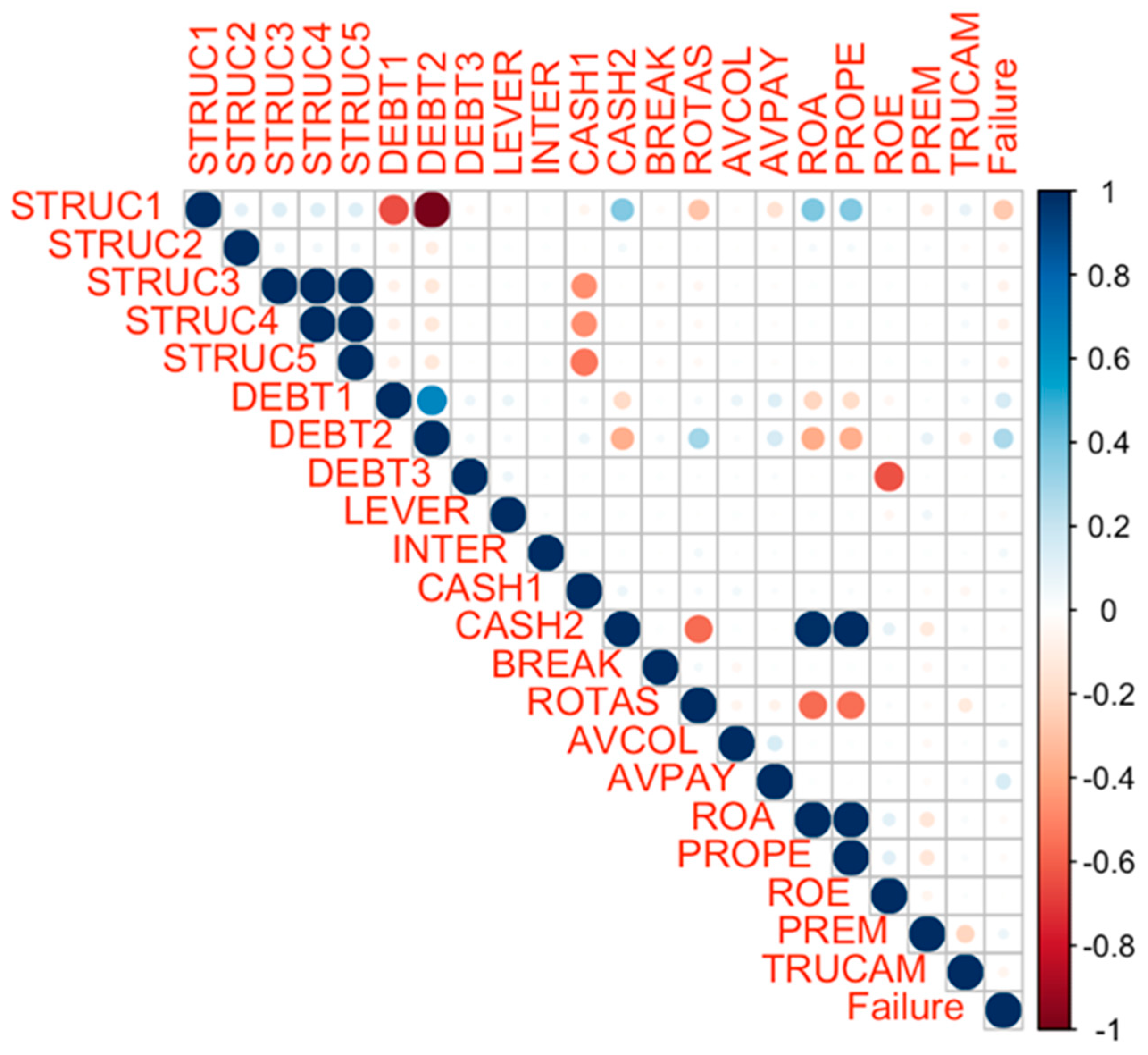
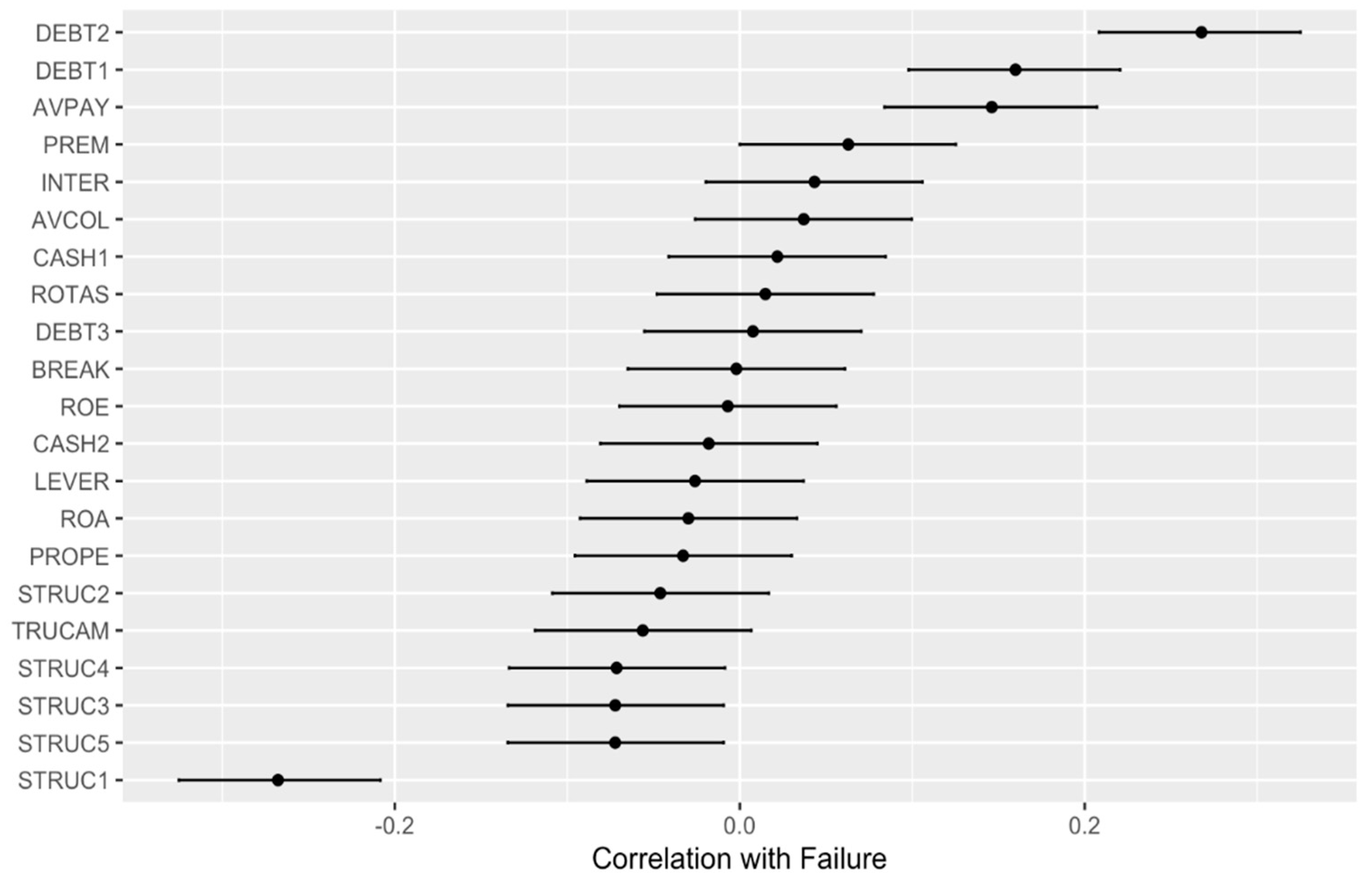
4.1. Analysis of Correlations

To identify high correlations among predictors and the response variable, we created a correlation plot or correlogram (Figure 1). The plot reveals that only a small number of variables exhibit strong correlations, highlighted by larger points and more intense colors. A correlogram visually represents the correlation matrix, where each coefficient is depicted using color and point size based on its value. The analysis shows some correlations among variables related to structure, indebtedness, and profitability. However, the XGBoost machine learning algorithm effectively handles correlated independent variables, as supported by previous studies [51,52,53]:
XGBoost includes integrated regularization mechanisms that penalize model complexity, reducing the impact of variable correlations. It prunes decision tree branches that do not provide significant information, minimizing the overload caused by correlations.
XGBoost emphasizes identifying nonlinear interactions between variables rather than solely considering their individual effects. This approach allows the algorithm to leverage the information contained in correlations without being adversely affected by their presence.
XGBoost has proven to be robust in handling multicollinearity, i.e., high correlations among independent variables. Multiple studies have shown that its performance remains largely unaffected in such scenarios.
In summary, XGBoost is a robust algorithm against multicollinearity, meaning its performance remains largely unaffected by the presence of high correlations among independent variables [40].
Additionally, Figure 2 illustrates the correlations (and 95% confidence intervals) between all predictors or variables and the propensity to fail (Failure, the term used for the financial strength indicator VADIS 2PBB) in the dataset. This analysis suggests that Failure has a relatively positive correlation with certain debt-related variables and the variable AVPAY (average payment period in days), indicating that increases in these variables are associated with a higher likelihood of failure. Conversely, there is a noticeable negative correlation with variables linked to financial structure, particularly with the variable STRUC1 (solvency ratio), suggesting that decreases in these variables are associated with an increased propensity to fail. These findings are further reflected in Figure 3, which highlights the ten independent variables most strongly correlated with the dependent variable, propensity to fail—negative correlations are shown in red, while positive correlations are depicted in blue.

4.2. Descriptive Analysis

Table 3 presents the main descriptive statistics for the data analyzed in the study of societies’ propensity to fail. The table includes the ten independent variables most strongly correlated with the Failure variable. These statistics provide essential information about the variables, including their central tendency, variability, and overall distribution. It is important to note that the variables representing ratios are expressed as percentages.
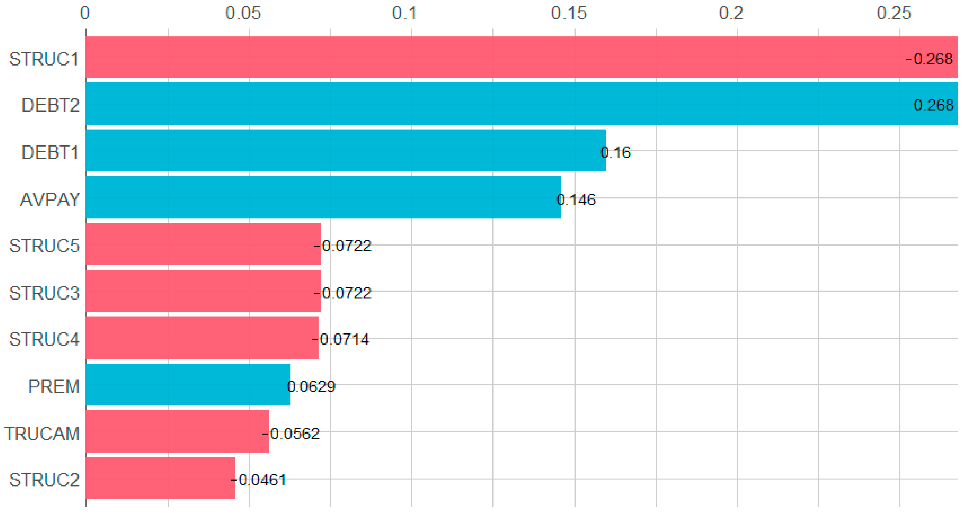
  • STRUC1 (Solvency Ratio): the solvency ratio reflects a company’s ability to meet its short-term obligations relative to its adjusted net equity. With a median of 45.33 and a standard deviation of 40.75, there is considerable variability in this indicator among the companies.
  • DEBT2 (Indebtedness): this metric measures the proportion of assets financed by debt relative to total assets. With a median of 54.67 and a standard deviation of 40.75, a significant variability is evident in the level of indebtedness among the companies.
  • DEBT1 (Total Debt Percentage Ratio): This ratio assesses a company’s level of indebtedness relative to its net equity and total liabilities. With a median of 17.34 and a standard deviation of 30.62, a moderate level of variability in indebtedness is observed across the companies.
  • AVPAY (Average Payment Period): this variable indicates the average time a company takes to settle its trade debts. The high standard deviation of 247.13 highlights considerable variability in payment periods among the companies.
  • STRUC5 (Immediate Liquidity Ratio): this ratio measures a company’s ability to cover its short-term liabilities with its most liquid assets. With a median of 49.91 and a staggering standard deviation of 5480.31, the indicator reveals extreme variability, suggesting significant differences in immediate liquidity among the companies.
  • STRUC3 (General Liquidity Ratio): this metric assesses the company’s ability to meet short-term liabilities with its current assets. A median of 157.18 and a standard deviation of 6636.64 indicate substantial variability in general liquidity across the sample.
  • STRUC4 (Acid Test Ratio): this ratio provides a stricter measure of liquidity by excluding inventory from current assets. With a median of 123 and a high standard deviation of 6603, there is considerable variability in companies’ ability to cover short-term liabilities without relying on inventory.
  • PREM (Worker Costs/Operating Income): This metric measures the proportion of labor costs relative to operating income. A median of 17.69 and a standard deviation of 27.78 indicate moderate variability in this ratio across the sample.
  • TRUCAM (Environmental Risk Score): this score evaluates the environmental risk faced by companies. With a median of 3.16 and a standard deviation of 21.60, the data shows moderate variability in environmental risk scores across the sample.
  • STRUC2 (Solidity Ratio): this ratio assesses a company’s ability to meet long-term liabilities based on its net equity and non-current assets. The median of 104 indicates a relatively low level of solidity on average, though the extremely high standard deviation of 16,570.81 reflects significant dispersion in the data.
  • Failure (Propensity to Fail, VADIS 2PBB): this indicator represents the likelihood of business failure. With a median of 3 and a standard deviation of 1.44, there is some variability in failure rates in the data

4.3. Data Analysis

After completing the descriptive analysis, and to provide greater rigor to the findings, we will conduct a detailed analysis using machine learning tools. This approach will allow us to assess the relevance of the variables considered in explaining the propensity for business failure.

4.3.1. Applied Methodology

Using a set of accounting and financial predictors, we aim to build a reliable regression model capable of predicting the propensity to fail among enterprises. Additionally, the model seeks to identify the variables with the greatest impact on this propensity. Our goal is to develop a predictive model and validate its performance on a hypothetical sample different from the training dataset, leveraging machine learning techniques. The algorithm used is XGBoost, a member of the gradient boosting family, chosen for its excellent performance in regression contexts. Boosting-based models are characterized by their adaptive integration of a large number of relatively simple decision tree models. This approach produces highly accurate combined predictions, significantly outperforming the individual decision trees that make up the final combined model [27].
This technique can be applied in both classification and regression contexts, often providing much better results than those obtained with more traditional statistical methods, such as Ordinary Least Squares or logistic regression. Its success lies in the sequential combination of many simple models (or “weak learners”) by boosting algorithms. These models collectively produce highly accurate predictions, which are essentially an average of the predictions made by all the combined simple models. As highlighted by James et al. [54], this approach results in predictions characterized by very low variance, ensuring highly reliable outcomes. This reliability, combined with the adaptability of boosting techniques, makes XGBoost a powerful tool for predictive analysis in various contexts, including the study of enterprises’ propensity to fail.
Chen and Guestrin [40] describe XGBoost as a scalable and effective implementation of the gradient boosting technique originally developed by Friedman [51] and Friedman et al. [55]. Decision trees in XGBoost are built sequentially, with each tree leveraging information from previously generated trees to correct errors carried over. Each tree is fitted to a modified version of the original dataset, which has been adjusted based on the residual errors yet to be addressed. Consequently, the construction of each tree heavily depends on the trees already built [56]. As James et al. [54] point out, the algorithm refines the model at each iteration by fitting a new tree to the current residuals rather than the dependent variable’s values. The algorithm then integrates this new tree into the adjusted model to update the residuals, progressively improving the model’s predictive accuracy. In summary, XGBoost continues adding new trees until no further improvement in predictive performance is achievable. Each sequential model aims to correct the errors of the preceding model, with the accuracy of the final model being the cumulative result of this iterative error-correction process.
The XGBoost algorithm generates a set of simple models based on decision trees, where the inclusion of each additional tree significantly enhances the predictive capacity compared to individual decision trees within the ensemble. Another important feature of the XGBoost model is its incorporation of regularization during the decision tree construction process. Regularization, a key concept in machine learning, serves as a mechanism to control the weight assigned to variables in the final model. This feature distinguishes XGBoost from other gradient-boosting-based algorithms and significantly reduces the likelihood of developing models that fail to generalize effectively to independent datasets. This capability ensures that the resulting model is not only accurate but also robust and applicable to a broader range of data scenarios.
The fact that XGBoost is composed of an ensemble of decision trees, with predictions derived from the combined output of these trees, allows it to overcome the limitations of individual decision trees, which are typically characterized by poor predictive performance. Climent et al. [33] and Carmona et al. [41] applied this methodology using classification trees to predict banking failure in the Eurozone and the U.S., respectively. However, this study applies the XGBoost technique utilizing regression trees, adapting the method to the specific objective of predicting the propensity to fail among enterprises. This approach leverages the strengths of XGBoost, particularly its ability to enhance accuracy and generalizability while addressing the limitations of single-tree models.

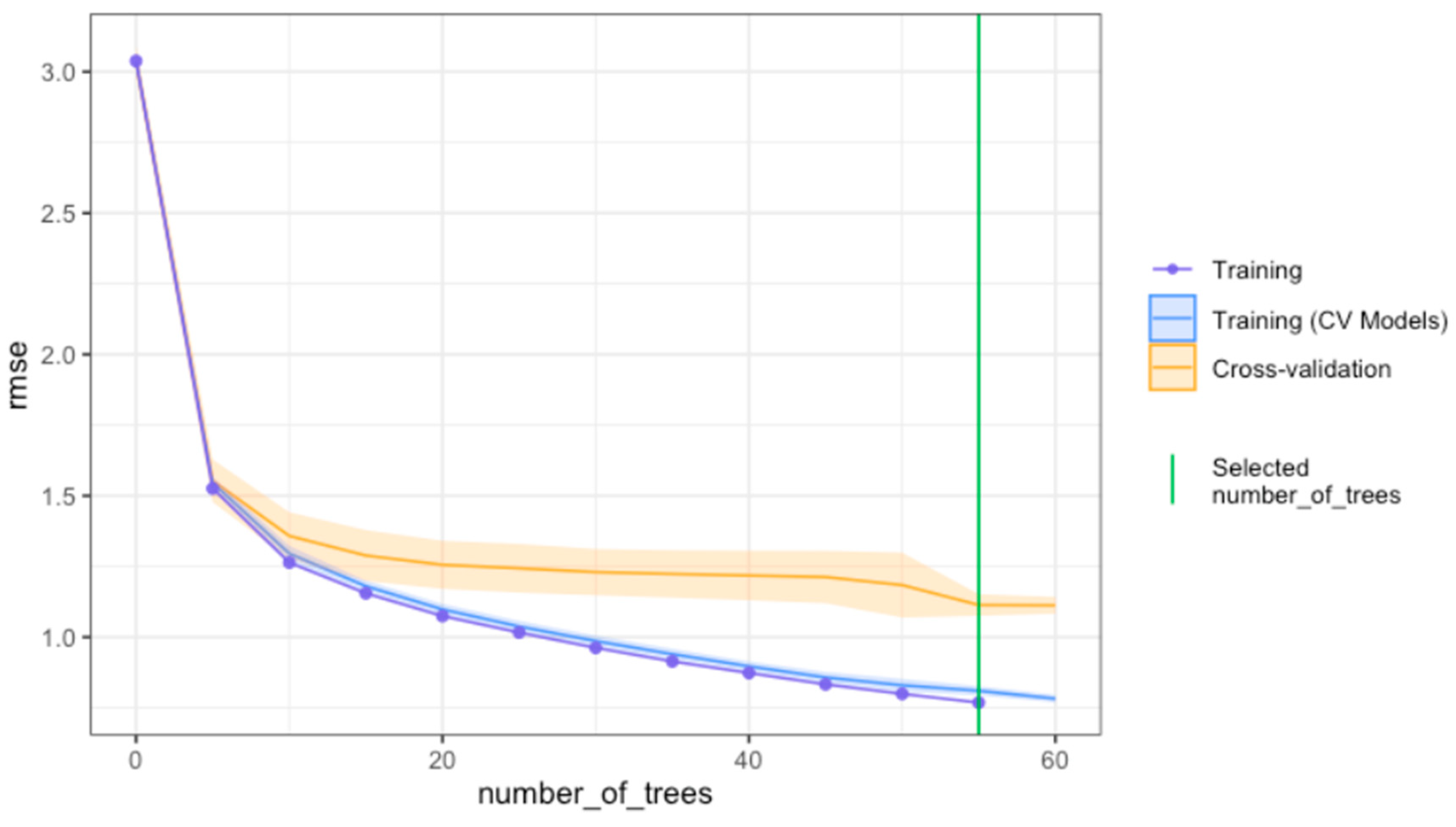
4.3.2. Procedure for Tuning the XGBoost Model

The initial sample of 971 enterprises was divided into two subsamples: a training set and a validation set. The training set consists of a random selection of 75% of all observations, while the validation set comprises the remaining 25%. The training sample is used to fit a robust regression model based on the XGBoost algorithm, and the validation sample is employed to evaluate the results obtained from the training process. The validation sample remains hidden from the algorithm throughout the entire training process, ensuring that the XGBoost model is not influenced by the characteristics of the validation data. This approach enables the development of highly generalizable models with strong predictive capabilities when applied to new, unseen data. It is crucial to understand that powerful machine learning algorithms like XGBoost have the potential to memorize the training data. Therefore, ensuring the robustness and validity of the model requires the use of independent samples, such as the validation set. In summary, 25% of the observations were allocated to validate the goodness-of-fit or internal validation of the model on an independent sample. This allows us to confidently assert that the results obtained are generalizable to new data.
Obtaining the best XGBoost model for the available dataset requires identifying the optimal values for its hyperparameters, including the optimal number of decision trees. This involves an iterative process that tests various combinations of hyperparameter values to identify the best configuration. The primary goal is to find the combination that maximizes the model’s predictive capacity while avoiding overfitting or underfitting (to explore in greater depth the set of hyperparameters that influence the learning process of the XGBoost algorithm, please refer to [57]).
To fit an XGBoost regression model with an optimal combination of hyperparameters, the process utilized the cross-validation technique. Specifically, for each hyperparameter combination, the approach implemented 10-fold cross-validation (k = 10). The procedure involved training 10 models, each using a different subset containing 90% of the observations, while reserving the remaining 10% for validation. The evaluation of the model’s performance relied on averaging the results across all 10 validation subsets. This method ensures robust performance metrics by minimizing dependence on any single partition of the dataset, providing a reliable measure of the model’s predictive accuracy and generalizability.
After completing the cross-validation process for each combination of hyperparameters, the process estimates an additional model using 100% of the observations. This final model represents the outcome for that particular hyperparameter combination. As a result, the process estimates a total of 11 models for each combination of hyperparameters (k + 1 = 10 + 1), generating both internal performance metrics for the final model and those from cross-validation. The total number of models grows with the number of hyperparameter combinations. Given that 50 combinations were considered, the process estimated a total of 550 models (11 × 50) to identify the model with the highest predictive capacity. This comprehensive approach ensures that the selected model is optimized for accuracy and generalizability.
Additionally, to identify an effective combination of hyperparameters that produces a robust and highly predictive model, the process used a technique known as random search within the space of all possible hyperparameter combinations. Specifically, 50 random combinations were selected from the search space, representing a subset of all potential configurations.
In summary, cross-validation enables the identification of an optimal hyperparameter combination, ensuring the development of a robust and highly generalizable XGBoost regression model. This approach balances computational efficiency with the precision needed for accurate model tuning.
Figure 4 visually illustrates the model adjustment process, showing that the optimal XGBoost model—corresponding to the lowest possible value of RMSE (root mean squared error)—in cross-validation samples is achieved with approximately 55 decision trees. Beyond this number of trees, a slight deterioration in the RMSE is observed in the cross-validation samples, although the training sample shows improvement. As expected, cross-validation results are worse than those from the training sample. Consequently, the ideal number of decision trees for model tuning is 55. Based on the analysis, there is no evidence of overfitting, and the model can be confidently applied to independent samples.
Once a suitable XGBoost model has been identified based on the sample’s characteristics, the independent validation sample (25% of the total observations) is used to calculate goodness-of-fit performance metrics. It is crucial to emphasize that these metrics are derived from the validation sample, offering a more conservative assessment than those obtained from the final model trained on the training sample. Relying solely on performance metrics from the training sample is a flawed practice when working with complex and powerful algorithms like XGBoost. These algorithms can memorize portions of the training data during the learning process, leading to overly optimistic results and the risk of overfitting. By using an independent validation sample, the evaluation provides a more realistic measure of the model’s predictive performance and generalizability, ensuring its robustness when applied to new, unseen data.
To implement the XGBoost algorithm, the statistical programming environment R (version 4.4.0) [58] and the h2o library (version 3.44.0.3) [59] were used. This statistical programming platform was employed to demonstrate the potential of these techniques in analyzing the propensity to fail among companies in the sample.

4.3.3. Model Performance of the Fitted XGBoost Model

We constructed an XGBoost model incorporating all the variables listed in Table 3, following the described methodology. The primary objective was to identify the most relevant variables for determining the propensity to fail in societies. As is usual in regression scenarios within machine learning, we used the RMSE (root mean squared error) performance indicator to identify the best-fitted model based on the various hyperparameter combinations considered. This approach ensures the selection of a model with high predictive accuracy while maintaining robustness and generalizability.
As previously mentioned, 50 primary XGBoost models were constructed, each corresponding to a different combination of hyperparameters, along with their respective cross-validation models. The final model was selected based on the best RMSE value achieved during the hyperparameter optimization process. The RMSE for the selected model was 1.21 on the 10-fold cross-validation and 1.31 on the independent validation sample. Since the difference between these two values is small, the resulting model does not exhibit overfitting and is generalizable when applied to independent data or new samples. This confirms the robustness and reliability of the model for predicting the propensity to fail among considered societies.
Figure 5 displays the distribution of residuals obtained in the independent validation sample—the difference between predicted and actual values—for the adjusted XGBoost model, represented through a box plot. The residual distribution is relatively narrow, reflecting the effectiveness of the resulting XGBoost model. The red dot on the plot indicates the root mean squared error (RMSE) of the adjusted model. The residuals in the validation sample show a median below 1.5 and a mean below 1, demonstrating the model’s accuracy and its ability to provide reliable predictions.
To complete the evaluation of the model performance, Table 4 presents the RMSE values for the training sample, the cross-validation samples, and the validation sample (the latter corresponding to the red dot depicted in Figure 5).
Table 4 provides a clear comparison of the model’s performance across different data subsets, highlighting its robustness and consistency. The alignment of RMSE values across the cross-validation samples and the validation sample further supports the absence of overfitting and demonstrates the model’s reliability in making predictions on new, unseen data.
In the training sample, all observations from the database are included, and the error is calculated based on these data. In this case, the data used to compute the performance metrics matches the data used to train the model. As a result, these outcomes are often overly optimistic and should not be used as a reference. The cross-validation samples are employed to identify the hyperparameters that yield a well-performing model. Meanwhile, the validation sample provides the final estimate of the model’s performance on independent data that were not used during model fitting or training. These results are more conservative yet realistic and should be the primary reference for evaluating the performance of the adjusted models.
It is worth noting that in many machine learning algorithms, the differences between the results from the training sample and those from cross-validation and validation samples are often significant because the former tends to be overly optimistic and does not accurately reflect the performance on an independent sample. As previously mentioned, relying on performance metrics obtained from the training sample is not good practice, as they tend to overestimate the model’s accuracy. However, in this case, the XGBoost model demonstrates low error rates across the training, cross-validation, and validation samples. This consistency in performance underscores the goodness-of-fit and reliability of the model, even when evaluated on independent data.

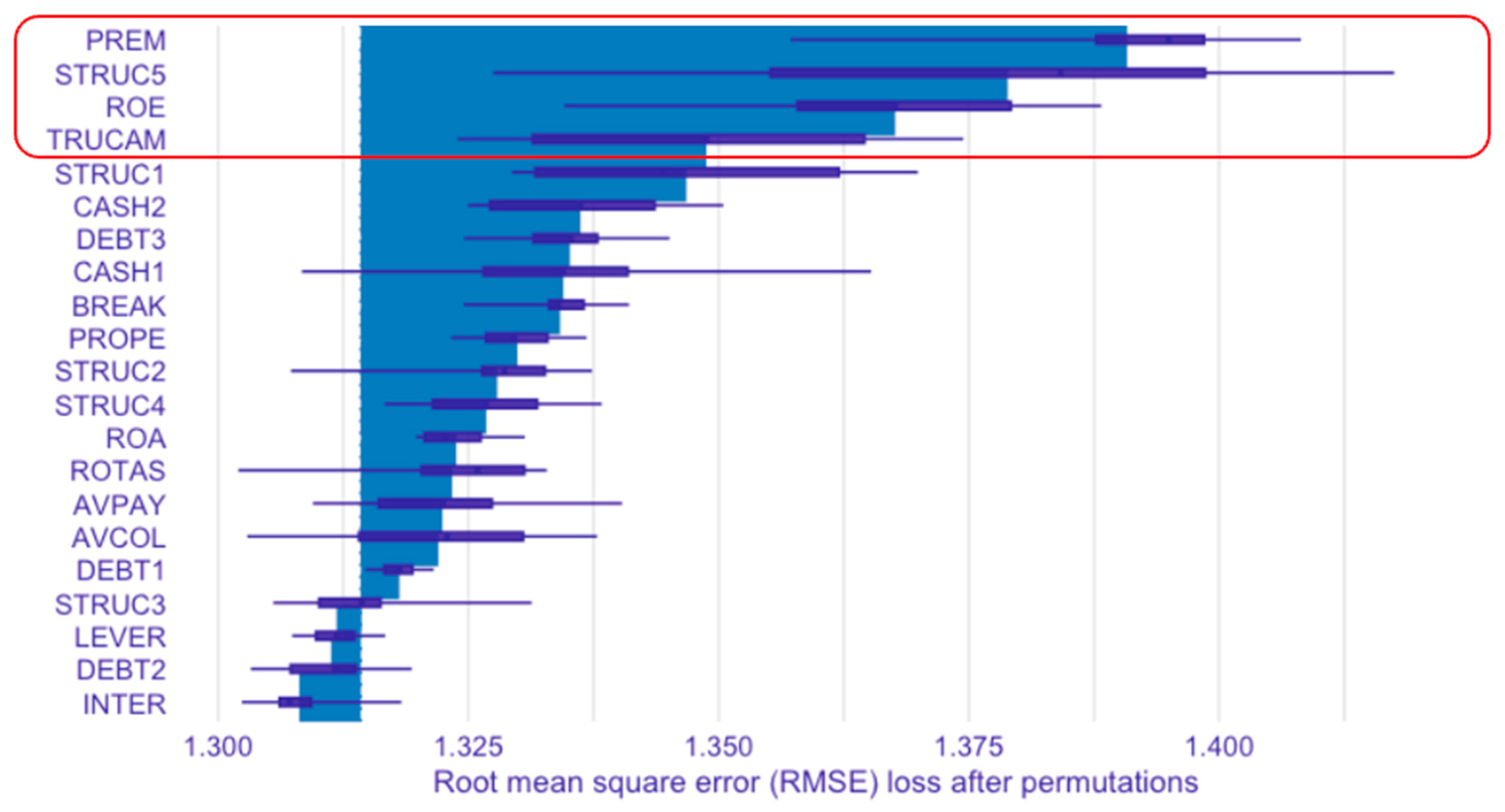
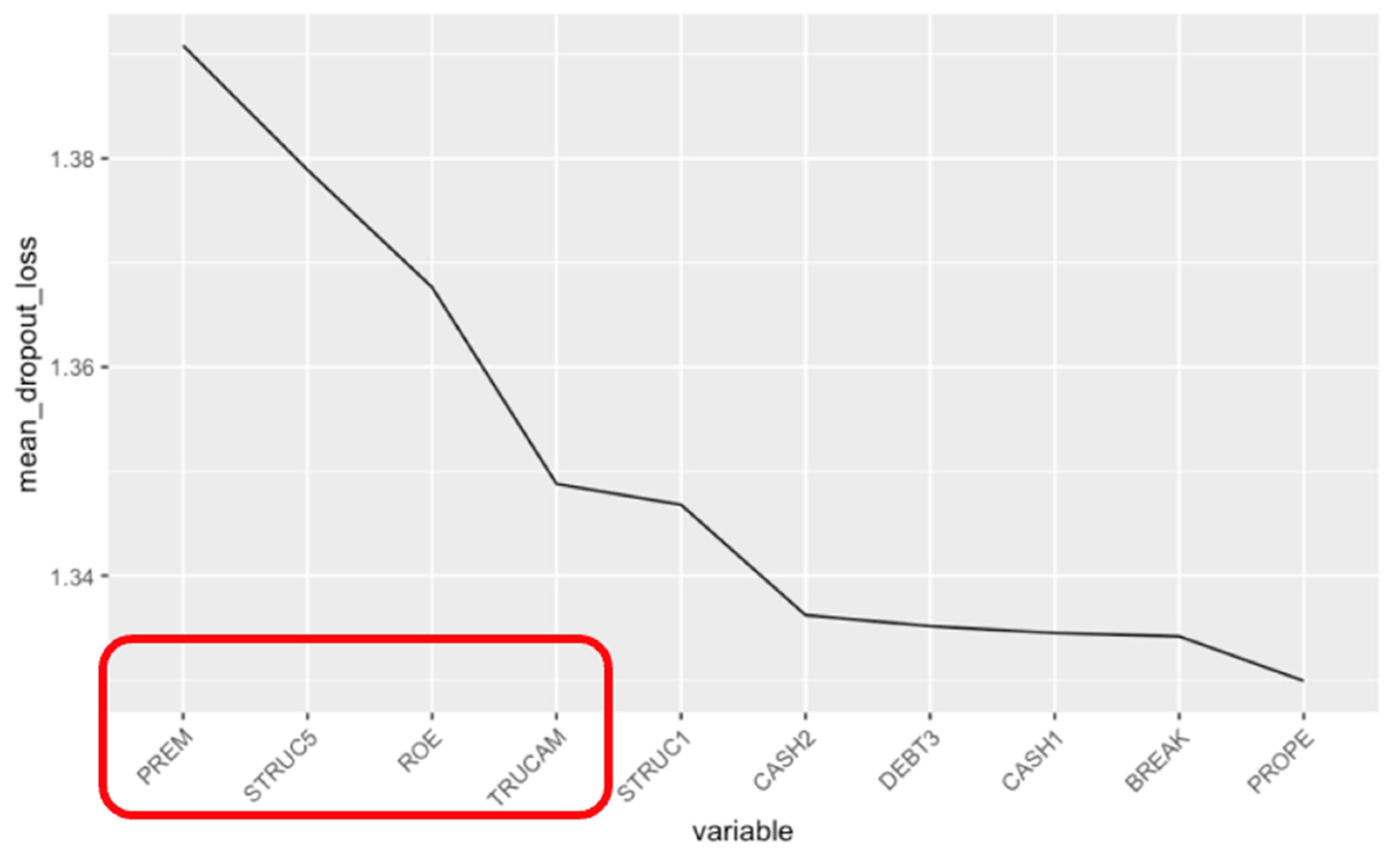
4.3.4. Most Relevant Variables in the XGBoost Model

Figure 6 and Figure 7 illustrate the importance of the most relevant variables in relation to the dependent variable (propensity to fail), as identified by the XGBoost algorithm.
Key observations include the following:
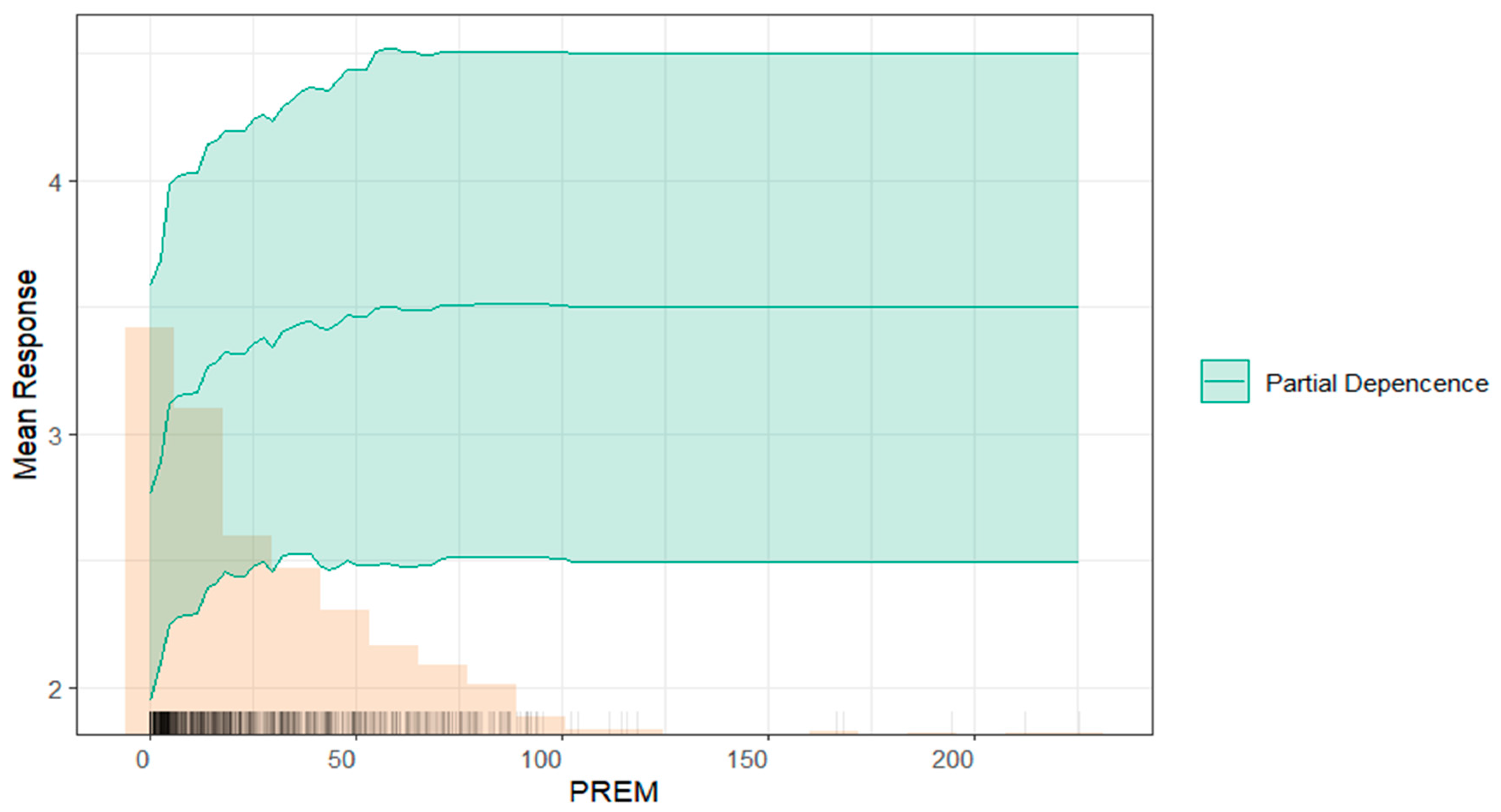
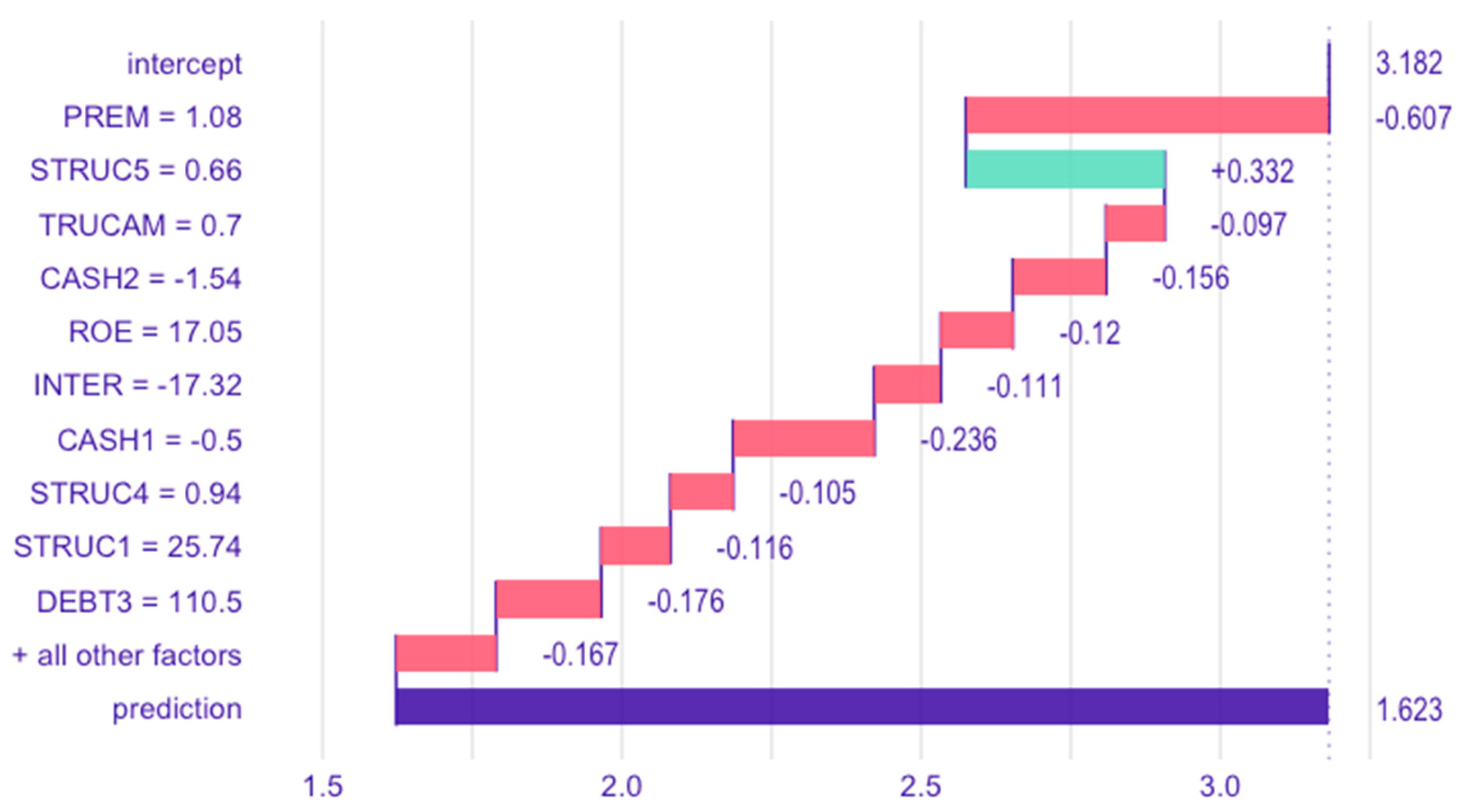
  • PREM (Worker Costs/Operating Income): this variable stands out as the most significant predictor, highlighting the critical role of labor cost efficiency in determining the financial stability of companies in the sample;
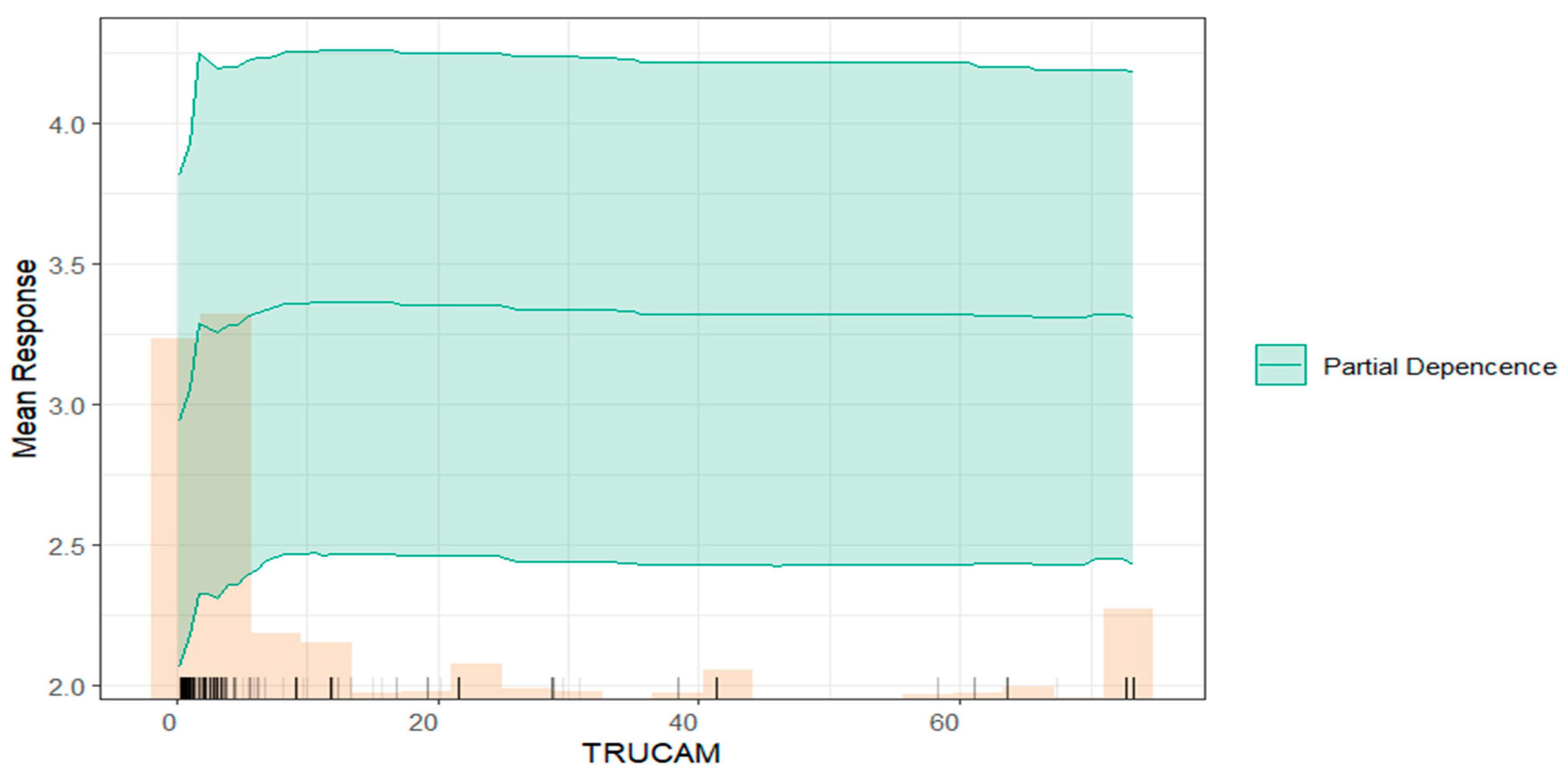
  • TRUCAM (Environmental Risk Score): ranked among the top four variables, TRUCAM underscores the relevance of environmental risk and their impact on the organization. This finding emphasizes the need for effective environmental risk management to ensure sustainability among the sample of companies.
These insights provide a deeper understanding of the drivers of failure propensity and highlight the interplay between financial, operational, and environmental factors in business viability.
Next, we will represent and analyze graphically the relationship between the propensity to fail among the sample of companies and the four most relevant independent variables. For this purpose, we will use partial dependence plots generated from the XGBoost model.
These plots illustrate the marginal effect of each variable on the prediction of failure propensity when considered independently. The x-axis represents the range of values each variable can take, while the y-axis shows the predicted propensity to fail. Partial dependence plots can reveal whether the relationship between the dependent variable and a predictor is linear or more complex.
The estimation of these relationships is derived from the training data using techniques such as the Monte Carlo method. Partial dependence plots provide a global perspective, as they consider all observations and depict the overall relationship between a variable and the dependent variable predictions produced by the model [60].
This analysis will deepen our understanding of how the most influential variables—such as PREM and TRUCAM—affect the likelihood of failure, offering actionable insights for improving business resilience.
According to Figure 8, there is a positive relationship between the propensity to fail and the variable PREM (worker costs divided by operating income). The line slopes upwards, suggesting that higher values of PREM are associated with a higher predicted probability of failure. This indicates the negative effect that worker costs exert on a company’s continuity risk.
In Figure 9, we observe that within the range where most observations are concentrated, a decrease in the variable STRUCT5 (immediate liquidity ratio) leads to an increase in the estimated propensity to fail for the companies analyzed.
In Figure 10, a negative relationship is evident between the propensity to fail among societies and the variable ROE (financial profitability). This indicates that higher financial profitability reduces the likelihood of failure.
Regarding the variable related to environmental risk (TRUCAM), Figure 11 shows that within the range where observations are most concentrated, an increase in TRUCAM corresponds to a higher propensity to fail.
We understand that the relationship between environmental risk and the propensity to fail is not straightforward and depends on various factors such as the sector of activity, company size, and geographic location. However, environmental financial exposure can increase operational expenses, potentially making companies less competitive and more vulnerable to failure. Additionally, companies incurring significant environmental risk may face regulatory penalties or legal actions, further contributing to the risk of failure.

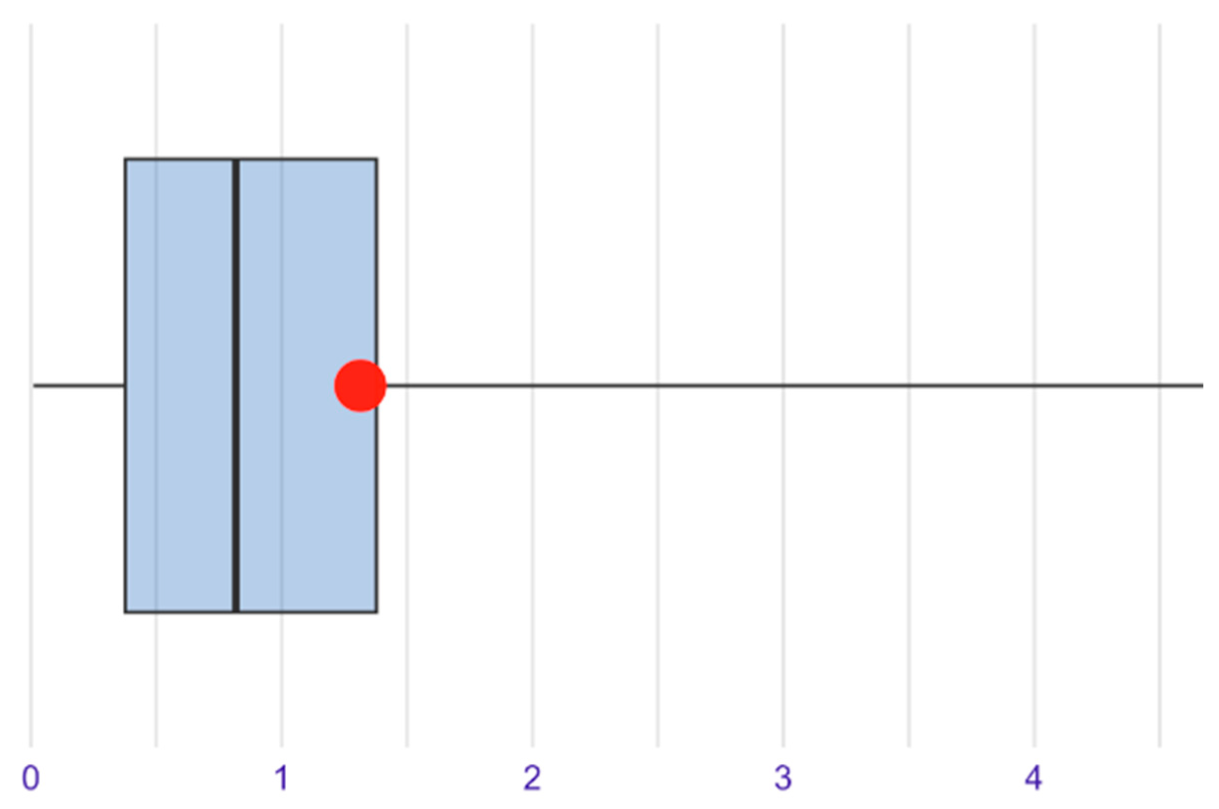
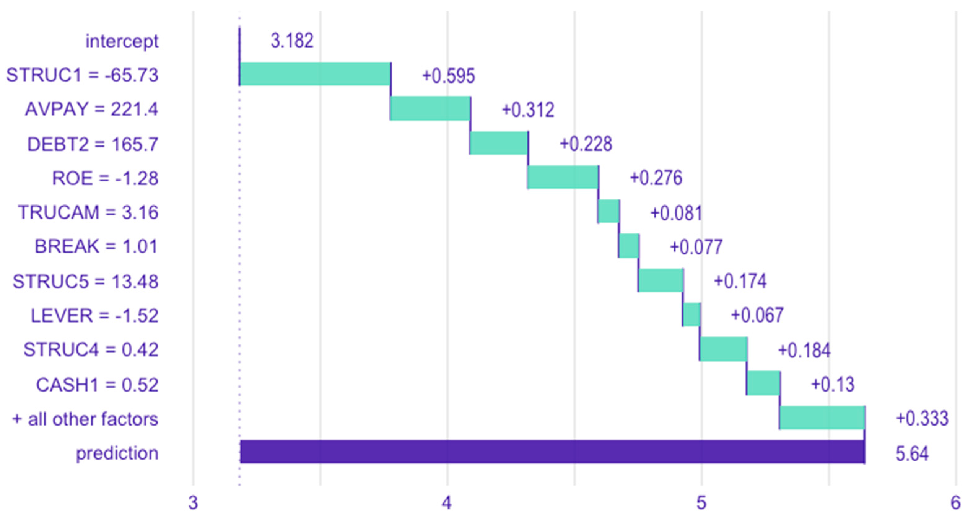
4.3.5. Effect of Variables on Model Predictions at the Individual Observation Level

Finally, we will demonstrate how it is possible to interpret the XGBoost model at a level that reveals the effect of each variable on individual observations. To illustrate this, we will consider one observation where the model assigns a high propensity for business failure (Figure 12) and, conversely, an observation with a very low propensity to fail (Figure 13). This analysis allows us to pinpoint which variables are driving the predictions in both scenarios.
These representations fall within what is known as the local interpretation of a model, helping to understand a machine learning model and its predictions for individual observations [61]. In this regard, it is highly valuable, and sometimes even necessary, to evaluate the effect of independent variables on the predictions a model provides for a specific observation. In this study, a researcher or financial analyst might be interested in understanding why the XGBoost algorithm assigns high propensity-to-fail scores to a particular company, based on the values of the independent variables for that company. This approach demonstrates that individual predictions are fully transparent, addressing the limitations of these complex algorithms, which are sometimes criticized for being “black boxes”.
Consequently, to demonstrate the transparency of the XGBoost model, it is valuable to identify which variables have the greatest influence on the prediction for any given company. This involves calculating the contribution of the independent variables that carry the most weight in these individual predictions [41,62].
In machine learning, the so-called break down plots provide a straightforward way to summarize the effect of each predictor on the model’s dependent variable. For a specific observation, the probability that a company is prone to failure is decomposed into the individual impacts of each variable in the model. The previously mentioned Figure 12 and Figure 13 contain these break down plots, illustrating the contributions of the independent variables to the predicted propensity to fail for two distinct cases.
In these figures, it is evident that the base model (Intercept) assigns a general propensity-to-fail score of 3.182, which is calculated without considering the predictive capacity of the individual variables. This value represents the average prediction for the propensity to fail made by the XGBoost model. For instance, in the case of the company shown in Figure 12, the predicted propensity-to-fail score is 5.64. This prediction can be decomposed to reflect the influence of the most relevant variables as follows:
+3.182: Base model (Intercept);
+0.595: STRUCT1 = −65.73 [now the prediction is 3.777];
+0.312: AVPAY = 221.4 [now the prediction is 4.089];
+0.228: DEBT2 = 165.7 [now the prediction is 4.317];
+0.276: ROE = −1.28 [now the prediction is 4.593];
+0.081: TRUCAM = 3.16 [now the prediction is 4.674];
+0.077: BREAK = 1.01 [now the prediction is 4.751];
+0.174: STRUC5 = 13.48 [now the prediction is 4.925];
+0.067: LEVER = −1.52 [now the prediction is 4.992];
+0.184: STRUC4 = 0.42 [now the prediction is 5.176];
+0.130: CASH1 = 0.52 [now the prediction is 5.306];
+0.333: Rest of variables [final prediction is 5.64].
In these prediction plots, it can be observed that high values of the variable related to environmental risk (TRUCAM) push the prediction model to assign higher values to the propensity-to-fail prediction for a company. Conversely, low values of the TRUCAM variable contribute to producing very low predictions for the propensity to fail.

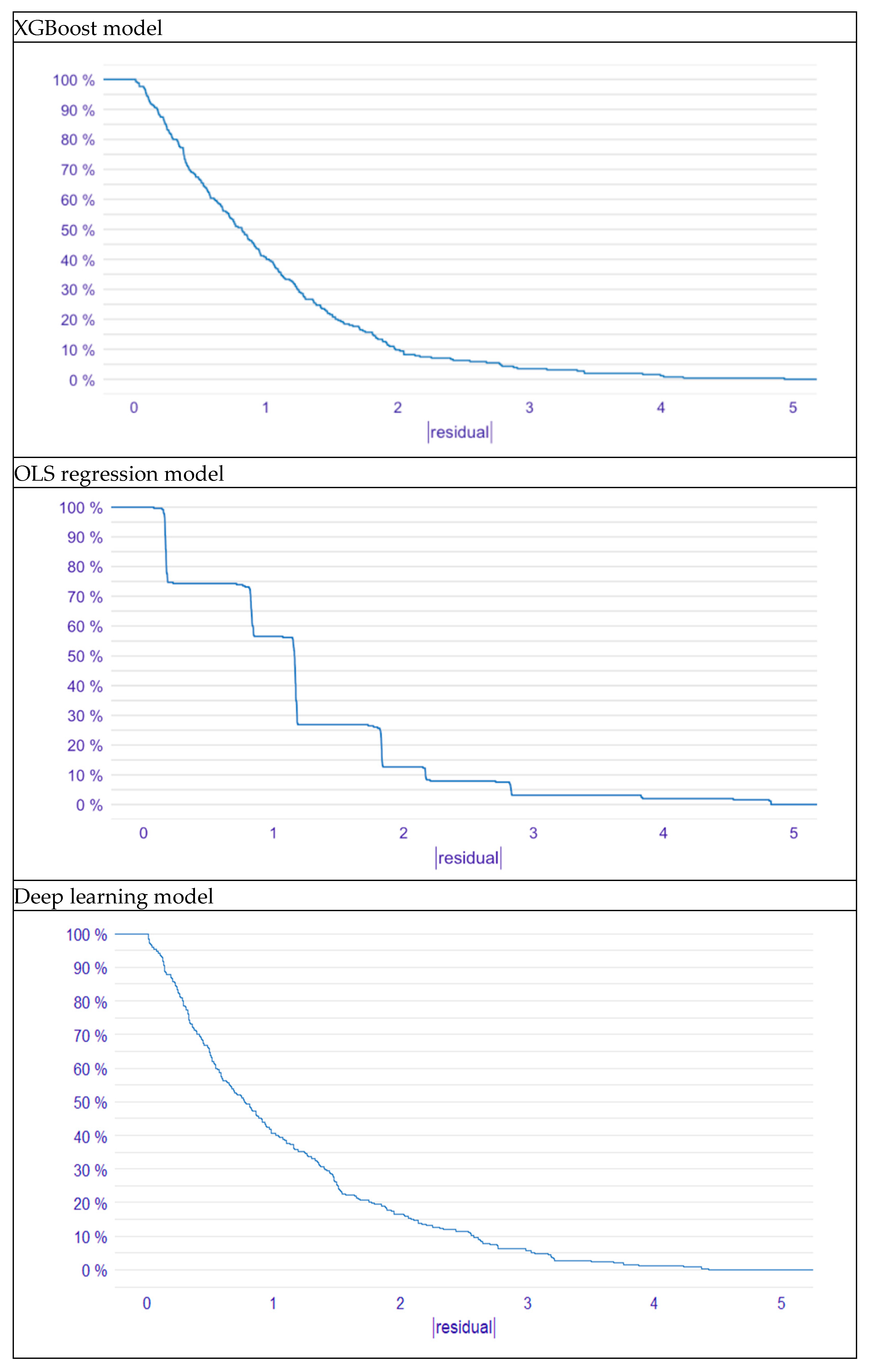
5. A Comparison of XGBoost with Two Other Classification Models

After developing a predictive model for business failure using the XGBoost algorithm, which demonstrated strong performance, we conduct a comparative analysis. This analysis contrasts two methodologies: a traditional Ordinary Least Squares (OLS) regression model and a modern deep learning model. OLS regression is a standard statistical method used to analyze linear relationships. In contrast, deep learning is a sophisticated machine learning technique capable of capturing intricate patterns within data. This comparison aims to explain the relative advantages and disadvantages of each approach when applied to the prediction of business failure.
Ordinary Least Squares (OLS) regression, commonly referred to as linear regression, is a traditional statistical technique used to model the linear relationship between a dependent variable and one or more independent variables. The core principle of OLS regression is to minimize the sum of squared residuals, which represent the differences between the observed values and the values predicted by the model. The OLS model is formally represented by the following equation:
Y = β0 + β1X1 + β2X2 + … + βpXp + ϵ
where
  • Y denotes the dependent variable.
  • β0 represents the intercept of the regression line.
  • β1, β2, …, βp are the coefficients corresponding to the independent variables X1, X2, …, Xp, respectively. These coefficients quantify the change in the dependent variable associated with a one-unit change in the corresponding independent variable, holding all other variables constant.
  • ϵ indicates the error term, which accounts for the unexplained variance in the dependent variable.
The OLS estimation procedure involves calculating the coefficient values (β) that minimize the sum of the squared residuals. After these coefficients are estimated, the model can be employed to predict the value of the dependent variable for new observations, given the values of their independent variables.
In contrast to traditional statistical methods, deep learning, a subfield of machine learning, utilizes artificial neural networks with multiple layers (often referred to as “deep” networks) to determine complex patterns and hierarchical representations within data [63]. A key distinction of deep learning is its capacity for automated feature extraction, reducing the need for manual feature engineering that is often required in conventional models [64].
The fundamental building block of a deep learning model is the artificial neuron. Each neuron receives inputs, processes them using learnable weights and biases, and produces an output through an activation function. These neurons are organized into interconnected layers, forming a layered architecture (as depicted in Figure 14). The network typically consists of an input layer, which receives the raw data; multiple hidden layers, which successively refine the information via nonlinear transformations; and an output layer, which provides the final prediction (e.g., predicting business failure returns in a financial context). This layered structure allows the model to learn intricate relationships within datasets, including nonlinear interactions between independent variables, which are often prevalent in financial data.
Deep learning models, such as the multi-layer feedforward neural networks illustrated in Figure 15, require substantial training datasets and utilize backpropagation algorithms to iteratively refine the network’s parameters (weights and biases). The objective of these adjustments is to optimize the model’s accuracy by minimizing the difference between predicted and actual outcomes [63]. Within these architectures, each connection between an input and a neuron has an associated learnable weight (represented as w1, w2, …, wn). These weights are crucial parameters that are adjusted during the training process to improve the model’s predictive capabilities.
The transmission of signals between layers in a neural network is controlled by activation functions [65]. These functions introduce nonlinear transformations to the weighted sum of inputs, enabling the network to model complex, nonlinear relationships often found in financial data. Examples of such relationships include interactions between market volatility, leverage ratios, and operational efficiency. The input layer receives raw financial data (e.g., historical prices, financial ratios). The hidden layers then progressively refine feature representations through successive transformations, extracting increasingly abstract and relevant features. Finally, the output layer produces the model’s predictions, such as estimated mutual fund returns.
This iterative optimization process, driven by backpropagation and large datasets, empowers deep learning models to automatically discover nonlinear associations and hierarchical patterns within data. This capability often allows them to exceed the performance of linear methods like OLS regression, which are inherently limited in capturing such complexities. For a more comprehensive understanding of neural network architectures, training procedures, and their applications in financial analytics, readers are referred to Romero et al. [66].
Deep learning models present significant advantages in the context of business failure prediction, primarily due to their capacity to handle high-dimensional datasets and model nonlinear interactions between variables [67]. These characteristics make them a compelling alternative to traditional methods like OLS regression, which relies on the assumption of linearity and may, therefore, fail to capture complex patterns present in financial data.
For this investigation, a deep neural network specifically designed for regression tasks is employed. The network architecture incorporates multiple hidden layers, each utilizing nonlinear activation functions (such as ReLU or sigmoid). This design enables the model to learn intricate, hierarchical relationships within the business failure data, including the complex interaction between various independent variables. Through the iterative process of backpropagation, the network refines these learned representations, adapting to capture the factors that contribute to business failure. This adaptive learning process is expected to result in improved prediction accuracy compared to linear approaches.
This part of the study assesses the efficacy of the XGBoost algorithm for predicting business failure by comparing its performance to two established benchmark models: OLS regression and deep learning architecture. Table 5 summarizes the key performance metrics for all three models, evaluated on the test dataset. These metrics include Mean Squared Error (MSE), Root Mean Squared Error (RMSE), Mean Absolute Error (MAE), and mean residual deviance. The baseline XGBoost results are also included in the table. The results demonstrate that the XGBoost model achieves superior performance compared to both the OLS regression and deep learning models across all reported metrics.
Figure 16 presents the reverse cumulative distribution of absolute prediction errors for the XGBoost, OLS regression, and deep learning models, evaluated using validation data. This visualization provides a detailed comparison of the error magnitudes across the different models. A smaller area under the curve in this plot signifies better predictive accuracy, as it indicates a higher concentration of predictions with low absolute errors. The XGBoost model exhibits the smallest area under the curve, confirming its superior performance in minimizing prediction errors. This suggests that XGBoost more effectively captures the underlying relationships between the predictor variables and business failure compared to the OLS regression and deep learning models. From the XGBoost plot, several conclusions can be drawn, indicating a low incidence of large prediction errors.
  • The model exhibits very few errors exceeding a magnitude of 2, accounting for less than 10% of the total residuals.
  • Errors greater than 3 constitute less than 5% of the total in the XGBoost model.
In summary, this analysis of residuals in the validation sample confirms the strong predictive performance of the XGBoost model.

6. Discussion

6.1. Interpretation of Significant Results

The study identifies environmental risk as a significant predictor of business failure, using the XGBoost machine learning algorithm. This finding aligns with previous research emphasizing the importance of sustainability in business operations [5,9,37]. However, the study diverges from traditional models by incorporating environmental risk as a primary variable, which is relatively novel in the context of business failure prediction.
The positive correlation between environmental risk (TRUCAM) and the propensity to fail suggests that higher environmental risk increases the likelihood of business failure. This result is consistent with the notion that environmental financial exposure can reduce profitability and, consequently, affect a company’s viability. The study also finds that labor costs (PREM), liquidity (STRUC5), and financial profitability (ROE) are significant predictors, which is in line with traditional financial distress models [1,3]. Moreover, the XGBoost model’s variable importance analysis provided novel insights by ranking environmental risk alongside liquidity and profitability metrics, a pattern that has been less explored in previous studies.

6.2. Methodological Limitations

The study’s methodology, while robust, has several limitations. The use of the XGBoost algorithm, although powerful, can be considered a “black box” due to its complexity. This makes it challenging to interpret the model’s internal mechanisms fully. To overcome the model’s opacity and enhance result interpretability, we implemented several approaches. First, we determined the most significant explanatory variables in predicting business failure, clarifying which factors exert the greatest influence. Next, we employed partial dependence plots to illustrate the individual impact of each variable on the likelihood of failure, thereby explaining the relationship between each predictor and the outcome. Finally, we utilized break-down plots to assess how these variables affect individual observations, enabling a detailed explanation of the model’s predictions for each case.
Data limitations include potential biases in the SABI database, such as incomplete or inaccurate financial information. The study also relies on a single year’s data (2022), which may not capture long-term trends or the impact of external shocks. These limitations could affect the reliability and validity of the results. Additionally, the study focuses on Spanish companies, which may limit the generalizability of the findings to other contexts.

6.3. Limitations in Establishing Causality

While our study demonstrates strong predictive performance in identifying businesses at risk of failure based on environmental risk and other financial indicators, it is crucial to acknowledge the limitations of our approach in establishing definitive causal relationships. Our primary objective was to develop a robust predictive model, leveraging the capabilities of the XGBoost algorithm to forecast business failure. As such, this study is fundamentally a predicting study, and we do not claim to infer causation from the observational data analyzed.
The associations identified between environmental risk factors, financial metrics, and business failure, while relevant for prediction, should not be directly interpreted as causal links. The inherent nature of observational data, even when analyzed with complex machine learning techniques, prevents definitive causal claims. Confounding variables, unobserved heterogeneity, and the potential for reverse causality may influence the observed relationships. For instance, while our model highlights the importance of environmental risk as a predictor, it is possible that unobserved management practices or industry-specific shocks simultaneously affect both a company’s environmental performance and its financial stability.
To move beyond prediction and towards a deeper understanding of the causal mechanisms linking environmental risk and business failure, future research should employ methodologies specifically designed for causal inference. These might include time series analysis or qualitative comparative studies.

6.4. Limitations Regarding Endogeneity

This study utilizes single-year (2022) cross-sectional data, which presents limitations in modeling the inherently longitudinal process of business failure and raises potential endogeneity concerns. Issues such as reverse causality and omitted variable bias are challenges when seeking causal interpretations from such data.
However, our primary objective is prediction. While endogeneity confounds causal inference, machine learning algorithms like XGBoost are often noted for their robustness in achieving high predictive accuracy, even within complex datasets where such issues may be present [68]. XGBoost’s strength lies in identifying complex predictive patterns, making it well-suited for forecasting tasks like identifying firms at risk.
XGBoost effectively handles endogeneity and multicollinearity, common issues in traditional econometric models. Unlike parametric approaches that depend on strict assumptions, XGBoost is a non-parametric algorithm that builds decision trees iteratively to enhance predictive accuracy. It employs regularization (L1/L2 penalties) to avoid overfitting and to reduce spurious correlations. Additionally, its ability to model complex, nonlinear interactions ensures robust performance even with correlated predictors. While XGBoost focuses on prediction rather than causal inference, this mitigates bias from endogeneity, making it ideal for complex datasets [69].

6.5. Theoretical Implications

The study extends the current knowledge by integrating environmental risk into business failure prediction models. This inclusion highlights the growing importance of sustainability in financial analysis and risk management. The integration of environmental risk as a variable in business failure prediction models highlights the importance of considering sustainability factors in financial risk management. Our study extends the conclusions established by Ben Jabeur et al. [16], demonstrating that environmental risk is a significant predictor of business viability. The findings suggest that traditional financial models need to evolve to incorporate environmental factors, aligning with the broader trend towards sustainable finance.

6.6. Practical Implications

For professionals, the study underscores the need for comprehensive risk management strategies that include environmental financial exposure. Companies should invest in sustainable practices to mitigate these costs and enhance their long-term viability. Financial analysts and auditors should also consider ESG factors when assessing a company’s financial health.

6.7. Implications for Policymakers

Policymakers should recognize the impact of environmental risk on business viability and consider regulations that incentivize sustainable practices. This could include tax incentives for companies that invest in green technologies or stricter penalties for those that fail to manage their environmental impact. Such measures would not only promote sustainability but also enhance economic stability by reducing the risk of business failures.

6.8. Current Study Limitations and Future Research Work

This study focuses on Spanish cooperative enterprises, which might limit how broadly the findings can be applied to other regions or types of businesses. However, due to their inherent characteristics, these companies should demonstrate a stronger commitment to sustainability. Future research could broaden this analysis to include capitalist enterprises and those in other countries, facilitating pertinent comparisons. Additionally, this study focuses on a single time period (2022). Therefore, it would be interesting to extend this work to future years to determine how the new international economic and geopolitical order influences businesses’ commitment to sustainability.
In summary, this study provides valuable insights into the role of environmental risk in business failure, offering a comprehensive analysis that bridges traditional financial models with contemporary sustainability concerns.

7. Conclusions

This study demonstrates that environmental risk, quantified through the variable related to environmental variable (TRUCAM), significantly predicts business failure, alongside traditional financial metrics. Utilizing the XGBoost machine learning algorithm on data from Spanish cooperatives, the analysis reveals three key insights:
1.
Environmental Risk as a Critical Predictor: higher TRUCAM values—reflecting costs linked to environmental impact, such as pollution management, supply chain vulnerabilities, and regulatory compliance—associate with increased failure propensity. This highlights the importance of environmental risks and their potential to reduce profitability and operational stability.
2.
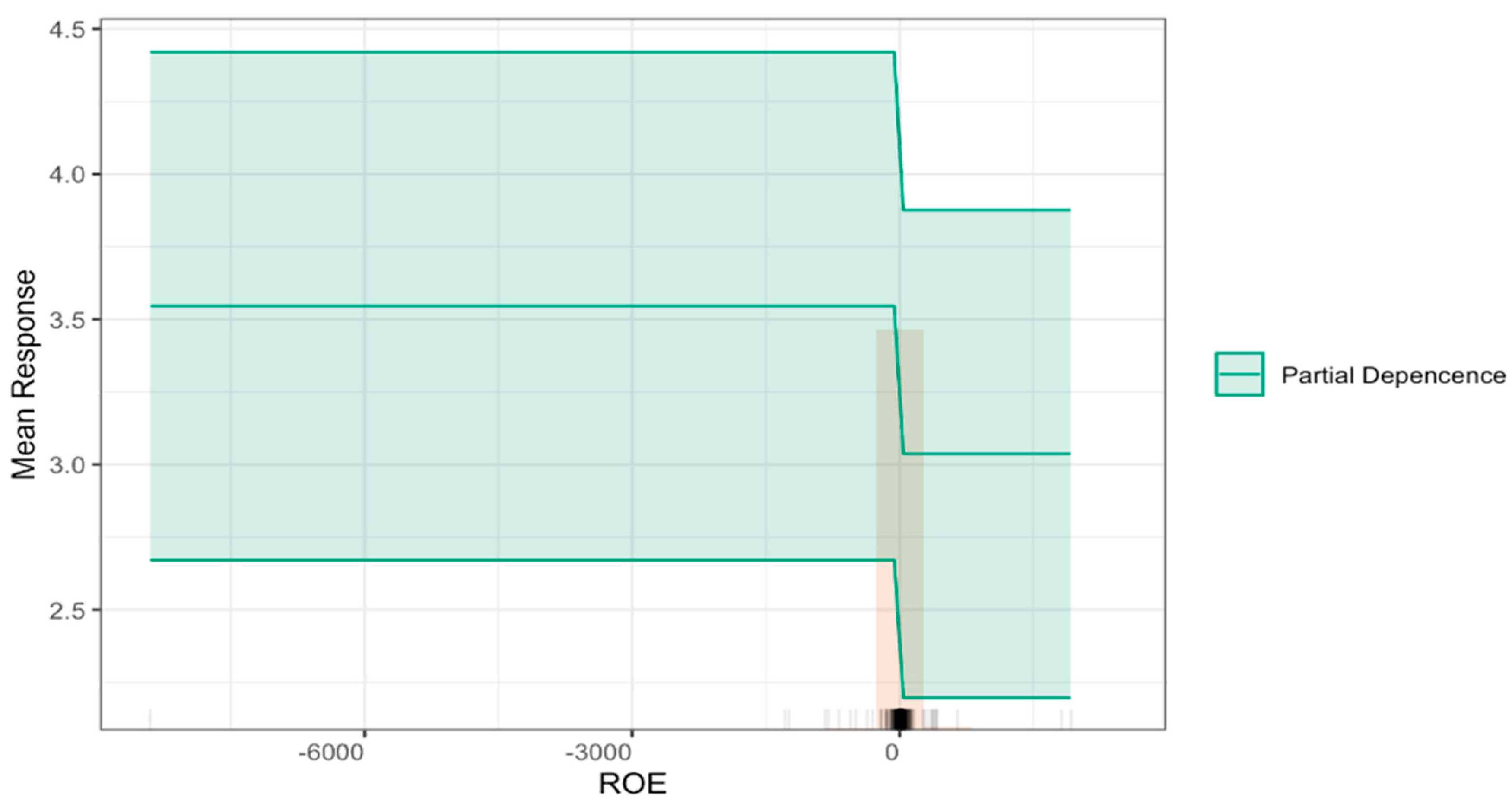
Synergy of Financial and Non-Financial Factors: liquidity (STRUC5), financial profitability (ROE), and labor costs (PREM) remain robust predictors of failure, consistent with prior studies. However, TRUCAM’s prominence highlights the necessity of integrating sustainability metrics into financial risk assessments to enhance predictive performance metrics.
3.
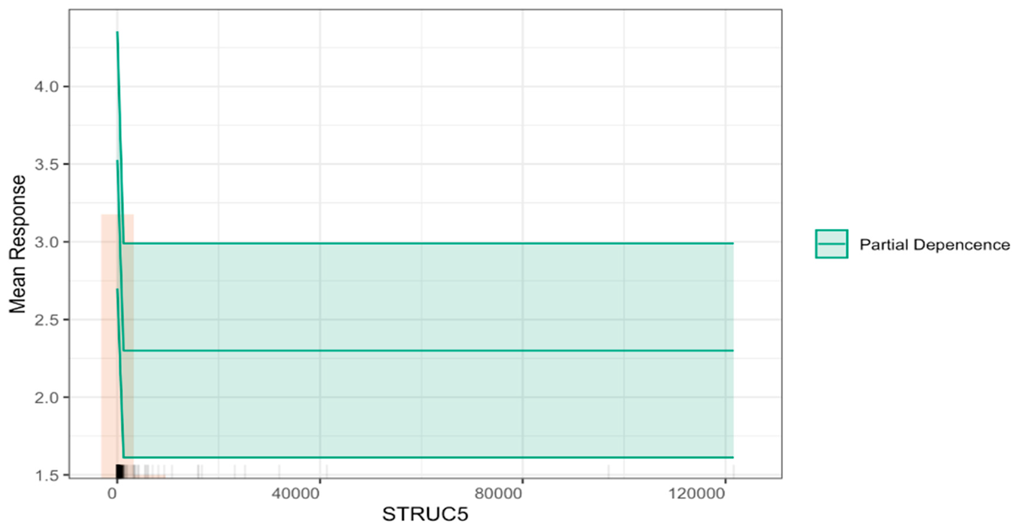
Algorithmic Efficacy and Transparency: the XGBoost algorithm proved highly effective in handling multicollinearity and nonlinear relationships. Techniques such as variable importance analysis, partial dependence plots, and break-down plots mitigated the “black box” concern, offering actionable insights into how individual variables influence specific predictions [27,41].
Our work provides a valuable and novel contribution to the existing literature, highlighting the need to integrate sustainability factors into business failure prediction models. Firms should prioritize environmental risk mitigation as a strategic imperative, recognizing its dual social and economic benefits. Policymakers are requested to incentivize sustainable practices through regulatory frameworks and fiscal measures, aligning corporate strategies with global sustainability agendas like the SDGs.
While focused on Spanish cooperatives, future studies should validate these findings across industries, geographies, and capitalist enterprises. Longitudinal analyses could capture dynamic interactions between environmental risks and failure likelihood, particularly among growing regulations.
By bridging financial and sustainability analytics, this research advances a holistic approach to business management, emphasizing that environmental risk is not merely ethical but essential for long-term corporate resilience.

Author Contributions

Conceptualization, M.R.M., P.C.I. and J.M.V.; Methodology, M.R.M., P.C.I. and J.M.V.; Software, M.R.M., P.C.I. and J.M.V.; Validation, M.R.M., P.C.I. and J.M.V.; Formal analysis, M.R.M., P.C.I. and J.M.V.; Investigation, M.R.M., P.C.I. and J.M.V.; Resources, M.R.M., P.C.I. and J.M.V.; Data curation, M.R.M., P.C.I. and J.M.V.; Writing—original draft, M.R.M., P.C.I. and J.M.V.; Writing—review & editing, M.R.M., P.C.I. and J.M.V.; Visualization, M.R.M., P.C.I. and J.M.V.; Supervision, M.R.M., P.C.I. and J.M.V.; Project administration, M.R.M., P.C.I. and J.M.V.; Funding acquisition, M.R.M., P.C.I. and J.M.V. All authors have read and agreed to the published version of the manuscript.

Funding

This research was funded by MCIU/AEI/10.13039/501100011033/FEDER/UE (Project PID2023-153128NB-I00.

Institutional Review Board Statement

Not applicable.

Informed Consent Statement

Not applicable.

Data Availability Statement

The data presented in this study are available on request from the corresponding author.

Conflicts of Interest

The authors declare no conflict of interest.

References

  1. Altman, E. Financial ratios, discriminant analysis and the prediction of corporate bankruptcy. J. Financ. 1968, 23, 589–609. [Google Scholar] [CrossRef]
  2. Zavgren, C.V. Assessing the vulnerability to failure of American industrial firms: A logistic analysis. J. Bus. Financ. Account. 1985, 12, 19–45. [Google Scholar] [CrossRef]
  3. Ohlson, J.A. Financial Ratios and the Probabilistic Prediction of Bankruptcy. J. Account. Res. 1980, 18, 109–131. [Google Scholar] [CrossRef]
  4. Alfaro, E.; Gámez, M.; García, N. A boosting approach for corporate failure prediction. Appl. Intell. 2007, 27, 29–37. [Google Scholar] [CrossRef]
  5. Delgado, M. Discurso de apertura de la Jornada “El papel de los inversores en el modelo de transición energética”. Banco De España 2019, 1–9. Available online: https://repositorio.bde.es/handle/123456789/21730. (accessed on 1 April 2024).
  6. United Nations. Transforming Our World: The 2030 Agenda for Sustainable Development (A/RES/70/1); UN General Assembly: New York, NY, USA, 2015; Available online: https://sdgs.un.org/2030agenda (accessed on 1 March 2024).
  7. Directive (EU) 2022/2464 of the European Parliament and the Council (CSRD). 2022. Available online: https://eur-lex.europa.eu/eli/dir/2022/2464/oj (accessed on 1 March 2024).
  8. United Nations Department of Economic and Social Affairs. Global Sustainable Development Report 2023; Times of Crisis, Times of Change—Science for Accelerating Transformations to Sustainable Development; United Nations Publications: New York, NY, USA, 2023. [Google Scholar] [CrossRef]
  9. Castilla-Polo, F.; García-Martínez, G.; Guerrero-Baena, M.D.; Polo-Garrido, F. The cooperative ESG disclosure index: An empirical approach. Springer Environ. Dev. Sustain. 2024, 1–26. [Google Scholar] [CrossRef]
  10. Yakar-Pritchard, G.; Tunca-Çalıyurt, K. Sustainability Reporting in Cooperatives. Risks 2021, 9, 117. [Google Scholar] [CrossRef]
  11. Duguid, F.; Rixon, D. The development of cooperative-designed indicators for the SDGs. In Handbook of Research on Cooperatives and Mutuals; Elliott, M., Boland, M., Eds.; Edward Elgar Publishing: Cheltenham, UK, 2023; pp. 333–353. [Google Scholar] [CrossRef]
  12. Abdul Aris, N.; Marzuki, M.; Othman, M.; Abdul Rahman, R.S.; Hj Ismail, N. Designing indicators for cooperative sustainability: The Malaysian perspective. Soc. Responsib. J. 2018, 14, 226–248. [Google Scholar] [CrossRef]
  13. Beaver, W.H. Financial ratios as predictors of failure. J. Account. Res. 1966, 4, 71–111. [Google Scholar] [CrossRef]
  14. Freeman, R.E. The Politics of Stakeholder Theory: Some Future Directions. Bus. Ethics Q. 1994, 4, 409–421. [Google Scholar] [CrossRef]
  15. Elkington, J. The Triple Bottom Line. Environ. Manag. Read. Cases 1997, 2, 49–66. [Google Scholar]
  16. Ben Jabeur, S.; Stef, N.; Carmona, P. Bankruptcy Prediction using the XGBoost Algorithm and Variable Importance Feature Engineering. Comput. Econ. 2023, 61, 715–741. [Google Scholar] [CrossRef]
  17. Zmijewski, M.E. Methodological issues related to the estimation of financial distress prediction models. J. Account. Rev. 1984, 22, 59–82. [Google Scholar] [CrossRef]
  18. Frydman, H.; Altman, E.I.; Kao, D.L. Introducing recursive partitioning for financial classification: The case of financial distress. J. Financ. 1985, 40, 269–291. [Google Scholar] [CrossRef]
  19. Wilson, G.I.; Sharda, R. Bankruptcy prediction using neural network. Decis. Support Syst. 1994, 11, 545–557. [Google Scholar] [CrossRef]
  20. West, D.; Dellana, S.; Qian, J. Neural network ensemble strategies for financial decision applications. Comput. Oper. Res. 2005, 32, 2543–2559. [Google Scholar] [CrossRef]
  21. Verikas, A.; Kalsyte, Z.; Bacauskiene, M.; Gelzinis, A. Hybrid and ensemble-based soft computing techniques in bankruptcy prediction: A survey. Soft Comput. 2010, 14, 995–1010. [Google Scholar] [CrossRef]
  22. Sun, J.; Li, H.; Huang, Q.H.; He, K.Y. Predicting financial distress and corporate failure: A review from the state-of-the-art definitions, modeling, sampling, and featuring approaches. Knowl.-Based Syst. 2014, 57, 41–56. [Google Scholar] [CrossRef]
  23. Kim, M.J.; Kang, D.K. Ensemble with neural networks for bankruptcy prediction. Expert Syst. Appl. 2010, 37, 3373–3379. [Google Scholar] [CrossRef]
  24. Kim, S.Y.; Upneja, A. Predicting restaurant financial distress using decision tree and adaboosted decision tree models. Econ. Model. 2014, 35, 354–362. [Google Scholar] [CrossRef]
  25. Wang, G.; Ma, J.; Yang, S. An improved boosting based on feature selection for corporate bankruptcy prediction. Expert Syst. Appl. 2014, 41, 2353–2361. [Google Scholar] [CrossRef]
  26. Jones, S.; Johnstone, D.; Wilson, R. An empirical evaluation of the performance of binary classifiers in the prediction of credit ratings changes. J. Bank. Financ. 2015, 56, 72–85. [Google Scholar] [CrossRef]
  27. Zieba, M.; Tomczak, S.K.; Tomczak, J.M. Ensemble Boosted Trees with Synthetic Features Generation in Application to Bankruptcy Prediction. Expert Syst. Appl. 2016, 58, 93–101. [Google Scholar] [CrossRef]
  28. Simti, S.; Soui, M.; Ghedira, K. Tri-XGBoost model improved by BLSmote-ENN: An interpretable semi-supervised approach for addressing bankruptcy prediction. Knowl. Inf. Syst. 2024, 66, 3883–3920. [Google Scholar] [CrossRef]
  29. Díaz, Z.; Fernández, J.; Segovia, M.J. Sistemas de inducción de reglas y árboles de decisión aplicados a la predicción de insolvencias en empresas aseguradoras. In Documentos de Trabajo de la Facultad de Ciencias Económicas y Empresariales; Universidad Complutense de Madrid: Madrid, Spain, 2004; Volume 9. [Google Scholar]
  30. Alfaro, E.; Gámez, M.; García, N. Linear discriminant analysis versus adaboost forfailure forecasting. Rev. Española Financ. Contab. 2008, 37, 13–32. [Google Scholar]
  31. Alfaro, E.; García, N.; Gámez, M.; Elizondo, D. Bankruptcy forecasting: An empirical comparison of adaboost and neural networks. Decis. Support Syst. 2008, 45, 110–122. [Google Scholar] [CrossRef]
  32. Momparler, A.; Carmona, P.; Climent, F.J. La predicción del fracaso bancario con la metodología Boosting Classification Tree. Rev. Española Financ. Y Contab. 2016, 45, 63–91. [Google Scholar] [CrossRef]
  33. Climent, F.; Momparler, A.; Carmona, P. Anticipating bank distress in the Euro-zone: An extreme gradient boosting approach. J. Bus. Res. 2019, 101, 885–896. [Google Scholar] [CrossRef]
  34. Carmona, P.; Climent, F.; Momparler, A. Predicting bank failure in the U.S. Banking sector: An extreme gradient boosting approach. Int. Rev. Econ. Financ. 2019, 61, 304–322. [Google Scholar] [CrossRef]
  35. Pozuelo, J.; Romero, M.; Carmona, P. Utility of fuzzy set Qualitative Comparative Analysis (fsQCA) methodology to identify causal relations conducting to cooperative failure. CIRIEC-España Rev. Econ. Pública Soc. Y Coop. 2023, 107, 197–225. [Google Scholar] [CrossRef]
  36. Romero, M.; Carmona, P.; Pozuelo, J. La predicción del fracaso empresarial de las cooperativas españolas. Aplicación del Algoritmo Extreme Gradient Boosting. CIRIEC-España Rev. Econ. Pública Soc. Y Coop. 2021, 101, 255–288. [Google Scholar] [CrossRef]
  37. Roffé, M.A.; González, F.A.I. El impacto de las prácticas sostenibles en el desempeño financiero de las empresas: Una revisión de la literatura. Rev. Científica Visión E Futuro 2024, 28, 195–220. [Google Scholar] [CrossRef]
  38. Confederación Española de Organizaciones Empresariales-CEOE. Catálogo 2024 de Buenas Prácticas Ambientales de las Empresas Españolas—El Esfuerzo Empresarial en la Transición Ecológica y la Descarbonización. 2025. Available online: https://www.ceoe.es/es/publicaciones/sostenibilidad/catalogo-2024-de-buenas-practicas-ambientales-de-las-empresas. (accessed on 1 March 2025).
  39. Mozas-Moral, A.; Fernández-Uclés, D.; Medina-Viruel, M.J.; Bernal-Jurado, E. The role of SDGs as enhancers of the performance of Spanish wine cooperatives. Technol. Forecast. Soc. Change 2021, 173, 121176. [Google Scholar] [CrossRef]
  40. Chen, T.; Guestrin, C. XGBoost: A scalable tree boosting system. In Proceedings of the 22nd ACM SIGKDD International Conference on Knowledge Discovery and Data Mining, San Francisco, CA, USA, 13–17 August 2016; pp. 785–794. [Google Scholar] [CrossRef]
  41. Carmona, P.; Dwekat, A.; Mardawi, Z. No more black boxes! Explaining the predictions of a machine learning XGBoost classifier algorithm in business failure. Res. Int. Bus. Financ. 2022, 61, 101649. [Google Scholar] [CrossRef]
  42. Tascón, M.T.; Castaño, F.J. Variables y Modelos para la Identificación y Predicción del Fracaso Empresarial: Revisión de La Investigación Empírica Reciente. Rev. Contab. 2012, 15, 7–58. [Google Scholar] [CrossRef]
  43. Jánica, F.; Fernández, L.H.; Escobar, A.; Pacheco, G.J.V. Factores que explican, median y moderan el fracaso empresarial: Revisión de publicaciones indexadas en Scopus (2015–2022). Rev. Cienc. Soc. 2023, 29, 73–95. [Google Scholar] [CrossRef]
  44. Romero, M.; Pozuelo, J.; Carmona, P. Ethical transparency in business failure prediction: Uncovering the black box of XGBoost algorithm. Span. J. Financ. Account./Rev. Española Financ. Y Contab. 2024, 54, 135–165. [Google Scholar] [CrossRef]
  45. SABI. Database. 2024. Available online: https://login.bvdinfo.com/R1/SabiNeo (accessed on 1 April 2024).
  46. ORBIS. Bureau Van Dijk Database. A Moody’s Analysis Firm. 2024. Available online: https://orbis.bvdinfo.com/version-20250325-3-0/Orbis/1/Companies/Search (accessed on 1 April 2024).
  47. Thomas, S.; Reppetto, R.; Dias, D. Integrated Environmental and Financial Performance Metrics for Investment Analysis and Portfolio Management. Corporate Governance: Int. Rev. 2017, 15, 421–426. [Google Scholar] [CrossRef]
  48. Meric, I.; Watson, C.D.; Meric, G. Company green score and stock price. Int. Res. J. Financ. Econ. 2012, 82, 15–23. [Google Scholar]
  49. Bolton, P.; Reichelstein, S.J.; Kacperczyk, M.T.; Leuz, C.; Ormazabal, G.; Schoenmaker, D. Mandatory Corporate Carbon Disclosures and the Path to Net Zero. Manag. Bus. Rev. 2021, 1, 21–28. [Google Scholar] [CrossRef]
  50. Bellovary, J.L.; Giacomino, D.E.; Akers, M.D. A review of bankruptcy prediction studies: 1930 to present. J. Financ. Educ. 2007, 33, 1–42. Available online: https://www.jstor.org/stable/41948574 (accessed on 5 May 2024).
  51. Friedman, J.H. Greedy function approximation: A gradient boosting machine. Ann. Stat. 2001, 29, 1189–1232. Available online: https://www.jstor.org/stable/2699986 (accessed on 5 May 2024). [CrossRef]
  52. Probst, P.; Wright, M.N.; Boulesteix, A.-L. Hyperparameters and tuning strategies for random forest. Wiley Interdiscip. Rev. Data Min. Knowl. Discov. 2019, 9, e1301. [Google Scholar] [CrossRef]
  53. Cabrera-Malik, S. Is XGBoost immune to multicollinearity? Medium. 2024. Available online: https://medium.com/@sebastian.cabrera-malik/is-xgboost-inmune-to-multicolinearity-4dd9978605b7 (accessed on 5 May 2024).
  54. James, G.; Witten, D.; Hastie, T.; Tibshirani, R. An Introduction to Statistical Learning. Springer: New York, NY, USA, 2017. [Google Scholar]
  55. Friedman, J.; Hastie, T.; Tibshirani, R. Additive logistic regression: A statistical view of boosting (with discussion and a rejoinder by the authors). Ann. Stat. 2000, 28, 337–407. [Google Scholar] [CrossRef]
  56. Hastie, T.; Tibshirani, R.; Friedman, J. The Elements of Statistical Learning; Springer: New York, NY, USA, 2009. [Google Scholar]
  57. XGBoost Parameters. Available online: https://xgboost.readthedocs.io/en/stable/parameter.html (accessed on 2 November 2024).
  58. R Core Team. R: A Language and Environment for Statistical Computing; R Foundation for Statistical Computing: Vienna, Austria, 2024; Available online: http://www.R-project.org/ (accessed on 2 November 2024).
  59. Fryda, T.; LeDell, E.; Gill, N.; Aiello, S.; Fu, A.; Candel, A.; Click, C.; Kraljevic, T.; Nykodym, T.; Aboyoun, P.; et al. h2o: R Interface for the ‘H2O’ Scalable Machine Learning Platform. R Package Version 3.44.0.3. 2024. Available online: https://CRAN.R-project.org/package=h2o (accessed on 2 October 2024).
  60. Molnar, C. Interpretable Machine Learning. 2023. Available online: https://christophm.github.io/interpretable-ml-book/ (accessed on 2 May 2024).
  61. Hall, P.; Gill, N. An Introduction to Machine Learning Interpretability, 2nd ed.; O’Reilly Media, Inc.: Sebastopol, CA, USA, 2019. [Google Scholar]
  62. Biecek, P.; Burzykowski, T. Explanatory Model Analysis. Pbiecek.github.io. 2021. Available online: https://pbiecek.github.io/ema/preface.html (accessed on 5 May 2024).
  63. Heaton, J.; Goodfellow, I.; Bengio, Y.; Courville, A. Deep learning. Genet. Program. Evolvable Mach. 2018, 19, 305–307. [Google Scholar] [CrossRef]
  64. LeCun, Y.; Bengio, Y.; Hinton, G. Deep learning. Nature 2015, 521, 436–444. [Google Scholar] [CrossRef]
  65. Candel, A.; Ledell, E. Deep Learning with H2O. 2018. Available online: https://h2o-release.s3.amazonaws.com/h2o/rel-wheeler/4/docs-website/h2o-docs/booklets/DeepLearningBooklet.pdf (accessed on 5 June 2024).
  66. Romero, M.; Carmona, P.; Pozuelo, J. Utilidad del Deep Learning en la predicción del fracaso empresarial en el ámbito europeo. Rev. Métodos Cuantitativos Para Econ. Empresa 2021, 32, 392–414. [Google Scholar] [CrossRef]
  67. Barboza, F.; Kimura, H.; Altman, E. Machine learning models and bankruptcy prediction. Expert Syst. Appl. 2017, 83, 405–417. [Google Scholar] [CrossRef]
  68. Mullainathan, S.; Spiess, J. Machine learning: An applied econometric approach. J. Econ. Perspect. 2017, 31, 87–106. [Google Scholar] [CrossRef]
  69. Natekin, A.; Knoll, A. Gradient boosting machines, a tutorial. Front. Neurorobotics 2013, 7, 21. [Google Scholar] [CrossRef]
Figure 1. Correlogram of the correlation matrix for all variables.
Sustainability 17 04948 g001
Figure 2. Correlations (and 95% confidence intervals) between all independent variables and the propensity to fail (Failure).
Sustainability 17 04948 g002
Figure 3. Identification of the ten independent variables most strongly correlated with the propensity to fail (Failure).
Sustainability 17 04948 g003
Figure 4. Learning Curve of the XGBoost Model.
Sustainability 17 04948 g004
Figure 5. Distribution of Residuals in the Validation Sample.
Sustainability 17 04948 g005
Figure 6. Importance of Variables According to the XGBoost Model. Bar Plot. The red box in the figure highlights the four most relevant features.
Sustainability 17 04948 g006
Figure 7. Variable Importance according to the XGBoost Model. Line Chart. The red box in the figure highlights the four most relevant features.
Sustainability 17 04948 g007
Figure 8. Partial Dependence Plot of the PREM Variable.
Sustainability 17 04948 g008
Figure 9. Partial Dependence Plot of the STRUC5 Variable.
Sustainability 17 04948 g009
Figure 10. Partial Dependence Plot of the ROE Variable.
Sustainability 17 04948 g010
Figure 11. Partial Dependence Plot of the TRUCAM Variable.
Sustainability 17 04948 g011
Figure 12. Break Down Plot for an Individual Observation with High Propensity to Fail according to the XGBoost Model.
Sustainability 17 04948 g012
Figure 13. Break Down Plot for an Individual Observation with Low Propensity to Fail according to the XGBoost Model.
Sustainability 17 04948 g013
Figure 14. Neuron from a hidden layer. Source: Candell and Ledell [65].
Sustainability 17 04948 g014
Figure 15. Multi-layer feedforward neural networks. Source: Candell and Ledell [65].
Sustainability 17 04948 g015
Figure 16. Reverse cumulative distribution of residuals on cross-validation data.
Sustainability 17 04948 g016
Table 1. Scale of the VADIS Financial Strength Indicator on the Bankruptcy Propensity.
Vadis P2BB Financial Strength Indicator Scale
According to Propensity to Bankruptcy:
ValueThe Company’s Risk of Bankruptcy in the Next 18 Months Is:
9More than 10 times the national average
8Between 5 and 10 times the national average
7Between 3 and 5 times the national average
6Between 2 and 3 times the national average
5Between 1 and 2 times the national average
4Between 1/2 and 1 of the national average
3Between 1/5 and 1/2 of the national average
2Between 1/10 and 1/5 of the national average
1Less than 1/10 of the national average
Source: own elaboration based on SABI database [45] and ORBIS [46].
Table 2. Explanatory variables.
KeyVariables
Structural Ratios
STRUC1Solvency ratio (%) = (Equity/Total Assets) × 100
STRUC2Equity to Fixed Assets Ratio (%) = (Equity/Non-Current Assets) × 100
STRUC3Current ratio (%) = (Current Assets/Current Liabilities) × 100
STRUC4Acid test ratio (%) = [(Current Assets − Inventories)/Current Liabilities] × 100
STRUC5Cash Ratio (%) = (Cash + Cash Equivalents)/Current Liabilities) × 100
DEBT1Debt to Capital Ratio (%) = [Non-commercial Liability/(Equity + Total Liabilities)] × 100
DEBT2Liabilities to Equity Ratio = (Total Liabilities/Equity) × 100
DEBT3Gearing (%) = (Non-Current Liabilities + Loans/Equity) × 100
LEVERLeverage Ratio = Return on Assets (ROE)/Return on Equity (ROA)
INTERDebt Service Coverage Ratio (%) = (Non-Commercial Liability/Cash Flow) × 100
CASH1Cash Flow Margin (%) = (Cash Flow/Net Turnover) × 100
CASH2Cash Return on Assets (%) = (Cash Flow/Total Assets) × 100
BREAKBreak-even Ratio = Net turnover/(Net Turnover − EBIT) × 100
Operating Ratios
ROTASAsset Turnover Ratio = Net Turnover/Total Assets
AVCOLAverage Collection Period (days) = (Debtors/Net Turnover) × 360
AVPAYAverage Payment Period (days) = [Suppliers/(Procurement + External Services)] × 360
Profitability Ratios
ROAReturn on Assets (%) = (EBIT/Total Assets) × 100
PROPEOperating Profitability (%) = (EBITDA/Total Assets) × 100
ROEReturn on Equity (%) = (Net Income/Equity) × 100
PREMCost of employee/Oper. Rev = (Personnel Expenses/Operating Revenue) × 100
Environmental Variable
TRUCAM: Trucost Environmental Scores
Source: Own elaboration based on SABI database (2024) [45].
Table 3. Main descriptive statistics of the variables most strongly correlated with the Failure variable.
MeanSDMedianMinMaxSkewSE
STRUC142.9940.7545.33−392.09100.00−3.291.31
DE
BT2
57.0140.7554.670.00492.093.291.31
DEBT125.7430.6217.340.00358.773.230.98
AVPAY60.16247.1323.17−958.455936.3416.307.93
STRUC5626.035480.3149.910.00121,634.2917.54175.87
STRUC3895.586636.64157.181.33160,265.2418.71212.98
STRUC4827.006603.00123.000.0016,065.001898.00212.00
PREM26.8027.7817.690.00225.541.880.89
TRUCAM12.4821.603.160.2673.182.070.69
STRUC21130.4016,570.81104−126,016393,41217.66531.78
Failure3.231.443.001.009.001.060.05
Notes. N = 971.
Table 4. Summary of Model Performance Results.
XGBoost
RMSE (Training sample)0.768
RMSE (Cross-validation samples)1.209
RMSE (Validation sample)1.314
Table 5. Performance metrics of the three fitted regression models on validation data.
ModelMSERMSEMAEMean Residual Deviance
XGBoost1.7271.3141.0031.727
OLS Regression2.5981.6121.2262.598
Deep Learning2.5051.5831.4002.505
Disclaimer/Publisher’s Note: The statements, opinions and data contained in all publications are solely those of the individual author(s) and contributor(s) and not of MDPI and/or the editor(s). MDPI and/or the editor(s) disclaim responsibility for any injury to people or property resulting from any ideas, methods, instructions or products referred to in the content.

