Abstract
This paper explores the impact of trade openness and exchange rate volatility on South Africa’s industrial growth from 1980 to 2024 through a hybrid econometric framework combining Autoregressive Distributed Lag (ARDL) and Structural Vector Autoregression (SVAR) models. It captures both long-term relationships and short-term economic patterns; the analysis reveals that gross domestic product (GDP) is the most significant and consistent driver of industrial value added (IVAD), while trade openness and currency volatility exert limited standalone effects. Structural shocks, notably the 2008 global financial crisis and the COVID-19 pandemic, had significant negative short-term impacts on industrial performance, highlighting systemic vulnerabilities. Robustness tests, including rolling window ARDL and first-difference GDP estimation, confirm the persistence of these relationships. Impulse response functions and forecast error variance decomposition underscore the transient and moderate influence of external shocks compared with the dominant role of internal macroeconomic fundamentals. These findings indicate that liberalisation and exchange rate flexibility must be embedded within a broader developmental strategy underpinned by institutional strength, resilience building, and sustainability principles. This study provides fresh insights supporting policy frameworks that prioritise domestic industrial capacity, macroeconomic stability, and alignment with Sustainable Development Goal 9—inclusive and sustainable industrialisation.
1. Introduction
Industrial development remains a fundamental pillar of long-term economic transformation, especially within emerging economies such as South Africa’s. Over the past four decades, South Africa has undergone profound structural adjustments, transitioning from a protected, inward-looking economy to one increasingly open to global markets. While trade liberalisation has facilitated integration into global value chains and enhanced competitiveness, it has also heightened exposure to external shocks, particularly exchange rate volatility and global financial disruptions. These evolving dynamics raise pressing questions regarding the sustainability and resilience of South Africa’s industrial expansion in an increasingly volatile global economic environment [1].
Trade openness, commonly measured by the trade-to-GDP ratio, is frequently cited as a key driver of industrial development expanding market access, encouraging competition, fostering efficiency, and enabling technological diffusion. However, these gains are not automatic. They are deeply contingent upon a country’s institutional quality, industrial absorptive capacity, and coherence in complementary policy frameworks [2]. Recent empirical studies affirm that while trade liberalisation may catalyse growth, its effectiveness is considerably amplified in environments underpinned by robust institutions and cohesive industrial policies [3].
Concurrently, exchange rate instability has emerged as a formidable constraint on industrial growth, particularly in economies dependent on imported inputs and global export competitiveness. Fluctuating currency values complicate investment planning, inflate production costs, and undermine long-term industrial viability. Although depreciation may temporarily boost export revenues, persistent volatility undermines firm-level confidence and macroeconomic predictability, both of which are essential for industrial deepening in open economies like South Africa [4].
While a substantial body of literature has separately examined trade openness and exchange rate volatility, their interactive effects on industrial performance remain insufficiently explored. Most studies have centred on aggregate economic indicators rather than sector-specific outcomes such as industrial value added. Moreover, few have accounted for the role of major structural disruptions such as global crises in shaping the interplay between openness and volatility. This gap is particularly striking given the emphasis on inclusive and sustainable industrialisation within frameworks like the United Nations Sustainable Development Goals (e.g., SDG 9) [5].
This study aims to bridge these gaps by examining the joint influence of trade openness and exchange rate volatility on South Africa’s industrial growth between 1980 and 2024. Using a hybrid modelling strategy that combines Autoregressive Distributed Lag (ARDL) and Structural Vector Autoregression (SVAR) techniques, this study captures both long-run equilibrium dynamics and short-run responses to macroeconomic shocks. Structural breaks such as the post-apartheid liberalisation, the 2008 global financial crisis, and the COVID-19 pandemic are explicitly incorporated to contextualise and strengthen inference [6].
This study makes three core contributions. First, by integrating ARDL and SVAR models, it provides a methodologically robust framework for examining both equilibrium relationships and dynamic interactions among industrial growth determinants. Second, it anchors the findings within the broader sustainable development agenda, linking empirical results to objectives such as resilience building, inclusive industrialisation, and macroeconomic sustainability. Third, it underscores the foundational role of macroeconomic stability, demonstrating that industrial policies cannot yield sustained outcomes in the absence of currency stability and institutional strength. Collectively, these contributions offer new insights for policy design, particularly in middle-income economies grappling with liberalisation trade-offs [7].
The remainder of the paper is structured as follows: Section 2 reviews the literature on trade openness, exchange rate volatility, and industrial growth, identifying key empirical patterns and methodological limitations. Section 3 outlines the data sources, variable transformations, and econometric strategy. Section 4 presents the empirical results and interprets the long-run and short-run dynamics using ARDL and SVAR models. Section 5 concludes with policy implications, study limitations, and avenues for future research.
2. Literature Review
2.1. Trade Openness and Industrial Growth
Trade openness is often regarded as a key driver of industrial growth, primarily through improved market access, technology spillovers, and competitive efficiencies. Classical and endogenous growth theories both highlight the role of trade in enhancing productivity via specialisation and innovation diffusion. More recently, evidence has emphasised that openness also facilitates access to diverse intermediate inputs and advanced production technologies, thereby stimulating industrial output in developing economies [8].
Empirical evidence from South Africa presents a mixed picture. Some studies associate trade openness with improved industrial performance, particularly when accompanied by institutional reforms and export incentives. For instance, findings by [9,10] suggest that trade liberalisation contributed to upgrading in specific sectors. These results align with broader developing country experiences, where openness spurs industrialisation under conducive policy environments [11].
However, openness alone does not guarantee industrial success. Without targeted industrial policies and strong institutional frameworks, exposure to international competition may trigger premature deindustrialisation. Refs. [12,13] argue that meaningful gains from liberalisation materialise only after surpassing thresholds in infrastructure, human capital, and governance. As such, the literature increasingly points to the conditional benefits of trade openness emphasising the need to reinforce domestic industrial capabilities to fully leverage external integration.
Contemporary literature also stresses the importance of aligning trade policy with environmental and social objectives. Refs. [14,15] observe that integrating environmental safeguards and labour standards into trade regimes enhances industrial resilience and inclusiveness. This reflects the broader sustainable development imperative where industrial policy must simultaneously advance economic, social, and environmental goals.
South Africa’s industrial experience further illustrates these challenges. Despite liberalisation, the manufacturing sector remains concentrated, import dependent, and structurally constrained. As noted in [16], openness has not translated into broad-based diversification. This underscores the need for targeted policies that foster local capacity, stimulate technological upgrading, and promote green industrial transformation [17].
2.2. Exchange Rate Volatility and Industrial Growth
Exchange rate volatility also poses a formidable obstacle to sustained industrial growth, particularly in economies reliant on imported inputs or foreign markets. Volatile exchange rates complicate production and investment planning, distort cost structures, and reduce long-term competitiveness [18]. While occasional depreciation may improve export margins, persistent instability undermines investor confidence and macroeconomic predictability [18].
South African data support these concerns. Studies [19,20] demonstrate a strong negative relationship between rand volatility and manufacturing output. This mirrors broader emerging market evidence, where currency swings constrain industrial performance through higher costs and reduced trade competitiveness. The cumulative effect is often lower industrial investment and output [21].
Notably, the effects of exchange rate instability are not uniform. Economies with deeper financial markets and innovative firms are better positioned to absorb currency shocks. Instruments such as hedging contracts and diversification strategies can mitigate volatility. However, in South Africa, such mechanisms have proven insufficient, with [22] highlighting persistent vulnerabilities despite financial market development.
In South Africa’s context, however, even a relatively advanced financial system has not fully shielded the industrial sector from currency instability. Ref. [22] notes that persistent rand volatility continues to undermine manufacturing performance despite the presence of financial instruments and policies aimed at stabilisation. This indicates limits to what financial development can achieve in the face of frequent external shocks. Refs. [21,23] similarly show that exchange-rate fluctuations amplify industrial fragility in emerging economies when macroeconomic buffers, such as prudent monetary policy and fiscal space, are weak. South Africa’s experience aligns with this: episodes of high volatility have often coincided with broader macroeconomic imbalances, making industries more susceptible to the compounded effects of currency swings and domestic instability. Thus, achieving industrial resilience in an open economy like South Africa requires striving for exchange rate stability through sound macroeconomic management and deeper structural transformation [24,25]. The literature indicates that building a more technology-intensive and diversified industrial base is crucial so that the economy is less reliant on volatile commodity-linked revenues and can better withstand external financial shocks [7,21,26]. In summary, stable macroeconomic conditions and proactive risk management are foundational to insulating the industrial sector from exchange-rate volatility, enabling more consistent long-term growth.
2.3. Combined Effects of Trade Openness and Exchange Rate Volatility
While extensive research has examined trade openness and exchange rate volatility independently, studies exploring their combined impact on industrial growth remain sparse. Theoretically, high trade openness can amplify the transmission of currency shocks to domestic industries, exacerbating output volatility [27,28,29]. This is particularly true in sectors with low local value addition or high import intensity.
Recent empirical work supports this interaction hypothesis. For example, Refs. [30,31] show that trade-exposed industries suffer disproportionately during periods of exchange rate instability. In these contexts, volatility can erode the gains from openness and reverse industrial progress.
Earlier research often failed to capture these joint effects due to methodological limitations. Traditional ARDL or VAR models may overlook structural breaks and non-linear dynamics inherent in periods of crisis. In response, recent scholarship advocates hybrid models that combine long-run analysis with structural shock identification such as the ARDL–SVAR framework used in this study.
For South Africa, a strategic blend of trade liberalisation and macroeconomic stabilisation is essential to enhance industrial resilience. Participation in initiatives such as AfCFTA should be coupled with investments in local value chains, exchange rate buffers, and technological upgrading. Countries that navigate the openness–volatility nexus effectively tend to have robust institutions, fiscal discipline, and innovation-led industrial policy.
3. Materials and Methods
3.1. Data Sources and Variable Transformation
This study utilises annual time-series data spanning the period 1980 to 2024, giving a total of 45 balanced observations per variable. The choice of annual data is justified on two grounds: first, the nature of industrial growth in South Africa is influenced by slow-moving macroeconomic forces and long-term policy interventions; second, the availability and consistency of historical data over four decades is significantly stronger at an annual frequency, particularly for trade, industrial value added, and macroeconomic indicators.
The core variables selected reflect both domestic fundamentals and external economic dynamics. These include the following:
- Industrial Value Added (IVAD)—measured in constant local currency units, sourced from the World Bank World Development Indicators (WDI), and representing the dependent variable in this study.
- Trade Openness (TROP)—defined as the ratio of total trade (exports + imports) to GDP. The variable is computed using WDI-sourced export, import, and GDP data.
- Exchange Rate (EXCH)—measured as the average annual exchange rate of the South African rand to the US dollar (ZAR/USD).
- Exchange Rate Volatility—derived as the annualised standard deviation of monthly nominal exchange rate values, as follows:
σt = √((1/n) × Σ (ei − μ)2)
- σt is the volatility in year t;
- ei is the exchange rate in month i;
- μ is the average exchange rate over the year;
- n = 12 months.
This approach captures intra-annual variability and approximates the macro uncertainty that investors and producers face during production and export planning.
- Inflation (INFL)—measured as the annual percentage change in CPI (Consumer Price Index, base year 2015 = 100).
- Gross Domestic Product (GDP)—constant local currency unit GDP used to capture aggregate domestic economic activity.
- Dummy Variables—to isolate the effects of structural shocks, the following binary variables were defined:
- DUM1994 = 1 for 1994 onwards, to mark the onset of liberalisation and democratic reform (which was not significant).
- DUM2008 = 1 for the global financial crisis period (2008–2010).
- DUM2020 = 1 for the COVID-19 shock period (2020–2022).
These dummy variables are structured to avoid post-crisis persistence bias by limiting their scope to the immediate shock duration. All continuous variables are transformed using the natural logarithm to linearise exponential growth trends and interpret the estimated coefficients as elasticities. Dummy variables remain untransformed.
3.2. Research Design and Econometric Justification
This study adopts a hybrid modelling strategy, combining the Autoregressive Distributed Lag (ARDL) framework and the Structural Vector Autoregression (SVAR) approach. This dual strategy serves complementary purposes: the ARDL bounds testing technique is employed to identify long-run relationships and short-run adjustments, while the SVAR framework captures dynamic interdependencies and the transmission of structural shocks. This methodological choice ensures a comprehensive treatment of the key economic relationships, accommodating integration orders of I(0) and I(1), and providing flexibility for causality and contemporaneous impact tracing. The design recognises the possibility of feedback loops and lagged impacts, especially in the context of trade openness and exchange rate dynamics.
3.2.1. ARDL Bounds Testing Approach
The ARDL model, developed by [32] and used by [33], is suited for small sample macroeconometric analysis and is effective when regressors are of mixed integration orders, but not I(2). The long-run ARDL equation used is
The bounds testing procedure tests the null hypothesis of no cointegration among the regressors. If the F-statistic exceeds the upper-bound critical value, a long-run relationship is confirmed. Once cointegration is established, the model is re-specified in an error correction form as
where
- π captures the speed of adjustment to long-run equilibrium and is expected to be negative and significant;
- are first-differenced lagged explanatory variables.
The inclusion of GDP, despite IVAD being part of GDP, is justified to account for broader macroeconomic cycles, including consumption, investment, and government expenditure shocks. Correlation matrices and Variance Inflation Factor (VIF) analysis confirmed that no serious multicollinearity is present (all VIF < 4). Robustness tests using models that exclude GDP and replace it with ∆GDP (growth rate) show consistent sign and size of other coefficients, affirming model stability.
3.2.2. Structural Vector Autoregression (SVAR) Specification
To assess the contemporaneous and lagged structural effects of trade and exchange rate shocks on industrial output, a Structural Vector Autoregression (SVAR) model is estimated. The reduced-form VAR model takes the form
where Yt = [IVAD,TROP,EXCH], and ut is a vector of reduced-form errors.
The structural form is
where B is the contemporaneous impact matrix and εt represents orthogonal structural shocks.
The identification of the SVAR is achieved via Cholesky decomposition with the ordering
IVAD → TROP → EXCH
This ordering assumes the following:
- IVAD (industrial value added) responds only to its own contemporaneous innovations within the period.
- TROP (trade openness) can be contemporaneously affected by IVAD.
- EXCH (exchange rate volatility) can be contemporaneously affected by both IVAD and TROP.
This recursive structure is consistent with the argument that industrial performance sets the pace for trade expansion and currency market reactions, especially in an economy like South Africa where productive capacity underpins export dynamics. Impulse response functions (IRFs) are derived to trace the effect of a one-time standard deviation shock to one variable on the others over a multi-period horizon. Forecast error variance decompositions (FEVDs) identify the proportion of the forecast error variance of each variable that can be attributed to shocks in other variables.
3.3. Estimation Procedure
The empirical estimation follows this sequential procedure:
- Stationarity Testing—The Augmented Dickey–Fuller (ADF) and Phillips–Perron (PP) unit root tests are applied to each series to determine the order of integration.
- Cointegration Testing (ARDL Bounds Test)—Once the variables are confirmed to be I(0) or I(1), bounds testing is performed to confirm long-run cointegration. Critical values at 1%, 5%, and 10% significance are used for interpretation.
- ARDL and Error Correction Modelling—The optimal lag structure is chosen based on the Akaike Information Criterion (AIC), and the long-run coefficients are estimated.
If cointegration is established, the ECM is estimated to evaluate short-run dynamics and the adjustment speed.
- Robustness Checks—Three ARDL robustness checks are conducted, as follows:
- ○
- A model excluding exchange rate volatility (EXCH) to test its marginal contribution;
- ○
- A model using the rolling window ARDL model to measure the consistency of cointegration over the period studied;
- ○
- A model using GDP growth (∆GDP) instead of GDP level to control for potential endogeneity and trend bias.
- SVAR Estimation—The selected variables are transformed to a stationary form before VAR estimation. The optimal lag length is determined using AIC and the Schwarz Bayesian Criterion (SBC). The system is identified using a lower triangular Cholesky matrix. Post-estimation diagnostics include tests for serial correlation (Breusch–Godfrey), residual normality (Jarque–Bera), heteroskedasticity (ARCH), and system stability (eigenvalue analysis).
This comprehensive econometric strategy ensures rigour in long-run analysis, dynamic identification of structural shocks, and empirical robustness under various specifications. The design addresses model endogeneity, identifies macroeconomic channels of influence, and prepares a platform for policy-relevant insights in Section 5.
4. Results and Discussion
4.1. Unit Root and Stationarity Tests
Before estimating the ARDL and SVAR models, unit root tests were conducted to determine the integration order of each series. The analysis uses 45 annual observations per variable from 1980 to 2024. Both the Augmented Dickey–Fuller (ADF) and Phillips–Perron (PP) [34] tests were applied, with and without trends, to each variable. All variables except GDP and IVAD were found to be non-stationary in levels but stationary in first differences, justifying the use of ARDL bounds testing for cointegration. GDP and IVAD appear stationary in level form (at least with an intercept included), indicating that they are I(0), whereas trade openness (TROP), exchange rate (EXCH), and inflation (INFL) are I(1). The mix of I(0) and I(1) variables supports the suitability of the ARDL approach. The key unit root findings are summarised in Table 1, which underpins our ARDL and SVAR modelling strategy.

Table 1.
Unit root test results.
Given the possibility of endogeneity between GDP and industrial output, future research could consider instrumental variable approaches or apply structural equation modelling (SEM) to disentangle causal flows more explicitly. In this study, GDP is treated as a macroeconomic driver capturing broader cyclical dynamics. VIF analysis confirmed no problematic multicollinearity, and results are robust to model the exclusion of GDP. While this study adopts GDP as exogenous in the ARDL specification, bidirectional influence cannot be entirely ruled out.
4.2. Cointegration Analysis: ARDL Bounds Test
Using the ARDL bounds test with a mix of I(0) and I(1) variables and evidence of potential cointegration, we proceed with the ARDL bounds testing approach. The ARDL bounds test for cointegration was applied among IVAD, TROP, EXCH, and the control variables (GDP, INFL, plus crisis dummies). The dummy variables DUM2008 and DUM2020 are limited to the years 2008–2010 and 2020–2022, respectively, to reflect the immediate shock period and avoid long-horizon distortion. The computed F-statistic of 6.73 lies well above the 5% critical upper bound (approximately 3.79) [32], firmly rejecting the null hypothesis of no long-run relationship. In other words, the evidence indicates a stable long-run cointegration between industrial output and the covariates in the model [35]. Table 2 underscores the ARDL bounds test results.
Table 2.
ARDL bounds test results (dependent variable: IVAD).
Having established cointegration, we estimated the long-run coefficients via the ARDL (1,1,1,1,1,1) model. Table 3 reports the estimated long-run coefficients. GDP is by far the most essential determinant: its long-run coefficient is positive (~4.31) and highly significant. This result is consistent with the endogenous growth theory [36] that links sustained national income growth to industrial expansion. In practical terms, a 1% permanent increase in GDP is associated with roughly a 4.3% rise in industrial value added in the long run, holding other factors constant (Table 3). By contrast, trade openness and exchange rate instability have coefficients near zero and are statistically insignificant. This result aligns with the mixed results in [3,9,37] (which found that the tradable sector had little impact on the economy). This indicates that, over the past decades, liberalisation (higher TROP) and rand volatility alone did not translate into higher industrial output. One interpretation is that South Africa’s industry may face structural constraints or weak absorptive capacity; openness without complementary policies or institutions may have yielded little automatic gain. This result aligns with [13,37,38]. To summarise, GDP growth drives the long-run cointegration relationship almost entirely, while the expected channels via trade or exchange rates appear muted in our sample.
Table 3.
Estimated long-run coefficients.
Table 4 also includes two dummy variables capturing major shocks. The 2008 global financial crisis dummy is negative (−0.1174) and marginally significant (p ≈ 0.088), and the 2020 COVID dummy is strongly negative (−0.3382, p < 0.01). These signs are intuitive: such crises pulled down industrial output substantially. The significant negative dummies emphasise that external shocks can temporarily derail South Africa’s industrial performance.
4.3. Short-Run Dynamics and Error Correction Model (ECM)
The next step is to examine the short-run dynamics using the error correction model (ECM) associated with the ARDL. The error correction term (the lagged cointegration residual) has an estimated coefficient of about −0.5272 in the complete model (Table 4). This indicates that roughly 52.7% of any deviation from the long-run equilibrium is corrected within 1 year. In other words, the disequilibrium generated by a shock is more than half eliminated by the next period, indicating a relatively rapid adjustment to the cointegrating path.
In the short run, changes in GDP continue to exert a strong positive effect on industrial output. The coefficient on ΔGDP is about 1.1186, confirming that year-to-year growth spurts immediately boost industrial value added. This result is in alignment with the findings in [30]. By contrast, the first differences of trade openness (ΔTROP) and exchange rate (ΔEXCH) remain statistically insignificant, and this result aligns with [31]. This means that short-lived openness or currency value fluctuations did not translate into measurable industrial gains (or losses) in the short term. Inflation changes (ΔINFL) also show no significant short-run impact in alignment with [39], suggesting that moderate inflation fluctuations did not materially affect industrial growth over this period. Indirect effects, such as how exchange rate instability influences import prices, export earnings, or investment sentiment, could be incorporated into a future extended SVAR or mediation analysis framework to capture second-round effects on industrial output.
The crisis dummies, however, remain highly significant with negative coefficients (DUM2008 ≈ −0.0360, p ~ 0.01; DUM2020 ≈ −0.0490, p < 0.01). This again highlights the disruptive effect of the financial crisis and pandemic shocks: industrial output fell sharply relative to the trend during those episodes.
This study also re-estimated the ECM without the exchange rate term (see Table 5). This alternative specification yields nearly identical qualitative results: GDP remains strongly positive, the dummies remain significantly negative, and the ECM term is −0.5133. Model fit is marginally improved, but there are no substantive changes. The robustness of these results suggests that exchange rate instability per se provided little additional explanatory power for the short-run industrial dynamics, consistent with the insignificance of EXCH in the long run.
Table 5.
ECM estimates (excluding EXCH).
Table 4.
ECM estimates (including EXCH).
Table 4.
ECM estimates (including EXCH).
| Variable | Coefficient | Std. Error | t-Statistic | p-Value |
|---|---|---|---|---|
| Const | −0.0113 | 0.0032 | −3.51 | 0.0009 *** |
| ΔGDP | 1.1186 | 0.0811 | 13.79 | 0.0000 *** |
| ΔINFL | 0.0079 | 0.0060 | 1.32 | 0.1917 |
| ΔEXCH | −0.0101 | 0.0170 | −0.60 | 0.5540 |
| ΔTROP | 0.0357 | 0.0410 | 0.87 | 0.3870 |
| DUM2008 | −0.0360 | 0.0142 | −2.53 | 0.0144 ** |
| DUM2020 | −0.0490 | 0.0154 | −3.18 | 0.0025 *** |
| −0.5272 | 0.1536 | −3.43 | 0.0012 *** |
Note: ***, ** denote significance at 1%, 5% levels, respectively. Source: author’s computation.
4.4. Diagnostic Checks for the ECM Models
Standard diagnostic tests confirm that the ECM specifications are well behaved (see Table 6). Breusch–Godfrey (Ljung–Box) tests find no evidence of serial autocorrelation, and ARCH tests show no autoregressive conditional heteroskedasticity. The residuals appear normally distributed (Anderson–Darling p > 0.4). A Ramsey RESET test also fails to reject the correct functional form [40]. Recursive CUSUM and CUSUMSQ plots indicate that parameter estimates are stable over time. Altogether, these diagnostics give confidence in the validity of the ARDL/ECM results.
Table 6.
Diagnostic test results for ECM models.
4.5. Additional Robustness Checks
To further validate the stability and generalisability of the ARDL–SVAR findings, two supplementary robustness tests were undertaken beyond the previously reported alternative ECM model that excluded the exchange rate variable. These tests provide further assurance that the study’s core conclusions are not model dependent or sensitive to sample selection, variable transformations, or structural breaks.
4.5.1. Rolling Window ARDL Estimation
The first test involved estimating rolling window ARDL regressions across overlapping 25-year sub-periods to detect potential instability in the long-run relationships. As shown in Table 7, the coefficient on GDP remained strongly positive and statistically significant across all windows, with values consistently around 4.3 and p-values below 1%. This reaffirms that industrial value added (IVAD) is persistently driven by domestic economic performance. In contrast, trade openness (TROP) and exchange rate volatility (EXCH) remained insignificant throughout, confirming that their limited role in industrial growth holds over time and under changing structural conditions. The crisis dummies (DUM2008 and DUM2020) remained negative, with growing statistical significance in later windows, further confirming the destabilising effects of external shocks on industrial performance. These findings mirror those in the baseline ARDL model (Table 3) and ECM specifications (Table 4 and Table 5), demonstrating the temporal robustness of the model estimates and lending greater weight to policy recommendations that prioritise domestic capacity development over unqualified liberalisation.
Table 7.
Rolling window ARDL estimates (window = 25 years).
4.5.2. ARDL Estimation Using ΔGDP
The second robustness test re-estimated the ARDL model by replacing GDP levels with its first difference (ΔGDP), thereby capturing the influence of economic growth rate rather than output size. As reported in Table 8, the ΔGDP coefficient remained highly significant (p < 0.01), with a magnitude of approximately 1.095, implying that even temporary improvements in GDP growth exert a strong and immediate impact on industrial output. Notably, the core results remained consistent with earlier findings: trade openness and exchange rate volatility continued to exhibit statistically insignificant effects, while the crisis dummies retained their negative signs and significance. The ECM coefficient (−0.5189) also closely aligned with that from previous specifications, reinforcing the rapid speed of adjustment toward long-run equilibrium. This specification confirms that industrial performance is robustly explained by macroeconomic expansions, regardless of whether GDP is measured in levels or rates of change. These results confirm that the industrial sector in South Africa is primarily responsive to domestic economic activity, irrespective of whether it is measured in levels or growth rates, and that external openness or currency volatility lacks an autonomous impact without stronger structural enablers.
Table 8.
ARDL (1,1,1,1,1,1) with GDP growth rate.
Collectively, the results from Table 7 and Table 8 demonstrate that the core ARDL–SVAR findings are not driven by arbitrary model design or data artefacts. The robustness of GDP’s effect, coupled with the consistent insignificance of TROP and EXCH, suggests that trade liberalisation and currency exposure do not automatically yield industrial growth benefits. Instead, as supported by the broader literature [31,37,38], these external variables likely interact with domestic institutions, productive capabilities, and policy environments to generate conditional outcomes. Hence, industrial policy should remain grounded in strengthening internal economic fundamentals, which are demonstrably the most reliable predictors of long-term industrial expansion in South Africa.
4.6. SVAR Estimation: Impulse Response and Variance Decomposition
Following the validation of the ECM, the analysis proceeds to examine short-run structural dynamics through a Structural Vector Autoregression (SVAR) model. The SVAR model is estimated using the same annual sample from 1980 to 2024, with consistent variable transformation and dummy treatment across both modelling frameworks. The SVAR complements the ARDL framework by focusing on first-differenced data for industrial value added (IVAD), exchange rate changes (ΔEXCH), and trade openness changes (ΔTROP), thereby capturing the immediate interactions among these variables in response to exogenous shocks. Prior to estimation, the Johansen cointegration test was applied and confirmed the absence of long-run cointegration relationships among the differenced series, thereby justifying the use of a VAR in differences [41]. Using three standard information criteria (AIC, SBC, HQ), all three measures unanimously selected a lag length of two, striking an optimal balance between model fit and parsimony.
The SVAR model was identified using a recursive Cholesky decomposition, consistent with [42], ordering the variables as IVAD → ΔTROP → ΔEXCH. This ordering assumes that industrial value added has a contemporaneous influence on trade and exchange rate conditions, and that trade affects exchange within the same year. It reflects the premise that, in South Africa’s context, industrial dynamics lead short-run macroeconomic adjustments. Robustness checks using alternative ordering schemes yielded similar results, reinforcing the stability of the identification strategy.
4.6.1. Impulse Response Functions (IRFs)
Figure 1 shows the impulse response functions from the SVAR, which reveal how industrial output reacts to trade openness and exchange rate shocks. A one-standard-deviation positive shock to ΔTROP is associated with a modest rise in IVAD: the response turns significantly positive after about two periods and peaks around period 5 before stabilising, which aligns with findings in [31]. In contrast, a one-standard-deviation shock to ΔEXCH induces an immediate dip in IVAD, aligning with [30]. Interestingly, however, this negative impact decays quickly, and IVAD returns to baseline within three to four periods.
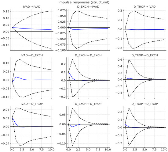
Figure 1.
Impulse response functions (IVAD to ΔEXCH and ΔTROP). Source: author’s SVAR computation. Note: the dashed lines are the 95% confidence intervals, and the solid line is the impulse response function.
4.6.2. Forecast Error Variance Decomposition (FEVD)
The FEVD results quantify the relative importance of each shock. Table 9 underscores that, after 10 periods, IVAD’s own shocks explain ~87.9% of its variance, with 8.8% attributable to exchange rate shocks and 3.3% to trade shocks. Table 10 indicates that ΔEXCH’s forecast variance is dominated (83.7%) by its own shocks, with 4.6% explained by IVAD shocks and 11.6% by trade shocks. Table 11 shows that ΔTROP’s variance is ~68.1% self-driven, with 9.9% explained by exchange rate shocks and 22.0% by IVAD shocks (the latter aligning with the idea that domestic output conditions can influence trade performance, as per [23].
Table 9.
FEVD for IVAD (% of variance explained, with 95% CI).
Table 10.
FEVD for ΔEXCH (% of variance explained, with 95% CI).
Table 11.
FEVD for ΔTROP (% of variance explained, with 95% CI).
Overall, the RDL–ECM results indicate that South Africa’s industrial growth is driven primarily by domestic economic performance (GDP), with trade openness and exchange rate instability playing a secondary role in both the long run and the short run. External crises have noticeable negative impacts, reflected in dummy variables. The SVAR analysis further highlights that while trade openness shocks can have positive but modest effects on industrial output, exchange rate instability shocks tend to have negative but short-lived effects, with industrial output proving relatively resilient after the initial impact. These findings indicate that internal economic fundamentals and stability are crucial for South Africa’s industrial growth, and that the direct benefits of openness or costs of volatility are present but moderated by other factors.
5. Conclusions, Policy Implications, and Future Research
5.1. Conclusions
This study provides robust empirical evidence on the drivers of South Africa’s industrial growth using a hybrid ARDL–SVAR model from 1980 to 2024. The results demonstrate that domestic economic performance, particularly GDP, plays a crucial role in shaping industrial value added (IVAD), with external variables such as trade openness and exchange rate volatility showing limited standalone effects. These findings underscore the critical importance of internal macroeconomic stability and productive capacity in enabling industrial development.
The analysis confirms that global crises, notably the 2008 financial crisis and the COVID-19 pandemic, had severe negative impacts on industrial growth. Trade openness, while theoretically conducive to industrial expansion, does not automatically generate growth unless paired with supportive domestic conditions. Similarly, exchange rate volatility introduces uncertainty that undermines investment and competitiveness, although its effects are relatively short-lived.
By integrating both long-run equilibrium and short-run dynamics, this study enhances understanding of the trade–volatility–industrialisation nexus in emerging markets. The limited impact of openness and volatility, combined with the dominance of GDP, suggests that structural constraints and weak absorptive capacity dilute the benefits of liberalisation. These results align with theories emphasising the conditional nature of global integration outcomes.
5.2. Policy Implications
Based on the empirical findings and review feedback, a refined policy framework for enhancing South Africa’s industrial resilience is proposed in Table 12. This framework aligns closely with the National Development Plan (NDP), Green Industrial Policy, and Sustainable Development Goal 9.
Table 12.
Policy framework for industrial resilience in South Africa.
In addition, policies should account for the fact that openness and volatility do not affect all industrial sectors uniformly. Heterogeneous responses by sector indicate that differentiated strategies, targeted at vulnerable or high-growth industries, are likely to be more effective than blanket reforms.
5.3. Study Limitations
The use of aggregate national-level data masks underlying heterogeneity across provinces and industrial subsectors. This limits the ability to explore structural asymmetries (e.g., manufacturing versus mining) or the effects of provincial policy heterogeneity. In addition, the static SVAR and ARDL models assume constant parameters, which may not capture evolving relationships during periods of policy reform or external shocks. Further, exchange rate volatility is measured using annualised standard deviation, which may obscure intra-annual fluctuations that matter for firm-level investment planning. Crisis dummies are binary and do not reflect intensity or duration differences; future work may consider shock indices weighted by GDP or employment impact.
5.4. Future Research Directions
Future research could pursue several extensions to deepen the understanding of the openness–volatility–industrialisation nexus. First, sectoral and firm-level heterogeneity should be explored using microdata to capture nuanced responses by industry or enterprise size. This would reveal whether specific sectors, such as manufacturing or agro-processing, are more sensitive to trade and currency dynamics than others. Second, the adoption of time-varying parameter models, such as TVP-VAR or Markov-switching frameworks, would allow the analysis to capture how relationships between key variables evolve across different policy regimes or crisis episodes. Third, future studies should explicitly test for endogeneity by employing instrumental variable techniques or structural equation modelling (SEM), particularly to disentangle the reciprocal causality between GDP and industrial output. Fourth, researchers could expand the transmission mechanism analysis by modelling the indirect effects of exchange rate volatility through intermediate channels such as inflation, investment activity, or trade finance constraints. Fifth, binary crisis dummies could be replaced or augmented with continuous shock indices that incorporate intensity and duration, enabling a more refined assessment of crisis sensitivity. Finally, a cross-country comparative study using panel ARDL or panel smooth transition regression (PSTR) frameworks would provide valuable benchmarking of South Africa’s experience against other sub-Saharan African economies, offering broader insights into the conditional effects of trade openness and macroeconomic volatility on industrial development.
Funding
This research received no external funding and was self-supported by the author.
Institutional Review Board Statement
Not applicable.
Informed Consent Statement
Not applicable.
Data Availability Statement
Data supporting this article’s findings are available from the World Bank WDI and IMF IFS databases. Additional data are available upon request.
Conflicts of Interest
The author declares no conflict of interest.
References
- Dixit, A.K.; Pindyck, R.S. Investment Under Uncertainty; Princeton University Press: Princeton, NJ, USA, 1994. [Google Scholar]
- Acemoglu, D.; Robinson, J.A. Why Nations Fail: The Origins of Power, Prosperity, and Poverty; Crown Business: New York, NY, USA, 2012. [Google Scholar]
- Grossman, G.M.; Helpman, E. Innovation and Growth in the Global Economy; MIT Press: Cambridge, MA, USA, 1991. [Google Scholar]
- Hau, H. Real exchange rate volatility and economic openness. J. Monet. Econ. 2002, 49, 1189–1211. [Google Scholar]
- Kim, S.; Roubini, N. Exchange rate anomalies in industrial countries: A solution with a structural VAR approach. J. Monet. Econ. 2000, 45, 561–586. [Google Scholar] [CrossRef]
- Krugman, P.R. Peddling Prosperity: Economic Sense and Nonsense in the Age of Diminished Expectations; W.W. Norton & Company: New York, NY, USA, 1994. [Google Scholar]
- Liang, J.; Zhang, W. Exchange rate volatility, firm innovation and export behaviour: Evidence from Chinese manufacturing firms. China Econ. Rev. 2023, 77, 101940. [Google Scholar]
- Yuan, Y.; Kong, D.; Deng, G. Trade openness and sustainable economic growth: Fresh evidence from emerging economies. Sustainability 2021, 13, 5312. [Google Scholar] [CrossRef]
- Malefane, M.R.; Odhiambo, N.M. Investigating the causal relationship between trade openness and economic growth in South Africa: An autoregressive distributed lag (ARDL) bounds testing approach. Acta Univ. Danub. Œcon. 2018, 14, 72–86. [Google Scholar]
- Monyela, M.N.; Saba, C.S. Trade openness, economic growth and economic development nexus in South Africa: A pre- and post-BRICS analysis. Humanit. Soc. Sci. Commun. 2024, 11, 1108. [Google Scholar] [CrossRef]
- Zahonogo, P. Trade and economic growth in developing countries: Evidence from Sub-Saharan Africa. J. Econ. Int. Financ. 2016, 8, 30–47. [Google Scholar] [CrossRef]
- Babatunde, M.A. Trade openness thresholds and economic performance: Evidence from Africa. World Dev. 2023, 161, 106034. [Google Scholar] [CrossRef]
- Bell, T.; Farrell, G.; Cassim, R. Competitiveness and the exchange rate in South Africa. S. Afr. J. Econ. 2002, 70, 1045–1075. [Google Scholar]
- Romer, P.M. Endogenous technological change. J. Polit. Econ. 1990, 98, S71–S102. [Google Scholar] [CrossRef]
- Yu, X.; Meng, X.; Luan, Q.; Wang, Y. Trade openness, globalization, and natural resources management: The moderating role of economic complexity in newly industrialized countries. Resour. Policy 2023, 85, 103757. [Google Scholar] [CrossRef]
- Fedderke, J.W.; Simbanegavi, W. South African manufacturing industry structure and its implications for competition policy. J. Dev. Perspect. 2008, 4, 134–189. [Google Scholar]
- UNCTAD. Trade and Development Report 2019: Financing a Global Green New Deal; United Nations: Geneva, Switzerland, 2019.
- Fofanah, P. Effects of exchange rate volatility on economic growth: Evidence from. Int. J. Bus. Econ. Res. 2022, 11, 32–48. [Google Scholar] [CrossRef]
- Dagume, M.; Ige, A. Exchange rate volatility and macroeconomic stability in South Africa. Afr. Financ. J. 2022, 24, 57–80. [Google Scholar] [CrossRef]
- Ishimwe, A.; Ngalawa, H. Exchange rate volatility and manufacturing exports in South Africa. Banks Bank Syst. 2015, 10, 29–38. [Google Scholar]
- Zhang, Y.; Tang, H.; Yan, D. The impact of carbon emission trading policy on industrial structure adjustment: A perspective of sustainable development. Sustainability 2024, 16, 6753. [Google Scholar] [CrossRef]
- Chikwira, C.; Jahed, M.I. Analysis of exchange rate stability on the economic growth process of a developing country: The case of South Africa from 2000 to 2023. Economies 2024, 12, 296. [Google Scholar] [CrossRef]
- Chen, Y.; Zhang, W.; Liu, Z. Exchange rate volatility and green growth: New evidence from emerging economies. Sustainability 2020, 12, 7032. [Google Scholar] [CrossRef]
- Meyer, D.; Habanabakize, T. Modelling macroeconomic volatility in South Africa. S. Afr. J. Econ. Manag. Sci. 2018, 21, a2077. [Google Scholar]
- Redl, C. Exchange rate volatility and inflation in South Africa. IMF Work. Pap. 2019, 2019, 277. [Google Scholar]
- Maru, L.M.; Muthinja, M.M.; Kiprop, S. Trade openness and industrial development in Africa: Empirical evidence from panel cointegration analysis. J. Risk Financ. Manag. 2022, 15, 305. [Google Scholar] [CrossRef]
- Aghion, P.; Bacchetta, P.; Rancière, R.; Rogoff, K. Exchange rate volatility and productivity growth: The role of financial development. J. Monet. Econ. 2009, 56, 494–513. [Google Scholar] [CrossRef]
- Chit, M.M.; Rizov, M.; Willenbockel, D. Exchange rate volatility and exports: New empirical evidence from the emerging East Asian economies. World Econ. 2010, 33, 239–263. [Google Scholar] [CrossRef]
- Osuma, G.; Nzimande, N.P. Trade openness and structural transformation in Africa: A disaggregated approach. Afr. J. Econ. Policy 2024, 31, 6. [Google Scholar]
- Ajao, M.G.; Ige, A.A. Exchange rate volatility and industrial output in Nigeria: Evidence from SVAR modelling. J. Afr. Econ. 2022, 31, 265–284. [Google Scholar]
- Majenge, L.; Mpungose, S.; Msomi, S. Comparative analysis of VAR and SVAR models in assessing oil price shocks and exchange rate transmission to consumer prices in South Africa. Econometrics 2025, 13, 8. [Google Scholar] [CrossRef]
- Pesaran, M.H.; Shin, Y.; Smith, R.J. Bounds testing approaches to the analysis of level relationships. J. Appl. Econom. 2001, 16, 289–326. [Google Scholar] [CrossRef]
- Oseni, M.; Oyeniran, K.A.; Ejemeyovwi, J.O. Exchange rate volatility and industrial output growth in emerging markets: Evidence from panel data. J. Risk Financ. Manag. 2019, 12, 91. [Google Scholar] [CrossRef]
- Phillips, P.C.B.; Perron, P. Testing for a unit root in time series regression. Biometrika 1988, 75, 335–346. [Google Scholar] [CrossRef]
- Nkoro, E.; Uko, A.K. Autoregressive distributed lag (ARDL) cointegration technique: Application and interpretation. J. Stat. Econom. Methods 2016, 5, 63–91. [Google Scholar]
- Aghion, P.; Howitt, P. Endogenous Growth Theory; MIT Press: Cambridge, MA, USA, 1998. [Google Scholar]
- Rodrik, D. The real exchange rate and economic growth. Brook. Pap. Econ. Act. 2008, 2008, 365–412. [Google Scholar] [CrossRef]
- Hausmann, R.; Rodrik, D.; Sabel, C.F. Reconfiguring industrial policy: A framework with an application to South Africa. Econ. Transit. Inst. Change 2008, 16, 629–667. [Google Scholar] [CrossRef]
- Keho, Y. The impact of trade openness on economic growth: The case of African countries. Cogent Econ. Financ. 2017, 5, 1332820. [Google Scholar] [CrossRef]
- Narayan, P.K. The saving and investment nexus for China: Evidence from cointegration tests. Appl. Econ. 2005, 37, 1979–1990. [Google Scholar] [CrossRef]
- Johansen, S. Statistical analysis of cointegration vectors. J. Econ. Dyn. Control 1988, 12, 231–254. [Google Scholar] [CrossRef]
- Blanchard, O.J.; Quah, D. The dynamic effects of aggregate demand and supply disturbances. Am. Econ. Rev. 1989, 79, 655–673. [Google Scholar]
Disclaimer/Publisher’s Note: The statements, opinions and data contained in all publications are solely those of the individual author(s) and contributor(s) and not of MDPI and/or the editor(s). MDPI and/or the editor(s) disclaim responsibility for any injury to people or property resulting from any ideas, methods, instructions or products referred to in the content. |
© 2025 by the author. Licensee MDPI, Basel, Switzerland. This article is an open access article distributed under the terms and conditions of the Creative Commons Attribution (CC BY) license (https://creativecommons.org/licenses/by/4.0/).