Hourly Daylight Illuminance Prediction Considering Seasonal and Daylight Condition-Based Meteorological Analog Intervals

Abstract

With the growing global demand for energy optimization, particularly in the building sector, accurate daylight illuminance prediction plays a key role in enhancing energy efficiency through natural lighting and intelligent lighting systems. This study proposes a novel prediction model that integrates Meteorological Analog Intervals with a hybrid TCN-Transformer-BILSTM architecture to address the issue of insufficient prediction accuracy caused by the influence of various complex factors on daylight illuminance, as well as sudden weather changes, fluctuating meteorological conditions, and short-term variations. The model uses Grey Relational Analysis and Cosine Similarity to select historical data similar to the target moment in terms of meteorological conditions and time attributes, and constructs Meteorological Analog Intervals by combining the preceding and following time steps, providing high-quality data for the subsequent model development. The model effectively combines the multi-scale feature extraction capability of TCN, the global correlation-capturing advantage of Transformer, and the bidirectional temporal modeling characteristic of BILSTM to predict the temporal dynamics of daylight illuminance. Based on the measured data from Xi’an in 2023, experiments show that the proposed MAIL-TCN-Trans-BILSTM model achieves RMSEs of 1425.83 Lux and 2581.45 Lux under optimal and suboptimal daylight conditions, respectively, with MAPE reductions of 9–12% and 4–6% compared to baseline models. The proposed Meteorological Analog Intervals method significantly enhances the prediction accuracy and robustness of the model, especially in scenarios with complex and variable meteorological conditions, providing data support for intelligent lighting control systems.

1. Introduction

1.1. Research Background

As global industrial civilization and technology continue to advance, and with the improvement of living standards, human demand for energy has been steadily increasing, posing challenges to the sustainable development of the economy and society. According to statistics, 25% to 40% of total energy consumption in society comes from the energy consumed by buildings during use [1], and accounts for 30% of global carbon dioxide emissions [2]. In recent years, despite the application of various energy-saving technologies and policies, energy consumption in buildings in China continues to show a growing trend. Among the energy consumption in buildings, cooling and lighting are the main sources of energy consumption, with lighting energy consumption accounting for 10% to 25% of total building energy consumption [3]. To reduce the energy consumption associated with lighting, an increasing number of buildings are adopting strategies that combine natural lighting and intelligent lighting systems. In this context, daylight illuminance prediction plays an important role in improving energy utilization efficiency. By predicting daylight illuminance, building designers and managers can more accurately understand the patterns of daylight illuminance changes and use this information to optimize the building’s lighting design, intelligent lighting systems, and overall energy-saving strategies. This approach not only reduces dependence on artificial lighting and lowers energy consumption but also allows for dynamic adjustment of lighting systems and shading devices through intelligent management, adapting to changes in natural light at different times and seasons. This further enhances the energy efficiency and sustainability of buildings [4].

1.2. Current Research Status on Daylight Illuminance Prediction

Daylight illuminance prediction can be categorized into short-term and long-term forecasts based on time scales. Short-term forecasting primarily focuses on time scales ranging from seconds to weeks and is used for real-time adjustments and dynamic control systems. Through short-term prediction, changes in daylight illuminance can be captured in a timely manner to dynamically adjust related devices, achieving the goal of energy savings and efficiency improvement. This technology has widespread applications in areas such as optimizing building intelligent lighting systems [5], designing dynamic shading systems [6], and demand response and energy dispatch [7]. Long-term forecasting, on the other hand, focuses on time scales ranging from months to even years. The goal of long-term prediction is to evaluate future daylight illuminance changes based on historical data, climate trends, and atmospheric conditions, thereby providing support for energy-efficient design. When applied properly, this technology can offer guidance for building design and planning [8], provide data support for urban planning or policy-making [9], and help assess the impact of climate change on building energy consumption, subsequently adjusting future energy-saving strategies for buildings [10]. In practical applications, predictions for different time scales must address different challenges. This paper focuses on short-term daylight illuminance prediction, primarily at an hourly time scale, with the aim of supporting dynamic adjustments and energy optimization.

Daylight illuminance prediction involves creating datasets using historical data or by incorporating meteorological parameters, and then utilizing statistical models or machine learning methods to forecast daylight illuminance for a future period. Currently, time-series prediction models include statistical models (such as multiple regression analysis [11], weighted moving average [12], autoregressive moving average [13], and autoregressive integrated moving average [14]), which rely on the stationarity of data and linear assumptions. While these models perform well in cases with strong regularity, they struggle when the data exhibits non-linearity and randomness. Moreover, they lack the ability to model complex relationships between multiple variables, leading to insufficient prediction accuracy and limited generalization performance. In contrast, machine learning models (such as artificial neural networks [15,16], support vector machines [17,18], and Multilayer Perceptron (MLP) [19]) possess strong non-linear modeling capabilities and can learn complex patterns from large-scale datasets. Therefore, data-driven models are widely applied in handling complex systems characterized by non-linearity and irregularity.

However, traditional machine learning methods have limitations when dealing with non-linear data and complex relationships. In recent years, deep learning has gradually become the focus of many scholars due to its powerful ability to process complex data and extract features. In the field of photovoltaic prediction, the primary focus has been on network models with time-series relationships, with the most typical deep learning time-series models being Recurrent Neural Networks (RNN) and their variants. These models can consider the temporal dependencies of time series, allowing for more comprehensive and complete modeling of the time series [20]. However, as deep learning has advanced, some drawbacks of RNNs have been exposed, the most significant being the issue of gradient explosion or vanishing gradients when dealing with long time-series data [21]. In response to this issue, Long Short-Term Memory (LSTM) networks [22] and Gated Recurrent Units (GRU) [23] have been proposed as solutions. For example, Huang et al. [24] used historical irradiance and meteorological data, constructed different variable combinations, and separately trained LSTM and MLP networks. The study found that LSTM outperformed MLP in predicting irradiance. Based on LSTM, Atef et al. [25] developed an office thermal load prediction model using Bidirectional Long Short-Term Memory (BILSTM), and the results showed that BILSTM performed better than LSTM. Neethu et al. [26] also applied BILSTM to predict solar irradiance and achieved excellent results.

Table 1. List of description and advantages/disadvantages of different models.

Model Type	Description	Advantages	Disadvantages
Multiple Regression	Used to analyze linear relationships between variables.	Easy to interpret, effective for linear data.	Limited to linear relationships, not suitable for complex patterns.
Weighted Moving Average (WMA)	Based on weighted averages of past observations to smooth time-series data.	Simple and effective for smooth data.	Not effective for highly variable or noisy data.
Autoregressive Moving Average (ARMA)	Used for modeling stationary time-series data, relying on previous data points.	Suitable for stationary data.	Struggles with non-stationary or highly variable data.
Support Vector Machine (SVM)	A classification and regression method.	Effective for high-dimensional data, good at handling complex data.	Requires careful tuning, less interpretable.
Artificial Neural Networks (ANN)	Models that can learn complex patterns from large datasets.	Can capture intricate patterns and relationships in data.	Requires large amounts of data, prone to overfitting.
Long Short-Term Memory Networks (LSTM)	A type of recurrent neural network designed to handle time-series data with long-term dependencies.	Effective for time-series data with long-range dependencies.	Can be computationally intensive and prone to overfitting.
Convolutional Neural Networks (CNN)	Primarily used for image processing, but can also be used for sequence data to extract local features.	Good at capturing local features in sequences.	Requires large datasets, not as effective for long-term dependencies in time series.

summarizes the advantages and disadvantages of the different models mentioned above.

However, daylight illuminance is typically influenced by multiple complex factors [27] (such as meteorological conditions, seasonal variations, etc.), exhibiting high non-linearity. Additionally, daylight illuminance is often affected by sudden weather changes (such as rapid cloud cover or rain/snow events), which can lead to drastic fluctuations in a short period of time. A single neural network model may not be sufficient to address these issues. To overcome this limitation, some studies have introduced Temporal Convolutional Networks (TCN), combining LSTM with TCN. In this approach, LSTM is used to extract temporal features from the input data, while TCN establishes the relationship between the features and the output, effectively extracting short sequence feature information, which is well-suited for handling time-series problems [28].

Based on the TCN structure, to further improve the model’s prediction accuracy, some research has suggested combining TCN with attention mechanisms to establish a prediction model. This model utilizes the attention mechanism to emphasize the impact of key meteorological features on the model. Experimental results show that this combination outperforms the TCN model alone in terms of prediction accuracy [29]. With the development of deep learning, Attention is All You Need (Transformer) technology has achieved significant success in time-series forecasting, especially due to its self-attention mechanism, which allows for parallel processing of time-series data. However, Transformer is limited by the structure of its self-attention mechanism and has weaker ability to extract local data features, which to some extent affects the accurate extraction of data feature information. By combining TCN with Transformer, it is possible to better extract temporal segment features, integrate these features into the self-attention mechanism, and establish relationships based on temporal segments rather than specific time steps, thus improving the model’s prediction accuracy.

At the same time, grouping data is an effective method for simplifying complexity and improving the modeling capability of local features. Targeted grouping of data can improve the overall performance of predictions. In current prediction research, common grouping methods include fixed grouping, clustering, and statistical rule-based grouping. Fixed grouping is typically based on time or date attributes (such as season, month, holidays, etc.), which is simple to compute but difficult to dynamically adapt to non-stationary data [30]. Clustering grouping divides the data based on the similarity of features, enabling the automatic discovery of data patterns, but it is prone to the influence of noise and parameter selection [31]. Statistical rule-based grouping divides the data by analyzing the periodicity and trend of time series, but its ability to adapt to complex non-linear features is limited [32].

In contrast, a more flexible clustering method compared to traditional classification, the similar day analysis method, can handle the data more effectively. The similar day analysis method selects historical data with similar meteorological conditions and date attributes to the target date. It has shown significant advantages in handling non-linear, non-stationary complex systems [33]. In daylight illuminance prediction, due to the combined influence of various factors (such as meteorological conditions, geographic location, and seasonal changes), the data characteristics often exhibit high uncertainty and randomness. Despite the significant periodic and seasonal features of daylight illuminance data, traditional prediction methods struggle to fully capture these regular patterns. Moreover, daylight illuminance is also influenced by non-linear factors such as temperature, humidity, and wind speed, further complicating the prediction. To address these challenges, introducing the similar day analysis method has become an effective solution. By selecting historical dates that are similar to the target date in terms of meteorological conditions and time attributes, the similar day analysis method can effectively reduce the interference of data noise, strengthen the expression of periodic and related features, and thus improve the accuracy and robustness of daylight illuminance prediction.

1.3. Existing Limitations in Current Research and Contributions of This Study

In summary, the current limitations in hourly daylight illuminance prediction models can be summarized into two points:

• Daylight illuminance is influenced by a variety of complex factors, exhibiting high randomness and non-linearity, and it cannot adapt to the non-linear characteristics brought about by sudden weather changes and short-term fluctuations in meteorological conditions.
• Statistical models and shallow machine learning models lack the ability to model the non-linearity and long-term dependencies of time-series data, making them difficult to adapt to complex dynamic changes. While deep learning models have strong non-linear modeling capabilities, single models still have limitations in capturing complex non-linear features and global correlations.

To address the above issues, this paper presents the following contributions:

• Research on Meteorological Analog Intervals method

To improve the data quality of hourly daylight illuminance prediction models, this paper proposes a data filtering method based on Meteorological Analog Intervals, following the principles of similar days. The method combines Grey Relational Analysis and Cosine Similarity to select historical data with meteorological conditions (such as temperature, humidity, cloud cover, etc.) similar to the target moment, ensuring the relevance and representativeness of the data. Additionally, the method extracts historical values of the target moment and its surrounding moments from the Meteorological Analog Instants (MAIT) dataset to form Meteorological Analog Intervals (MAIL), which is used as input to the model, providing data support for subsequent prediction models.

2.

Research on TCN-Transformer-BILSTM hybrid model for hourly daylight illuminance prediction based on Meteorological Analog Intervals

This paper proposes a TCN-Transformer-BILSTM hybrid model based on Meteorological Analog Intervals for hourly daylight illuminance prediction. The model extracts local temporal features using TCN’s dilated causal convolutions, models global dependencies through the self-attention mechanism of Transformer, and achieves bidirectional temporal representation with BILSTM. Finally, the Meteorological Analog Intervals dataset is incorporated into the model for daylight illuminance prediction.

1.4. Methodology

This study first preprocesses the collected data, then uses grey relational analysis and cosine similarity to identify Meteorological Analog Intervals. The data from these Meteorological Analog Intervals are then input into the TCN-Transformer-BILSTM prediction model to forecast daylight illuminance. Finally, the prediction results of different models are compared to validate the superiority of the proposed model.

The structure of this paper is as follows: In Section 2, the Meteorological Analog Intervals analysis method is introduced, including data collection and preprocessing, as well as the specific steps for establishing Meteorological Analog Intervals. In Section 3, a hybrid daylight illuminance prediction model based on Meteorological Analog Intervals analysis is developed, and the model’s performance is evaluated and compared with different models. Finally, the research results are summarized, and suggestions for further work are provided. The research framework of this paper is shown in Figure 1.

2. Research on the Meteorological Analog Intervals Analysis Method

Daylight illuminance is an important physical parameter for measuring natural light intensity and is widely applied in fields such as architectural design, agricultural production, solar energy development, and environmental research. In daylight illuminance prediction, accurate and efficient data processing is a key step to ensure model performance. Since daylight illuminance is influenced by various complex factors such as geographic location, climatic conditions, and seasonal variations, raw data often exhibit non-stationarity, randomness, and noise interference. To address these challenges, this chapter will focus on data sources and preprocessing methods, aiming to construct a high-quality dataset that provides a reliable foundation for subsequent model development and performance optimization. At the same time, by integrating a specific evaluation metric system, this chapter will provide a scientific basis for assessing the prediction accuracy and applicability of the model.

2.1. Data Collection and Processing

The measurement equipment for this study was installed on the roof of an 18-story building in Xi’an (108.96° E, 34.23° N), where there are no tall buildings or obstructions around. The meteorological data collected covers the period from January 2023 to April 2024, measured Using the OHSP-350UV spectral illuminance sensor for measurement; the sensor automatically records the actual illuminance values continuously every hour. Its measurement range for daylight illuminance is 5–20 k Lux. We selected a full year’s data from January to December 2023 for the experiments. During the measurement process, some data may be missing due to insufficient instrument accuracy or recording anomalies. To minimize the impact of missing values on subsequent analysis while maintaining overall data stability and continuity, we used mean imputation to fill in missing values. The dataset also contained some outliers, which were detected using the boxplot method combined with the 3$\sigma$ principle. The 3$\sigma$ rule is a statistical principle widely used in quality control and data analysis. This principle is based on the normal distribution (also known as the Gaussian distribution), and its core idea is that, in a normal distribution, approximately 68% of the data values fall within ±1 standard deviation ($\sigma$) from the mean; about 95% of the data values fall within ±2 standard deviations from the mean; and about 99.7% of the data values fall within ±3 standard deviations from the mean. Therefore, the 3$\sigma$ rule indicates that if a process or product meets this standard, there is a 99.7% chance it will meet expectations, with only a 0.3% chance of an anomaly or non-conformance.

After completing outlier removal and missing value imputation, the raw data for the model needed to be processed using linear normalization (Equation (1)):

$$x^{\prime }={\displaystyle \frac{x-\min (x)}{\max (x)-\min (x)}}$$

(1)

In this context, $x$ represents the original data, $x^{\prime }$ is the normalized data, with values in the range of [−1, 1], $\min (x)$ is the minimum value in the original data, and $\max (x)$ is the maximum value in the original data.

The collected data include nighttime data, which lack effective dynamic characteristics and cannot provide useful information for daylight illuminance prediction. Instead, it introduces noise interference, affecting the model’s performance. Additionally, according to the Earth’s rotation and revolution patterns, the duration of daylight varies across different seasons. Therefore, the dataset is divided into transitional, summer, and winter seasons based on seasonal characteristics. Since the length of the day differs across seasons, to unify the time scale, data from 6 AM to 7 PM are selected for the transitional season, from 6 AM to 8 PM for the summer, and from 7 AM to 6 PM for the winter. After processing and filtering, a total of 4359 h of data are used for the experiment.

The impact of meteorological data on daylight illuminance is multifaceted and complex, including factors such as solar radiation, cloud cover, precipitation, air quality, and humidity. On clear days, daylight illuminance is higher, while an increase in cloud cover, atmospheric pollution, or precipitation significantly weakens the illuminance. Therefore, selecting meteorological factors as inputs to the model can more accurately reflect the changes in daylight illuminance.

The meteorological data come from the meteorological station built by the State Key Laboratory of Green Building (108.96° E, 34.23° N), which is located in the same building as the OHSP-350UV sensor (manufactured by Haopu Optoelectronics Technology (Hoptek) Company Limited, a company based in Hangzhou, China). The collected meteorological data share the same time range as the daylight illuminance data. The meteorological data include hourly historical forecast data, which consist of temperature, relative humidity, wind direction, wind speed, air pressure, precipitation, and weather conditions. Among them, temperature, relative humidity, wind direction, wind speed, air pressure, and precipitation are collected using the PH-QXZ06 meteorological monitoring instrument (manufactured by Xinpuhui Technology (XPH) Company Limited, a company based in Wuhan, China) at the meteorological station, while cloud cover and solar altitude angle are collected using the TWS-CC all-sky imaging system (manufactured by Green Light New Energy Technology (MC) Company Limited, a company based in Dongguan, China). The main parameters of the instruments are shown in

Table 2. List of the main parameters of the instruments.

Data Collection Instrument	Meteorological Parameters	Range of Main Data Parameters
OHSP-350UV	Daylight illuminance (Lux)	5~20 k (Lux)
PH-QXZ06	Temperature (°C)	−50~100 (°C)
	Relative humidity (%)	0~100%
	Atmospheric pressure (h Pa)	10~1100 (h Pa)
	Wind speed (m/s)	0~45 (m/s)
	Rainfall (mm/min)	0~8 (mm/min)
	Weather condition	/
	Wind direction	/
TWS-CC	Solar altitude angle (degree)	0–90 (degree)
	Cloud cover	0–100%

.

Since both weather conditions and wind direction are categorical variables, they need to be encoded into numerical values. For example, weather conditions include 20 types, such as sunny, cloudy, showers, sleet, etc., while wind directions include 17 types, such as north wind, northwest wind, east wind, and calm, which are encoded using label encoding. Additionally, the solar altitude angle is introduced as a feature variable. The meteorological feature parameters are shown in

Table 3. List of meteorological parameters.

Meteorological Parameters	Range of Value
Temperature (°C)	−5~40
Relative humidity (%)	47~93
Atmospheric pressure (h Pa)	1000~1025
Wind speed (m/s)	0~32
Rainfall (mm/min)	0~1.91
Weather condition	1~20
Wind direction	1~17
Solar altitude angle (°)	0~89.43
Cloud cover	0~100%

. For example, the temperature range in the data is from −5 °C to 40 °C, the relative humidity ranges from 47% to 93%, and the cloud cover ranges from 0% to 100%. The explanation for other meteorological parameters follows the same pattern as the three mentioned above, so we will not explain the other meteorological parameters individually.

2.2. Evaluation Metrics

Evaluation metrics serve as crucial criteria for assessing model performance. To comprehensively evaluate the predictive capability of the forecasting model, this study employs three evaluation metrics: Root Mean Square Error (RMSE), Mean Absolute Error (MAE), and Mean Absolute Percentage Error (MAPE). The mathematical formulations of these metrics are as follows:

$$RMSE=\sqrt{{\displaystyle \frac{1}{n}}{\displaystyle \sum _{i=1}^n{(y_i-{\widehat{y}}_i)}^2}}$$

(2)

$$MAE={\displaystyle \frac{1}{n}}{\displaystyle \sum _{i=1}^n\left|y_i-{\widehat{y}}_i\right|}$$

(3)

$$MAPE=({\displaystyle \frac{1}{n}}{\displaystyle \sum _{i=1}^n\left|\frac{{\widehat{y}}_i-y_i}{y_i}\right|})\times 100$$

(4)

In the three formulas, $y_i$ is the $i$-th actual observation value, ${\widehat{y}}_i$ is the $i$-th predicted value, and $n$ is the total number of observations.

In daylight illuminance prediction, the choice of RMSE (Root Mean Square Error), MAE (Mean Absolute Error), and MAPE (Mean Absolute Percentage Error) as evaluation metrics, rather than alternative metrics, offers significant advantages. RMSE is one of the most widely used methods in point prediction error evaluation, especially sensitive to large deviations between predicted and observed values, making it particularly effective for identifying biases in rapidly changing or extreme lighting conditions. In contrast, R² primarily reflects the goodness of fit of the model but is less sensitive to outliers, which may fail to fully capture large prediction errors. MAE measures the average absolute error between predicted and true values, offering strong robustness by mitigating the excessive influence of outliers, which is crucial in practical prediction scenarios. MAPE, on the other hand, reflects the relative magnitude of errors in percentage form, making it more suitable for comparing predictive performance under high and low illuminance conditions, and revealing how well the model adapts to different lighting intensities.

This combination of RMSE, MAE, and MAPE balances global and local error analysis, addressing both large errors and providing robust error measurements, while also reflecting the variation in relative errors. Compared to alternative metrics, this trio more accurately reflects the model’s ability to adapt under varying lighting conditions, offering scientific support for the optimization and practical application of the daylight illuminance prediction model.

2.3. Meteorological Analog Intervals Analysis Method

In the previous section, the data preprocessing for the experiment was detailed, including data cleaning, outlier handling, and pre-grouping, providing high-quality foundational data support for subsequent analysis. However, due to the influence of various complex factors, daylight illuminance exhibits high randomness and non-linearity. Moreover, this randomness and non-linearity are dynamically affected by sudden weather changes, fluctuations in meteorological conditions, and short-term variations, making traditional analytical methods ineffective in adapting to these complex changes. As shown in Figure 2, the daily variation curves of different data samples exhibit various change patterns. Figure 2a represents the variation of daylight illuminance throughout the day under clear weather conditions, which follows a normal distribution pattern. Figure 2b–d represents the variation of daylight illuminance throughout the day under cloudy and rainy weather conditions in different seasons. From the figure, it can be observed that under cloudy and rainy weather, the daylight illuminance exhibits strong nonlinear fluctuations, further illustrating the complexity of the problem.

To address this issue, this section will focus on an in-depth discussion of the Meteorological Analog Intervals Analysis Method. Specifically, first, a correlation analysis between meteorological parameters and daylight illuminance will be conducted to determine the meteorological features with the highest influence. Next, using the similarity calculation method, the criteria for selecting similar moments and the measurement of feature similarity will be defined. Finally, a Meteorological Analog Intervals (MAIL) dataset will be established using the filtered similar moments to provide a high-quality dataset for subsequent prediction models.

In the subsequent experiments, in order to evaluate the model’s performance under different daylight conditions, we divided the conditions into “optimal daylight conditions” and “suboptimal daylight conditions”. “Optimal daylight conditions” refer to weather conditions where the daily variation of daylight illuminance follows a normal distribution, as shown in the first graph of Figure 2. Any condition other than the optimal daylight conditions is considered a suboptimal daylight condition.

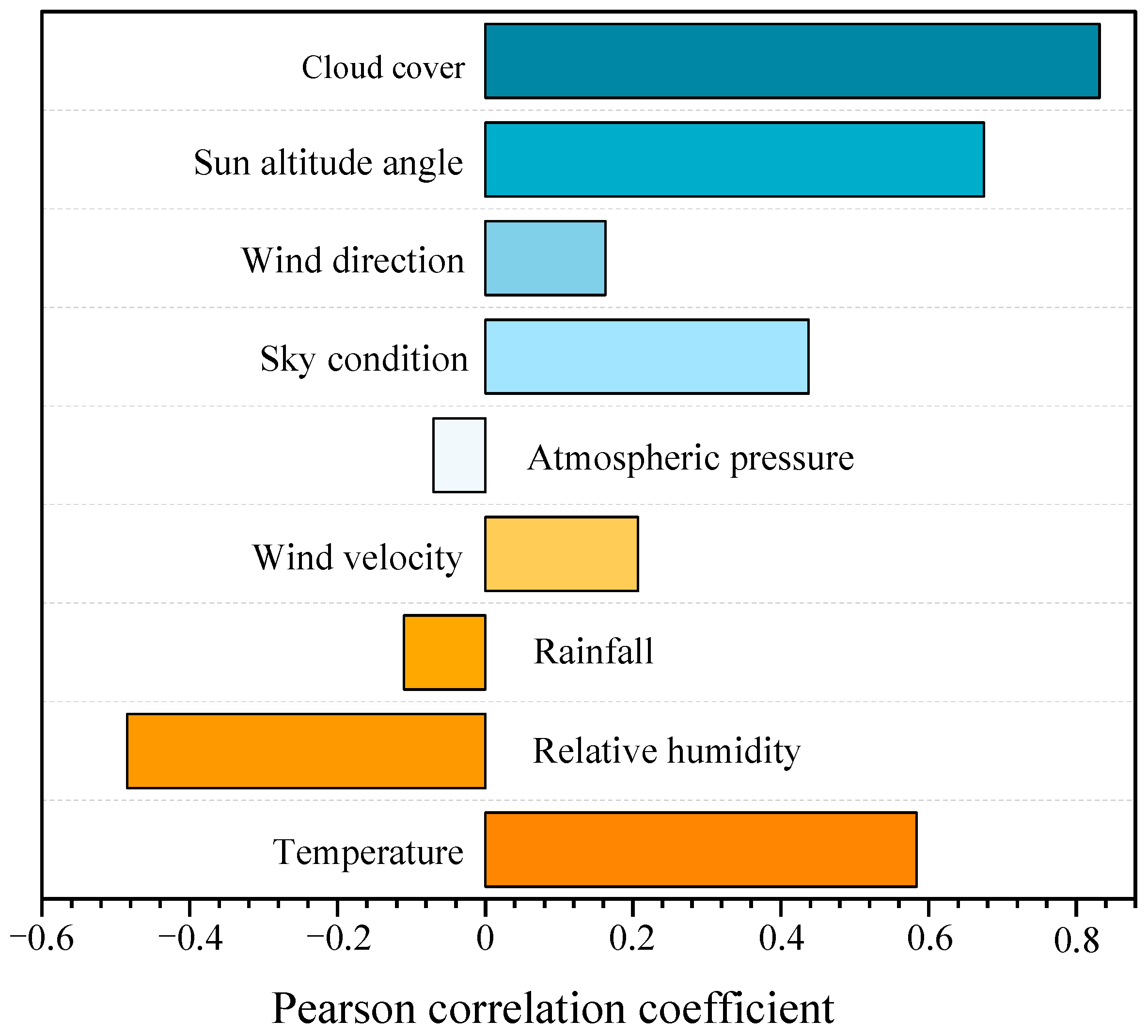
2.3.1. Correlation Analysis Between Meteorological Parameters and Daylight Illuminance

This section primarily analyzes the impact of common meteorological factors on daylight illuminance. As is well known, excessive input factors not only increase the complexity of predictions but also lead to the problem of information redundancy. On the other hand, too few data points may result in the omission of important information, thereby reducing the accuracy of the prediction model. Therefore, when selecting meteorological factors, it is essential to comprehensively extract useful information from the current dataset to avoid introducing meteorological factors that are weakly correlated with daylight illuminance prediction. In summary, an effective method is needed to quantitatively analyze the correlation between daylight illuminance and meteorological data.

The Pearson correlation coefficient can accurately measure the degree of association between multiple variables and provide deeper insight into their interactions. The coefficient ranges from −1 to 1, with values closer to 1 indicating a strong positive correlation between variables. By analyzing the relationships and interactions between variables, it helps to more accurately predict future trends. When the correlation coefficient between two variables approaches −1, it indicates a negative correlation, while a coefficient approaching 0 suggests no significant linear correlation. The Pearson correlation coefficient not only enhances the understanding of the relationship between two variables but also effectively reduces the interference caused by differences in the dimensionality of feature variables, providing more precise data support and significantly reducing the time cost of the research. The formula for calculating the Pearson correlation coefficient used in correlation analysis is shown in Equation (5):

$$r={\displaystyle \frac{{\displaystyle \sum (X-\overline{X})(Y-\overline{Y})}}{\sqrt{{{\displaystyle \sum (X-\overline{X})}}^2}\sqrt{{\displaystyle \sum {(Y-\overline{Y})}^2}}}}$$

(5)

Here, $\overline{X}$ refers to the mean of $X$, and $\overline{Y}$ refers to the mean of $Y$.

The Pearson correlation coefficients between the nine meteorological parameters mentioned in the previous section and daylight illuminance are shown in Figure 3. It can be observed that only cloud cover and solar altitude angle have a strong correlation with daylight illuminance, while temperature, relative humidity, and weather type show moderate correlation, with humidity being negatively correlated. According to research in the related literature, parameters with a Pearson correlation coefficient greater than 0.3 with the prediction target are considered effective [34]. Since the solar altitude angle follows a similar variation pattern throughout the day and is not representative, it was excluded. Additionally, weather type may have high collinearity with other meteorological variables (such as cloud cover), and using them together as model inputs could lead to information redundancy, thus increasing model complexity and reducing prediction efficiency. Therefore, to improve the accuracy of daylight illuminance prediction and reduce the model complexity, the subsequent sections of this paper will select temperature, relative humidity, and cloud cover as input features.

2.3.2. Similarity Calculation Method

For daylight illuminance prediction, selecting an appropriate similarity calculation method is crucial. Grey Relational Analysis and Cosine Similarity are two commonly used similarity measurement methods that can quantify the similarity between the target period and historical periods from different perspectives. This study combines both methods to select similar moments.

In the similarity calculation, Grey Relational Analysis focuses on the similarity of dynamic change patterns, while Cosine Similarity emphasizes the overall directional similarity of feature vectors. For the daylight illuminance prediction task, these two methods can be used together: Grey Relational Analysis helps identify historical periods whose variation trends align with the target period, while Cosine Similarity further evaluates whether the overall feature directions are consistent. Given that the comprehensive relationship of multi-dimensional meteorological features significantly impacts the prediction results, Cosine Similarity is more precise in capturing the overall directional similarity of features. Therefore, it is given a higher weight 0.6. On the other hand, Grey Relational Analysis focuses on describing dynamic trends and effectively complements the similarity of feature change patterns, so it is assigned a weight of 0.4. This weight distribution enhances the accuracy and reliability of the similar period selection by considering both feature change trends and overall feature direction similarity from multiple dimensions. The combined formula is shown in Equation (6):

$$S_i=0.4R_{oi}+0.6D_{oi}$$

(6)

Here, $R_{oi}$ represents the Grey Relational Analysis, $D_{oi}$ represents the Cosine Similarity, and $S_i$ represents the similarity index obtained by combining the Grey Relational Analysis and Cosine Similarity. The weights are 0.4 and 0.6, respectively.

When performing similarity analysis between the meteorological data (temperature, relative humidity, cloud cover) of the target moment and historical meteorological data, the correlation analysis results indicate that cloud cover has the highest correlation with daylight illuminance, followed by temperature, while relative humidity has the lowest correlation. Therefore, when calculating the final similarity, the weights for each feature need to be set appropriately based on their correlation with daylight illuminance. Specifically, based on the correlation analysis results, the weights for cloud cover, temperature, and relative humidity are set as 0.6, 0.3, and 0.1, respectively. This ensures that the contribution of each feature to daylight illuminance prediction is more accurately reflected. The final similarity calculation formula is as follows in Equation (7):

$$S_{Final}=0.6S_{\mathrm{C}}+0.3S_{\mathrm{T}}+0.1S_{\mathrm{RH}}$$

(7)

Here, $S_C$ represents the similarity of cloud cover, $S_T$ represents the similarity of temperature, and $S_{RH}$ represents the similarity of relative humidity. The weights are 0.6, 0.3, and 0.1, respectively. $S_{Final}$ represents the similarity of cloud cover, temperature, and relative humidity, as well as the final similarity obtained by combining these three similarities.

In each Meteorological Analog Instant, only the meteorological feature data of the target moment, along with the data of the previous and next moments, are selected to form an input dataset consisting of three consecutive time points. This method focuses on the local feature changes of the target moment, enabling it to more effectively capture the dynamic influence of adjacent moments on the target moment, while avoiding the interference of irrelevant information from the complete dataset.

2.3.3. Establishment of Meteorological Analog Intervals

The establishment process of Meteorological Analog Intervals is the key to implementing the similarity analysis method, directly affecting the accuracy of the selection results and the prediction performance. This section will design a standardized process for establishing Meteorological Analog Intervals, ensuring efficient and standardized support for the hourly prediction model of daylight illuminance. The flowchart for constructing the similar periods is shown in Figure 4. First, the data are preprocessed according to the data processing method in Section 2.1. The processed data are then divided into transitional seasons, summer, and winter. Afterward, a correlation analysis is conducted, and temperature, cloud cover, and relative humidity, which have a high correlation with daylight illuminance, are selected as input parameters. The similarity of these parameters is then calculated with historical meteorological data, and historical data with a comprehensive similarity greater than 0.6 are chosen as Meteorological Analog Instants. Finally, the Meteorological Analog Intervals are selected by including one time point before and after the Meteorological Analog Instants. In this context, $A_t$ represents the Meteorological Analog Instant, while $A_{t-1}$ and $A_{t+1}$ represent the time points before and after the Meteorological Analog Instant, respectively.

The specific process is as follows:

(1)

Date division and dataset construction:

Based on seasonal characteristics, historical dates are divided into the yransitional season, summer, and winter, and separate datasets $A$, $B$, and $C$ are constructed accordingly. Each dataset includes features $W$, including temperature, humidity, cloud cover, and daylight illuminance.

(2)

Feature normalization:

The features for each day in the historical data are normalized. Daylight illuminance, temperature, humidity, and cloud cover are normalized to the range [0, 1], eliminating the influence of different units among the indicators.

(3)

Moment splitting:

The dataset is split into moments based on the hourly unit. For example, in Dataset $A$ (transitional season)—the same applies for Dataset $B$ (summer season) and Dataset $C$ (winter season)—the data is split into $n$ moments, creating datasets A₁, A₂, …, A_n.

(4)

Selection of Meteorological Analog Instants:

Using similarity metrics, the meteorological feature values $W$ of the target moment are taken as inputs to perform similarity analysis with the corresponding historical moments $A_t$. The historical moments that have a similarity score greater than 0.6 with the target moment’s overall meteorological conditions are selected as meteorological analog instants.

(5)

Establishment of Meteorological Analog Intervals:

The selected meteorological analog instant $A_t$ and its adjacent moments $A_{t-1}$ and $A_{t+1}$ are extracted to form the final input dataset. This helps avoid interference from redundant information and improves prediction accuracy.

3. Daylight Illuminance Prediction Model

This chapter will design an hourly daylight illuminance prediction method that combines the Meteorological Analog Interval analysis method proposed in the previous chapter with a deep learning model. Since a single deep learning model may have difficulty fully capturing the features when dealing with complex time-series problems, this chapter introduces a hybrid deep learning model that integrates the Temporal Convolutional Network (TCN), Transformer, and Bidirectional Long Short-Term Memory Network (BILSTM). Compared to a single model, this multi-module fusion structure can comprehensively extract both short-term and long-term dependency features from the time series, capturing global and local temporal correlations. As a result, it further improves the prediction accuracy of the model.

3.1. Model Structure and Prediction Process

This chapter proposes a daylight illuminance prediction model that combines Meteorological Analog Interval analysis with deep learning, aiming to address the shortcomings of single deep learning algorithms in handling complex time-series forecasting tasks. Figure 5 shows the overall prediction process flowchart. The specific process is as follows: First, the data are preprocessed according to the data processing method in Section 2.1. The processed data are then subjected to correlation analysis and similarity calculation. Using relative humidity (RH), temperature (T), and cloud cover (C), the Meteorological Analog Instants are determined, which are further used to define the Meteorological Analog Intervals. The data from the similar intervals are then input into the TCN (Temporal Convolutional Network) module, which captures key features of the target moment and surrounding moments through convolution operations, modeling the temporal dependencies. The data processed by the TCN module are then fed into the Transformer module. The Transformer module uses the self-attention mechanism to capture the dynamic relationships between the target moment and its surrounding moments, analyzing the impact of meteorological features on daylight illuminance. Finally, the processed data are input into the BILSTM (Bidirectional Long Short-Term Memory) module. The BILSTM module processes the data of the target moment and its surrounding moments both forward and backward, completing the final daylight illuminance prediction task. The performance of the proposed model is then analyzed through evaluation metrics.

The model structure is composed of two main parts: the Meteorological Analog Interval Analysis part and the Deep Learning Prediction part, where the deep learning prediction part further includes the TCN module, Transformer module, and BILSTM module. Each part performs specific tasks in the overall prediction process:

(1)

Meteorological Analog Interval analysis:

Through selecting historical moments with similar meteorological features (such as temperature, humidity, cloud cover, etc.) to the target moment, and further constructing meteorological analog intervals, this step reduces data redundancy and noise interference, providing more representative and high-quality input data.

(2)

Temporal Convolutional Network (TCN) module:

The TCN focuses on extracting local temporal features. By using convolution operations, it captures the key features of the target moment and its adjacent moments, modeling the time dependencies. Its parallel computation capability ensures efficient processing, while the causal convolution structure prevents future information leakage.

(3)

Transformer module:

The Transformer captures the dynamic relationships between the target moment and its adjacent moments through the self-attention mechanism, analyzing the impact of meteorological features on daylight illuminance. Its ability to efficiently handle short time series preserves complex time-dependency modeling.

(4)

Bidirectional Long Short-Term Memory Network (BILSTM) module:

The BILSTM processes the target moment and its adjacent moments in both forward and backward directions, considering bidirectional constraints to improve prediction accuracy. Its gating mechanism optimizes feature selection and extracts the most important information from short time-series data.

3.2. CSP Site Selection Framework Based on MCDM and GIS

The specific steps of the model operation are as follows:

(1)

Data Preprocessing and Meteorological Analog Interval Selection:

The raw data are cleaned by handling missing values and outliers. Based on the characteristics of the target moment, historical data with a comprehensive similarity score greater than 0.6 are selected as Meteorological Analog Instants. These selected moments are further used to construct the Meteorological Analog Interval, ensuring data reliability and improving prediction performance.

(2)

Model Training:

The filtered data are input into the TCN module to extract short-term and long-term dependency features. Then, the features are passed to the Transformer module, where the self-attention mechanism learns global dependencies. Next, the BILSTM module captures the dynamic features of the time-series data using its bidirectional structure, ultimately generating the predicted result.

(3)

Model Evaluation:

The model’s prediction performance is evaluated using metrics such as RMSE and MAE to comprehensively assess the model’s prediction accuracy and robustness.

3.3. Results

In this chapter, the experiments were conducted using a dataset of Meteorological Analog Instants (MAIT) combined with the TCN-Transformer-BILSTM technique, while other models were based on the Meteorological Analog Interval (MAIL) dataset.

To improve the conciseness and logical clarity of the expression, the experiments and analysis in this section will adopt this abbreviation method. For example, the model based on Meteorological Analog Interval analysis using TCN-Transformer-BILSTM can be abbreviated as MAIL-T-TF-BILSTM.

The experiments were conducted using data collected in Xi’an. To more intuitively demonstrate the performance of the model, a total of 12 days were randomly selected from the following categories: transitional season, summer, and winter, under both optimal daylight condition and suboptimal daylight condition.

Figure 6, Figure 7 and Figure 8, respectively, show the prediction results of different models under optimal daylight condition and suboptimal daylight condition for the transitional season, summer, and winter. Figure 9 presents the overall error of the proposed model across different seasons under both optimal and suboptimal daylight conditions.

Figure 6 shows the performance of the models under transitional season daylight conditions. It is evident that, under optimal daylight conditions, all models perform relatively well, with prediction curves aligning closely with the actual illuminance data. The TCN-Transformer-BILSTM hybrid model, in particular, demonstrates superior fitting accuracy, effectively capturing the trend in illuminance changes. Figure 7 illustrates the results for the summer season, where the TCN-Transformer-BILSTM model again delivers the best prediction accuracy compared to the other models. However, under suboptimal conditions, where the weather fluctuates more, prediction errors increase, especially during periods with rapid changes in daylight illuminance. Figure 8 shows the results for the winter season. Similar to the summer season, the TCN-Transformer-BILSTM model outperforms the other models in terms of robustness, handling the complex environmental fluctuations typically seen during winter. Even under suboptimal conditions, this model still demonstrates good prediction performance.

Figure 9 summarizes the overall error of the proposed model across different seasons and daylight conditions. The results confirm that the TCN-Transformer-BILSTM model excels in minimizing error across both optimal and suboptimal daylight conditions, particularly during the winter season, where daylight illuminance tends to fluctuate more. Even under such conditions, the model still shows good prediction performance.

However, under suboptimal daylight condition, due to more significant fluctuations in illuminance, the prediction errors of the models increase notably, especially during periods of frequent illuminance changes (such as from 10:00 AM to 2:00 PM). Despite this, the hybrid model TCN-Transformer-BILSTM still demonstrates stronger adaptability and stability compared to the other models, providing relatively optimal prediction results under complex weather conditions. This further indicates that this model has greater potential and application value in handling the complex task of daylight illuminance prediction.

Table 4. Performance metrics of different models under optimal daylight condition for different seasons.

Season	Model	RMSE	MAE	MAPE (%)
transitional season	TCN-Trans-BILSTM	2001.32	1543.18	19.85
	TCN-BILSTM	2349.83	1849.79	23.22
	Trans-BILSTM	2417.93	1948.15	24.43
	BILSTM	2573.52	2157.52	26.57
	MAIT-T-TF-BILSTM	2481.43	2024.35	25.13
Summer season	TCN-Trans-BILSTM	1625.83	1487.70	16.99
	TCN-BILSTM	1957.43	1651.78	21.82
	Trans-BILSTM	2001.35	1704.39	22.44
	BILSTM	2145.52	1825.23	24.54
	MAIT-T-TF-BILSTM	2073.82	1753.93	23.22
Winter season	TCN-Trans-BILSTM	2274.01	1860.02	22.06
	TCN-BILSTM	2621.40	2095.78	25.76
	Trans-BILSTM	2695.21	2695.21	26.88
	BILSTM	2846.01	2244.59	28.36
	MAIT-T-TF-BILSTM	2763.82	2198.75	27.63

and

Table 5. Performance metrics of different models under suboptimal daylight condition for different seasons.

Season	Model	RMSE	MAE	MAPE (%)
Transitional season	TCN-Trans-BILSTM	3180.13	2907.63	29.22
	TCN-BILSTM	3745.81	3458.93	32.47
	Trans-BILSTM	3789.46	3498.01	33.88
	BILSTM	4116.58	3824.48	36.54
	MAIT-T-TF-BILSTM	3958.21	3701.59	35.27
Summer season	TCN-Trans-BILSTM	2581.45	2041.68	24.99
	TCN-BILSTM	2895.31	2432.42	28.14
	Trans-BILSTM	2937.47	2475.02	28.84
	BILSTM	3132.75	2644.23	30.47
	MAIT-T-TF-BILSTM	3054.67	2592.31	29.87
Winter season	TCN-Trans-BILSTM	2583.84	2137.47	25.03
	TCN-BILSTM	2915.83	2580.93	30.02
	Trans-BILSTM	2880.54	2537.82	29.42
	BILSTM	3098.25	2733.59	31.37
	MAIT-T-TF-BILSTM	3032.15	2671.43	31.11

show the performance metrics of different models under optimal daylight condition and suboptimal daylight condition for different seasons. Table 4 presents the performance metrics of different models under optimal daylight conditions for the transitional season, summer, and winter. The results indicate that the TCN-Transformer-BILSTM model consistently achieves the lowest RMSE and MAE values, showcasing its superior ability to predict daylight illuminance accurately. Table 5 presents the performance metrics of these models under suboptimal daylight conditions. Even in less-than-ideal conditions, the TCN-Transformer-BILSTM model maintains the lowest MAPE, proving its robustness and accuracy. Notably, under summer suboptimal conditions, the TCN-Transformer-BILSTM model exhibits a significantly lower MAPE compared to the other models, highlighting its stronger adaptability to fluctuating weather conditions.

From an overall perspective, the models perform better under optimal daylight condition, mainly because the illuminance intensity is more stable, allowing the models to better capture its trend, resulting in lower errors. Specific to model performance, from the perspective of MAPE, TCN-Trans-BILSTM shows the lowest error across all seasons and weather conditions. For example, under summer optimal daylight condition, TCN-Trans-BILSTM has a MAPE of only 16.989%, which is 4.84 percentage points lower than the second-best model TCN-BILSTM (MAPE of 21.82%). In suboptimal daylight condition, TCN-Trans-BILSTM also performs excellently. For instance, under winter suboptimal daylight condition, its MAPE is 22.06%, which is 4.81 percentage points lower than Trans-BILSTM’s MAPE of 26.88%. This indicates that TCN-Trans-BILSTM, after the selection of Meteorological Analog Intervals, has a significantly better ability to capture illuminance fluctuations under complex weather conditions compared to other models.

Other models, such as TCN-BILSTM and Trans-BILSTM, perform well under optimal daylight conditions but show a significant increase in error under suboptimal daylight conditions. For example, under transitional season suboptimal daylight condition, TCN-BILSTM has a MAPE of 25.76%, which is 3.33 percentage points higher than TCN-Trans-BILSTM’s MAPE of 22.44%.

The simple model BILSTM, although more computationally efficient, exhibits weaker performance under complex weather conditions. For instance, in winter suboptimal daylight condition, BILSTM has a MAPE of 28.36%, which is 6.30 percentage points higher than TCN-Trans-BILSTM, further indicating that its ability to adapt to complex illuminance fluctuations is limited.

It is worth noting that the dataset after Meteorological Analog Interval grouping significantly improves the model performance. For instance, after grouping the data by Meteorological Analog Intervals, the TCN-Trans-BILSTM model consistently shows a MAPE that is significantly lower than that of other models that did not undergo the selection process, demonstrating stronger robustness and broader applicability. This advantage is especially prominent under suboptimal daylight conditions. Regardless of the season—whether transitional, summer, or winter—the error reduction for TCN-Trans-BILSTM is consistently between 4–6 percentage points, further highlighting the optimization effect that fine-tuning the data selection process has on the performance of daylight illuminance prediction models.

In summary, TCN-Trans-BILSTM is the best-performing model in this study. After applying the Meteorological Analog Interval selection, it exhibits lower errors, stronger robustness, and broader applicability. Other models, such as TCN-BILSTM and Trans-BILSTM, also show good performance under certain specific conditions but have slightly weaker adaptability to complex weather. As for BILSTM, despite its higher computational efficiency, its adaptability to complex environments still needs improvement.

Therefore, based on different application needs, the TCN-Trans-BILSTM model, after Meteorological Analog Interval selection, is the optimal choice for scenarios requiring high accuracy and robustness. Other models can be flexibly used depending on computational resources and practical scenario requirements. This study further verifies the significant role that data grouped by Meteorological Analog Intervals play in improving model prediction accuracy.

4. Conclusions

This study addresses the challenges of hourly daylight illuminance prediction, such as large fluctuations due to weather conditions, high data noise, and complex nonlinear features, by proposing an innovative solution that combines Meteorological Analog Interval analysis with the TCN-Transformer-BILSTM hybrid architecture. The Meteorological Analog Interval analysis first uses gray correlation degree and cosine similarity to select historical data that most closely match the meteorological conditions and time attributes of the target moment. It then constructs Meteorological Analog Intervals by selecting the previous and subsequent moments of the similar instants, focusing on the local dynamic changes before and after the target moment. This strategy significantly reduces the randomness and noise interference in the data, strengthens the correlation and representativeness of the input data, and demonstrates excellent stability and robustness, especially under complex meteorological conditions.

Moreover, the hybrid model, by integrating the advantages of TCN, Transformer, and BILSTM, overcomes the limitations of a single model in capturing both long-term and short-term dependencies as well as global nonlinear features in time series. Experimental results show that the proposed model performs optimally under ideal weather conditions, achieving the lowest RMSE and MAE, with values of 1625.83 Lux and 1487.70 Lux, respectively. Even under suboptimal weather conditions, the model maintains strong adaptability, with prediction errors significantly lower than those of single models and traditional methods. The experimental results also reveal that predictions in the summer perform better than in the transitional season and winter, possibly due to the region’s abundant summer sunlight and predominantly clear weather.

This study successfully addresses the difficulties in nonlinear modeling caused by weather fluctuations and the insufficient prediction accuracy in daylight illuminance forecasting. The proposed method offers a scalable, high-precision solution for hourly daylight illuminance prediction and shows broad application potential in fields such as energy-efficient building design, smart lighting system optimization, and dynamic energy management. Future work will further optimize the Meteorological Analog Interval selection strategy, explore real-time adaptive mechanisms, and incorporate more environmental variables to enhance the model’s dynamic adaptability and robustness, thus providing new theoretical and practical support for the sustainable development of intelligent energy systems.

References

1. Ohene, E.; Chan, A.P.; Darko, A. Review of global research advances towards net-zero emissions buildings. Energy Build. 2022, 266, 112142. [Google Scholar] [CrossRef]
2. Dong, X. Research and Application of the Sustainable Architectural Design Theory. In Proceedings of the 3rd International Conference on Architecture: Heritage, Traditions and Innovations (AHTI 2021), Moscow, Russia, 9–10 March 2021; Atlantis Press: Dordrecht, The Netherlands, 2021; pp. 72–78. [Google Scholar]
3. Wang, H.; Lu, W.; Wu, Z.; Zhang, G. Parametric analysis of applying PCM wallboards for energy saving in high-rise lightweight buildings in Shanghai. Renew. Energy 2020, 145, 52–64. [Google Scholar] [CrossRef]
4. Li, D.H.; Lam, T.N.; Chan, W.W.; Mak, A.H. Energy and cost analysis of semi-transparent photovoltaic in office buildings. Appl. Energy 2009, 86, 722–729. [Google Scholar] [CrossRef]
5. Ghimire, S.; Deo, R.C.; Raj, N.; Mi, J. Deep solar radiation forecasting with convolutional neural network and long short-term memory network algorithms. Appl. Energy 2019, 253, 113541. [Google Scholar] [CrossRef]
6. Bhatia, A.; Sangireddy, S.A.R.; Garg, V. An approach to calculate the equivalent solar heat gain coefficient of glass windows with fixed and dynamic shading in tropical climates. J. Build. Eng. 2019, 22, 90–100. [Google Scholar] [CrossRef]
7. Vardakas, J.S.; Zorba, N.; Verikoukis, C.V. A survey on demand response programs in smart grids: Pricing methods and optimization algorithms. IEEE Commun. Surv. Tutor. 2014, 17, 152–178. [Google Scholar] [CrossRef]
8. Mead, M.N. Benefits of Sunlight: A Bright Spot for Human Health; National Institute of Environmental Health Sciences: Durham, NC, USA, 2008.
9. Lüthi, S.; Wüstenhagen, R. The price of policy risk—Empirical insights from choice experiments with European photovoltaic project developers. Energy Econ. 2012, 34, 1001–1011. [Google Scholar] [CrossRef]
10. Cao, X.; Dai, X.; Liu, J. Building energy-consumption status worldwide and the state-of-the-art technologies for zero-energy buildings during the past decade. Energy Build. 2016, 128, 198–213. [Google Scholar] [CrossRef]
11. Fumo, N.; Biswas, M.A.R. Regression analysis for prediction of residential energy consumption. Renew. Sustain. Energy Rev. 2015, 47, 332–343. [Google Scholar] [CrossRef]
12. Holt, C.C. Forecasting seasonals and trends by exponentially weighted moving averages. Int. J. Forecast. 2004, 20, 5–10. [Google Scholar] [CrossRef]
13. Liao, Z.; Gai, N.; Stansby, P.; Li, G. Linear non-causal optimal control of an attenuator type wave energy converter m4. IEEE Trans. Sustain. Energy 2019, 11, 1278–1286. [Google Scholar] [CrossRef]
14. Sen, P.; Roy, M.; Pal, P. Application of ARIMA for forecasting energy consumption and GHG emission: A case study of an Indian pig iron manufacturing organization. Energy 2016, 116, 1031–1038. [Google Scholar] [CrossRef]
15. Sina, A.; Kaur, D. Short term load forecasting model based on kernel-support vector regression with social spider optimization algorithm. J. Electr. Eng. Technol. 2020, 15, 393–402. [Google Scholar] [CrossRef]
16. Hu, J.; Zheng, W.; Zhang, S.; Li, H.; Liu, Z.; Zhang, G.; Yang, X. Thermal load prediction and operation optimization of office building with a zone-level artificial neural network and rule-based control. Appl. Energy 2021, 300, 117429. [Google Scholar] [CrossRef]
17. Javed, F.; Arshad, N.; Wallin, F.; Vassileva, I.; Dahlquist, E. Forecasting for demand response in smart grids: An analysis on use of anthropologic and structural data and short term multiple loads forecasting. Appl. Energy 2012, 96, 150–160. [Google Scholar] [CrossRef]
18. Liu, X.; Yu, J.; Zhao, A.; Jing, W.; Mi, L. A hybrid WOA-SVM based on CI for improving the accuracy of shopping mall air conditioning system energy consumption prediction. Energy Build. 2023, 294, 113186. [Google Scholar] [CrossRef]
19. Mellit, A.; Pavan, A.M. A 24-h forecast of solar irradiance using artificial neural network: Application for performance prediction of a grid-connected PV plant at Trieste, Italy. Sol. Energy 2010, 84, 807–821. [Google Scholar] [CrossRef]
20. Sherstinsky, A. Fundamentals of recurrent neural network (RNN) and long short-term memory (LSTM) network. Phys. D Nonlinear Phenom. 2020, 404, 132306. [Google Scholar] [CrossRef]
21. Hochreiter, S.; Schmidhuber, J. Long short-term memory. Neural Comput. 1997, 9, 1735–1780. [Google Scholar] [CrossRef]
22. Yu, Z.; Moirangthem, D.S.; Lee, M. Continuous timescale long-short term memory neural network for human intent understanding. Front. Neurorobot. 2017, 11, 42. [Google Scholar] [CrossRef]
23. Zarzycki, K.; Ławryńczuk, M. Advanced predictive control for GRU and LSTM networks. Inf. Sci. 2022, 616, 229–254. [Google Scholar] [CrossRef]
24. Huang, X.; Zhang, C.; Li, Q.; Tai, Y.; Gao, B.; Shi, J. A Comparison of Hour-Ahead Solar Irradiance Forecasting Models Based on LSTM Network. Math. Probl. Eng. 2020, 2020, 4251517. [Google Scholar] [CrossRef]
25. Atef, S.; Eltawil, A.B. Assessment of stacked unidirectional and bidirectional long short-term memory networks for electricity load forecasting. Electr. Power Syst. Res. 2020, 187, 106489. [Google Scholar] [CrossRef]
26. Michael, N.E.; Bansal, R.C.; Ismail, A.A.A.; Elnady, A.; Hasan, S. A cohesive structure of Bi-directional long-short-term memory (BiLSTM)-GRU for predicting hourly solar radiation. Renew. Energy 2024, 222, 119943. [Google Scholar] [CrossRef]
27. Li, Z.; Shi, H.; Yang, X.; Tang, H. Investigating the nonlinear relationship between surface solar radiation and its influencing factors in North China Plain using interpretable machine learning. Atmos. Res. 2022, 280, 106406. [Google Scholar] [CrossRef]
28. Limouni, T.; Yaagoubi, R.; Bouziane, K.; Guissi, K.; Baali, E.H. Accurate one step and multistep forecasting of very short-term PV power using LSTM-TCN model. Renew. Energy 2023, 205, 1010–1024. [Google Scholar] [CrossRef]
29. Pang, H.; Gao, J.; Du, Y. A short-term load probability density prediction based on quantile regression of time convolution network. Power Syst. Technol. 2020, 44, 1343–1350. [Google Scholar]
30. Liu, H.; Zhou, Y.; Luo, Q.; Huang, H.; Wei, X. Prediction of photovoltaic power output based on similar day analysis using RBF neural network with adaptive black widow optimization algorithm and K-means clustering. Front. Energy Res. 2022, 10, 990018. [Google Scholar] [CrossRef]
31. Janković, Z.; Selakov, A.; Bekut, D.; Đorđević, M. Day similarity metric model for short-term load forecasting supported by PSO and artificial neural network. Electr. Eng. 2021, 103, 2973–2988. [Google Scholar] [CrossRef]
32. Zeng, W.; Li, J.; Sun, C.; Cao, L.; Tang, X.; Shu, S.; Zheng, J. Ultra short-term power load forecasting based on similar day clustering and ensemble empirical mode decomposition. Energies 2023, 16, 1989. [Google Scholar] [CrossRef]
33. Kim, D.; Lee, D.; Nam, H.; Joo, S.-K. Short-term load forecasting for commercial building using convolutional neural network (CNN) and long short-term memory (LSTM) network with similar day selection model. J. Electr. Eng. Technol. 2023, 18, 4001–4009. [Google Scholar] [CrossRef]
34. Voyant, C.; Muselli, M.; Paoli, C.; Nivet, M.-L. Optimization of an artificial neural network dedicated to the multivariate forecasting of daily global radiation. Energy 2011, 36, 348–359. [Google Scholar] [CrossRef]
Figure 1. The methodological framework of this study.
Sustainability 17 04914 g001
Figure 2. Graph of daily variation curves for different daylight illuminance.
Sustainability 17 04914 g002
Figure 3. Pearson correlation coefficients between different meteorological parameters and daylight illuminance.
Sustainability 17 04914 g003
Figure 4. Flowchart for constructing Meteorological Analog Intervals.
Sustainability 17 04914 g004
Figure 5. Structure diagram of the daylight illuminance prediction model.
Sustainability 17 04914 g005
Figure 6. Prediction results of different models under transitional season optimal daylight condition and suboptimal daylight condition.
Sustainability 17 04914 g006
Figure 7. Prediction results of different models under summer optimal daylight condition and suboptimal daylight condition.
Sustainability 17 04914 g007
Figure 8. Prediction results of different models under winter optimal daylight condition and suboptimal daylight condition.
Sustainability 17 04914 g008
Figure 9. Errors of the TCN-Trans-BILSTM model based on Meteorological Analog Interval in different conditions.
Sustainability 17 04914 g009