Optimizing Subsurface Drainage Pipe Layout Parameters in Southern Xinjiang’s Saline–Alkali Soils: Impacts on Soil Salinity Dynamics and Oil Sunflower Growth Performance

Abstract

This study addresses secondary soil salinization driven by shallow groundwater in the Yanqi Basin of southern Xinjiang, focusing on subsurface drainage system (SDS) optimization for salt regulation and oil sunflower productivity improvement in severe saline–alkali soils. Through controlled field experiments conducted (May–October 2024), we evaluated five SDS configurations: control (CK, no drainage) and four drain spacing/depth combinations (20/40 m × 1.2/1.5 m). Comprehensive monitoring revealed distinct spatiotemporal patterns, with surface salt accumulation (0–20 cm: 18.59–32.94 g·kg⁻¹) consistently exceeding subsurface levels (>20–200 cm: 6.79–17.69 g·kg⁻¹). The A3 configuration (20 m spacing, 1.5 m depth) demonstrated optimal root zone desalination (0–60 cm: 14.118 g·kg⁻¹), achieving 39.02% salinity reduction compared to CK (p < 0.01). Multivariate analysis revealed strong depth-dependent inverse correlations between groundwater level and soil salinity (R² = 0.529–0.919), with burial depth exhibiting 1.7-fold greater regulatory influence than spacing parameters (p < 0.01). Crop performance followed salinity gradients (A3 > A1 > A4 > A2 > CK), showing significant yield improvements across all SDS treatments versus CK (p < 0.05). Multi-criteria optimization integrating TOPSIS modeling and genetic algorithms identified A3 as the Pareto-optimal solution. The optimized configuration (20 m spacing, 1.5 m depth) effectively stabilized aquifer dynamics, reduced topsoil salinization (0–60 cm), and enhanced crop adaptability in silt loam soils. This research establishes an engineering framework for sustainable saline–alkali soil remediation in arid basin agroecosystems, providing critical insights for water–soil management in similar ecoregions.

1. Introduction

Soil serves as an indispensable natural resource for agricultural production and a critical foundation for both human society and the biosphere [1]. Soil salinization predominantly occurs in arid climates characterized by high evaporation rates, limited precipitation, elevated groundwater tables, and hypersaline conditions [2]. Currently, saline-affected soils are distributed across over 100 countries worldwide, covering approximately 1.1 × 10⁹ hm². Furthermore, the global salinization severity continues to escalate, particularly in vulnerable ecosystems [3]. This phenomenon is prevalent in critical agricultural zones including California’s Central Valley (USA), the Indo-Gangetic Plain (India), Dutch coastal lowlands, Egypt’s Nile Delta, and Northwest China. Salinization reduces crop yields by up to 18%, severely threatening agricultural sustainability and global food production systems [4]. A comprehensive understanding of salinization spatial patterns and driving mechanisms has become imperative for tackling environmental degradation and ensuring food security.

In arid regions, soil salinity dynamics are primarily governed by pedological characteristics, groundwater table depth, groundwater mineralization, and climatic factors [5,6]. Empirical studies reveal significant climate–salinity correlations: enhanced evapotranspiration intensifies salinization, while elevated precipitation reduces soil salinity in well-drained areas [7]. Shallow groundwater tables (<2 m) enable upward salt transport to the soil surface through capillary rise, directly inducing secondary salinization. This mechanism becomes particularly critical in irrigated agricultural zones where shallow water tables synergize with high evaporation rates to drive topsoil salt accumulation. Current remediation strategies employ integrated approaches: physical (deep tillage), chemical (flue gas desulfurization/phosphogypsum amendments), hydrological (subsurface drainage systems), and biological (halophyte cultivation). In Xinjiang’s agricultural irrigation districts, annual evaporation exceeds precipitation, compounded by prevalent shallow groundwater tables. As an effective measure for saline–alkali soil remediation, subsurface pipe drainage regulates groundwater tables, mitigates capillary-driven evaporation, and reduces soil salinity while improving soil physicochemical properties. Soluble salts are leached into groundwater and discharged via subsurface pipes [8,9].

Although research on subsurface drainage pipes for saline–alkali soil remediation has been extensive, significant variations in the ecological adaptability of their configuration parameters remain evident. Jafari-Talukolaee [10] investigated subsurface drainage systems under various depth and spacing configurations through continuous monitoring of groundwater levels, drainage discharge, and crop yields. Their research proposed optimal installation parameters for northern Iran, recommending a pipe spacing of 30 m with a burial depth of 0.9 m. Zhang [11] found that narrower pipe spacing and greater depth improved drainage and salt removal efficiency, while reducing soil water storage during drainage periods and salt accumulation during non-drainage phases. Field trials by Zhu [12], Yang [13], and Shi [14] in southern Xinjiang demonstrated optimal desalination efficiency with subsurface pipes at depths of 0.8–1.5 m and spacings of 8–10 m. Wen [15] conducted field trials in Shawan employing drip irrigation leaching combined with subsurface drainage systems at 15 m spacing and variable burial depths (0.6, 1.0, and 1.4 m). Their results demonstrated superior saline–alkali soil remediation efficiency with 0.6 m burial depth compared to deeper configurations. These findings underscore the necessity of site-specific parameter optimization through field investigations and experimental studies. Given the substantial costs associated with field trials, numerical modeling has become an essential tool for cost-effective drainage system optimization. Hamed [16] simulated drainage using the HYDRUS-2D model, revealing reduced drainage rates with wider spacings, with the highest rate observed at 7.5 m spacing and 1 m depth. Qian [17] studied subsurface pipe leaching in arid regions, achieving a 36% desalination rate at 1.4 m depth and 8 m spacing. Qi [18] validated and simulated subsurface drainage systems using field-measured data from sunflower plots in the Hetao Irrigation District through DRAINMOD modeling. The study identified optimal local drainage parameters as 1.5 m burial depth with 20 m spacing. Conventional physical models (HYDRUS-2D) are predominantly employed to simulate soil water–salt dynamics, demonstrating robust performance in single-objective analyses such as salt accumulation prediction. In contrast, multi-objective genetic algorithms operate as optimization tools that identify Pareto-optimal solutions among conflicting objectives (e.g., economic efficiency vs. ecological conservation). These algorithms generate multiple trade-off scenarios through Pareto frontiers. The entropy weight TOPSIS (Technique for Order Preference by Similarity to Ideal Solution) methodology complements this approach by providing objective weight allocation, enabling systematic selection of optimal solutions from the Pareto set while mitigating inherent algorithmic limitations.

Mechanistic interactions between subsurface drainage configurations and salt accumulation dynamics across crop phenological stages. Quantitative linkages between groundwater table depth and salt redistribution patterns in arid irrigation districts. This study innovatively integrates a multi-objective genetic algorithm with TOPSIS decision modeling to construct 3D response surfaces elucidating the depth–spacing–salinity nexus. This approach overcomes the local optima traps inherent in conventional single-objective optimization frameworks. These findings establish a theoretical foundation for combating secondary salinization in the Yanqi Basin of southern Xinjiang, while providing a transferable methodological framework for saline soil amelioration in arid agroecosystems globally.

2. Materials and Methods

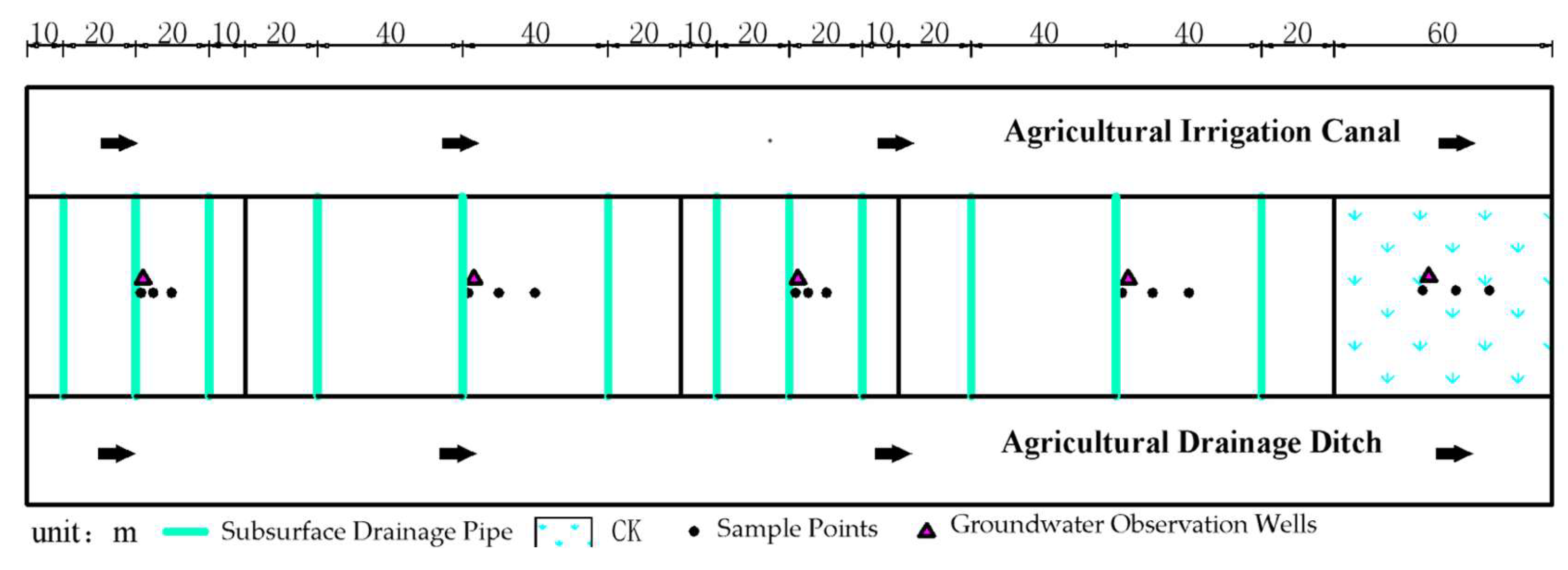
2.1. Site Description

The experimental site is located in Nong’erlian, 223rd Regiment of Hejing County, northwestern Yanqi Basin, southern Xinjiang (86°47′ E, 42°16′ N; elevation 1005.4 m). The region features a temperate continental climate with a north-high, south-low topography, characterized by sufficient sunlight, low precipitation, and high evaporation. Mean annual precipitation is 47.9 mm, evaporation is 2279.1 mm, and temperature is 8.7 °C (range: −30 °C to 37.2 °C). The frost-free period spans 195 days, with an annual sunshine duration of 3060.3 h and intense solar radiation due to high incident angles. Groundwater levels in the experimental area fluctuate seasonally and with irrigation, ranging from 1.6 to 2.4 m during the oil sunflower growing season. The site, classified as heavily saline–alkali, had been fallow for years until remediation began in 2023. All experimental plots exhibited a silt loam soil texture, with surface soil (0–20 cm) averaging ~25 g·kg⁻¹ salinity, meeting saline soil classification [19]. Studying the oil sunflower as the sole test crop, the soil types and physical properties are detailed in

Table 1. Soil physical properties in the experimental area.

Depth/cm	Bulk Density/(g·cm−3)	Total Porosity/%	Clay/%	Silt/%	Sand/%
0–20	1.59	40.30	15.70	62.01	22.29
20–40	1.54	39.06	15.69	61.12	23.19
40–60	1.47	40.14	14.43	59.39	26.18
60–80	1.53	38.30	14.27	58.50	27.23
80–100	1.62	40.65	13.06	53.06	33.88
100–120	1.59	38.70	12.31	52.97	34.72
120–140	1.55	51.26	11.61	52.04	36.35
140–160	1.61	44.24	10.00	44.99	45.01
160–180	1.61	45.46	9.32	43.78	46.90
180–200	1.62	46.00	9.01	42.37	48.62

.

2.2. Experimental Design

The experiment was conducted in a field measuring 420 m in length and 53 m in width. Three subsurface drainage pipes were installed in each experimental plot: the central pipe served as the monitoring and sampling conduit, while the two lateral pipes functioned as protective buffers. Each pipe, constructed from single-wall corrugated PVC material, measured 55 m in length with a diameter of 90 mm, a ring stiffness of 2.5 kN/m², a permeable area of 53 cm²/m, and a slope gradient of 0.1%. All pipes were connected to a shared agricultural drainage ditch at their termini to ensure unimpeded drainage (see Figure 1 for the experimental layout).

The experimental design incorporated two subsurface drainage pipe parameters: spacing and burial depth. These parameters were determined based on previous studies of subsurface drainage and salt leaching [20,21], as well as the determination of optimal subsurface drainage depth and spacing based on regional groundwater table depth, soil permeability, and engineering benefits. Each parameter was assigned two levels: spacing (20 m, 40 m) and burial depth (1.2 m, 1.5 m). Five treatments were established: A1 (1.2 m, 20 m), A2 (1.2 m, 40 m), A3 (1.5 m, 20 m), A4 (1.5 m, 40 m), and CK (no dark pipe), as detailed in

Table 2. Subsurface drainage system configuration in experimental plots.

Parameter	A1	A2	A3	A4	CK
Spacing/m	20	40	20	40	-
Depth/m	1.2	1.2	1.5	1.5
Area/m2	3180	6360	3180	6360	3180

.

2.3. Sample Determination and Processing

2.3.1. Soil Sample Treatment

Samples were taken 6 times after spring irrigation and before the whole growth period of winter irrigation, and the number of samples was 150. The sampling dates were May 15 (after spring irrigation), June 25 (seedling), July 24 (bud), August 15 (flowering), September 28 (mature), and October 25 (before winter irrigation). Triplicate soil sampling was systematically conducted across treatments A1–A4 and the control group (CK), with setup sampling points above the dark pipe, 0 spacing, 1/2 spacing, and 1/4 spacing following a stratified random design within experimental plots. For each sampling, 0–20, 20–40, 40–60, 60–80, 80–100, 100–120, 120–140, 140–160, 160–180, and 180–200 cm, 10 layers of soil samples were stratified for soil sampling and soil salt content.

Soil salt content: the conductivity of soil extract (EC_1:5) was determined by the digital display conductivity meter (DDS-307, Shanghai lightning magnetic, Shanghai, China), and the total soil salt content (TDS) was measured in the soil sample by the residue drying method [22]. The relationship curve between TDS and EC_1:5 in the test site can be expressed by Formula (1):

$$TDS=3.1479{EC}_{1:5}+0.0661(R^2=0.9977)$$

(1)

In the formula, TDS is the total salt content of soil, g·kg⁻¹; EC_1:5 is the conductivity of the soil extract with a water and soil mass ratio of 1:5, mS·cm⁻¹.

Soil salt deposition accumulation: The soil salinity is calculated by Formula (1) in layers. Since the initial salinity of each treatment layer is different after irrigation, the salt accumulation is calculated by Formula (2) in layers:

$$N=S_{i+1}-S_i$$

(2)

In the formula, N is the amount of salt accumulated, g·kg⁻¹; $S_i$ is the initial salt content of the soil, g·kg⁻¹; $S_{i+1}$ is the final salt content of the soil, g·kg⁻¹.

Groundwater level depth: Groundwater observation wells are set up in each community. The observation wells are PVC pipes with a length of 3.5 m and a diameter of 60 mm, which are vertically buried underground. The depth is 3.0 m. The underground part is drilled and wrapped with filter cloth, and groundwater observation meters (Xinjiang Agricultural University, Urumqi, China) are installed to monitor the data in real time and automatically record the observation data every hour.

The experimental site is located in an arid region, where annual evaporation far exceeds rainfall. The depth of groundwater is one of the key factors affecting soil salinization, and controlling the depth of groundwater is a crucial function of subsurface drainage. To investigate the relationship between groundwater depth and soil salinity, monthly groundwater depths at A1 to A4 were fitted against total soil salinity at 0–20 cm, 40–60 cm, 80–100 cm, and 120–140 cm soil layers. A fitting model was established, with its mathematical expression as shown in Formula (3):

$$\mathrm{y}=\mathrm{a}+\mathrm{b}\mathrm{h}$$

(3)

where y is the total salt content of the soil, g·kg⁻¹; h is the buried depth of groundwater, m; a and b are the pending coefficients.

2.3.2. Crop Growth Index

Plant height: 3 plants were randomly selected in each treatment area in each growth period and measured by tape.

Stem diameter: 3 plants were randomly selected in each treatment area in each crop growth period and measured by vernier caliper.

Flower head dry weight: 3 strains of oil sunflower were randomly selected for each treatment during crop maturity; the flower plates were cut with scissors, put into the oven for drying, and their dry weight was measured.

Dry 100-seed weight: 3 strains of oil sunflower were randomly selected for each treatment of the crop maturity for drying, and 1000 oil sunflower seeds were weighed.

2.4. Model

2.4.1. Multi-Objective Genetic Algorithm

Agricultural production systems require multi-objective optimization where objectives often extend beyond optimizing a single parameter to encompass holistic consideration of economic efficiency and ecological outcomes. These complex decision-making scenarios are formally classified as multi-objective optimization problems. The genetic algorithm (GA) represents a stochastic search methodology that emulates biological evolutionary mechanisms. Demonstrated through applications in engineering design, resource allocation, and environmental modeling, GAs exhibit superior capability in navigating high-dimensional, non-linear search spaces while maintaining robust adaptability across diverse problem domains [23].

Pareto: The Pareto front (or Pareto-optimal frontier) represents the set of all non-dominated solutions in multi-objective optimization, where no objective can be improved without degrading at least one other objective.

Goal 1 (maximum 100-seed dry weight):

$${\mathrm{f}}_1\left({\mathrm{x}}_1,{\mathrm{x}}_2\right)=-{\mathrm{F}}_{\mathrm{y}\mathrm{i}\mathrm{e}\mathrm{l}\mathrm{d}}\left({\mathrm{x}}_1,{\mathrm{x}}_2\right)$$

(4)

Goal 2 (Minimize salt accumulation):

$${\mathrm{f}}_2\left({\mathrm{x}}_1,{\mathrm{x}}_2\right)=-{\mathrm{F}}_{\mathrm{s}\mathrm{a}\mathrm{l}\mathrm{t}}\left({\mathrm{x}}_1,{\mathrm{x}}_2\right)$$

(5)

Formal description of optimization problem:

$${\mathrm{m}\mathrm{i}\mathrm{n}}_{\left({\mathrm{x}}_1,{\mathrm{x}}_2\right)}=\left[{\mathrm{f}}_1\left({\mathrm{x}}_1,{\mathrm{x}}_2\right),{\mathrm{f}}_2\left({\mathrm{x}}_1,{\mathrm{x}}_2\right)\right]$$

(6)

$${20\le \mathrm{x}}_1\le 40$$

(7)

$${1.2\le \mathrm{x}}_2\le 1.5$$

(8)

${\mathrm{x}}_1$ indicates the spacing of the dark pipe, m; ${\mathrm{x}}_2$ indicates the depth of the hidden pipe, m.

${\mathrm{F}}_{\mathrm{y}\mathrm{i}\mathrm{e}\mathrm{l}\mathrm{d}}\left({\mathrm{x}}_1,{\mathrm{x}}_2\right) \mathrm{a}\mathrm{n}\mathrm{d} {\mathrm{F}}_{\mathrm{s}\mathrm{a}\mathrm{l}\mathrm{t}}\left({\mathrm{x}}_1,{\mathrm{x}}_2\right)$ are interpolation functions based on experimental data: ${\mathrm{F}}_{\mathrm{y}\mathrm{i}\mathrm{e}\mathrm{l}\mathrm{d}}\left({\mathrm{x}}_1,{\mathrm{x}}_2\right)$ is a natural neighbor interpolation function for normalized dry grain weight, reflecting the positive effect of ${\mathrm{x}}_1$ and ${\mathrm{x}}_2$ on yield.

2.4.2. Entropy Weight TOPSIS

Construct an n by m evaluation matrix, where ${\mathrm{x}}_{\mathrm{i}\mathrm{j}}$ represents the data of the j-th evaluation indicator for the i-th evaluation unit (i = 1, 2, 3, …, n; j = 1, 2, 3, …, m). Perform dimensionless processing on the data. The entropy method is used to determine the weights of the indicators after dimensionless processing, ensuring objectivity.

The entropy value E_j and the entropy weight W_j are calculated according to the decision matrix. If the information entropy of an index is smaller, it indicates that the variation degree of its index value is greater, the information provided is greater, its role in comprehensive evaluation is greater, and its weight is greater; otherwise, it is smaller. The formula for the information entropy value of the jth index is:

$${\mathrm{E}}_{\mathrm{j}}=-\mathrm{k}\sum _{\mathrm{i}=1}^{\mathrm{n}}{\mathrm{f}}_{\mathrm{i}\mathrm{j}}\ln {\mathrm{f}}_{\mathrm{i}\mathrm{j}}\left({\mathrm{f}}_{\mathrm{i}\mathrm{j}}={\displaystyle \frac{{\mathrm{x}}_{\mathrm{i}\mathrm{j}}^{\mathrm{\prime }}}{\sum _{\mathrm{i}=1}^{\mathrm{n}}{\mathrm{x}}_{\mathrm{i}\mathrm{j}}^{\mathrm{\prime }}}},\mathrm{k}=\ln {\displaystyle \frac{1}{\mathrm{n}}}\right)$$

(9)

The difference coefficient d_j = 1 − E_j is calculated, and the entropy weight formula of the jth index is determined according to the difference coefficient:

$${\mathrm{W}}_{\mathrm{j}}={\displaystyle \frac{{\mathrm{d}}_{\mathrm{j}}}{\sum _{\mathrm{j}=1}^{\mathrm{m}}{\mathrm{d}}_{\mathrm{j}}}},0\le {\mathrm{W}}_{\mathrm{j}}\le 1,\sum _{\mathrm{j}=1}^{\mathrm{m}}{\mathrm{d}}_{\mathrm{j}}=1$$

(10)

Calculate the relative closeness. The higher the value of relative closeness, the higher the overall evaluation level of the assessment unit; conversely, the lower the overall evaluation level. Determine the optimal value vector ${\mathrm{y}}_{\mathrm{i}}^{+}$ and the worst value vector ${\mathrm{y}}_{\mathrm{i}}^{-}$ for each indicator, with the calculation formulas being ${\mathrm{y}}_{\mathrm{i}}^{+}=\mathrm{m}\mathrm{a}\mathrm{x}\left\{{\mathrm{y}}_{1\mathrm{j}},{\mathrm{y}}_{2\mathrm{j}},\dots ,{\mathrm{y}}_{\mathrm{n}\mathrm{j}}\right\},{\mathrm{y}}_{\mathrm{i}}^{-}=\mathrm{m}\mathrm{i}\mathrm{n}\left\{{\mathrm{y}}_{1\mathrm{j}},{\mathrm{y}}_{2\mathrm{j}},\dots ,{\mathrm{y}}_{\mathrm{n}\mathrm{j}}\right\}$. Then, calculate the distance between each assessment unit and the optimal value vector and the worst value vector, using the following formula:

$${\mathrm{D}}_{\mathrm{i}}^{+}=\sqrt{\sum _{\mathrm{j}=1}^{\mathrm{m}}{\left[{\mathrm{W}}_{\mathrm{j}}({\mathrm{y}}_{\mathrm{i}\mathrm{j}}-{\mathrm{y}}_{\mathrm{i}}^{+})\right]}^2}$$

(11)

$${\mathrm{D}}_{\mathrm{i}}^{-}=\sqrt{\sum _{\mathrm{j}=1}^{\mathrm{m}}{\left[{\mathrm{W}}_{\mathrm{j}}({\mathrm{y}}_{\mathrm{i}\mathrm{j}}-{\mathrm{y}}_{\mathrm{i}}^{-})\right]}^2}$$

(12)

Calculate the relative closeness of each evaluation unit to the optimal value $C_i$, and the calculation formula is:

$${\mathrm{C}}_{\mathrm{i}}={\displaystyle \frac{{\mathrm{D}}_{\mathrm{i}}^{+}}{{\mathrm{D}}_{\mathrm{i}}^{+}-{\mathrm{D}}_{\mathrm{i}}^{-}}},0\le {\mathrm{C}}_{\mathrm{i}}\le 1$$

(13)

2.5. Statistical Analysis

Data processing was performed using Microsoft Excel 2019, data statistical analysis was performed using SPSS 26.0, and mapping was performed using Origin 64 and Haochen CAD 2022. In this paper, t-tests were conducted using SPSS software to evaluate subsurface drainage, salt discharge, the Rd/i, and the DSEC under varying culvert deployment conditions to determine whether the observed differences were statistically significant.

3. Results

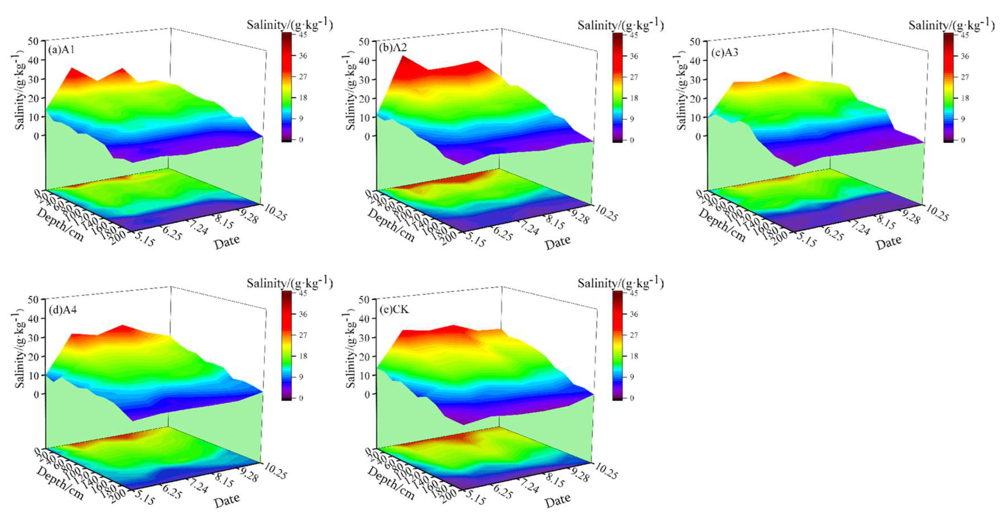
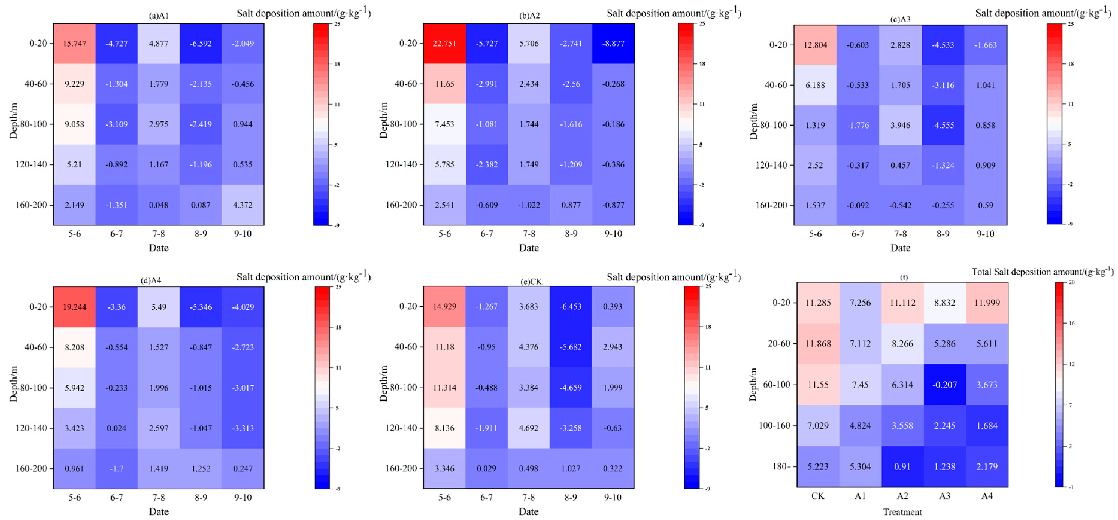
3.1. Change in the Salt Content of the Soil Profile During the Fertility Period

The change in salt content of the soil profile treated during the growth period from 15 May to 28 October 2024 is shown in Figure 2. According to Figure 2, in the spatial distribution, the salt content of the soil profile in each treatment showed a trend of high surface layer and low deep layer, and the salt content of the 0–20 cm soil layer was significantly higher than that of the deep soil. The average salt content ranged from 18.59 to 32.94 g·kg⁻¹, while the average salt content of the >20–200 cm soil layer ranged from 6.79 to 17.69 g·kg⁻¹. Further analysis showed that the soil salinity of the dark tube treatment increased with the dark tube spacing and decreased with the buried depth, which was higher than that of the no dark tube treatment. All treatments showed significant salt surface clustering except in October. In October, a significant reduction in surface soil salinity was observed across all treatments, primarily attributed to the implementation of the 70 cm deep tillage in the experimental plots. This tillage practice disrupted surface crust formation, enhanced precipitation infiltration, and facilitated salt redistribution through the mixing of high-salinity surface soil with low-salinity subsoil.

Soil salinity exhibits significant seasonal fluctuations. After leaching in May, soil salinity drops to its lowest point of the year. From June to October, as temperatures rise and evaporation intensifies, the soil enters a salt accumulation phase. Time series analysis shows that under identical treatment conditions, the 0–200 cm soil layer exhibits “bimodal” fluctuations: peak salt occurs in June and August (for A3 treatment, reaching 14.31 g·kg⁻¹ and 15.12 g·kg⁻¹, respectively), while in July and September to October, due to environmental factors, the salinity decreases (for A3 treatment, dropping to 13.81, 12.57, and 12.91 g·kg⁻¹, respectively). The June salinity peak was driven by rising temperatures, low surface vegetation coverage, and soil evaporation dominance, leading to upward salt migration and subsequent accumulation. In July, salinity decreased due to dense crop canopy coverage, enhanced transpiration that depleted soil moisture, and salt leaching from monsoon precipitation. A secondary salt accumulation phase occurred in August, triggered by leaf senescence, resurgent evaporation rates, and diminished salt leaching caused by reduced precipitation. The installation of subsurface pipes inhibits salt accumulation. The order of soil salinity ranges for each treatment is A3 (12.56–15.12 g·kg⁻¹) < A1 (13.90–16.46 g·kg⁻¹) < A2 (14.33–18.33 g·kg⁻¹) < A4 (14.50–18.55 g·kg⁻¹) < CK (16.50–20.31 g·kg⁻¹); CK treatment (no subsurface pipes) has a mean salinity 31.4% higher than the optimal treatment A3. Subsurface drainage engineering disrupts this positive feedback loop through dual mechanisms. Water Table Depression Effect: The drainage system effectively lowers the groundwater table, increasing capillary rise resistance and reducing upward water flux to surface layers. Leaching-Dilution Effect: Reduced spacing between subsurface drainage pipes enhances drainage capacity, accelerating lateral transport of soluble salts during irrigation or precipitation events.

3.2. Coupling Relationship Between Groundwater Depth and Soil Salinity

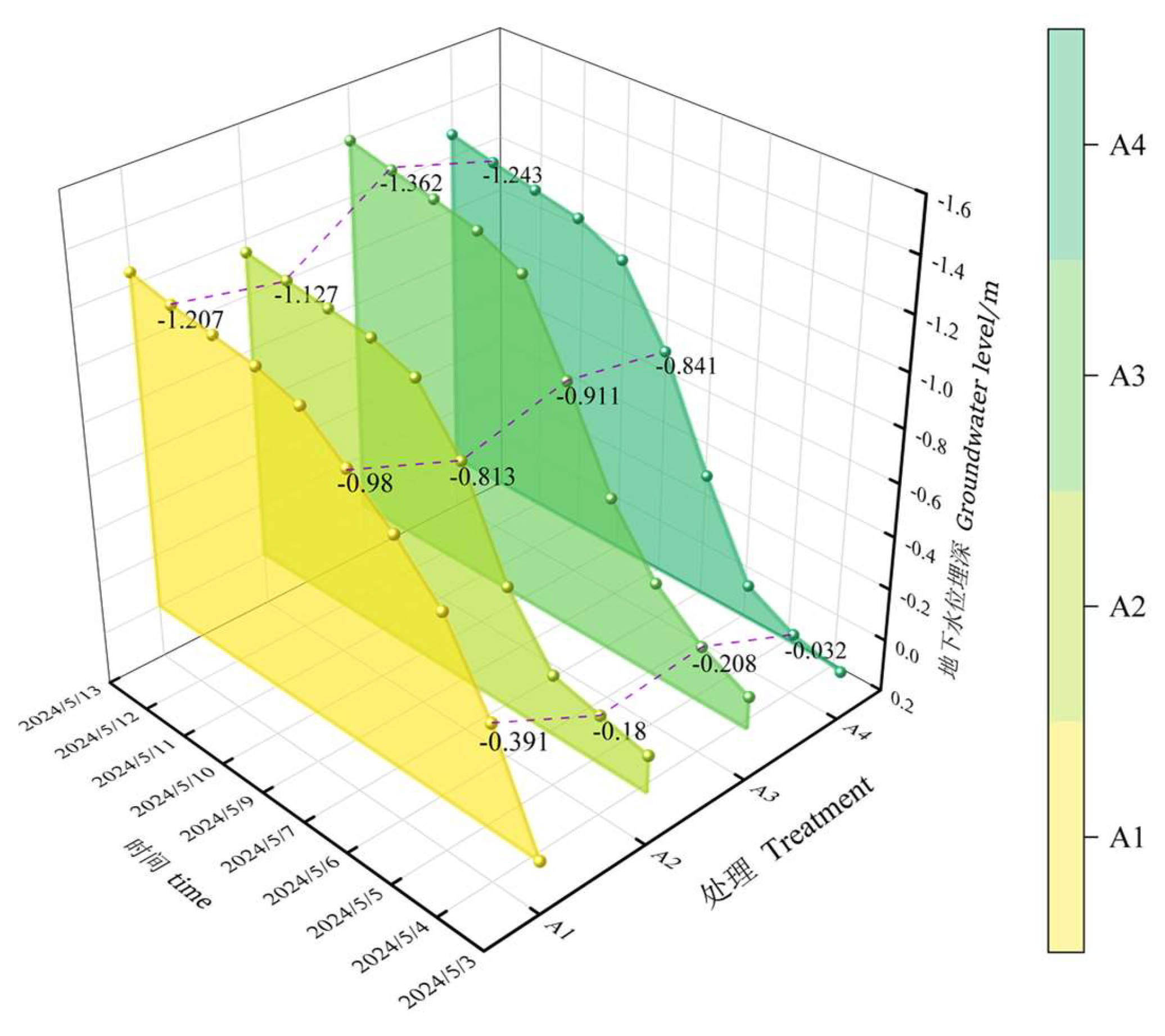
3.2.1. The Effect of the Dark Pipe on the Reduction of the Groundwater Burial Depth

This study investigates the variation patterns of groundwater level reduction under different concealed pipe layout methods after spring irrigation, with the initial condition being no surface water accumulation (or only a small amount of water) on the ground. The results are shown in Figure 3. Under the same concealed pipe spacing conditions, the treatment with a smaller burial depth (1.2 m) experienced faster groundwater level decline compared to the treatment with a larger burial depth (1.5 m) in the short term. As time extended, the treatment with a larger burial depth (1.5 m) showed a significantly accelerated rate of groundwater level decline. The primary reason for this phenomenon is that in the treatment with a smaller burial depth (1.2 m), the vertical distance between the groundwater level and the concealed pipes is shorter, resulting in a higher initial hydraulic gradient according to Darcy’s law, leading to a higher initial drainage rate and faster groundwater level decline. In contrast, the treatment with a larger burial depth (1.5 m) has a longer vertical distance, resulting in a slower initial drainage rate, but its conductivity is significantly improved, and the drainage influence radius is larger, thus demonstrating better groundwater level regulation effects over a longer time scale. Further comparative analysis shows that the groundwater burial depth reduction rates for treatments A1 to A4 within the same time frame were 12.42%, 10.12%, 12.77%, and 12.68%, respectively, ranking as A3 > A4 > A1 > A2. According to the two-factor ANOVA in

Table 3. Results of multi-factor ANOVA.

	Error Sum of Square	df	Square	F	p	Partial η2
Spacing	0.001	1	0.001	30.278	0.001 **	0.791
Depth	0.001	1	0.001	38.123	0.000 **	0.827
Spacing × Depth	0.000	1	0.000	2.358	0.163	0.228
Residual	0.000	8	0.000

Note: R² = 0.898, ** p < 0.01.

, the spacing main effect was significant (F = 30.278, p = 0.001, partial η² = 0.791), indicating that different spacings have a significant impact on the rate of groundwater reduction. The burial depth main effect was also significant (F = 38.123, p = 0.000, partial η² = 0.827), indicating that different burial depths significantly affect the rate of groundwater decline; through post-hoc comparisons in

Table 4. Results of post-hoc multiple comparisons for spacing and burial depth.

	MD	SE	t	p	Cohen’s d
20–40	0.017	0.003	5.503	0.001	3.177
1.2–1.5	−0.019	0.003	−6.174	0.000	−3.565

, it was found that as the spacing between pipes increases, the rate of groundwater burial depth decrease gradually decreases; however, with an increase in pipe burial depth, the rate of groundwater decline significantly increases. Since the burial depth is η² > spacing η², the impact of pipe burial depth on the rate of groundwater decline is more pronounced than that of spacing.

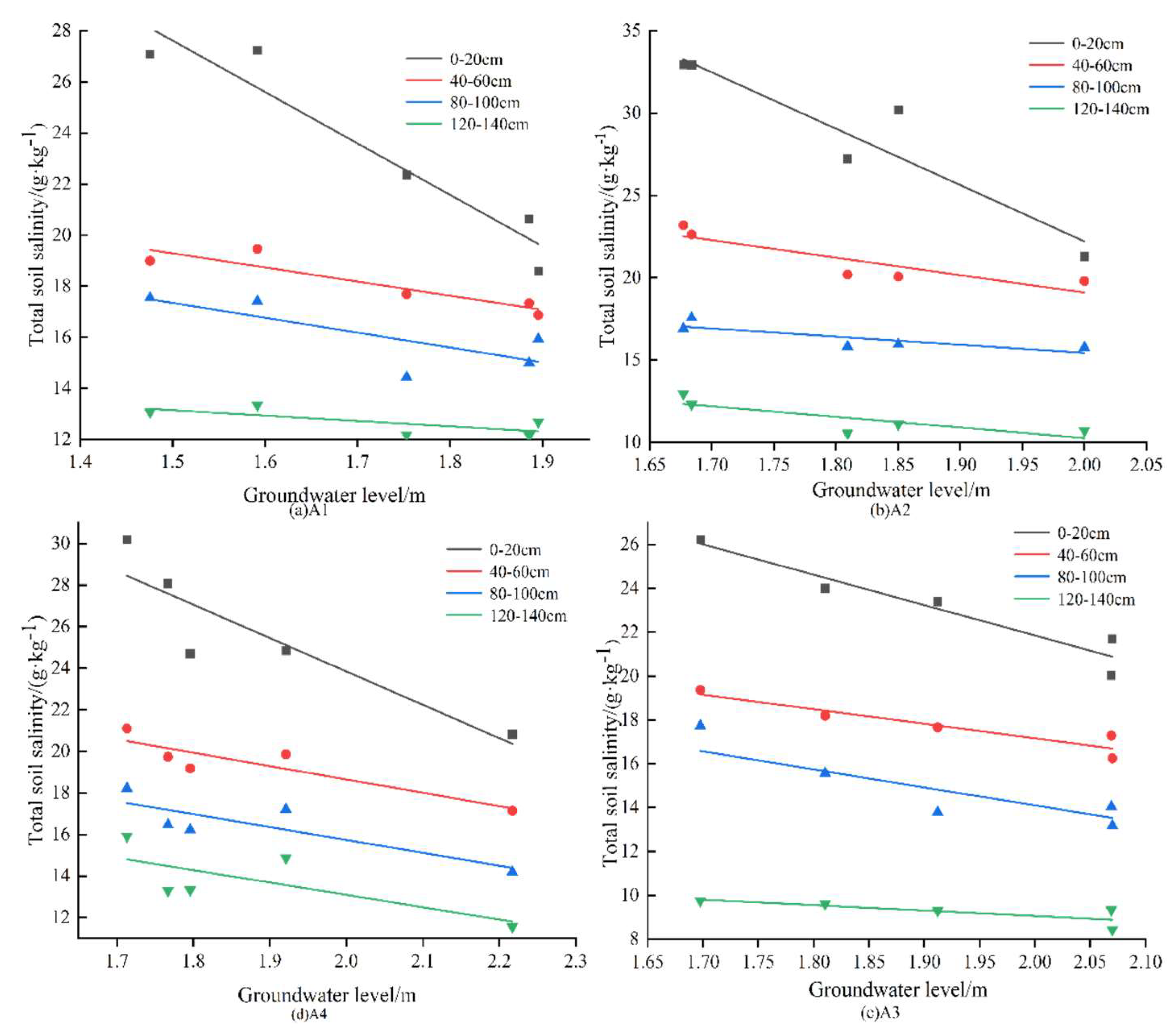
3.2.2. The Relationship Between Groundwater Buried Depth and Soil Salt

As can be seen from Figure 4, the total salt amount of different soil layers and the groundwater depth are significantly negatively correlated. This phenomenon fundamentally reflects the depth-dependent nature of capillary-driven salt transport. When the groundwater table depth is below the critical height (*h*), capillary action sustains continuous upward migration of saline water to the soil surface. Based on the test data in Figure 4, the equations were fitted to each soil layer, and the specific results are shown in

Table 5. Different soil layers are shown as coupling equations between soil salinity and groundwater depth.

Depth/cm	Fitting Equation				R2
	A1	A2	A3	A4	A1	A2	A3	A4
0–20	y = −20.1284x + 57.80725	y = −34.24075x + 90.68594	y = −13.84332x + 49.54053	y = −16.04791x + 55.93775	0.917	0.881	0.919	0.817
40–60	y = −5.52997x + 27.58208	y = −10.6204x + 40.33789	y = −6.61504x + 30.39591	y = −6.42782x + 31.50319	0.841	0.784	0.878	0.802
80–100	y = −5.81952x + 26.07549	y = −4.95533x + 25.34552	y = −10.22076x + 34.4067	y = −6.19247x + 28.11942	0.586	0.684	0.825	0.704
120–140	y = −2.09952x + 16.29413	y = −6.43368x + 23.13112	y = −2.46006x + 13.98265	y = −5.942x + 24.97841	0.529	0.671	0.604	0.516

Note: y denotes total soil salt content, and x represents groundwater table depth.

. Among them, the correlation coefficient (R²) shows a trend of 0–20 cm > 40–60 cm > 80–100 cm > 120–140 cm, and the slope of the equation increases with the increase of soil depth. This shows that the change of groundwater depth has the most significant effect on the salinity of the 0–20 cm soil layer, while the effect on the 40–60 cm, 80–100 cm, and 120–140 cm soil layers is weakened. The primary mechanism lies in the depth-dependent capillary dynamics. At shallow groundwater table depths, the capillary water flux density increases significantly, driving salt enrichment in surface layers through evaporative concentration. However, as soil depth increases, the influence of groundwater table depth on salinity diminishes due to attenuated capillary action and altered soil pore structure. Moreover, the correlation coefficient of the 180 to 200 cm soil layer is R² < 0.5, so it is not fitted to equations. Regulating the buried depth of groundwater through the dark pipe can effectively reduce the soil salt and alleviate the soil salinization problem caused by strong evaporation.

3.3. Salt Content Change in Soil Section Area During the Fertility Period

The salt accumulation of each treated soil during the growth period is shown in Figure 5. Spatially, salt accumulation exhibited a decreasing trend with increasing soil depth. The surface salt accumulation of 0–20 cm is 10.097 g·kg⁻¹, and the salt accumulation below >160 cm is 2.971 g·kg⁻¹. In terms of time, the soil accumulated salt from May to June and from July to August, while the rest of the months showed a desalination state. From May to June, the soil salt accumulation was the largest, and the salt accumulation of the CK treatment was relatively low. The main reason was that the sample was taken after irrigation on 15 May, and the soil salt content was low. Therefore, the salt accumulation in each treatment from May to June was the most significant, while for CK, the effect of irrigation on soil desalination was limited. In this study, the variation of salt accumulation of each soil layer from May to October was taken as the total salt accumulation. Taking the 0–60 cm soil layer as an example, the total salt accumulation of CK treatment was 23.153 g·kg⁻¹, while A1, A2, A3, and A4 treatment reduced 8.785 g·kg⁻¹, 3.775 g·kg⁻¹, 9.035 g·kg⁻¹, and 5.543 g·kg⁻¹ compared with CK treatment, respectively. That is, at the same spacing of the dark pipe, the total salt accumulation increases with the increase of the same spacing. Overall, the total soil salt accumulation was A3 (1.5 m, 20 m) among the five treatments.

According to

Table 6. Results of multi-factor ANOVA.

	Error Sum of Square	df	Square	F	p	Partial η2
Spacing	33.260	1	33.260	9.107	0.017 *	0.532
Depth	40.407	1	40.407	11.064	0.010 *	0.580
Spacing × Depth	5.661	1	5.661	1.550	0.248	0.162
Residual	29.216	8	3.652

Note: R² = 0.679, * p < 0.05.

, further analysis in

Table 7. Results of post-hoc multiple comparisons for spacing and burial depth.

	MD	SE	t	p	Cohen’s d
20–40	−3.330	1.103	−3.018	0.017	−1.742
1.2–1.5	3.670	1.103	3.326	0.010	1.920

shows that the main spacing effect is significant (F = 9.107, p = 0.017), indicating a significant difference in soil salinization effects at different spacings. Post-hoc multiple comparisons revealed that when the spacing was 20.0–40.0 m, the mean difference in salt accumulation was −3.330 (p < 0.05), suggesting that a smaller spacing (20.0) significantly reduces soil salinization. The depth main effect is also significant (F = 11.064, p = 0.010), indicating a significant impact of different depths on salt accumulation. Post-hoc multiple comparisons showed that when the depth was 1.2–1.5 m, the mean difference in salt accumulation was 3.670 (p < 0.05), indicating that a larger depth (1.5 m) significantly reduces soil salinization. Therefore, a spacing of 20 m and a depth of 1.5 m in this region can more effectively suppress salinity.

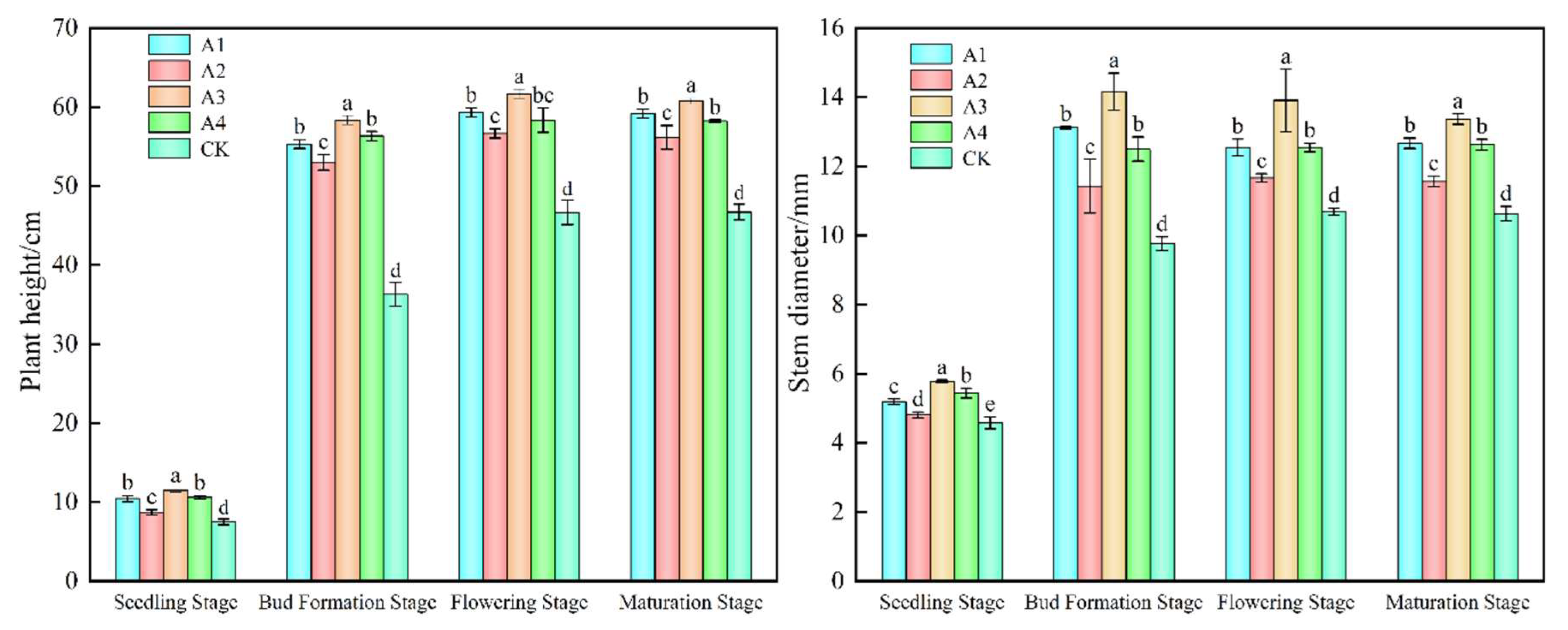
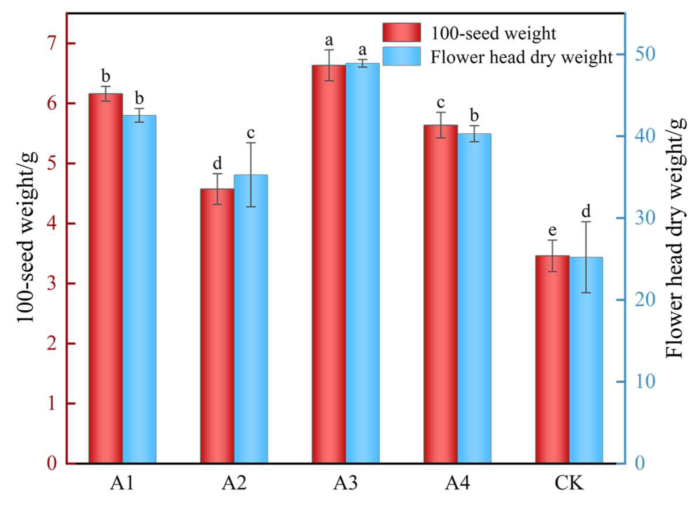
3.4. Effects of Different Treatments on Growth Indexes of Sunflowers

The 2024 full-observation study demonstrated significant regulatory effects of subsurface drainage treatments (A1–A4) on sunflower agronomic traits (see Figure 6). Systematic measurements of plant height, stem diameter, capitulum dry weight, and 100-seed dry weight revealed three-phase growth dynamics (“rapid–slow–stagnant”) across all treatments. Plant height peaked from the bud stage to the flowering stage, followed by a slight decline during maturation due to reproductive growth prioritization. Treatment A3 (1.5 m burial depth, 20 m spacing) exhibited optimal performance, with plant height (39.9–93.9% increase vs. CK) and stem diameter (32.18–91.71% increase at bud stage) showing significant superiority over other treatments (p < 0.05) and highly significant differences from CK (p < 0.01). Under saline soil conditions, capitulum dry weight and 100-seed dry weight were adopted as alternative evaluation metrics (see Figure 7). Treatment A3 achieved values of 49.86 g and 6.63 g, respectively, representing 93.9% and 91.7% increases over CK (25.21 g, 3.46 g). These improvements significantly exceeded those of A1 (68.7%), A4 (59.8%), and A2 (39.9%) treatments (p < 0.05). This phenomenon fundamentally reflects the extent of salt-induced inhibition alleviation on crop physiological processes. Subsurface drainage treatments, particularly A3, effectively mitigated salt stress by reducing root zone salinity. The study confirms that an optimized subsurface drainage configuration (1.5 m × 20 m) enhances sunflower morphogenesis and reproductive development through root zone environment amelioration, providing theoretical guidance for saline farmland management.

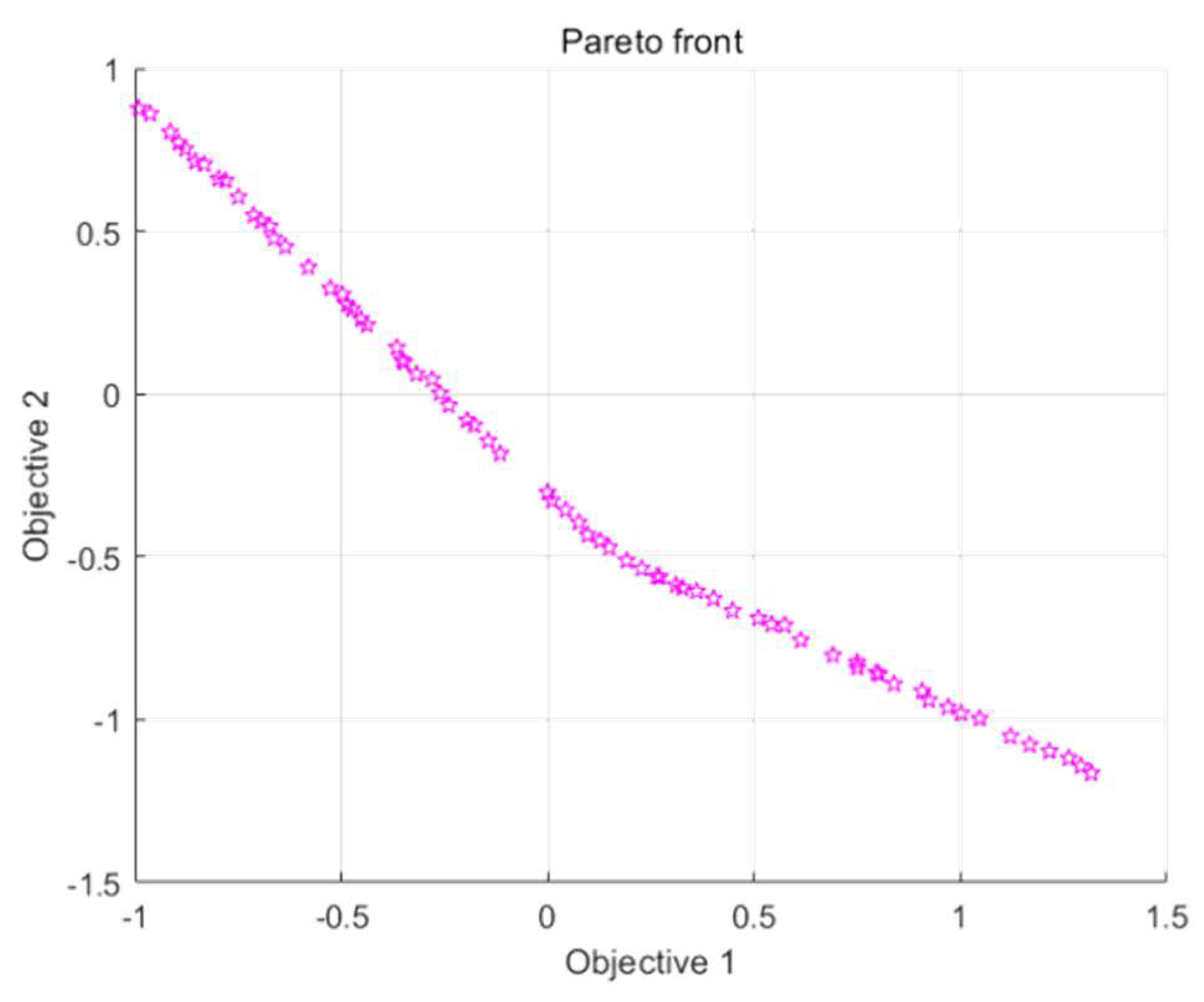
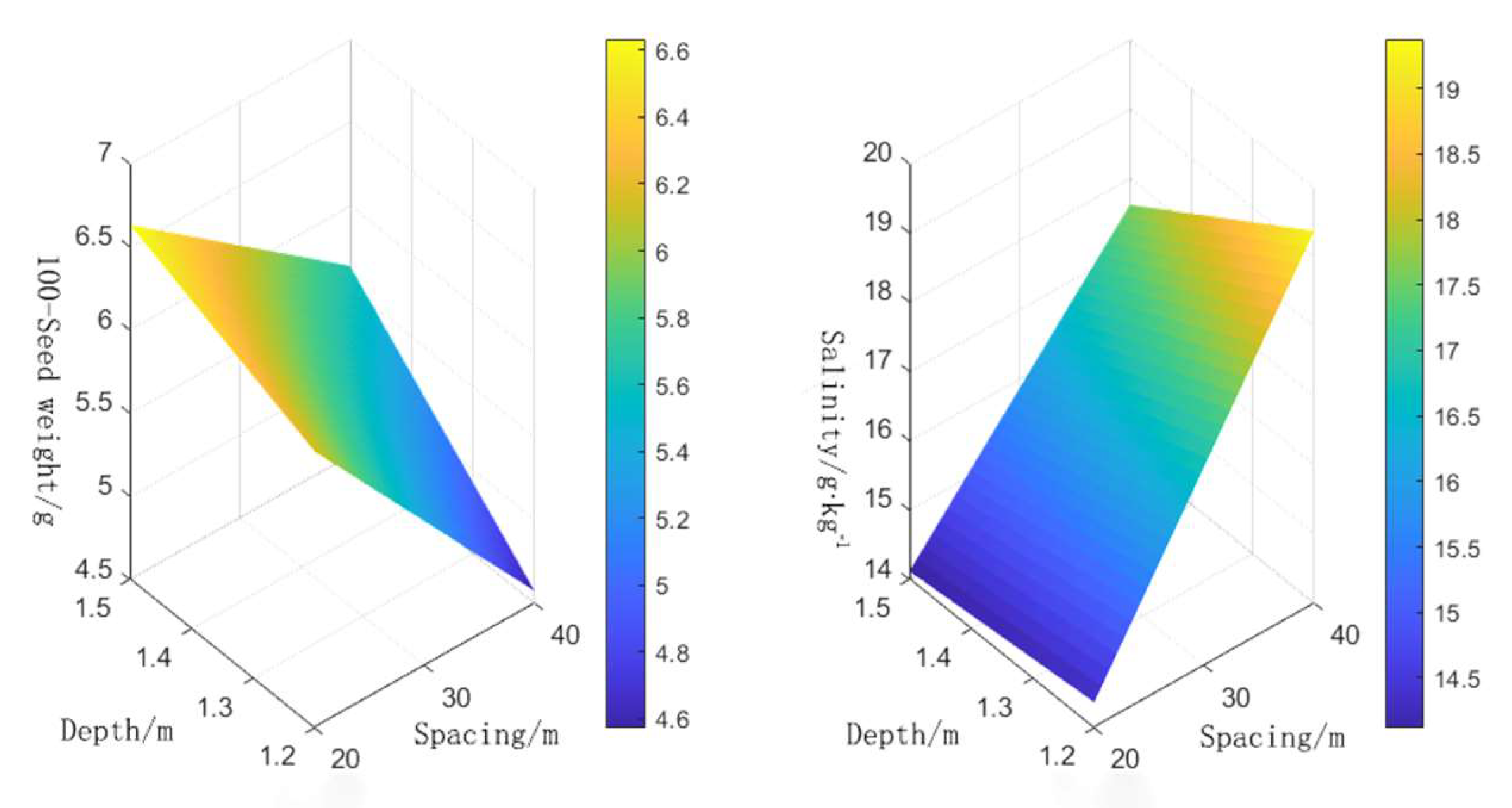
3.5. The Parameters of Dark Pipe Layout Are Optimized by Multi-Objective Genetic Algorithm

Due to the spacing of field experiments (20, 40), there are four combinations of buried depth (1.2, 1.5), but there is a lack of research on whether there is a better spacing and buried depth. Therefore, adopt the multi-target genetic algorithm, consider engineering benefits and economic benefits, take the dry 100-seed weight as target 1, and select 0–60 cm salt accumulation as target 2 to optimize the buried depth and spacing. Parameter configuration: population size 100, maximum number of iterations 200, Pareto solution ratio 0.7, crossover probability 0.8, convergence threshold 1 × 10⁻⁴. Build the interpolation function of the target and form the Pareto front map (see Figure 8).

Based on the existing spacing and depth, the Pareto optimization solution and the output of dry seed weight per hundred seeds, as well as root zone salinity, were obtained through a multi-objective genetic algorithm, as shown in

Table 8. Pareto optimized solutions.

Spacing (m)	Depth (m)	100-Seed Weight (g)	Root Zone Salinity (g·kg−1)	Spacing (m)	Depth (m)	100-Seed Weight (g)	Root Zone Salinity (g·kg−1)
25.158	1.4856	6.3461	15.049	23.094	1.48	6.4413	14.691
20.028	1.4969	6.6267	14.125	39.692	1.4372	5.4316	17.921
39.947	1.2025	4.5861	19.35	39.752	1.2236	4.676	19.178
24.98	1.4901	6.3646	15.008	37.811	1.4899	5.7125	17.281
38.352	1.4897	5.6843	17.379	39.822	1.3761	5.2086	18.304
34.108	1.4925	5.908	16.614	30.539	1.487	6.0741	16.004
39.603	1.3982	5.2996	18.131	39.555	1.2972	4.9488	18.705
39.626	1.2091	4.6345	19.232	39.628	1.3906	5.2716	18.179
23.094	1.4878	6.456	14.678	20.21	1.4874	6.6025	14.166
32.696	1.4932	5.9815	16.362	39.948	1.4197	5.3553	18.073
39.936	1.2513	4.7597	19.061	39.937	1.4497	5.462	17.895
35.503	1.4972	5.8523	16.838	37.001	1.4892	5.7512	17.142
33.357	1.4982	5.9627	16.458	39.659	1.2642	4.8257	18.92
29.694	1.4953	6.1383	15.826	39.752	1.4809	5.582	17.678
39.873	1.3576	5.1399	18.423	39.867	1.4624	5.5108	17.807
39.913	1.2392	4.7185	19.126	39.795	1.2056	4.6089	19.294
39.952	1.3219	5.0087	18.649	24.758	1.4926	6.3809	14.964
39.954	1.3442	5.0873	18.519	34.872	1.4952	5.8778	16.737
39.071	1.4947	5.665	17.478	28.751	1.4932	6.1807	15.667
28.019	1.4928	6.2167	15.539	33.946	1.4949	5.9236	16.575
23.883	1.4868	6.4138	14.82	26.179	1.4943	6.3129	15.21
28.936	1.4926	6.1698	15.701	21.017	1.4864	6.5595	14.31
39.888	1.2802	4.8653	18.88	31.43	1.4981	6.0586	16.121
39.855	1.4732	5.5496	17.742	21.792	1.4908	6.5276	14.443
29.436	1.4952	6.151	15.781	39.111	1.4878	5.6389	17.524
37.505	1.494	5.7416	17.206	39.336	1.4854	5.6192	17.578
22.396	1.4956	6.5058	14.543	27.065	1.4922	6.2635	15.372
39.943	1.4538	5.4761	17.872	22.434	1.4862	6.4868	14.563
39.239	1.3757	5.2435	18.186	31.319	1.4976	6.0628	16.103
28.155	1.4849	6.1909	15.586	39.752	1.3273	5.041	18.574
21.529	1.4911	6.5414	14.396	31.898	1.4849	5.999	16.253
39.882	1.2881	4.8936	18.832	25.853	1.498	6.3371	15.145
39.71	1.3281	5.0467	18.56	39.571	1.3372	5.0878	18.477
39.937	1.4653	5.5173	17.803	31.947	1.498	6.0324	16.212
39.657	1.4264	5.3956	17.977	39.976	1.3014	4.9342	18.775

. The optimized solution shows that dry grain weight per hundred grains (6.0~6.6 g) is negatively correlated with salt accumulation (14~19 g·kg⁻¹), which aligns with the characteristics of multi-objective trade-offs. For the optimal solution distribution, high dry grain weight per hundred grains (>6.4 g): spacing 20~25 m, depth 1.48~1.5 m, salinity 14~15 g·kg⁻¹; low salt accumulation (<15 g·kg⁻¹): some yield must be sacrificed (dry grain weight per hundred grains approximately 6.3~6.6 g); extreme parameters (spacing ≈ 40 m, depth ≈ 1.2 m) result in high salinity (19 g·kg⁻¹) and low yield (<5 g), which should be avoided. For the parameter space distribution pattern, see Figure 9. Spacing: smaller spacing (20~30 m) is more conducive to high yield and reduces salt accumulation; larger spacing (>35 m) increases salt accumulation and decreases yield. Depth: deep burial (1.45~1.5 m) helps control salinity and increase yield; shallow burial (1.2~1.4 m) has the opposite effect.

The entropy weight method was applied to assign weights to the 100-seed weight and root zone salinity indicators from the Pareto-optimal solutions. A comprehensive evaluation was then conducted using the TOPSIS (Technique for Order Preference by Similarity to Ideal Solution) method to identify the optimal subsurface drainage pipe configuration, presented in

Table 9. Summary of entropy weight method calculation results.

	e	d	Weight Coefficient w
root zone salinity	0.9950	0.0050	53.7869%
100-seed weight	0.9957	0.0043	46.2131%

and

Table 10. Results of TOPSIS model evaluation.

Spacing (m)	Depth (m)	Relative Proximity C	Sorting Results	Spacing (m)	Depth (m)	Relative Proximity C	Sorting Results
20.028	1.4969	1	1	37.811	1.4899	0.475	36
20.21	1.4874	0.99	2	38.352	1.4897	0.459	37
21.017	1.4864	0.966	3	39.071	1.4947	0.445	38
21.529	1.4911	0.953	4	39.111	1.4878	0.435	39
21.792	1.4908	0.945	5	39.336	1.4854	0.425	40
22.396	1.4956	0.93	6	39.752	1.4809	0.407	41
22.434	1.4862	0.923	7	39.855	1.4732	0.393	42
23.094	1.4878	0.905	8	39.937	1.4653	0.379	43
23.094	1.48	0.9	9	39.867	1.4624	0.377	44
23.883	1.4868	0.881	10	39.943	1.4538	0.363	45
24.758	1.4926	0.858	11	39.937	1.4497	0.357	46
24.98	1.4901	0.85	12	39.692	1.4372	0.347	47
25.158	1.4856	0.842	13	39.657	1.4264	0.333	48
25.853	1.498	0.83	14	39.948	1.4197	0.314	49
26.179	1.4943	0.818	15	39.603	1.3982	0.295	50
27.065	1.4922	0.79	16	39.628	1.3906	0.283	51
28.019	1.4928	0.762	17	39.239	1.3757	0.275	52
28.155	1.4849	0.752	18	39.822	1.3761	0.256	53
28.751	1.4932	0.741	19	39.873	1.3576	0.228	54
28.936	1.4926	0.735	20	39.571	1.3372	0.209	55
29.436	1.4952	0.723	21	39.954	1.3442	0.206	56
29.694	1.4953	0.716	22	39.71	1.3281	0.191	57
30.539	1.487	0.683	23	39.752	1.3273	0.189	58
31.319	1.4976	0.671	24	39.952	1.3219	0.174	59
31.43	1.4981	0.668	25	39.555	1.2972	0.153	60
31.947	1.498	0.653	26	39.976	1.3014	0.143	61
31.898	1.4849	0.641	27	39.882	1.2881	0.127	62
32.696	1.4932	0.626	28	39.888	1.2802	0.115	63
33.357	1.4982	0.612	29	39.659	1.2642	0.101	64
33.946	1.4949	0.592	30	39.936	1.2513	0.072	65
34.108	1.4925	0.584	31	39.913	1.2392	0.055	66
34.872	1.4952	0.565	32	39.752	1.2236	0.039	67
35.503	1.4972	0.55	33	39.626	1.2091	0.023	68
37.001	1.4892	0.497	34	39.795	1.2056	0.011	69
37.505	1.494	0.489	35	39.947	1.2025	0	70

. The results show that the spacing is 20.028 m, and the buried depth of 1.4969 m is the maximum progress C, which is consistent with the optimal spacing of 20 m and the buried depth of 1.5 m. Based on the above results, it is suggested to adopt the buried depth of 1.5 m and spacing of 20 m in this area to realize the maximum benefit of soil salt regulation and crop growth.

4. Discussion

4.1. Effect of Dark Tube on Soil Salt Accumulation

This study has elucidated a tripartite coupling mechanism through which subsurface drainage systems suppress surface salt accumulation via groundwater table dynamics regulation: capillary-driven vertical salt migration, evaporation-potential-dominated surface salt enrichment, and drainage parameter-mediated groundwater level control. Vertical stratification analysis revealed significantly higher salt accumulation in the 0–20 cm surface layer (10.097 g·kg⁻¹) compared to subsoil (>160 cm depth: 2.971 g·kg⁻¹), quantitatively validating capillary rise-dominated salt surface aggregation processes (Figure 5). The drainage system disrupts the “evaporation–accumulation” positive feedback loop by depressing groundwater tables, thereby reducing capillary water fluxes. Among them, the average total salt accumulation of 0~60 cm soil layer with A3 treatment (20 m spacing and buried depth of 1.5 m) decreased by 9.035 g·kg⁻¹ compared with CK, indicating that the dark pipe effectively blocked the migration of the salt layer to the surface by optimizing the dynamic regulation of the groundwater level. This result is consistent with the study of Wang [24], which pointed out that the drainage reduces the rising effect of capillary tubes by inhibiting the accumulation of salt in the cultivation layer. Temporal dynamics revealed a distinct salt accumulation peak during May–June, with the control group (CK) showing significantly lower accumulation. This pattern originated from post-irrigation (15 May) differential responses: subsurface drainage treatments rapidly evacuated saline percolation water, whereas CK developed a “irrigation–stagnation–accumulation” vicious cycle due to lacking drainage pathways, leading to surface salt re-accumulation via evaporative pumping. ANOVA demonstrated significant main effects of both drainage spacing (F = 9.107, p = 0.017) and burial depth (F = 11.064, p = 0.010); the increase of spacing (such as A2 and A4) leads to the decrease of drainage efficiency, the increase of salt retention in local areas, and the increase of buried depth (such as A3) accelerates the decline rate of the groundwater level and further strengthens the desalination effect (Table 6). The observed lower salt accumulation in the A3 system compared to shallow systems (A1/A2) aligns with enhanced hydraulic connectivity between drainage pipes and the active root zone (0–60 cm). However, in the A4 configuration (1.5 m depth × 40 m spacing), a spacing-depth trade-off emerges, as the excessively wide spacing increases groundwater table rebound frequency, thereby offsetting the benefits of deeper installation. This is consistent with the results of Long [25], which state that increasing the depth of the buried pipe can expand the influence range of drainage and shorten the salt migration path. The results showed that the drainage was significantly effective in reducing soil salinity, inhibiting secondary salinization, and increasing crop yield [26]. This study recommends subsurface drainage systems with optimal parameters (1.5 m burial depth × 20 m spacing) combined with synchronized irrigation leaching as an integrated strategy for arid/semi-arid regions, demonstrating dual effectiveness.

4.2. The Influence of Groundwater Burial Depth on Soil Salinity

This study shows that there is a significant negative correlation between groundwater depth and soil salinity (R² = 0.529–0.919) (Table 5). Specifically, in 0–20 cm surface soil, the salt content increased by 13.84–34.24 g·kg⁻¹ (fitting equation according to different treatments). This is consistent with the results of Liu [27] on the negative correlation between diving depth and salt accumulation. This phenomenon originates from the tripartite coupling mechanism of “evaporation–capillarity–salt migration”, unique to arid regions. Elevated groundwater tables accelerate capillary front advancement to the soil surface, thereby increasing daily salt flux density through preferential flow paths. These hydrogeochemical dynamics drive rapid surface salt accumulation via dominant vertical transport pathways [28]. The July/September rainfall-induced salt redistribution reveals a hydrological memory effect; despite temporary groundwater rise, subsurface drainage accelerated post-precipitation water table recession by 40% versus CK, curtailing salt re-accumulation. This demonstrates drainage’s dual functionality. For deep soil (under 160 cm), the response to groundwater depth change was weak (R² < 0.5). In addition, the dark pipe treatment controlled the groundwater level below 1.6 m by active drainage, which significantly reduced the evaporation-driven salt surface concentration effect. This method is highly consistent with the critical buried depth theory proposed by Xu [29] based on the instruction Kriging method (i.e., inhibiting salt surface aggregation by controlling the groundwater level below the capillary rise limit depth). Field experiments revealed that in arid/semi-arid regions with high groundwater mineralization, conventional 1.5 m drainage depth proves insufficient to intercept capillary-driven salt resurgence pathways due to intensive evaporative demand. We therefore recommend increased burial depths for these areas. Conversely, in zones with lower mineralization, shallower configurations achieve effective salt control with cost reduction. To sum up, in the salinization treatment in arid areas, dynamic monitoring of groundwater level and precise control combined with dark tube technology are the key strategies to inhibit salt surface aggregation.

4.3. The Influence of Dark Pipe Layout on the Change of Crop Growth Index

The growth index, dry matter accumulation, and 100-seed weight all showed high levels, and the differences among the treatments were significant (p < 0.05). In this study, we compared the effect of dark tube treatment with that of no dark tube treatment, and the results show that the growth indexes of dark tube treatment are significantly better than that of no dark tube treatment, which is consistent with the conclusion of the Jiao [30] study that the growth index of crops in dark tube areas is better than that of no dark tube treatment. The layout of the dark tube significantly improved the growth environment of oil sunflowers, and the A3 treatment was particularly prominent, and the plant height (93.9% higher than CK), stem diameter, disk dry weight (93.9% higher), and 100-seed weight (91.7% higher) all reached the optimal level. This result is closely related to the physiological response mechanism of crops under salinity stress. Saline accumulation will inhibit water and nutrient uptake by crop roots, disrupt cell membrane stability, and reduce photosynthetic efficiency [31]. A3 treatment controlled 0–20 cm of soil salt at 11.60–22.80 g·kg⁻¹ (significantly lower than 12.15–28.13 g·kg⁻¹ of CK), which effectively alleviated the salt stress and promoted the root development and the accumulation of photosynthates. The vertical salt displacement achieved through subsurface drainage likely disrupted the toxic ion accumulation zone near root hairs; this mechanistic explanation resolves previous uncertainties about minimum salt displacement distances for sunflower cultivars.

Moreover, dark pipe drainage may enhance the stress resistance of crops [32] by improving soil aeration and enhancing oxygen supply in the root area, but long-term sustainability requires evaluation of salt redistribution patterns beyond single growing seasons.

4.4. Subsurface Drainage Parameter Optimization

This study employed a multi-objective genetic algorithm combined with entropy-weighted TOPSIS to optimize subsurface drainage parameters, targeting 100-seed dry weight maximization and salt accumulation minimization. Using natural neighbor interpolation functions calibrated to experimental data within predefined ranges, the results demonstrated that smaller spacings and greater depths yielded Pareto-optimal solutions that align with the fundamental principles of subsurface hydrology; increased depth enhances capillary barrier disruption, reducing upward salt flux during evaporation, while narrower spacing improves lateral drainage efficiency, accelerating salt leaching during irrigation events. These findings align with Guo’s [33] conclusion recommending 1.5 m depth × 20 m spacing derived via entropy TOPSIS.

Limitations include (1) parameter constraints restricting extrapolation beyond tested ranges, extrapolation to extreme conditions requires caution. Shallow water tables common in arid regions may alter flux dynamics, necessitating site-specific adjustments to the generalized interpolation functions. (2) Algorithmic sensitivity to hyperparameters requiring empirical calibration, and (3) lack of explicit physical mechanisms governing soil–water–salt dynamics. Liu [34] and Ding [35] demonstrated that the HYDRUS-2D model exhibits high reliability in optimizing subsurface drainage parameters and simulating salt accumulation/leaching processes. As a physics-based tool, HYDRUS-2D has become central to soil water–salt studies due to its mechanistic analysis, multi-scenario validation, and decision support capabilities. However, its application in single-objective frameworks limits its ability to address complex trade-offs; future work will integrate process-based models (HYDRUS-2D/SWAP) to simulate water–salt transport under diverse drainage configurations, followed by MOGA optimization to balance desalination efficiency, salt suppression, and yield enhancement.

This study revealed that subsurface drainage systems effectively suppress surface salt accumulation and enhance crop growth indicators through groundwater table dynamics regulation, with optimal performance achieved under the 1.5 m burial depth × 20 m spacing configuration. Simplified Drivers: The analysis focused on spacing, depth, and groundwater table impacts, neglecting synergistic effects of climatic variability (e.g., extreme drought/rainfall cycles); soil textural heterogeneity (tested only on silt loam); groundwater mineralization gradients; and crop water stress dynamics under arid conditions. However, since this study primarily focuses on the impact of spacing, burial depth, and groundwater depth on soil salinization, the salinization process is also influenced by multiple factors such as climate, soil texture, and groundwater mineralization. For crops, this paper only considers salt content and does not take into account the water effects under drought conditions. Moreover, regarding how to handle pollutants discharged from subsurface pipes that damage the ecological environment, it fails to consider the cost–benefit comparison of subsurface pipes, as well as the water resource shortages in semi-arid and arid regions. It also does not consider the optimal drainage quota parameters for subsurface pipe layout and conducts only one-year trials; thus, traditional physical model simulations have not been performed. Future research needs to comprehensively consider these factors, further expand the trials to verify their applicability, and optimize solutions.

5. Conclusions

The average total accumulated salt amount in A3 (spacing 20 m, depth 1.5 m) was the lowest (May to October), which was 9.035 g·kg⁻¹ less than that in the CK treatment.

The groundwater burial depth is negatively correlated with the soil salinity, and the groundwater burial depth has the greatest influence on the soil salinity in the topsoil of 0–20 cm; the burial depth is more important than the spacing for reducing the groundwater burial depth.

The plant height, stem diameter, dry 100-seed weight, and dry weight of the flower head of the sunflower were A3 > A1 > A4 > A2 > CK. The growth indexes of dark pipe treatment were significantly higher than those of the CK treatment, and the A3 treatment was the best.

Based on the multi-objective genetic algorithm and TOPSIS model, the optimal layout of the dark pipe in Yanqi Basin, southern Xinjiang, is 20 m spacing and 1.5 m depth. This provides regional policymakers and irrigation managers with a practical tool to develop salt control and irrigation strategies, effectively reducing soil salinity while supporting sustainable crop production in arid agricultural systems.

References

1. Wang, S.R.; Huang, Y.X. Research progress on saline-alkali land improvement in Songnen Plain. Soil Crop. 2023, 12, 206–217. [Google Scholar] [CrossRef]
2. Guo, B.; Yang, F.; Fan, Y.W.; Han, B.M.; Chen, S.T.; Yang, W.N. Dynamic monitoring of soil salinization in Yellow River Delta utilizing MSAVI–SI feature space models with Landsat images. Environ. Earth Sci. 2019, 78, 308. [Google Scholar] [CrossRef]
3. Yang, J.S.; Yao, R.J.; Wang, X.P.; Xie, W.P.; Zhang, X.; Zhu, W.; Zhang, L.; Sun, R.J. Research on salt-affected soils in China: History, status quo and prospect. Acta Petrol. Sin. 2022, 59, 10–27. [Google Scholar] [CrossRef]
4. Chang, X.M.; Gao, Z.Y.; Wang, S.L.; Chen, H.R. Modelling long-term soil salinity dynamics using SaltMod in Hetao irrigation District, China. Comput. Electron. Agric. 2019, 156, 447–458. [Google Scholar] [CrossRef]
5. Sun, G.F.; Zhu, Y.; Ye, M.; Yang, J.Z.; Qu, Z.Y.; Mao, W.; Wu, J.W. Development and application of long-term root zone salt balance model for predicting soil salinity in arid shallow water table area. Agric. Water Manag. 2019, 213, 486–498. [Google Scholar] [CrossRef]
6. Wichelns, D.; Qadir, M. Achieving sustainable irrigation requires effective management of salts, soil salinity, and shallow groundwater. Agric. Water Manag. 2015, 157, 31–38. [Google Scholar] [CrossRef]
7. Okur, B.; Örçen, N. Soil salinization and climate change. In Climate Change and Soil Interactions; Elsevier: Amsterdam, The Netherlands, 2020; pp. 331–350. [Google Scholar] [CrossRef]
8. Liu, H.J.; Liu, H.J.; Tan, L.M.; Liu, J.-T. Simulating the changes of water table depth in coastal saline land with agro-subsurface drainage system. Chin. J. Eco-Agric. 2012, 20, 1687–1692. [Google Scholar] [CrossRef]
9. Liu, Y.G.; Yang, H.C.; Wang, K.Y.; Lu, T.; Zhang, F. Shallow subsurface pipe drainage in Xinjiang lowers soil salinity and improves cotton seed yield. Trans. Chin. Soc. Agric. Eng. 2014, 30, 84–90. [Google Scholar] [CrossRef]
10. Jafari-talukolaee, M.; Ritzema, H.; Darzi-naftchali, A. Subsurface drainage to enable the cultivation of winter crops in consolidated paddy fields in Northern Iran. Sustainability 2016, 8, 249. [Google Scholar] [CrossRef]
11. Zhang, L.; Jiao, P.J.; Dong, Q.G.; Tao, Y. Effects of spacing and depth of subsurface drain on water and salt transport in the field. J. Irrig. Drain. 2023, 42, 92–101. [Google Scholar] [CrossRef]
12. Zhu, Z.; Wang, H.J.; Su, T.; Shi, X.-Y.; Song, J.-H.; Zhu, Y.-Q.; Zheng, Q. Research on Salt Discharge Effect of Different Buried Deep Pipes in Salinized Farmland. Xinjiang Agric. Sci. 2018, 55, 1523–1533. [Google Scholar]
13. Yang, Y.H.; Zhou, X.G.; Li, D.W.; Ji, Q. The Efficacy of Subsurface Drain in Desalinizing Cotton Field with Shallow Groundwater and Mulched Drip-irrigation in Southern Xinjiang. J. Irrig. Drain. 2021, 40, 137–144. [Google Scholar] [CrossRef]
14. Shi, L.; Lv, N.; He, S.; Yin, F.H.; Gao, Z.J.; Tan, X.R. Screening of the water drainage and salt control mode of subsurface pipe and shaft on the secondary salinization soil and its effect evaluation. Xinjiang Agric. Sci. 2022, 59, 716–724. [Google Scholar] [CrossRef]
15. Wen, Y.; Wang, Z.H.; Chen, L. Effects of buried depth of subsurface pipe on water and salt transport and oil sunflower yield under drip irrigation. J. Shihezi Univ. 2021, 39, 183–189. [Google Scholar] [CrossRef]
16. Ebrahimian, H.; Noory, H. Modeling paddy field subsurface drainage using HYDRUS-2D. Paddy Water Environ. 2015, 13, 477–485. [Google Scholar] [CrossRef]
17. Qian, Y.Z.; Zhu, Y.; Huang, J.S.; Jingwei, W.; Chang, A.; Shuai, H. Key parameters for the optimal layout of subsurface drainage pipe in arid areas. Trans. Chin. Soc. Agric. Eng. 2021, 37, 117–126. [Google Scholar] [CrossRef]
18. Qi, Q. Response of sunflower growth and water nitrogen transport to different nitrogen fertilizers and field drainage simulation under dark pipe drainage. Inner Mong. Agric. Univ. 2022. [Google Scholar] [CrossRef]
19. Zhou, D.W.; Hu, J.; Li, Q.; Huang, Y.X. Research progress of salt-affected land in Songnen Plain. Chin. J. Ecol. 2025, 44, 1671–1677. [Google Scholar]
20. Shi, P.J.; Liu, H.G.; He, X.L.; Li, H.; Li, K. The simulation of water and salt transportation under subsurface drainage by HYDRUS model. Agric. Res. Arid Reg. 2019, 37, 224–231. [Google Scholar] [CrossRef]
21. Li, X.W.; Zuo, Q.; Shi, J.C.; Bengal, A.; Wang, S. Evaluation of salt discharge by subsurface pipes in the cotton field with film mulched drip irrigation in Xinjiang, China Ⅰ. Calibration to models and parameters. J. Hydraul. Eng. 2016, 47, 537–544. [Google Scholar] [CrossRef]
22. Zhang, D.M.; Gao, W.; Zhang, D.X.; Liu, M.X.; Liu, D. Relationship between soil water-soluble total salt content S and electrical conductivity EC5:1. J. Changjiang Veg. 2017, 20, 92–94. [Google Scholar]
23. Lv, J.Y.; Jiang, Y.A.; Xu, C.; Liu, Y.J.; Su, Z.H.; Liu, J.C.; He, J.Q. Multi-Objective Winter Wheat Irrigation Strategies Optimization Based on Coupling AquaCrop-OSPy and NSGA-III: A Case Study in Yangling, China. Sci. Total Environ. 2022, 843, 157104. [Google Scholar] [CrossRef]
24. Wang, B. Effects and Effectiveness Evaluation of Saline Soil Improvement by Subsurface Drainage in Hetao Irrigation District. Hohhot Inner Mong. Agric. Univ. 2022. [Google Scholar] [CrossRef]
25. Long, L.J.; Zheng, G.Y.; Li, Z.Y.; Shi, L.; Li, Y.X.; Yang, G.J. Optimal depth and spacing of subsurface drains for soil desalination in Yanqi basin farmlands. J. Irrig. Drain. 2024, 43, 103–112. [Google Scholar] [CrossRef]
26. Shao, X.H.; Hou, M.M.; Chen, L.H.; Chang, T.T.; Wang, W.N. Evaluation of subsurface drainage design based on Projection Pursuit. Energy Procedia. 2012, 16, 747–752. [Google Scholar] [CrossRef]
27. Liu, G.M.; Yang, J.S.; Li, D.S. Salt dynamics in soil profiles under condition of different groundwater depths and salinities. J. Soil Sci. 2001, 38, 365–372. [Google Scholar] [CrossRef]
28. Liu, M.H. Exploration of appropriate groundwater depth for water saving, salt suppression and optimization of maize irrigation schedule in the Hetao Irrigation District. Hohhot Inner Mong. Agric. Univ. 2021. [Google Scholar] [CrossRef]
29. Xu, Y.; Ge, Z.; Wang, J.; Li, W.; Feng, S.Y. Study on the relationship between soil salinization and groundwater depth based on indicator Kriging method. Trans. Chin. Soc. Agric. Eng. 2019, 35, 123–130. [Google Scholar] [CrossRef]
30. Jiao, B.Z.; Wu, H.F.; Zhu, X.D.; Shi, S.Q.; Tang, Y. Impact of winter irrigation and dark tube drainage on the water and salt movement in secondary saline soil and maize growth. Soil Fertil. Sci. China. 2024, 11, 173–180. [Google Scholar] [CrossRef]
31. Zhu, L.; Tian, S.; Huang, J.X.; Sun, S.; Qiao, H.; Response and Regulation of Plants to Salt Stress: A review. Response and Regulation of Plants to Salt Stress: A review. Mol. Plant Breed. 2022, 2, 1–12. Available online: https://kns.cnki.net/kcms/detail/46.1068.S.20221116.1548.020.html (accessed on 17 November 2022).
32. Heng, T.; He, X.L.; Yang, L.L.; Zhao, L.; Gong, P.; Xu, X.; Wang, X. Design and effect evaluation of subsurface pipe and vertical shaft drainage project to improve saline soil in Xinjiang. Trans. Chin. Soc. Agric. Eng. 2022, 38, 111–118. [Google Scholar] [CrossRef]
33. Guo, H.; Ma, Y.J.; Wang, G.N.; Ma, L. The impact of different configurations of subsurface drainage pipes on soil water and salt dynamics and the efficacy of salt leaching through drainage during the spring-to-autumn irrigation season in southern Xinjiang. J. Agric. Resour. Environ. 2024, 41, 1422–1432. [Google Scholar] [CrossRef]
34. Liu, H.G.; Bai, Z.T.; Li, K.M. Soil salinity changes in cotton field under mulched drip irrigation with subsurface pipes drainage using HYDRUS-2D model. Trans. Chin. Soc. Agric. 2021, 37, 130–141. [Google Scholar] [CrossRef]
35. Ding, Y.T.; Cheng, Y.; Zhang, T.B. Modeling of dynamics of deep soil water and root uptake of maize with mulched drip irrigations using HYDRUS-2D. Arid Zone Agric. 2021, 39, 23–32. [Google Scholar] [CrossRef]
Figure 1. Test area subsurface drain layout.
Sustainability 17 04797 g001
Figure 2. (a) Salt distribution in the 0–200 cm soil profile under Treatment A1 from May to October; (b) Salt distribution in the 0–200 cm soil profile under Treatment A2 from May to October; (c) Salt distribution in the 0–200 cm soil profile under Treatment A3 from May to October; (d) Salt distribution in the 0–200 cm soil profile under Treatment A4 from May to October; (e) Salt distribution in the 0–200 cm soil profile under Treatment CK from May to October (the salt content in the figure is the mean of the sampling points of the same depth).
Sustainability 17 04797 g002
Figure 3. Variations in depth to the groundwater level under different treatments.
Sustainability 17 04797 g003
Figure 4. Fitted curves of groundwater depth versus soil salinity under various treatments.
Sustainability 17 04797 g004
Figure 5. (a) 0–200 cm Soil salt accumulation in Plot A1 from May to October; (b) 0–200 cm Soil salt accumulation in Plot A2 from May to October; (c) 0–200 cm Soil salt accumulation in Plot A3 from May to October; (d) 0–200 cm Soil salt accumulation in Plot A4 from May to October; (e) 0–200 cm Soil salt accumulation in Plot CK from May to October; (f) 0–200 cm Salt accumulation of different treatments. Note: “+” represents the amount of salt accumulation, “−” represents the amount of desalination; the total salt accumulation represents the sum of each month.
Sustainability 17 04797 g005
Figure 6. Growth parameters (plant height and stem diameter) of sunflower at different developmental stages. Note: Different lowercase letters (a, b, c, d, e) within the same group indicate statistically significant differences as determined by ANOVA (p < 0.05).
Sustainability 17 04797 g006
Figure 7. Variations in dry head weight and 100-seed weight of sunflower under different treatments. Note: Different lowercase letters (a, b, c, d, e) within the same group indicate statistically significant differences as determined by ANOVA (p < 0.05).
Sustainability 17 04797 g007
Figure 8. MOGA-derived Pareto frontier.
Sustainability 17 04797 g008
Figure 9. The 3D response surface of spacing–depth–salt accumulation and the 3D response surface of spacing–depth–100-seed weight.
Sustainability 17 04797 g009