Low-Carbon Optimal Operation Strategy of Multi-Energy Multi-Microgrid Electricity–Hydrogen Sharing Based on Asymmetric Nash Bargaining

Abstract

The cooperative interconnection of multi-microgrid systems offers significant advantages in enhancing energy utilization efficiency and economic performance, providing innovative pathways for promoting sustainable development. To establish a fair energy trading mechanism for electricity–hydrogen sharing within multi-energy multi-microgrid (MEMG) systems, this study first analyzes the operational architecture of MEMG energy sharing and establishes a multi-energy coordinated single-microgrid model integrating electricity, heat, natural gas, and hydrogen. To achieve low-carbon operation, carbon capture systems (CCSs) and power-to-gas (P2G) units are incorporated into conventional combined heat and power (CHP) systems. Subsequently, an asymmetric Nash bargaining-based optimization framework is proposed to coordinate the MEMG network, which decomposes the problem into two subproblems: (1) minimizing the total operational cost of MEMG networks, and (2) maximizing payment benefits through fair benefit allocation. Notably, Subproblem 2 employs the energy trading volume of individual microgrids as bargaining power to ensure equitable profit distribution. The improved alternating direction multiplier method (ADMM) is adopted for distributed problem-solving. Experimental results demonstrate that the cost of each MG decreased by 5894.14, 3672.44, and 2806.64 CNY, while the total cost of the MEMG network decreased by 12,431.22 CNY. Additionally, the carbon emission reduction ratios were 2.84%, 2.77%, and 5.51% for each MG and 11.12% for the MEMG network.

1. Introduction

Against the backdrop of global energy transition, countries are actively exploring sustainable energy development paths to achieve secure, clean, and efficient energy supply [1]. Multi-energy microgrids (MGs) can achieve cooperation and mutual assistance among various heterogeneous energy sources, which can facilitate energy transformation and the realization of sustainable development [2,3]. With the increasing penetration of renewable energy in the distribution network, many neighboring MGs in the same distribution area will form a multi-energy multi-microgrid (MEMG) network [4]. The emergence of MEMG networks makes collaborative optimization between MGs feasible by means of energy trading, thereby further reducing their own operating costs and carbon dioxide emissions [5]. However, in practice, each MG belongs to different stakeholders, and their complex interests and information barriers will bring great challenges to the operation and management of the MEMG system [6].

Extant literature on MEMG optimization operation and energy trading is divided into two categories: centralized and distributed. The centralized optimization operating method involves managing each MG through a central energy management system, which simplifies the deployment of unified monitoring and maintenance [7]. However, when the information of all MGs is submitted to the central energy manager for processing and decision-making, it may lead to a heavy burden for the communication network and increase the system collapse risk. In the distributed optimization operation, each MG achieves global optimization only by collecting and processing local information, as well as through collaborative contact with nearby MGs [8]. Thus, distributed operation methods can fully reflect the needs of different stakeholders and avoid the leakage of subject privacy [9].

Current distributed optimization for energy trading is primarily implemented based on blockchain technology and game theory methods. Regarding the application of blockchain technology in MEMGs, Ref. [10] proposed a multi-microgrid power bidding and trading model based on blockchain technology under the creation of a multi-party competitive spot market. Ref. [11] provided a decentralized energy trading platform for numerous MGs, employing blockchain technology to regulate energy and financial transactions between each MG. However, in practice, the expenses of blockchain construction and maintenance are significant, including network and storage equipment as well as computational resources. The high cost may be impractical for small-scale energy transactions in MEMGs [12].

Considering the correlation between interests and information privacy among multiple agents, game theory provides an approach for decentralized multi-agent decision-making problems, mainly divided into non-cooperative games and cooperative games. In non-cooperative games, each subject usually competes with each other employing the Stackelberg game method [13]. For example, Ref. [14] established an energy trading model comprising an external distribution network, intermediate actors, and multiple MGs based on the Stackelberg game method to balance the interests of multiple stakeholders. Ref. [15] established a multiple integrated energy MGs energy management model based on a two-level Stackelberg game model, which maximizes the benefits of multiple parties and improves the effective management of MGs resources. Although the foregoing literature enabled energy trading across MGs, the Stackelberg game focus on individual interests and frequently fails to optimize overall interests [16].

Cooperative games, unlike non-cooperative games, aim to maximize overall interest, and energy trading among various stakeholders is typically described as a Nash bargaining (NB) model. Ref. [17] developed a low-carbon economic operation model for electricity sharing among several MGs based on NB, allowing MGs to form a more cost-effective partnering alliance. Ref. [18] established an optimal operation strategy for multi-building integrated energy systems based on the NB model, which reduces electricity trading between multi-building integrated energy systems and the main power grid. Based on the energy interaction mechanism between MGs, Ref. [19] established an MG electricity sharing operation optimization model that takes into account the uncertainty of carbon trading and renewable energy. Ref. [20] measured the bargaining power based on each MG’s marginal contribution and conditional value-at-risk, and proposed an asymmetric Nash bargaining (ANB) method to fairly distribute the benefit. Ref. [21] developed a multi-microgrid electricity sharing operation model based on ANB by using the amount of the electricity as bargaining power to achieve a fair distribution of cooperative benefits. The literature noted above has provided a valuable exploration of the energy trading problem of MEMG networks based on NB, but most of the current focus is on the pure trading of electricity and ignores the trading of other energy sources, which will lead to the problem of limited comprehensive energy utilization.

Energy sharing should be extended from single electricity to multi-energy sharing with the development of integrated energy systems [22]. Refs. [23,24,25], based on a game theory approach, realized multi-microgrid electricity and heat trading to improve the economy and flexibility of system operation. Ref. [26] established a multi-microgrid day-ahead optimization scheduling model that takes into account combined cooling, heat, and electricity, enabling the trading of electricity and heat and reducing the operating costs of the three MGs by 21.8%, 5.5%, and 20%, respectively. Furthermore, Ref. [27] measured the contribution capacity of MGs in terms of both wind power consumption and the total output of CHP units and employed an ANB model to achieve a fair distribution of benefits after electricity and heat trading. The literature noted above indicates that multi-energy trading can further reduce operation costs and improve renewable energy consumption. However, most of this literature is based on electricity and heat trading. The literature on hydrogen energy trading within the MEMG network remains rare.

In terms of solution algorithms for MEMG energy trading, Ref. [28] proposed an optimization strategy for building cluster scheduling that considers multi-energy sharing and net-zero energy objectives and utilizes the target cascading method for the distributional solution of the model. Ref. [29] solved the distributed energy management problem in multiple regional integrated energy systems based on multi-agent deep reinforcement learning methods. Ref. [30] proposed a hierarchical constrained reinforcement learning optimization method for MEMGs that combines the deep reinforcement learning method and the Lagrange multiplier method. Ref. [31] proposed a multi-agent twin-delayed deep determining policy gradient method to achieve multi-objective optimization of regional building energy systems. Ref. [31] proposed a multi-objective snake-shaped optimization algorithm with strong robustness and convergence performance to achieve collaborative optimization of MEMG systems. However, due to the presence of several operational subjects in the MEMG, it is computationally difficult to use the objective cascade approach when managing multi-subject optimization issues. The complexity of intelligent algorithm models may lead to overfitting and processing overhead, and the convergence accuracy of the model still needs to be improved. By comparison, the alternating direction multiplier method (ADMM) approach has emerged as a significant method for implementing multi-energy trading because of its great computing efficiency and consistent convergence performance [32]. Ref. [33] used the ADMM approach to tackle the multi-microgrid power trading problem. Ref. [34] utilized the ADMM to achieve energy transmission in a cross-regional integrated energy system. However, in this research, the penalty factor of the ADMM algorithm is a relatively simple and subjective given constant, and the convergence performance of the ADMM is sensitive to the penalty parameter [35]. ADMM algorithms with dynamic penalty factor modification are required to improve the algorithm’s convergence speed and reduce communication needs.

Overall, existing literature has enabled multi-microgrid energy trading and benefit allocation. Nevertheless, each MG’s emission reduction potential and renewable energy consumption capacity are not fully investigated. P2G and CCSs, as key technological couplings in the carbon neutrality process, demonstrate multidimensional sustainable value in the low-carbon transformation of energy systems. With the continual advancement in green energy utilization technology, the refined use of hydrogen energy has increasingly become an important part of the power grid optimization and scheduling process. Ref. [36] refined the traditional P2G process into two stages: hydrogen production and methane conversion. Ref. [37] proposed a low-carbon and economic dispatch strategy for regional integrated energy systems that takes into account P2G technology, The results indicate that P2G plays a significant role in consuming new energy, reducing natural gas purchase costs, and decreasing carbon emissions. Ref. [38] pointed out that a multi-energy system with CCSs and P2G, connecting the electric power, natural gas, and carbon sectors, can significantly cut carbon emissions while enabling the rational use of carbon dioxide. In Ref. [39], P2G and CCS technologies were integrated into a hydrogen-based energy system to realize a low-carbon energy supply and consumption paradigm. The preceding literature achieved low-carbon system operation by adding low-carbon technologies such as CCSs and P2G. However, there few investigations that pertain to the combination of the preceding two low-carbon technologies in MEMG networks.

In summary, studies on multi-microgrid energy trading are roughly categorized into non-cooperative and cooperative games. With the development of integrated energy sources, energy sharing among MGs has expanded to multi-energy sharing. Furthermore, utilizing various low-carbon technologies to promote low-carbon operation of MEMG networks will be one of the focuses of future research. To summarize the unique features of the proposed model,

Table 1. Contrast of the reviewed literature with the present study.

Ref.	Energy Interaction			Improved CHP	ANB	Improved ADMM	Renewable Energy Uncertainty
	Electricity	Heat	Hydrogen	CCS + P2G
[6]	√	×	×	×	√	√	√
[14]	√	×	×	×	×	×	×
[15]	√	×	×	×	×	×	√
[17]	√	×	×	√	×	√	√
[18]	√	×	×	√	×	×	√
[19]	√	×	×	×	×	×	√
[20]	√	×	×	×	√	×	√
[21]	√	×	×	√	√	×	√
[22]	√	√	×	×	×	×	×
[23]	√	√	×	×	×	×	√
[24]	√	√	×	×	√	×	√
[26]	√	√	×	×	×	×	√
[27]	√	√	×	×	√	√	√
This study	√	×	√	√	√	√	√

compares the work described in this paper with previous studies. These comparisons highlight three important factors. Firstly, most of the studies only focus on the trading of electricity singularly or electricity and heat, ignoring the trading of hydrogen energy in the MEMG network. Secondly, most studies on MEMG networks do not add new low-carbon technologies, and the carbon reduction capacity and renewable energy consumption capacity of the MEMG network need to be further explored. Thirdly, the penalty factor of the traditional ADMM algorithm is usually a fixed constant, which leads to slow convergence of the algorithm. To address these problems, this paper proposes a low-carbon operation optimization model for electricity–hydrogen sharing in MEMG networks based on ANB, which transforms the equilibrium solution problem into two consecutive subproblems, namely, minimizing the operation cost and maximizing the payment benefit, and solves the model by using the improved ADMM algorithm. To this end, the main contributions of this study are as follows:

(1)

By expanding electricity sharing into electricity and hydrogen sharing, an optimal operation model of MEMG electricity–hydrogen sharing based on ANB is established, realizing the multi-energy synergistic operation of the MEMG network.

(3)

By adding CCSs and P2G to conventional CHP units and further P2G technology into two processes, electric hydrogen generation and methanation, efficient utilization of carbon and hydrogen energy was accomplished, boosting low-carbon system operation.

(3)

The model is distributed and solved using the improved ADMM algorithm, which dynamically corrects the penalty factor using the quantitative relationship between the original residuals and the pairwise residuals, and has the benefits of fewer iterations and shorter computation time.

This paper is organized as follows: Section 2 describes the electricity–hydrogen sharing operation architecture. Section 3 introduces the multi-energy MG model. Section 4 establishes the MEMG network electricity–hydrogen sharing operation model based on ANB. Section 5 introduces the solution method. Section 6 describes a case study. Section 7 draws conclusions.

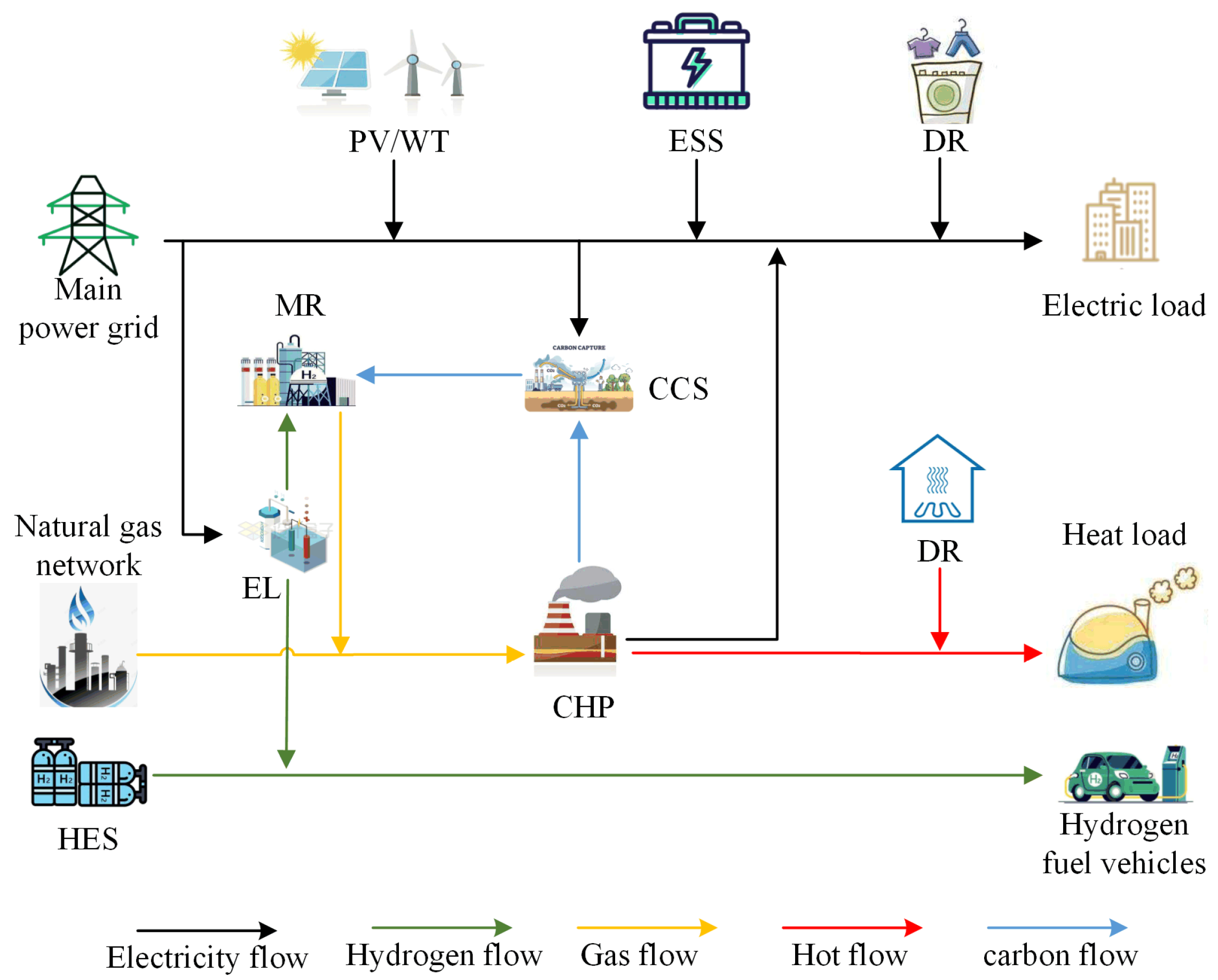
2. MEMG Network Electricity–Hydrogen Shared Operation Architecture

Figure 1 shows the MEMG network’s operation architecture for sharing electricity and hydrogen. A single local controller (LC) collects data on each MG’s energy and load and manages it optimally. To facilitate the trading of energy and hydrogen between MGs, the MEMG aggregator is in charge of receiving and reporting the trading values of electricity and hydrogen between each MG, and protects MG privacy. Meanwhile, the distribution grid and the gas grid provide electricity and natural gas to the MGs to ensure the proper operation of each MG.

In terms of electricity trading, if the MG’s electricity output fails to meet demand, it can try to balance the load by buying electricity from other MGs. If that does not work, it can then buy electricity from the distribution grid to make up the difference. Concerning hydrogen trading, the use of excess renewable energy is prioritized for producing hydrogen through the electrolysis of water. If an MG’s internal hydrogen energy is not enough to meet the demand for hydrogen, purchasing hydrogen from other MGs is the first option. If this is still not enough, purchasing electric energy is required to produce hydrogen.

3. Multi-Energy MG Model

3.1. Multi-Energy MG System Architecture

Figure 2 depicts the energy flow inside the multi-energy MG, which includes renewable energy sources, natural gas-powered CHP units, energy storage systems (ESSs), and demand response (DR) resources. CCSs and P2G are added to conventional CHP units to reduce carbon emissions, with P2G including a water electrolyze (EL), methane reactor (MR), and hydrogen energy storage (HES). Specifically, in the CHP unit part, the gas turbine (GT) and gas boiler (GB) burn natural gas to provide electricity and heat for the system. Meanwhile, the CCS captures and supplies the carbon dioxide created during the CHP unit’s combustion to the P2G. EL prioritizes the use of renewable energy to produce hydrogen energy, with a portion of the hydrogen energy reacting with carbon dioxide captured by the CCS in the MR device to generate natural gas, and the remaining hydrogen energy is stored in HES and supplied to hydrogen fuel vehicles. Meanwhile, ESS, electricity DR, and heat DR are used to alleviate supply and demand pressures. In addition to trading electricity within the distribution network, each MG can also trade hydrogen energy between interconnected MGs. Although gaseous hydrogen pipelines are currently more suitable for long-distance transport, Ref. [40] shows that with maturity in the hydrogen energy market, pipelines gain a cost advantage in hydrogen energy transport. Therefore, this paper considers electricity and hydrogen energy trading among interconnected MGs to enhance the flexibility of energy management in the MEMG network.

3.2. Device Model

3.2.1. CCS-P2G-CHP Model

1.

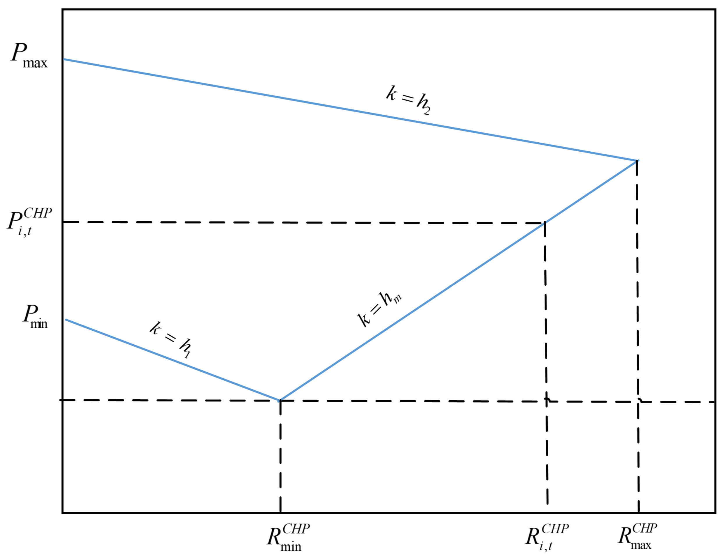
CHP

In the CHP unit, the GT burns natural gas to provide electricity and heat to the system [41].

$$P_{i,t}^{CHP}=V_{i,t}^{CHP}{\eta }_{CHP}{Q}_{C{H}_4}$$

(1)

where $P_{i,t}^{CHP}$ is the electrical energy generated by the GT, $V_{i,t}^{CHP}$ is the consumption of natural gas, ${\eta }_{CHP}$ is the power generation efficiency, and $Q_{C{H}_4}$ is the combustion heat value of natural gas. Considering the cogeneration power of the CHP unit has the constraint of “determining electricity based on heat”, the thermal power $R_{i,t}^{CHP}$ of the GT can be expressed as:

$$\max \{P_{\min }-h_1{R}_{i,t}^{CHP},h_m(R_{i,t}^{CHP}-R_{i,0})\}\le P_{i,t}^{CHP}\le P_{\max }-h_2{R}_{i,t}^{CHP}$$

(2)

where $R_{i,t}^{CHP}$ is the thermal power of the CHP unit, $h_1$ and $h_2$ are the thermoelectric conversion coefficients corresponding to the minimum output power $P_{\min }$ and the maximum output power $P_{\max }$, and $h_m$ is the linear supply slope of the CHP unit thermoelectric power. $R_{i,0}$ is the thermoelectric power corresponding to the lowest generation power of the CHP unit.

Equation (2) describes the constraint conditions for the electric power output $P_{i,t}^{CHP}$ of CHP units, and its upper and lower limits are directly related to the thermal power output $R_{i,t}^{CHP}$, reflecting the principle that “thermal demand determines power output”.

(1)

Left lower limit: determined by the larger of the two parts:

(a)

Weakening of the lower limit of electrical power by thermal power: $P_{\min }-h_1{R}_{i,t}^{CHP}$

When the thermal power $R_{i,t}^{CHP}$ increases, the lower limit of electrical power decreases. This indicates that more fuel is used for heat generation, resulting in limited power generation capacity.

    (b)

Adjustment of thermal power benchmark: $h_m(R_{i,t}^{CHP}-R_{i,0})$

When the thermal power exceeds the reference value $R_{i,0}$, the lower limit of electrical power increases linearly with the thermal power, ensuring that the minimum power generation can still be maintained when the demand for heat generation increases.

(2)

Right upper limit: $P_{\max }-h_2{R}_{i,t}^{CHP}$

When the thermal power $R_{i,t}^{CHP}$ increases, the upper limit of electrical power decreases. When the total amount of fuel is fixed, there is a competitive relationship between heat generation and power generation. The higher the demand for heat generation, the smaller the potential for power generation.

The demand for heat power is the dominant variable, and the feasible range of electrical power is determined by thermal power. Figure 3 shows the domain scope of $R_{i,t}^{CHP}$ and $P_{i,t}^{CHP}$.

The heat generation power $R_{i,t}^{GB}$ of the GB is:

$$R_{i,t}^{GB}=V_{i,t}^{GB}{\eta }_{GB}{Q}_{C{H}_4}$$

(3)

where $V_{i,t}^{GB}$ is the natural gas consumption and ${\eta }_{GB}$ is the heat production efficiency.

In the CHP device with P2G and a CCS, the electricity generated by CHP can be divided into three parts based on its usage:

$$P_{i,t}^{CHP}=P_{i,t}^E+P_{i,t}^{CCS}+P_{i,t}^{P2G}$$

(4)

where $P_{i,t}^E$ is the electricity supplied by the CHP unit to meet the load demand, $P_{i,t}^{CCS}$ and $P_{i,t}^{P2G}$ are the electricity supplied to the CCS and P2G. And the electrical power of CCS, P2G, and CHP should all be within the upper and lower limits:

$$P_{\min }^{CCS}\le P_{i,t}^{CCS}\le P_{\max }^{CCS}$$

(5)

$$P_{\min }^{P2G}<P_{i,t}^{P2G}<P_{\max }^{P2G}$$

(6)

$$P_{\min }^{CHP}\le P_{i,t}^{CHP}\le P_{\max }^{CHP}$$

(7)

where $P_{\min }^{CCS}$ and $P_{\max }^{CCS}$ are the lower and upper limits of CCS power consumption, $P_{\min }^{P2G}$ and $P_{\max }^{P2G}$ are the lower and upper limits of the power consumption of P2G, and $P_{\min }^{CHP}$ and $P_{\max }^{CHP}$ are the lower and upper limits of CHP power generation.

The upper and lower bound constraints of Equations (5) and (6) are substituted into Equation (2) to obtain the electro-thermal coupling characteristic equation for the CHP system containing P2G and a CCS:

$$\max \{P_{\min }^E-h_1{R}_{i,t}^{CHP},h_m(R_{i,t}^{CHP}-R_{i,0})-P_{\max }^{P2G}-P_{\max }^{CCS}\}\le P_{i,t}^E\le P_{\max }^E-h_2{R}_{i,t}^{CHP}-P_{\min }^{P2G}-P_{\min }^{CCS}$$

(8)

2.

CCS

$$P_{i,t}^{CCS}=\gamma W_{i,t}^{P2G}$$

(9)

$$W_{i,t}^{P2G}=\beta P_{i,t}^{P2G}$$

(10)

where $\gamma$ is the conversion coefficient of the electrical energy consumed to capture carbon dioxide, $W_{i,t}^{P2G}$ is the amount of carbon dioxide required for P2G, and $\beta$ is the coefficient used to calculate the amount of carbon dioxide.

3.

P2G

    (a)

EL

$$H_{i,t}^{EL}={\eta }_{H_2}{P}_{i,t}^{P2G}$$

(11)

where $H_{i,t}^{EL}$ is the hydrogen energy output and ${\eta }_{H_2}$ is the hydrogen energy conversion efficiency.

    (b)

MR

$$V_{i,t}^{MR}={\eta }_{MR}{H}_{i,t}^{MR}$$

(12)

where $V_{i,t}^{MR}$ is the natural gas power produced by the MR, ${\eta }_{MR}$ is the conversion efficiency, and $H_{i,t}^{MR}$ is the hydrogen energy consumed by the MR.

    (c)

HES

$$HE{S}_{i,t}=HE{S}_{i,t-1}(1-{\sigma }_{HS})+H_{i,t}^{HSC}{\eta }_{HSC}-H_{i,t}^{HSD}{\eta }_{HSD}$$

(13)

$$HE{S}_{\min }\le HE{S}_{i,t}\le HE{S}_{\max }$$

(14)

$$0\le H_{i,t}^{HSC}\le U_{i,t}^{HSC}{H}_{\max }^{HSC}$$

(15)

$$0\le H_{i,t}^{HSD}\le U_{i,t}^{HSD}{H}_{\max }^{HSD}$$

(16)

$$U_{i,t}^{HSC}+U_{i,t}^{HSD}\le 1$$

(17)

$HE{S}_{i,t}$ is the hydrogen energy stored in HES, $H_{i,t}^{HSC}$ and $H_{i,t}^{HSD}$ represent the hydrogen energy charged and discharged, ${\sigma }_{HS}$ represents the rate of self-consumption, and ${\eta }_{HSC}$ and ${\eta }_{HSD}$ are the efficiencies of charging and discharging. $HE{S}_{\min }$ and $HE{S}_{\max }$ are the minimum and maximum hydrogen energy stored. $H_{\max }^{HSC}$ and $H_{\max }^{HSD}$ represent the maximum amount of charging and discharging. $U_{i,t}^{HSC}$ and $U_{i,t}^{HSD}$ represent the state of charging and discharging, which takes the value of 1 for charging and 0 for discharging.

3.2.2. ESS

Equation (18) is the charging state of the ESS, $E_{i,t}^e$ is the electrical energy stored in the ESS, ${\eta }_{loss}$ is the energy loss coefficient, $\eta$ is the charging and discharging efficiencies, and $P_{i,t}^{cha}$ and $P_{i,t}^{dis}$ are the charging and discharging powers. $E_{\min }^e$ and $E_{\max }^e$ are the minimum and maximum residual capacities. $E_{i,0}^e$ and $E_{i,24}^e$ are the stored energy of the ESS at the beginning and end moments. $P_{\max }^{cha}$ and $P_{\max }^{dis}$ are the upper limits of the charging and discharging power, and $U_{i,t}^{ess}$ represents the charging and discharging states, which take the value of 1 for charging and 0 for discharging.

$$E_{i,t}^e=(1-{\eta }_{loss})E_{i,t-1}^e+(\eta P_{i,t}^{cha}-{\displaystyle \frac{1}{\eta }}{P}_{i,t}^{dis})\Delta t$$

(18)

$$E_{\min }^e\le E_{i,t}^e\le E_{\max }^e$$

(19)

$$E_{i,0}^e=E_{i,24}^e=20\%E_{\max }^e$$

(20)

$$0\le P_{i,t}^{cha}\le U_{i,t}^{ess}{P}_{\max }^{cha}$$

(21)

$$0\le P_{i,t}^{dis}\le (1-U_{i,t}^{ess})P_{\max }^{dis}$$

(22)

$$U_{i,t}^{cha}+U_{i,t}^{dis}\le 1$$

(23)

3.2.3. DR

The actual electrical load $P_{i,t}^{load}$ within the MG consists of three parts: fixed electrical load $P_{i,t}^f$, translatable electrical load $P_{i,t}^{tran}$, and curtailable electrical load $P_{i,t}^{cut}$, which can be expressed as [42]:

$$P_{i,t}^{load}=P_{i,t}^f+P_{i,t}^{tran}-P_{i,t}^{cut}$$

(24)

$$0\le P_{i,t}^{cut}\le P_{i,\max }^{cut}$$

(25)

$$\left|{\displaystyle \sum _{t=1}^T{P}_{i,t}^{tran}\Delta t}\right|\le k^{tran}{P}_{i,t}^{load}$$

(26)

where $P_{i,\max }^{cut}$ represents the upper limit of the curtailable electrical load, $k^{tran}$ represents the electricity load coefficient that can be transferred.

The actual heat load $R_{i,t}^{load}$ inside the MG consists of two parts: fixed heat load $R_{i,t}^f$ and curtailable heat load $R_{i,t}^{cut}$, which can be expressed as:

$$R_{i,t}^{load}=R_{i,t}^f-R_{i,t}^{cut}$$

(27)

$$0\le R_{i,t}^{cut}\le R_{i,\max }^{cut}$$

(28)

$R_{i,\max }^{cut}$ represents the upper limit of the curtailable heat load.

3.3. Theoretical Model

3.3.1. Objective Function

The cost of a multi-energy MG considering electricity–hydrogen sharing can be expressed as:

$$\min C_i^{MG}=C_i^{CHP}+C_i^{utility}+C_i^{ESS}+C_i^{HES}+C_i^{C{O}_2}+C_i^{DR}+C_i^{tran,e}+C_i^{P2P,e}+C_i^{tran,h}+C_i^{P2P,h}$$

(29)

(1)

Operating costs of CHP units $C_i^{CHP}$

$$C_i^{CHP}={\displaystyle \sum _{t=1}^T[a_1{P}_{i,t}^E+b_1{(P_{i,t}^E)}^2+a_2{P}_{i,t}^{CCS}+a_3{P}_{i,t}^{P2G}]}$$

(30)

where $a_1$ and $b_1$ are the operating cost coefficients of the CHP; $a_2$ and $a_3$ are the operating cost coefficients of CCS and P2G.

(2)

External interaction cost $C_i^{utility}$

$$C_i^{utility}={\displaystyle \sum _{t=1}^T[({\lambda }_{i,t}^{C{H}_4}{V}_{i,t}^{buy})+({\lambda }_{i,t}^{buy}{P}_{i,t}^{buy}-{\lambda }_{i,t}^{sell}{P}_{i,t}^{sell})]}$$

(31)

where ${\lambda }_{i,t}^{C{H}_4}$ and $V_{i,t}^{buy}$ are the purchase prices and amount of natural gas. ${\lambda }_{i,t}^{buy}$ and $P_{i,t}^{buy}$ represent the purchase price and amount of electricity, while ${\lambda }_{i,t}^{sell}$ and $P_{i,t}^{sell}$ represent the sale price and amount of electricity.

(3)

Operational degradation cost of ESS

$$C_{i,e}^{ESS}={\displaystyle \sum _{t=1}^T{\varsigma }_e(P_{i,t}^{cha}+P_{i,t}^{dis})}$$

(32)

where ${\varsigma }_e$ represents the unit degradation cost of charging and discharging.

(4)

Operational degradation cost of HES

$$C_i^{HES}={\displaystyle \sum _{t=1}^T{c}_{HS}H{S}_{i,t}}$$

(33)

where $c_{HS}$ is the cost coefficient of self-consumption,

(5)

Carbon trading costs

$$W_{i,t}^0=D(P_{i,t}^{CHP}+P_{i,t}^{PV}+P_{i,t}^{WT})$$

(34)

where $W_{i,t}^0$ is the initial carbon quota, $D$ is the carbon emission quota per unit of electricity production; $P_{i,t}^{PV}$ and $P_{i,t}^{WT}$ represent the power generated by photovoltaic (PV) and wind turbine (WT) sources.

$$W_{i,t}^{c{o}_2}=a_{c{o}_2}(P_{i,t}^e+h_1{R}_{i,t}^{CHP})+b_{c{o}_2}{R}_{i,t}^{GB}+c_{c{o}_2}-C_{cc,t}$$

(35)

where $W_{i,t}^{c{o}_2}$ is the carbon dioxide emissions,$a_{c{o}_2}$. $b_{c{o}_2}$ and $c_{c{o}_2}$ are the carbon dioxide emission coefficients of the CHP units and GB [43,44]; $C_{cc,t}$ is the carbon dioxide emissions captured by the CCS.

The carbon trading cost $C_i^{C{O}_2}$ is expressed as:

$$C_i^{C{O}_2}={\displaystyle \sum _{t=1}^T\epsilon (W_{i,t}^{C{O}_2}-W_{i,t}^0)}$$

(36)

where $\epsilon$ is the carbon trading cost coefficient.

(6)

DR cost

$$C_i^{DR}={\displaystyle \sum _{t=1}^T({\lambda }_e^{cut}{P}_{i,t}^{cut}+{\lambda }_e^{tran}{P}_{i,t}^{tran}+{\lambda }_r^{cut}{R}_{i,t}^{cut})}$$

(37)

where ${\lambda }_e^{cut}$, ${\lambda }_e^{tran}$, and ${\lambda }_r^{cut}$ are the compensation cost coefficients for the curtailable and translatable electrical loads and curtailable heat loads.

(7)

Electricity transmission cost $C_i^{tran.e}$

$$C_i^{tran.e}={\displaystyle \sum _{t=1}^T{\displaystyle \sum _{j\ne i}^I{a}_e{P}_{ij,t}^{P2P}}}$$

(38)

where $a_e$ represents the transmission cost of unit electricity across the distribution network. The coalition set within the MG is defined as $I$. $P_{ij,t}^{P2P}$ denotes the amount of electricity traded between $M{G}_i$ and $M{G}_j$. If $P_{ij,t}^{P2P}>0$, $M{G}_i$ obtains electricity from $M{G}_j$, otherwise, it supplies electricity to $M{G}_j$.

(8)

Electricity trading cost $C_i^{P2P,e}$

$$C_i^{P2P,e}={\displaystyle \sum _{t=1}^T{\displaystyle \sum _{j\ne i}^I{r}_{ij,t}^{P2P,e}{P}_{ij,t}^{P2P}}}$$

(39)

where $r_{ij,t}^{P2P,e}$ represents the price of electricity trading between $M{G}_i$ and $M{G}_j$.

(9)

Hydrogen energy transmission cost $C_i^{tran,h}$

$$C_i^{tran,h}={\displaystyle \sum _{t=1}^T{\displaystyle \sum _{j\ne i}^I{a}_h{H}_{ij,t}^{P2P}}}$$

(40)

where $a_h$ represents the transportation cost per unit of hydrogen energy and $H_{ij,t}^{P2P}$ represents the hydrogen energy trading amount between $M{G}_i$ and $M{G}_j$. If $H_{ij,t}^{P2P}>0$, $M{G}_i$ obtains hydrogen energy from $M{G}_j$; otherwise, it supplies hydrogen energy to $M{G}_j$.

(10)

Hydrogen energy trading cost $C_i^{P2P,h}$

$$C_i^{P2P,h}={\displaystyle \sum _{t=1}^T{\displaystyle \sum _{j\ne i}^I{r}_{ij,t}^{P2P,h}{H}_{ij,t}^{P2P}}}$$

(41)

where $r_{ij,t}^{P2P,h}$ represents the trading price of hydrogen energy.

3.3.2. Constraints

(1)

Power balance constraint

$$P_{i,t}^{PV}+P_{i,t}^{WT}+P_{i,t}^E+P_{i,t}^{CCS}+P_{i,t}^{P2G}+P_{i,t}^{buy}+P_{i,t}^{dis}=P_{i,t}^{load}+P_{i,t}^{cha}+P_{i,t}^{sell}+P_{ij,t}^{P2P}$$

(42)

(2)

Heat power balance constraint

$$R_{i,t}^{CHP}+R_{i,t}^{GB}=R_{i,t}^{load}$$

(43)

where $R_{i,t}^{load}$ is the heat load.

(3)

Hydrogen energy balance constraint

$$H_{i,t}^{EL}+H_{i,t}^{HSC}=H_{i,t}^{load}+H_{i,t}^{MR}+H_{i,t}^{HSD}$$

(44)

where $H_{i,t}^{load}$ is the hydrogen energy load.

(4)

Natural gas balance constraint

$$V_{i,t}^{buy}=V_{i,t}^{CHP}+V_{i,t}^{GB}-V_{i,t}^{MR}$$

(45)

(5)

Electricity trading constraints

$$\left|P_{ij,t}^{P2P}\right|\le P_{ij,\max }^{P2P}$$

(46)

$P_{ij,\max }^{P2P}$ is the limit of electrical energy trading power; let $P_{i,t}^{P2P}$ represent the total electricity trading amount of $M{G}_i$, corresponding to the total transaction fee that needs to be paid as $v_{i,t}^e$. $M{G}_i$ participating in electricity trading must meet the constraints of energy sharing balance and transaction payment balance:

$${\displaystyle \sum _{i\in I}{P}_{i,t}^{P2P}=0,\forall t}$$

(47)

$${\displaystyle \sum _{i\in I}{v}_{i,t}^e=0,\forall t}$$

(48)

(6)

Hydrogen trading constraints

$$\left|H_{ij,t}^{P2P}\right|\le H_{ij,\max }^{P2P}$$

(49)

$H_{ij,\max }^{P2P}$ is the limit of hydrogen energy transfer; let $H_{i,t}^{P2P}$ represent the total hydrogen energy trading amount of $M{G}_i$ corresponding to the total transaction fee that needs to be paid as $v_{i,t}^h$. $M{G}_i$ participating in hydrogen energy trading must meet the constraints of energy sharing balance and transaction payment balance:

$${\displaystyle \sum _{i\in I}{H}_{i,t}^{P2P}=0,\forall t}$$

(50)

$${\displaystyle \sum _{i\in I}{v}_{i,t}^h=0,\forall t}$$

(51)

3.4. Linearization of the Uncertainty Model for PV and WT Output

This study uses robust intervals to describe the uncertainty range of renewable energy output, as follows:

$$P_{PV}(t)=[{\overline{P}}_{PV}(t)-P_{PV}^{ld},{\overline{P}}_{PV}(t)+P_{PV}^{ud}]$$

(52)

$$P_{WT}(t)=[{\overline{P}}_{WT}(t)-P_{WT}^{ld},{\overline{P}}_{WT}(t)+P_{WT}^{ud}]$$

(53)

Among them, $P_{PV}(t)$ and $P_{WT}(t)$ are the actual output of PV and WT power, ${\overline{P}}_{PV}(t)$ and ${\overline{P}}_{WT}(t)$ are the predicted values of PV and WT power, and $P_{PV}^{ld},P_{PV}^{ud},P_{WT}^{ld},P_{WT}^{ud}$ represents the maximum allowable deviation of PV and WT output, respectively. Based on the robust optimization method proposed in Ref. [45], an analytical expression for the worst-case power balance constraint is constructed, as follows:

$$\begin{array}{c}{P}_{i,t}^{load}=\max P_{i,t}^{PV}+\max P_{i,t}^{WT}+P_{i,t}^E+P_{i,t}^{CCS}+P_{i,t}^{P2G}+P_{i,t}^{dis}+P_{i,t}^{buy}-P_{i,t}^{cha}-P_{i,t}^{sell}-P_{ij,t}^{P2P}\\ ={\overline{P}}_{PV}(t)+{\overline{P}}_{WT}(t)+\max \{{\eta }_{PV}^{ld}{P}_{PV}^{ld}+{\eta }_{PV}^{ud}{P}_{PV}^{ud}+{\eta }_{WT}^{ld}{P}_{WT}^{ld}+{\eta }_{WT}^{ud}{P}_{WT}^{ud}\}\\ +P_{i,t}^E+P_{i,t}^{CCS}+P_{i,t}^{P2G}+P_{i,t}^{dis}+P_{i,t}^{buy}-P_{i,t}^{cha}-P_{i,t}^{sell}-P_{ij,t}^{P2P}\end{array}$$

(54)

$${\eta }_{PV}^{ld}+{\eta }_{PV}^{ud}+{\eta }_{WT}^{ld}+{\eta }_{WT}^{ud}\le {\Gamma }_t$$

(55)

$$0\le {\eta }_{PV}^{ld},{\eta }_{PV}^{ud},{\eta }_{WT}^{ld},{\eta }_{WT}^{ud}\le 1$$

(56)

Among them, ${\eta }_{PV}^{ld},{\eta }_{PV}^{ud},{\eta }_{WT}^{ld},{\eta }_{WT}^{ud}$ represents the proportional deviation of PV and WT power output relative to its fluctuation range, and ${\Gamma }_t$ represents the uncertainty of the model.

In order to obtain a solvable form of the above problem, a dual variable ${\lambda }_{PV}^t,{\lambda }_{WT}^t,{\pi }_{PV}^{t+},{\pi }_{PV}^{t-},{\pi }_{WT}^{t+},{\pi }_{WT}^{t-}$ is introduced, as shown in Equations (57)–(61):

$$\min {\lambda }_{PV}^t{\Gamma }_{PV}^t+{\pi }_{PV}^{t+}+{\pi }_{PV}^{t-}+{\lambda }_{WT}^t{\Gamma }_{WT}^t+{\pi }_{WT}^{t+}+{\pi }_{WT}^{t+}$$

(57)

$${\lambda }_{PV}^t+{\pi }_{PV}^{t+}\ge P_{PV}^{ud}$$

(58)

$${\lambda }_{PV}^t+{\pi }_{PV}^{t-}\ge P_{PV}^{ld}$$

(59)

$${\lambda }_{WT}^t+{\pi }_{WT}^{t+}\ge P_{WT}^{ud}$$

(60)

$${\lambda }_{WT}^t+{\pi }_{WT}^{t-}\ge P_{WT}^{ld}$$

(61)

In summary, the model raised in this paper can be expressed by (1)–(51) and (57)–(61).

4. MEMG Electricity–Hydrogen Sharing Optimization Model Based on Asymmetric Nash Bargaining

4.1. Nash Bargaining Problem

The NB model used in this paper is a cooperative game. Assuming that each MG acts independently and rationally in external transactions and can minimize its own operational expenses by participating in bargaining, the standard model of NB can be expressed as follows [46].

$$\max {\displaystyle \prod _{i=1}^I(C_i^0-C_i^{MG}})$$

(62)

$$C_i^0-C_i^{MG}\ge 0$$

(63)

where $C_i^0$ is the point of negotiation breakdown, which does not consider the cost of energy sharing between MGs. $C_i^{MG}$ is the utility function for participating in energy sharing. $C_i^0-C_i^{MG}$ is the payment benefit that the MG receives through energy sharing. The bargaining strategy for each MG is $\{r_{ij,t}^{P2P,e},P_{ij,t}^{P2P},r_{ij,t}^{P2P,h},H_{ij,t}^{P2P}\}$. By solving the equilibrium solution of Equation (62), each MG can solve the optimal bargaining strategy and achieve the minimization of operating cost.

4.2. Equivalent Transformation of Problems

Since both the trading price and amount are included as optimization variables in Equation (62), which is effectively a non-convex non-linearization problem. This study transforms Equation (62) into two easily solvable subproblems: minimization of the MEMG network cost and maximization of the payment benefit, and obtains the optimal solution to the original problem through sequential optimization.

Subproblem 1: minimization of the MEMG network cost.

$$\max -{\displaystyle \prod _{i=1}^I{C}_i^{M{G}^{\prime }}}$$

(64)

where $C_i^{M{G}^{\prime }}=C_i^{CHP}+C_i^{utility}+C_i^{ESS}+C_i^{HES}+C_i^{C{O}_2}+C_i^{DR}+C_i^{tran,e}+C_i^{tran,h}$

Subproblem 2: maximization of the payment benefit.

Subproblem 2 studies the distribution of benefits to the MGs after energy sharing. ANB is an economic term that refers to the fact that negotiation parties have different bargaining power as a result of information or position asymmetry [47]. This study determines the contribution based on the amount of electricity and hydrogen energy trading between each MG. The MGs then utilize their contributions as bargaining power to negotiate the energy trading price, as well as the equitable distribution of energy trading benefits. The expression is as follows:

$$d_i={\gamma }_e{\displaystyle \frac{{\displaystyle \sum _{j=1,j\ne i}^I{\displaystyle \sum _{t=1}^T\left|P_{ij,t}^{P2P}\right|}}}{{\displaystyle \sum _{i=1}^I{\displaystyle \sum _{j=1,j\ne i}^I{\displaystyle \sum _{t=1}^T\left|P_{ij,t}^{P2P}\right|}}}}}+{\gamma }_h{\displaystyle \frac{{\displaystyle \sum _{j=1,j\ne i}^I{\displaystyle \sum _{t=1}^T\left|H_{ij,t}^{P2P}\right|}}}{{\displaystyle \sum _{i=1}^I{\displaystyle \sum _{j=1,j\ne i}^I{\displaystyle \sum _{t=1}^T\left|H_{ij,t}^{P2P}\right|}}}}}$$

(65)

${\gamma }_e$ and ${\gamma }_h$ represent the weights of electricity and hydrogen energy trading, and satisfying ${\gamma }_e+{\gamma }_h=1$. The expression includes the following elements: (1) Each MG trading electricity and hydrogen energy gains bargaining power. (2) If the MG fails to trade any electricity or hydrogen, its contribution, as well as the profit distribution, are both zero. (3) As the MG’s contribution increases, so does its bargaining power and profit distribution.

The ANB benefits allocation model is as follows:

$$\begin{array}{l}\max {{\displaystyle \prod _{i=1}^I(C_i^0-C_i^{M{G}^{\prime }}+C_i^{P2P,e}+C_i^{P2P,h})}}^{d_i}\\ s.t.(50)-(51)\end{array}$$

(66)

$$C_i^0-C_i^{M{G}^{\prime }}+C_i^{P2P,e}+C_i^{P2P,h}>0$$

(67)

Taking the logarithm of Equation (66) changes the maximization problem to a minimization problem for ease of solution, as shown below:

$$\min {\displaystyle \prod _{i=1}^I-d_i\ln (C_i^0-C_i^{M{G}^{\prime }}+C_i^{P2P,e}+C_i^{P2P,h})}$$

(68)

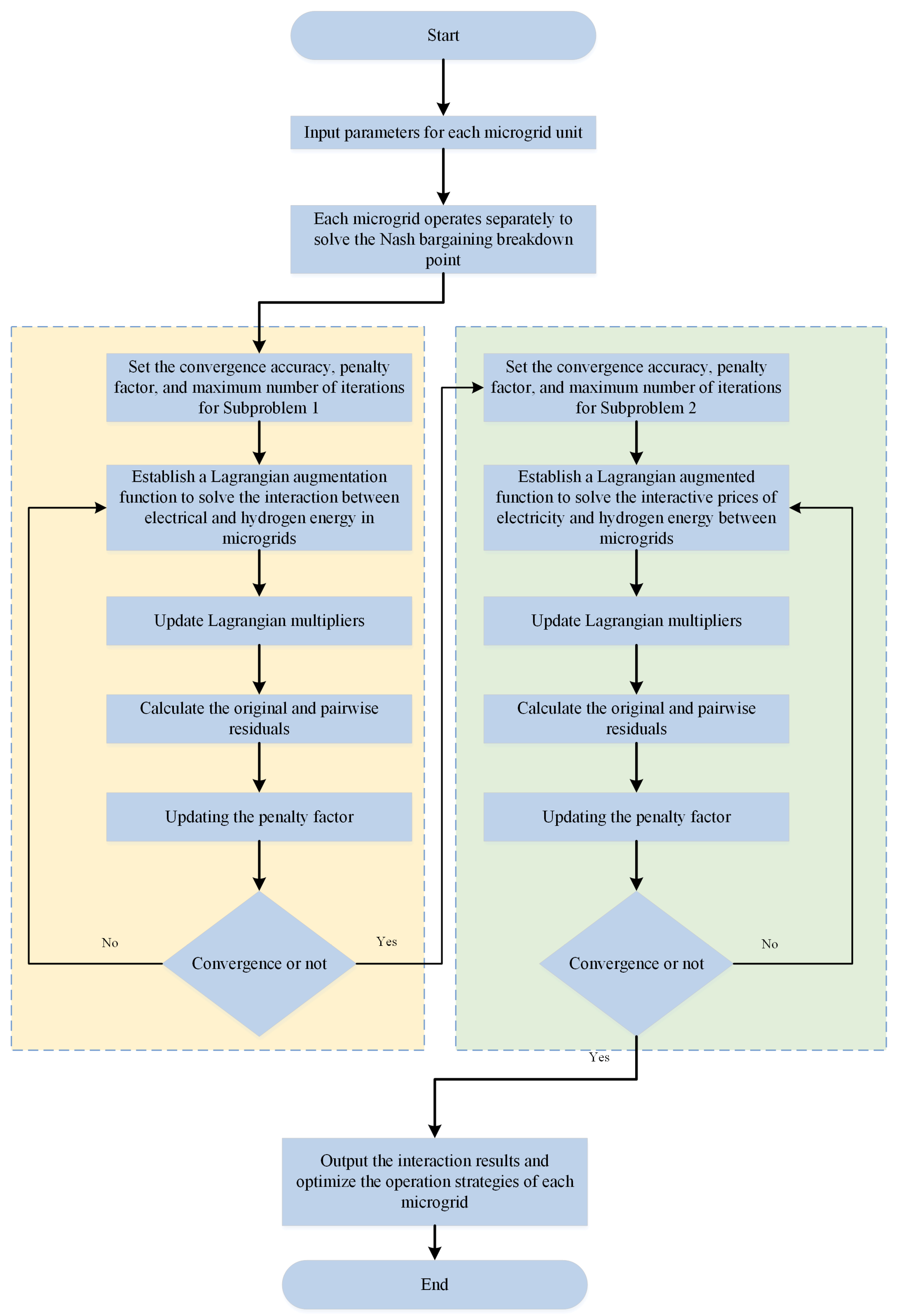
5. Model Solution

5.1. Improved ADMM Algorithm

The traditional ADMM is prone to sluggish convergence because of the fixed penalty factor $\rho$. This study automatically updates the penalty factor by comparing the size of the original residual and the dual residual, avoiding the algorithm from falling into local optima or converging too fast [6]. The dynamic penalty factor is expressed as follows:

$$\rho (k+1)=\left\{\begin{array}{c}{\vartheta }_1\rho (k), {‖r(k)‖}_2>\mu {‖s(k)‖}_2\\ \begin{array}{l}\rho (k)/{\vartheta }_2, {‖s(k)‖}_2>\mu {‖r(k)‖}_2\\ \rho (k),\mathrm{else}\end{array}\end{array}\right.$$

(69)

where $r(k)$ and $s(k)$ are the original and pairwise residual, $\mu >1$ is the scale factor of $r(k)$ and $s(k)$, ${\vartheta }_1$ and ${\vartheta }_2$ are the accelerated and decelerated convergence coefficients, and ${\vartheta }_1>1,{\vartheta }_2>1$ is satisfied.

5.2. Solution to Subproblem 1

(1)

The electricity trading $P_{ij,t}^{P2P}$ and the hydrogen energy trading $H_{ij,t}^{P2P}$ are coupled variables satisfying $P_{ij,t}^{P2P}=-P_{ji,t}^{P2P}$ and $H_{ij,t}^{P2P}=-H_{ji,t}^{P2P}$. Therefore, the MG augmented Lagrange function for subproblem 1 can be expressed as follows:

$$\begin{array}{l}{L}_i^{P1}(P_{ij,t}^{P2P},P_{ji,t}^{P2P},H_{ij,t}^{P2P},H_{ij,t}^{P2P},{\lambda }_{ij}^{P1,e},{\lambda }_{ij}^{P1,h})=C_i^{M{G}^{‘}}+{\displaystyle \sum _h^{h+23}{\displaystyle \sum _{i\in I/i}[\frac{{\rho }_{ij}^{P1,e}}{2}{‖P_{ij,t}^{P2P}+P_{ji,t}^{P2P}‖}_2^2+{\lambda }_{ij}^{P1,e}(P_{ij,t}^{P2P}+P_{ji,t}^{P2P})]}}\\ +{\displaystyle \sum _h^{h+23}{\displaystyle \sum _{i\in I/i}[\frac{{\rho }_{ij}^{P1,h}}{2}{‖H_{ij,t}^{P2P}+H_{ij,t}^{P2P}‖}_2^2+{\lambda }_{ij}^{P1,h}(H_{ij,t}^{P2P}+H_{ij,t}^{P2P})]}}\end{array}$$

(70)

where ${\lambda }_{ij}^{P1,e}$ and ${\lambda }_{ij}^{P1,h}$ are the Lagrange factors, and ${\rho }_{ij}^{P1,e}$ and ${\rho }_{ij}^{P1,h}$ are the penalty factors.

(2)

$M{G}_i$ updates its own energy trading strategy.

$$P_{ij,t}^{P2P}(k+1)=\arg \min L_i^{P1}(P_{ij,t}^{P2P}(k),P_{ji,t}^{P2P}(k),{\lambda }_{ij}^{P1,e}(k))$$

(71)

$$H_{ij,t}^{P2P}(k+1)=\arg \min L_i^{P1}(H_{ij,t}^{P2P}(k),H_{ji,t}^{P2P}(k),{\lambda }_{ij}^{P1,h}(k))$$

(72)

$M{G}_j$ receives updated decision information $P_{ij,t}^{P2P}(k+1)$ and $H_{ij,t}^{P2P}(k+1)$ to update their decisions for $P_{ji,t}^{P2P}(k+1)$ and $H_{ji,t}^{P2P}(k+1)$.

$$P_{ji,t}^{P2P}(k+1)=\arg \min L_i^{P1}(P_{ji,t}^{P2P}(k),P_{ij,t}^{P2P}(k+1),{\lambda }_{ji}^{P1,e}(k))$$

(73)

$$H_{ji,t}^{P2P}(k+1)=\arg \min L_i^{P1}(H_{ji,t}^{P2P}(k),H_{ij,t}^{P2P}(k+1),{\lambda }_{ji}^{P1,h}(k))$$

(74)

Repeat the computation of Equations (71)–(74) until each MG updates its trading strategy in the current iteration.

(3)

Lagrange multipliers are updated as a rule.

$${\lambda }_{ij}^{P1,e}(k+1)={\lambda }_{ij}^{P1,e}(k)+{\rho }_{ij}^{P1,e}(k)(P_{ij,t}^{P2P}(k)+P_{ji,t}^{P2P}(k))$$

(75)

$${\lambda }_{ij}^{P1,h}(k+1)={\lambda }_{ij}^{P1,h}(k)+{\rho }_{ij}^{P1,h}(k)(H_{ij,t}^{P2P}(k)+H_{ji,t}^{P2P}(k))$$

(76)

(4)

Calculate the original residual and pairwise residual, and update the penalty factor according to Equation (69).

$$\begin{array}{l}{r}_{ij}^{P1,e}(k)={\displaystyle \sum _{t=1}^T{P}_{ij,t}^{P2P}(k)+P_{ji,t}^{P2P}(k)}; r_{ij}^{P1,h}(k)={\displaystyle \sum _{t=1}^T{H}_{ij,t}^{P2P}(k)+H_{ji,t}^{P2P}(k)}\\ s_{ij}^{P1,e}(k)={\displaystyle \sum _{t=1}^T{P}_{ij,t}^{P2P}(k+1)-P_{ij,t}^{P2P}(k)}; s_{ij}^{P1,h}(k)={\displaystyle \sum _{t=1}^T{H}_{ij,t}^{P2P}(k+1)-H_{ij,t}^{P2P}(k)}\end{array}$$

(77)

where $r_{ij}^{P1,e}(k)$ and $s_{ij}^{P1,e}(k)$ are the residual and pairwise residuals of the electricity trading, and $r_{ij}^{P1,h}(k)$ and $s_{ij}^{P1,h}(k)$ are the residual and pairwise residuals of the hydrogen energy trading.

(5)

Determining the convergence of the algorithm

$$\left\{\begin{array}{l}{‖r_{ij}^{P1,e}(k)‖}_2<{\epsilon }_1\\ {‖s_{ij}^{P1,e}(k)‖}_2<{\epsilon }_2\end{array}\right., \left\{\begin{array}{l}{‖r_{ij}^{P1,h}(k)‖}_2<{\epsilon }_1\\ {‖s_{ij}^{P1,h}(k)‖}_2<{\epsilon }_2\end{array}\right.$$

(78)

${\epsilon }_1$ is the original residual convergence threshold and ${\epsilon }_2$ is the pairwise residual convergence threshold. If Equation (78) is satisfied, the iteration is terminated, otherwise return to step (2) to enter the next round of iteration until the convergence condition is satisfied.

5.3. Solution to Subproblem 2

(1)

Calculate the bargaining power $d_i$ of each MG;

(2)

The electricity trading price $r_{ij,t}^{P2P,e}$ and the hydrogen trading price $r_{ij,t}^{P2P,h}$ are coupled variables satisfying $r_{ij,t}^{P2P,e}=r_{ji,t}^{P2P,e}$ and $H_{ij,t}^{P2P,h}=H_{ji,t}^{P2P,h}$; therefore, the MG’s augmented Lagrange function of subproblem 2 can be expressed as follows.

$$\begin{array}{l}{L}_i^{P2}=-d_i\ln (C_i^0-C_i^{M{G}^{\prime }}+C_i^{P2P,e}+C_i^{P2P,h})+{\displaystyle \sum _{j=1}^I{\displaystyle \sum _{t=1}^T{\lambda }_{ij}^{P2,e}}(r_{ij,t}^{P2P,e}-r_{ji,t}^{P2P,e})+{\displaystyle \sum _{j=1}^I\frac{{\rho }_{ij}^{P2,e}}{2}}{\displaystyle \sum _{t=1}^T{‖r_{ij,t}^{P2P,e}-r_{ji,t}^{P2P,e}‖}_2^2}}\\ +{\displaystyle \sum _{j=1}^I{\displaystyle \sum _{t=1}^T{\lambda }_{ij}^{P2,h}}(r_{ij,t}^{P2P,h}-r_{ji,t}^{P2P,h})+{\displaystyle \sum _{j=1}^I\frac{{\rho }_{ij}^{P2,h}}{2}}{\displaystyle \sum _{t=1}^T{‖r_{ij,t}^{P2P,h}-r_{ji,t}^{P2P,h}‖}_2^2}}\end{array}$$

(79)

where ${\lambda }_{ij}^{P2,e}$ and ${\lambda }_{ij}^{P2,h}$ are the Lagrange factors for subproblem 2, and ${\rho }_{ij}^{P2,e}$ and ${\rho }_{ij}^{P2,h}$ are the penalty factors.

(3)

$M{G}_i$ updates its own price strategy for trading electricity and hydrogen energy.

$$r_{ij,t}^{P2P,e}(k+1)=\arg \min L_i^{P2}(r_{ij,t}^{P2P,e}(k),r_{ji,t}^{P2P,e}(k),{\lambda }_{ij}^{P2,e}(k))$$

(80)

$$r_{ij,t}^{P2P,h}(k+1)=\arg \min L_i^{P2}(r_{ij,t}^{P2P,h}(k),r_{ji,t}^{P2P,h}(k),{\lambda }_{ij}^{P2,h}(k))$$

(81)

$M{G}_j$ receives updated decision information $r_{ij,t}^{P2P,e}(k+1)$ and $r_{ij,t}^{P2P,h}(k+1)$ to update their decisions $r_{ji,t}^{P2P,e}(k+1)$ and $r_{ji,t}^{P2P,h}(k+1)$.

$$r_{ji,t}^{P2P,e}(k+1)=\arg \min L_i^{P2}(r_{ji,t}^{P2P,e}(k),r_{ij,t}^{P2P,e}(k+1),{\lambda }_{ji}^{P2,e}(k))$$

(82)

$$r_{ji,t}^{P2P,h}(k+1)=\arg \min L_i^{P2}(r_{ji,t}^{P2P,h}(k),r_{ij,t}^{P2P,h}(k+1),{\lambda }_{ji}^{P2,h}(k))$$

(83)

Repeat the computation of Equations (80)–(83) until each MG updates its trading strategy in the current iteration.

(4)

Lagrange multipliers are updated as a rule.

$${\lambda }_{ij,e}^{P2}(k+1)={\lambda }_{ij,e}^{P2}(k)+{\rho }_{ij}^{P2,e}(k)(r_{ij,t}^{P2P,e}(k)-r_{ji,t}^{P2P,e}(k))$$

(84)

$${\lambda }_{ij,h}^{P2}(k+1)={\lambda }_{ij,h}^{P2}(k)+{\rho }_{ij}^{P2,h}(k)(r_{ij,t}^{P2P,h}(k)-r_{ji,t}^{P2P,h}(k))$$

(85)

(5)

Calculate the original residual and pairwise residual, and update the penalty factor according to Equation (69).

$$\begin{array}{l}{r}_{ij}^{P2,e}(k)={\displaystyle \sum _{t=1}^T{r}_{ij,t}^{P2P,e}(k)-r_{ji,t}^{P2P,e}(k); r_{ij}^{P2,h}(k)={\displaystyle \sum _{t=1}^T{r}_{ij,t}^{P2P,h}(k)-r_{ji,t}^{P2P,h}(k)}}\\ s_{ij}^{P2,P1,e}(k)={\displaystyle \sum _{t=1}^T{r}_{ij,t}^{P2P,e}(k+1)-r_{ij,t}^{P2P,e}(k)}; s_{ij}^{P2,h}(k)={\displaystyle \sum _{t=1}^T{r}_{ij,t}^{P2P,h}(k+1)-r_{ij,t}^{P2P,h}(k)}\end{array}$$

(86)

where $r_{ij}^{P2,e}(k)$ and $s_{ij}^{P2,e}(k)$ are the residual and pairwise residuals of the electricity price, and $r_{ij}^{P2,h}(k)$ and $s_{ij}^{P2,h}(k)$ are the residual and pairwise residuals of the hydrogen energy price.

(6)

Determining the convergence of the algorithm

$$\left\{\begin{array}{l}{\displaystyle \sum _{i=1}^I{‖r_{ij}^{P2,e}(k)‖}_2\le {\delta }_1}\\ {\displaystyle \sum _{i=1}^I{‖s_{ij}^{P2,e}(k)‖}_2\le {\delta }_2}\end{array}\right., \left\{\begin{array}{l}{\displaystyle \sum _{i=1}^I{‖r_{ij}^{P2,h}(k)‖}_2\le {\delta }_1}\\ {\displaystyle \sum _{i=1}^I{‖s_{ij}^{P2,h}(k)‖}_2\le {\delta }_2}\end{array}\right.$$

(87)

${\delta }_1$ is the original residual convergence threshold and ${\delta }_2$ is the pairwise residual convergence threshold. If Equation (87) is satisfied, the iteration is terminated, otherwise return to step (2) to enter the next round of iteration until the convergence condition is satisfied.

The algorithm flowchart can be seen in Appendix A, Figure A1.

6. Case Study

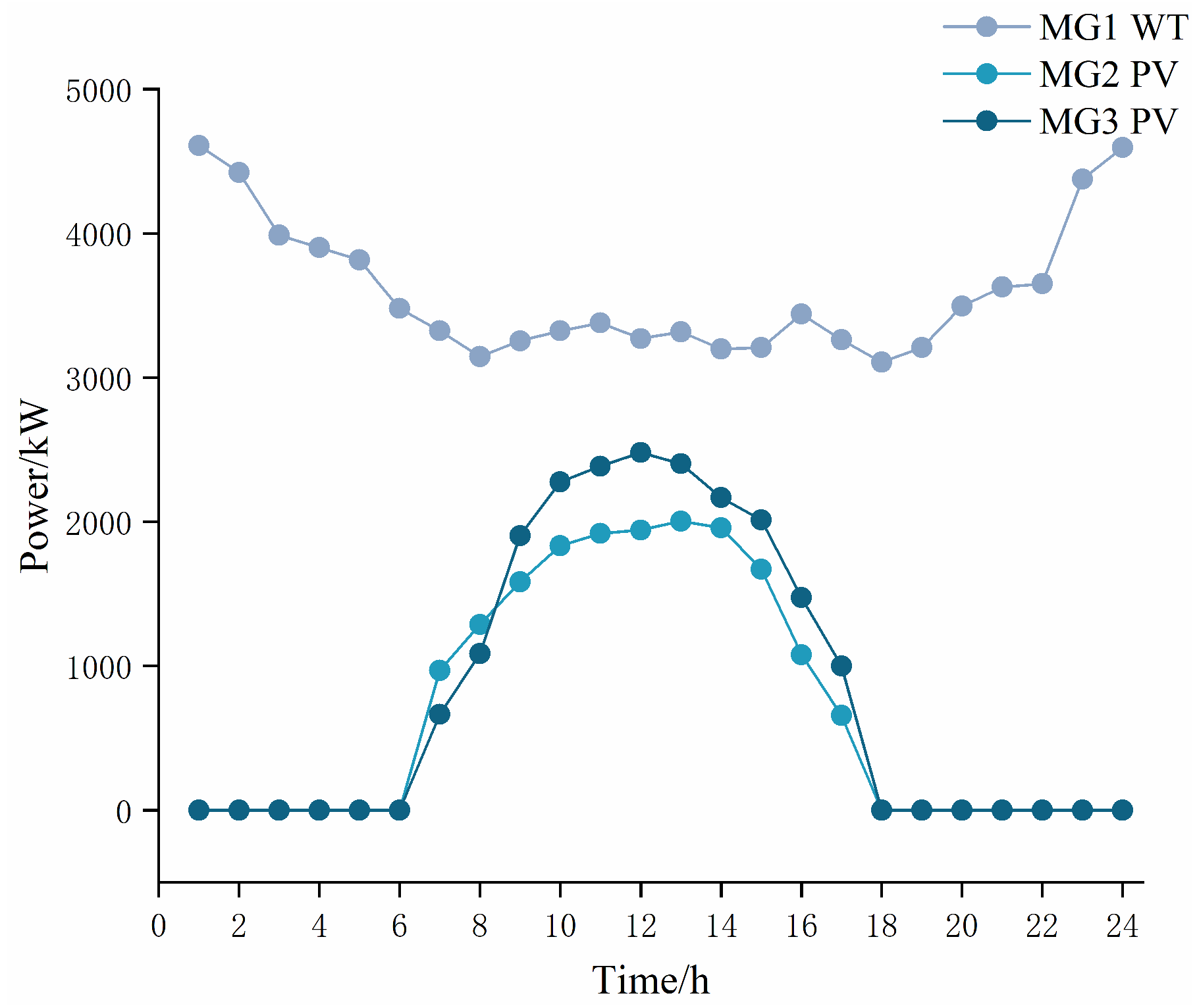
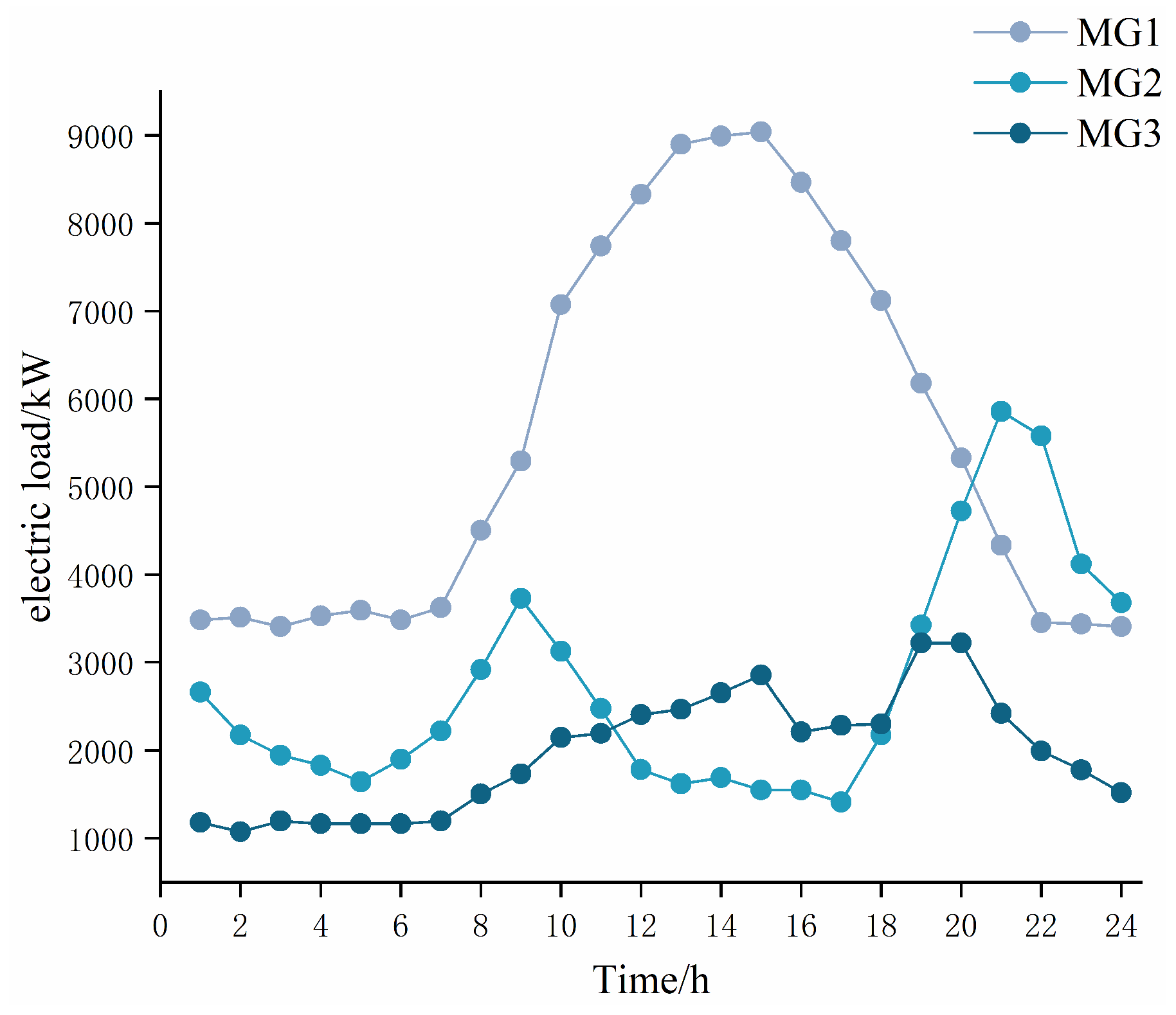
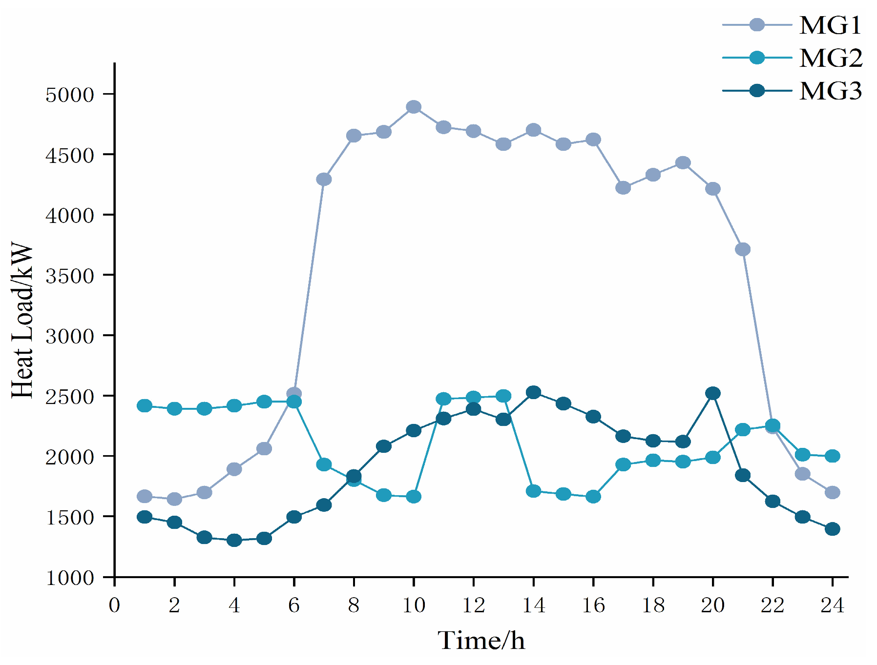
6.1. Basic Data

This paper considers the issue of electricity and hydrogen energy trading between three MGs. The system parameters used in the model are listed in Appendix A,

Table A1. System parameters.

Parameters	Values	Parameters	Values
${\eta }_{CHP}$	0.35	${\eta }_{loss}$	0.01
$Q_{CH4}({\mathrm{MJ}/\mathrm{m}}^3)$	35	$\eta$	0.95
$h_1$	0.15	$E_{\min }^e/\mathrm{kW}$	500
$h_2$	0.2	$E_{\max }^e/\mathrm{kW}$	1800
$h_m$	0.85	$P_{\max }^{cha}/\mathrm{kW}$	500
${\eta }_{GB}$	0.9	$P_{\max }^{dis}/\mathrm{kW}$	600
$P_{\min }^{CCS}/\mathrm{kW}$	0	$a_{c{o}_2}$	0.55
$P_{\max }^{CCS}/\mathrm{kW}$	600	$b_{c{o}_2}$	0.65
$P_{\min }^{P2G}/\mathrm{kW}$	0	$c_{c{o}_2}$	18.20
$P_{\max }^{P2G}/\mathrm{kW}$	300	$a_1(\mathrm{yuan}/\mathrm{kW})$	0.01176
$P_{\min }^{CHP}/\mathrm{kW}$	1200	$a_2(\mathrm{yuan}/\mathrm{kW})$	0.031
$P_{\max }^{CHP}/\mathrm{kW}$	3000	$b_1(\mathrm{yuan}/\mathrm{kW})$	$4\times {10}^{-6}$
$\gamma$	0.55	${\varsigma }_e(\mathrm{yuan}/\mathrm{kW})$	0.01
$\beta$	1.02	$c_{HS}(\mathrm{yuan}/\mathrm{kg})$	0.005
${\eta }_{H_2}$	0.88	$D(kg/\mathrm{kW})$	0.425
${\eta }_{MR}$	0.55	$\epsilon (\mathrm{yuan}/\mathrm{kW})$	0.01
${\sigma }_{HS}$	2%	${\lambda }_e^{cut}(\mathrm{yuan}/\mathrm{kW})$	0.03
${\eta }_{HSC}$	0.93	${\lambda }_e^{tran}(\mathrm{yuan}/\mathrm{kW})$	0.01
${\eta }_{HSD}$	0.93	${\lambda }_r^{cut}(\mathrm{yuan}/\mathrm{kW})$	0.016
$H{S}_{\min }/\mathrm{kg}$	10	$a_e(\mathrm{yuan}/\mathrm{kW})$	0.01
$H{S}_{\max }/\mathrm{kg}$	100	$a_h(\mathrm{yuan}/\mathrm{kg})$	0.95
$H_{\max }^{HSC}/\mathrm{kg}$	50	$P_{ij,\max }^{P2P}/\mathrm{kW}$	2000
$H_{\min }^{HSC}/\mathrm{kg}$	50	$P_{ij,\max }^{H2H}/\mathrm{kg}$	50

[21,43,48,49], and the purchase and sale prices of electricity and natural gas in the external market are shown in Appendix A,

Table A2. Purchase and sale of electricity and natural gas prices.

Parameters	Time Periods	Price/(CNY/(kW·h))
Electricity price	Valley tariff (7–23 h)	0.4
	Parity tariff (8–11 h,15–18 h)	0.75
	Peak tariff (12–14 h,19–22 h)	1.2
Natural gas price	all day	3.5 (CNY/m3)

[50]. This study assumes that the fluctuation deviation of PV and WT generator output is 10% of the predicted value and that PV and WT power generation data for each MG are acquired from a region’s normal daily data, as shown in Appendix A, Figure A2 [21]. The electricity and heat load for each MG are shown in Appendix A, Figure A3 and Figure A4, and the hydrogen load is shown in Appendix A, Figure A5 [51,52]. In this subsection, the robust coefficient magnitude of the PV and WT output is taken as ${\Gamma }_{PV}=6,{\Gamma }_{WT}=6$, for example. The algorithm simulation is modeled in the MATLAB R2018a compilation environment using the Yalmip optimization tool and solved based on the Gurobi solver.

6.2. Analysis of the Optimization Results of Electricity–Hydrogen Sharing in MEMG Network

6.2.1. Case Comparison

To verify the effectiveness of the proposed electricity–hydrogen sharing operation strategy for the MEMG network, four cases were established for comparative analysis, considering energy sharing between the MEMG network or separate operations, CHP units containing P2G and a CCS, or conventional CHP units, as shown in

Table 2. Case settings.

Case	Electricity–Hydrogen Sharing	CHP with CCS and P2G
1	×	×
2	√	×
3	×	√
4	√	√

.

The solution result for Case 1 is the NB rupture point in Case 2, and the solution result for Case 3 is the Nash bargaining rupture point in Case 4.

Table 3. Results of MEMG network optimization operation in different cases.

Case	MG	Total Cost/CNY	Carbon Trading Costs/CNY	Carbon Emissions/kg	Abandoned PV and WT Amount/kW
1	1	29,584.93	−17,200.68	104,572.58	4548.68
	2	27,610.40	−3666.99	62,331.50	5048.60
	3	27,997.52	−724.45	54,018.02	2130.23
	MEMG network	85,192.86	−21,592.12	222,315.10	11,727.52
2	1	25,960.35	−18,612.31	104,084.49	0.00
	2	24,972.69	−4012.99	59,663.86	0.00
	3	25,868.55	−917.29	53,321.14	0.00
	MEMG network	76,801.59	−23,542.58	217,069.48	0.00
3	1	11,820.48	−25,174.21	101,602.01	1047.02
	2	24,662.49	−4061.43	60,604.35	4676.87
	3	19,677.32	−1120.45	51,040.85	1804.27
	MEMG network	56,160.30	−30,356.10	213,247.20	7528.16
4	1	5926.34	−25,344.62	100,400.62	0.00
	2	20,990.05	−4679.03	55,937.01	0.00
	3	16,812.68	−1199.29	48,524.99	0.00
	MEMG network	43,821.92	−31,222.94	202,862.62	0.00

displays the costs of each MG in all four cases, together with the carbon emission and renewable energy consumption situations.

(1)

In terms of operating costs, the cost of each MG in Case 2 decreased by 3624.58, 2637.71, and 2128.98 CNY compared to Case 1, with decrease rates of 12.25%, 9.55%, and 7.60%, respectively. The total cost of the MEMG network is reduced by 8931.27 CNY, with a decrease rate of 9.85%. WT and PV power consumption rates increased by 5.26%, 15.95%, and 3.68%, respectively. The cost of each MG in Case 4 is reduced by 5894.14, 3672.44, and 2860.64 CNY, with a decrease rate of 47.86%, 14.89%, and 14.56%, respectively. Compared to Case 3, the total cost of the MEMG network is reduced by 12431.22 CNY, with a decrease rate of 21.97%. WT and PV power consumption rates increased by 1.21%, 15.71%, and 9.09%, respectively. This is because the MEMG network prioritizes the use of renewable energy sources to achieve energy trading. Each MG reduces CHP unit generation, which reduces natural gas and electricity purchasing and reduces the cost, while each MG’s renewable energy consumption rate is significantly improved. It can be seen that the MEMG system played a significant role in promoting the consumption of new energy and reducing operating costs.

(2)

In terms of reducing carbon emissions, compared with Case 1, the carbon emission reduction ratios of each MG in Case 2 are 0.47%, 4.28%, and 3.77%, and the carbon emission reduction ratio of the MEMG network is 8.51%. The carbon trading cost of each MG was reduced by 1411.63, 345.99, and 83.01 CNY, with decrease rates of 8.21%, 9.44%, and 26.62%, respectively. The carbon trading cost of the MEMG network was reduced by 1840.63 CNY, with a decrease rate of 9.03%. Compared with Case 3, the reduction ratio of carbon emissions of each MG in Case 4 is 1.18%, 7.70%, and 4.93%, and the reduction ratio of carbon emissions in the MEMG network is 13.81%. The carbon transaction cost of each MG decreased by 170.41, 617.59, and 78.84 CNY, with decrease rates of 0.68%, 15.21%, and 7.04%, respectively. The MEMG network carbon transaction cost decreased by 866.84 CNY, with a decrease rate of 2.86%. This is due to the energy trading between MGs, which reduces the power generation of the CHP units, thus reducing carbon emissions from fuel combustion. The MEMG system achieves low-carbon operation by dynamically adjusting the operation mode and power allocation of microgrids, prioritizing the use of renewable energy to meet load demand.

(3)

Regarding the economic benefits of CHP with P2G and a CCS, the cost of each MG in Case 3 decreased by 17,764.45, 2947.91, and 8320.20 CNY compared to Case 1, with a decrease rate of 60.05%, 10.68%, and 29.72%, respectively. The consumption rates of WT and PV power increased by 4.05%, 1.25%, and 1.64%, respectively. The cost of each MG in Case 4 is reduced by 20,034.01, 3982.63, and 9055.86 CNY, with decrease rates of 70.17%, 15.95%, and 35.01%, respectively. Compared to Case 2, the WT and PV energy consumption rates are unchanged, because in the case of MG energy sharing, the WT and PV energy consumption rates are 100 percent in all MG. By integrating P2G technology with conventional CHP units, the EL primarily converts surplus PV and WT into hydrogen energy while simultaneously producing natural gas. This natural gas is then fed into the CHP unit to meet electrical and thermal demands, thereby enhancing renewable energy utilization and reducing the system’s dependence on external natural gas and electricity purchases, ultimately lowering operational costs for each microgrid.

(4)

Regarding the low carbon benefits of CHP with P2G and a CCS, compared with Case 1, the reduction ratio of carbon emissions of each MG in Case 3 is 2.84%, 2.77%, and 5.51%, and the reduction ratio of carbon emissions in the MEMG network is 11.12%. The carbon trading cost of each MG decreased by 7973.53, 394.44, and 396.00 CNY, with a rate of decrease of 46.36%, 10.07%, and 26.62%, respectively. The carbon trading cost of the MEMG network was reduced by 8763.97 CNY, with a decrease rate of 40.59%. Compared with Case 2, the reduction ratio of carbon emissions of each MG in Case 4 is 3.54%, 6.25% and 8.99%, and the reduction ratio of carbon emissions in the MEMG network is 18.78%. The carbon trading cost of each MG decreased by 6732.31, 666.04, and 282.00 CNY, with a rate of decrease of 36.17%, 16.60%, and 30.74%, respectively. The carbon trading cost of the MEMG network decreased by 7680.35 CNY, with a decrease rate of 32.62%. The integration of the CCS with conventional CHP systems enables direct sequestration of combustion-generated carbon dioxide, significantly reducing the operational carbon footprint. Furthermore, the P2G unit may generate natural gas using renewable energy, which lowers the amount of natural gas and electricity the system must purchase and can further lower carbon emissions. It shows that the CCS unit and the P2G unit can effectively realize the low-carbon operation of the MEMG network.

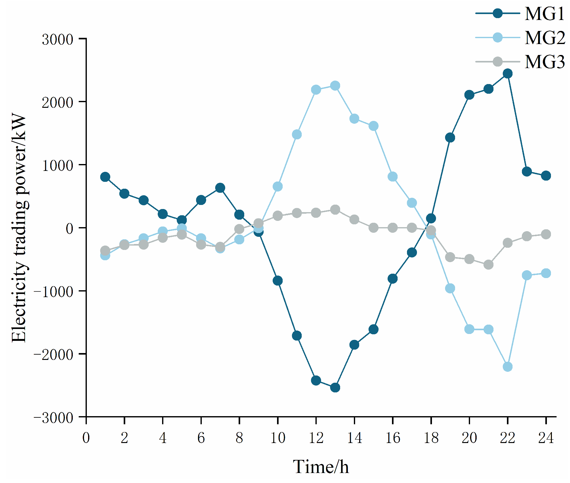
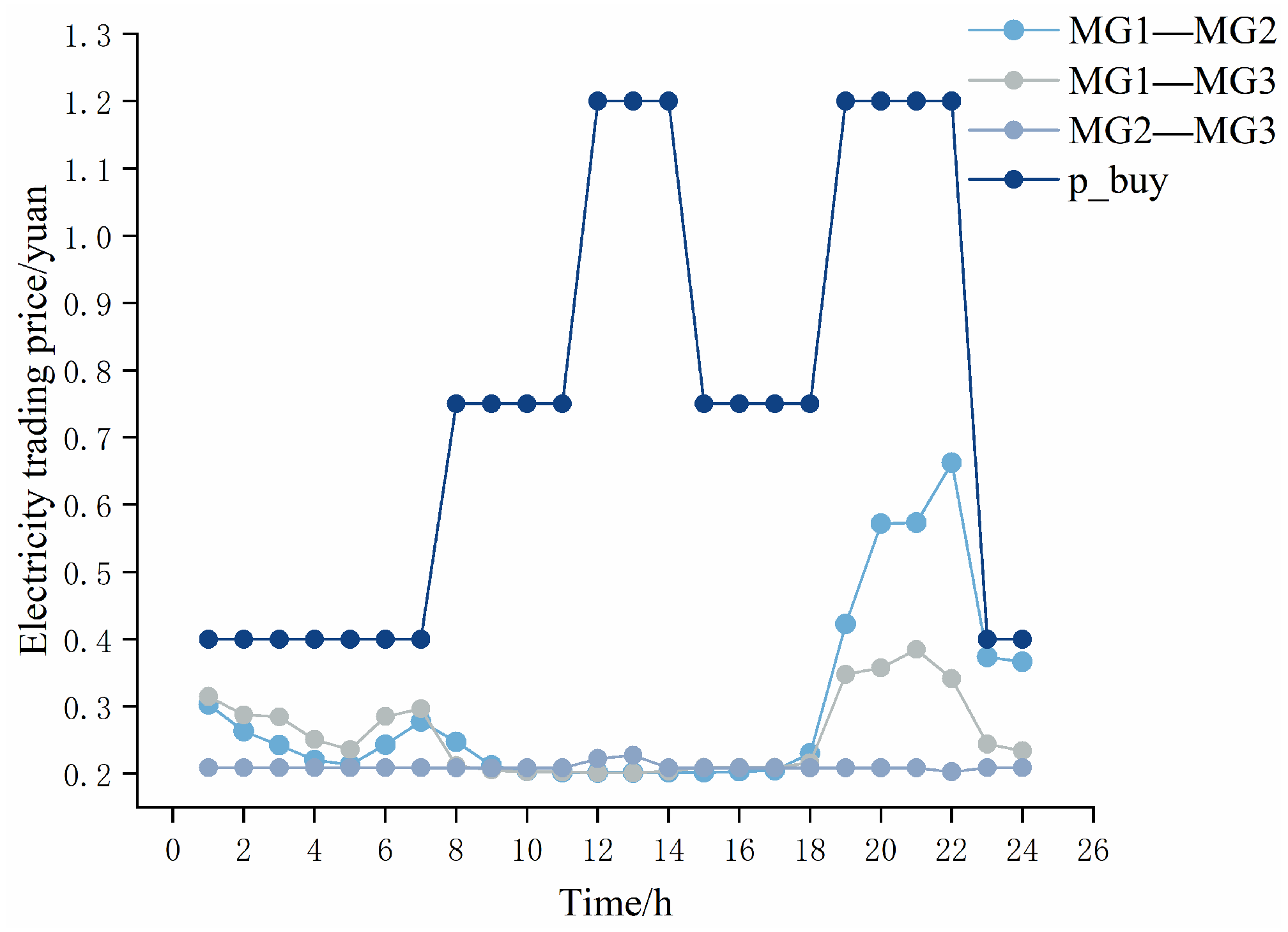
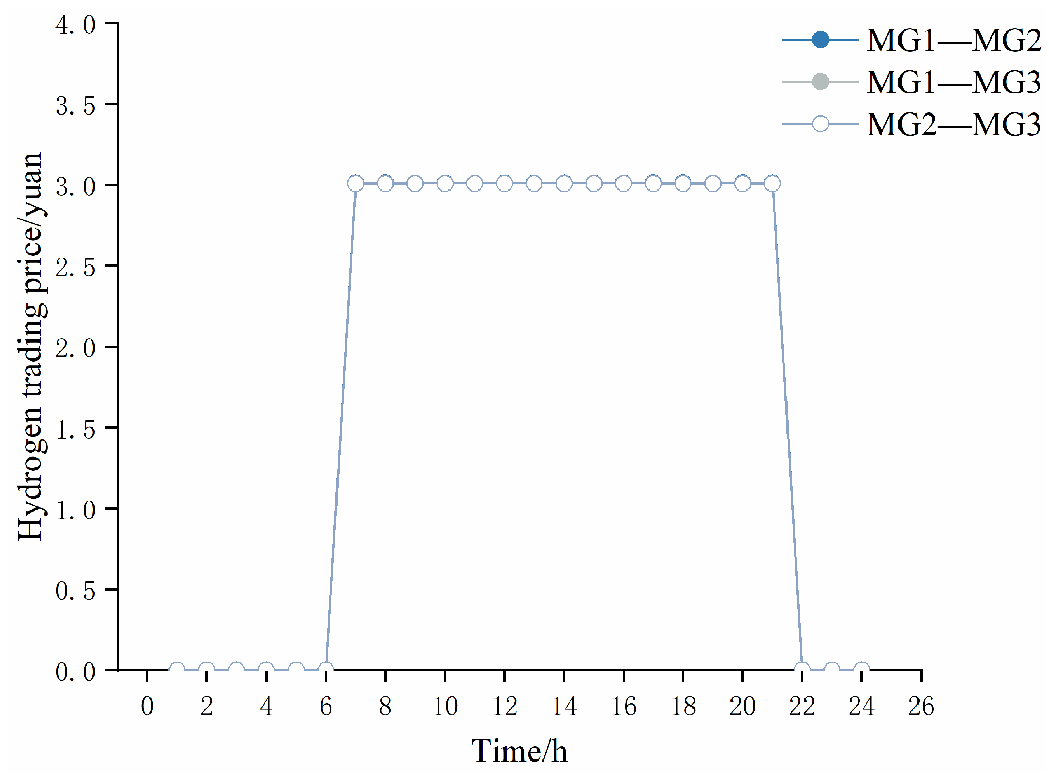
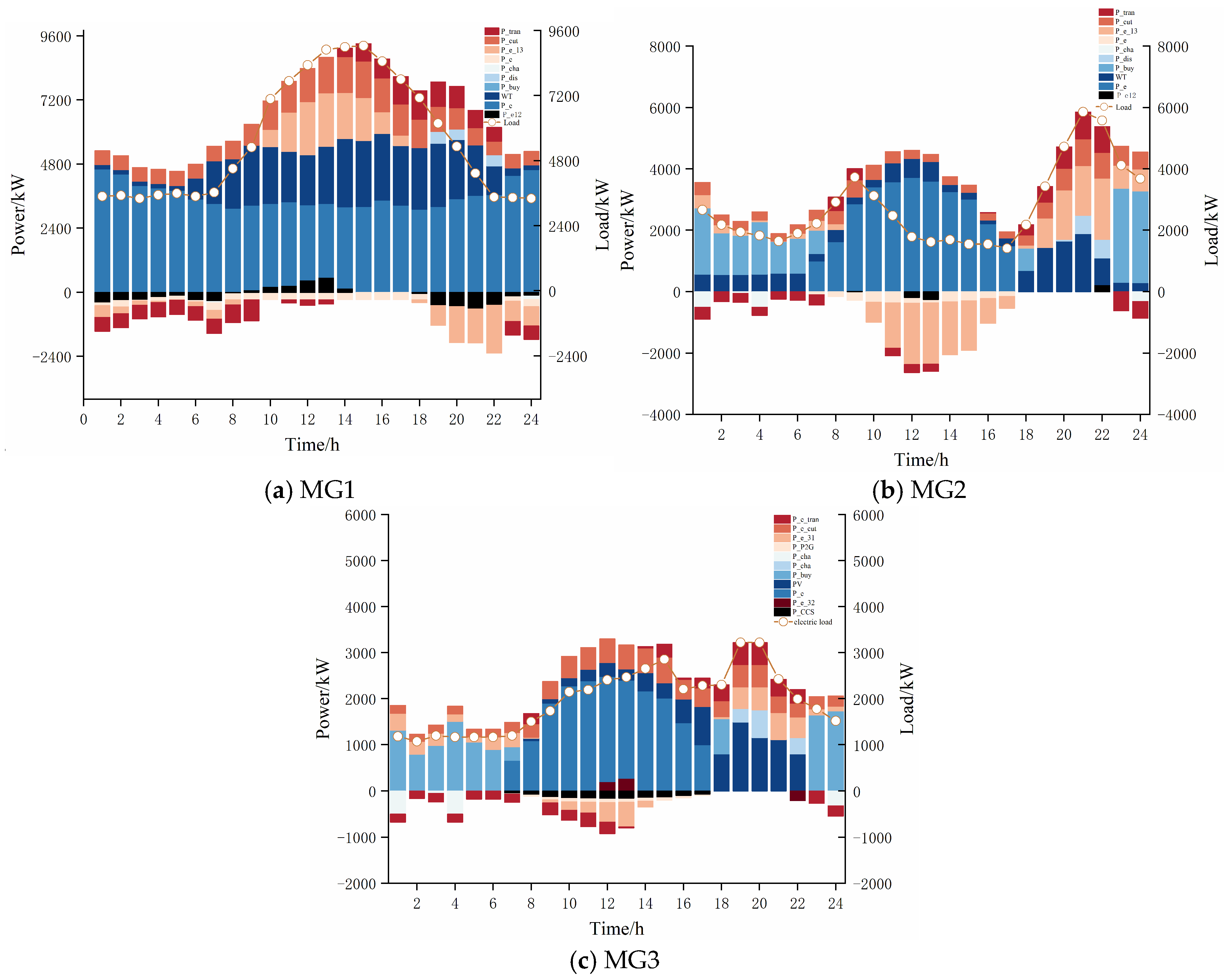
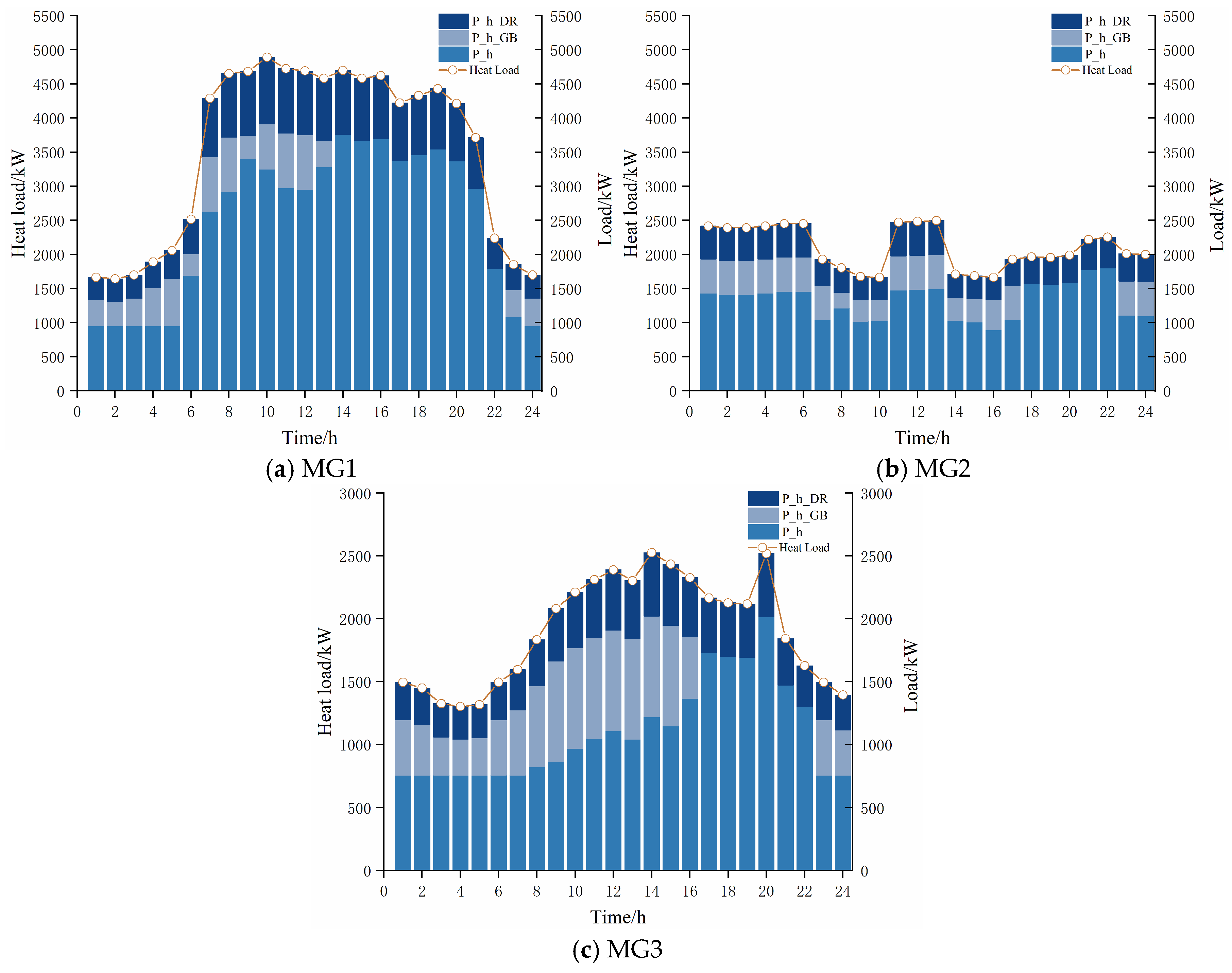
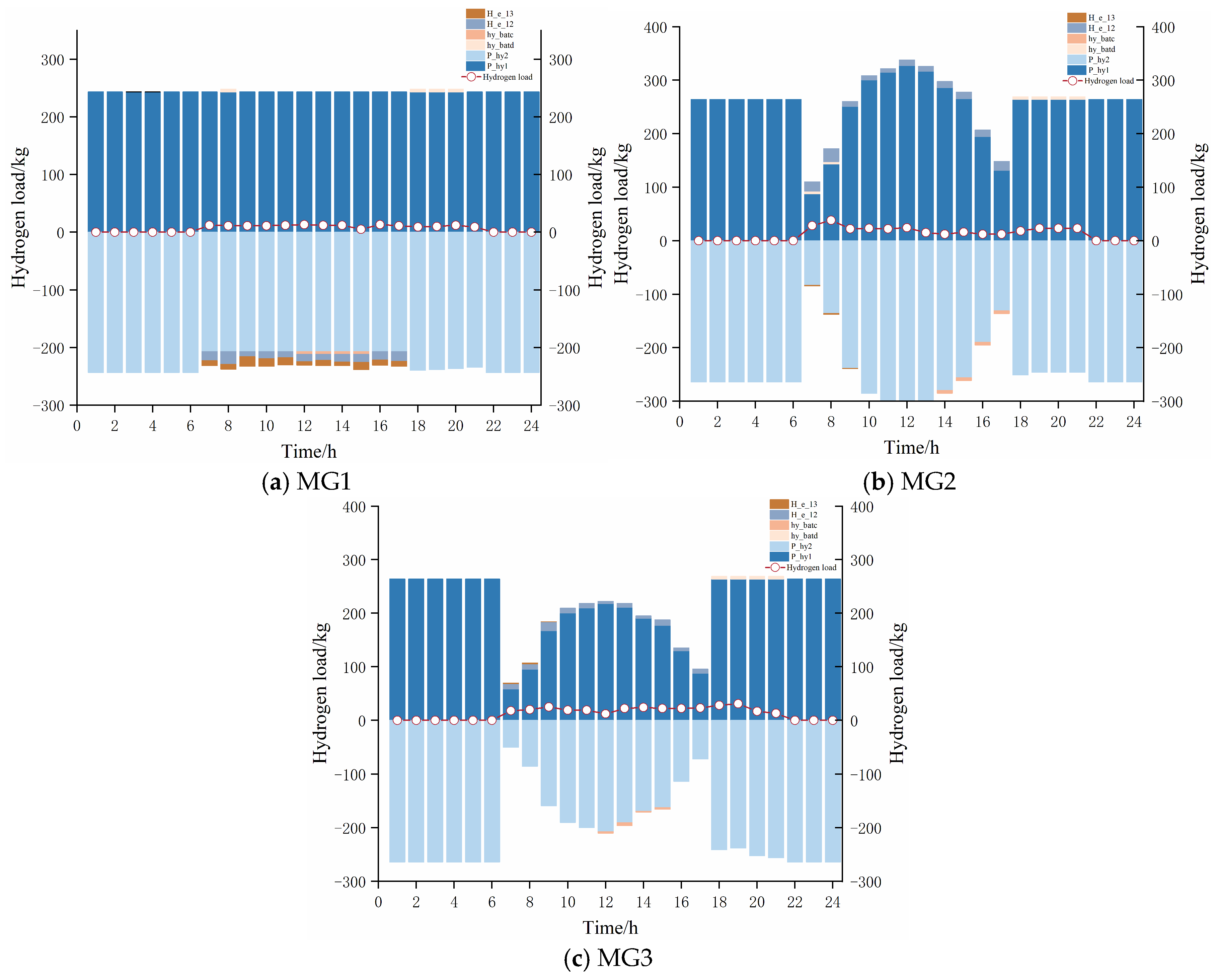
6.2.2. Analysis of the Optimization Results of Electricity–Hydrogen Sharing in MEMG Network

Figure 4 shows the electricity trading results between MGs. It can be seen that there is surplus WT power generation in MG1 between 0–8 h and 18–24 h, so electricity is transported to MG2 and MG3, which are unable to generate electricity at night, resulting in energy shortages. During 9–17 h, MG1 experienced insufficient power supply due to a surge in daytime electricity load, while at this time, the PV power generation of MG2 and MG3 was at its peak, thus transferring excess electricity to MG1. Figure 5 depicts the electricity trading prices between MGs, and each MG’s electricity trading price is within the range of electricity price for purchasing and selling electricity to the DSO. Each MG can sell electricity when there is a surplus at a higher trading price than selling electricity to the DSO, and buy electricity when there is a shortage at a lower trading price than purchasing electricity from the DSO, thereby increasing the MGs’ revenues. It can be seen that in the MEMG system, each MG can meet load demand and reduce operating costs through electricity trading between each other. Figure 6 shows the hydrogen energy trading results between MGs. Due to the low hydrogen load of MG1 and the high output of renewable energy, more hydrogen energy can be created and transmitted to MG2 and MG3 in 8–21 h. Figure 7 shows the price of hydrogen energy trading between MGs. The price of trading hydrogen energy is less than the price of purchasing natural gas.

Figure 8, Figure 9 and Figure 10 show the optimal scheduling results within each MG. In Figure 8, the CHP unit generates power within the power range, and the renewable energy output is higher in 1–8 h and 18–24 h. MG1 chooses to provide electricity to MG2 and MG3; in 10–17 h, MG1 chooses to purchase power from MG2, and in 9–14 h, it chooses to purchase power from MG3, and save costs through the energy transaction between the MGs. Under the time-of-use electricity pricing mechanism, the ESS is mainly charged at 1–4 h, 6–7 h, and 23–24 h and discharged during peak hours of 19–20 h and 22 h. The DR mechanism uses curtailable and transferable loads to adjust the power supply. The heat load is given by CHP, GB, and DR, as shown in Figure 9. As seen in Figure 10, the hydrogen generated by EL is transported to the MR device, held in HES for hydrogen load supply, or transported to other MGs.

6.3. Analysis of Benefit Distribution Results Based on ANB

Table 4. Distribution of model benefits under symmetric NB and ANB.

	MG	Electricity Trading Amount/kW	Hydrogen Trading Amount/kg	Costs Before Participating in Energy Sharing/CNY	Costs After Participating in Energy Sharing/CNY	Bargaining Costs/CNY	Final Allocation Cost/CNY	Increase in Revenue/CNY
ANB	MG1	25,672.80	262.45	11,820.48	10,114.87	4188.52	5926.35	5894.14
	MG2	20,705.69	149.53	24,662.49	18,213.81	−2776.24	20,990.05	3672.44
	MG3	6272.04	89.80	19,677.32	15,500.54	−1312.14	16,812.68	2864.64
Symmetric NB	MG1	25,672.80	262.45	11,820.48	10,114.87	2566.86	7548.01	4272.48
	MG2	20,705.69	149.53	24,662.49	18,213.81	−2274.25	20,488.07	4174.43
	MG3	6272.04	89.80	19,677.32	15,500.54	−149.87	15,650.41	4026.91

compares and analyzes the utility of the ANB method developed in this paper in terms of fair benefit distribution based on Case 4. When the benefits are distributed based on the standard NB method, all the MGs have the same weight, and the benefit enhancement of each MG is equal, which is about 4157.94 CNY. However, when the energy contribution of each MG is different, it is obvious that this method is unfair. When the ANB method proposed in this paper is used, MG1 tends to allocate more benefits due to its large electricity and hydrogen energy trading, which contribute the most to the energy trading process. MG2 and MG3 receive a lower benefit allocation in energy sharing since they trade less electricity and hydrogen. It is shown that the ANB approach described in this study can be used to encourage energy trading among MGs and attain a fair distribution of benefits to them following energy sharing.

6.4. Effectiveness Analysis of Improved ADMM Algorithm

In order to verify the effectiveness of the improved ADMM algorithm, the iteration curves of the conventional ADMM and the improved ADMM algorithm, using MG1 as an example, are displayed in Figure 11 and Figure 12. The iteration curves for MG2 and MG3 are shown in Appendix A, Figure A6 and Figure A7.

The penalty factor for traditional ADMM remains unchanged during the iteration process, with 70 and 22 iterations for Subproblems 1 and 2, respectively, as shown in Figure 11a and Figure 12a. The improved ADMM dynamically corrects the penalty factor based on the quantitative relationship between the original residuals and the pairwise residuals, resulting in a continuous correction of the initial penalty factor during the iteration process, which reduces the randomness of the solution caused by the initial penalty factor. The iteration times for Subproblem 1 and Subproblem 2 are 38 and 14. The computational workload decreased by 45.7% and 36.4%, respectively, as shown in Figure 11b and Figure 12b. Therefore, the improved ADMM algorithm proposed in this paper enhances the efficiency of obtaining the optimal scheduling results for the MG, providing an effective approach for solving distributed optimization problems.

6.5. Result Analysis of Robust Optimization Methods

Table 5. Model costs under robust and deterministic optimization methods.

Method	MG	Costs Before Participating in Energy Sharing/CNY	Bargaining Costs/CNY	Final Costs/CNY
Robust optimization methods	1	11,820.48	4188.52	5926.35
	2	24,662.49	−2776.24	20,990.05
	3	19,677.32	−1312.14	16,812.68
	MEMG network	56,160.30	100.14	43,729.08
Deterministicmethod	1	11,269.23	2687.68	4215.62
	2	21,426.47	−1672.37	16,071.55
	3	16,492.34	−1209.42	12,407.32
	MEMG network	49,188.04	−194.12	32,694.49

presents a cost comparison between the deterministic and robust optimization approaches. This comparison aims to confirm the efficacy of the robust optimization method in managing the uncertainty of WT and PV production. The system must increase the output of the purchased power and the natural gas-sourced CHP units in order to achieve the power balance because the robust optimization method accounts for the fluctuation in the system’s renewable energy output, which leads to an increase in the cost of the MEMG network. Nonetheless, compared to deterministic methods that ignore fluctuations in WT and PV output, the results of robust optimization methods are more realistic.

6.6. Analysis of the Results of Different Scheduling Methods

From

Table 6. Results of different scheduling methods.

Scheduling Method	MG	Total Cost/CNY
Centralized scheduling	1	29,584.93
	2	27,610.40
	3	27,997.52
	MEMG network	85,192.86
Distributed scheduling	1	25,960.35
	2	24,972.69
	3	25,868.55
	MEMG network	76,801.59

, it can be seen that the cost of distributed optimization scheduling is 2.5% higher than that of centralized optimization scheduling, and the solution obtained from distributed optimization is very close to the global optimal solution obtained from centralized optimization scheduling. The reason why this study did not choose a centralized optimization scheduling method is because all information from the microenergy network needs to be transmitted to the central energy manager for processing and decision-making, which may lead to excessive load on the communication network and increase the risk of system collapse. In addition, if a microenergy network experiences a connection failure and operates in islanding mode, it cannot receive energy support from other microenergy networks. At this time, a single microenergy network must achieve energy self-sufficiency, which may have certain shortcomings in operational stability.

7. Conclusions

In this paper, we propose a low-carbon optimal operation strategy for electricity–hydrogen sharing in an MEMG network based on ANB and decompose it into two continuous subproblems: minimizing the operation cost of the MEMG network and maximizing payment benefits. The improved ADMM algorithm is used for distributed solutions. The following conclusions can be drawn from the several case studies:

(1)

The suggested MEMG electricity–hydrogen sharing model, which is based on ANB, mitigates carbon emissions, increases each MG’s economy, and saves the overall cost of the MEMG network compared to MG’s independent operation. Specifically, the cost of each MG decreased by 5894.14, 3672.44, and 2806.64 CNY, respectively, while the total cost of the MEMG network decreased by 12,431.22 CNY. The electricity consumption of WT and PV power generation increased by 1.21%, 15.71%, and 9.09%, respectively, with a reduction rate of 1.18%, 8%, and 9.25% in carbon emissions.

(2)

Low-carbon operation of the system was achieved with the addition of P2G and a CCS to the conventional CHP units. Specifically, the carbon emission reduction ratios were 2.84%, 2.77%, and 5.51% for each MG and 11.12% for the MEMG network.

(3)

Compared with the benefit distribution mechanism based on symmetric Nash bargaining, this study proposes an ANB profit distribution model that takes the contribution of each MG as the bargaining power, which can achieve a fair distribution of benefits after electricity–hydrogen sharing and effectively stimulate the enthusiasm of each MG to participate in energy trading.

(4)

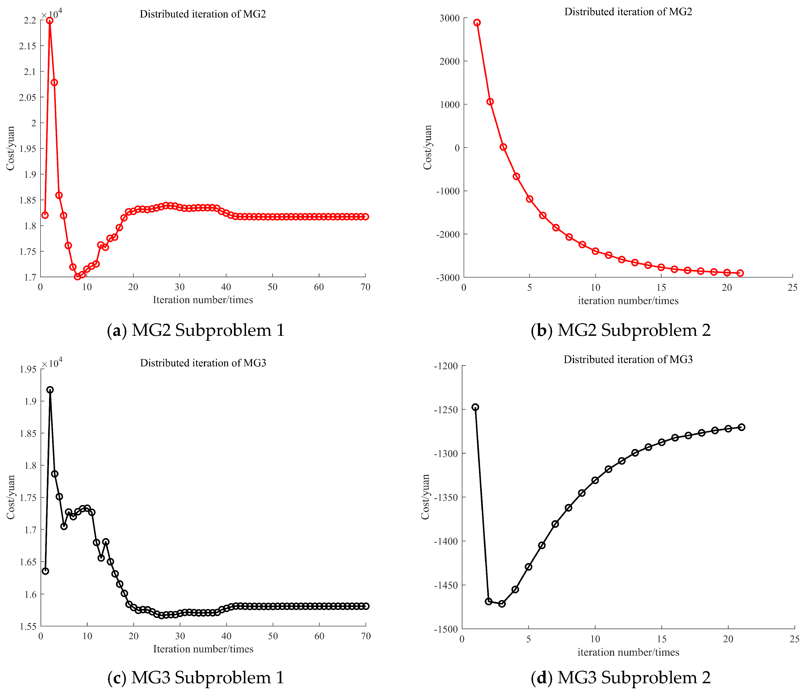
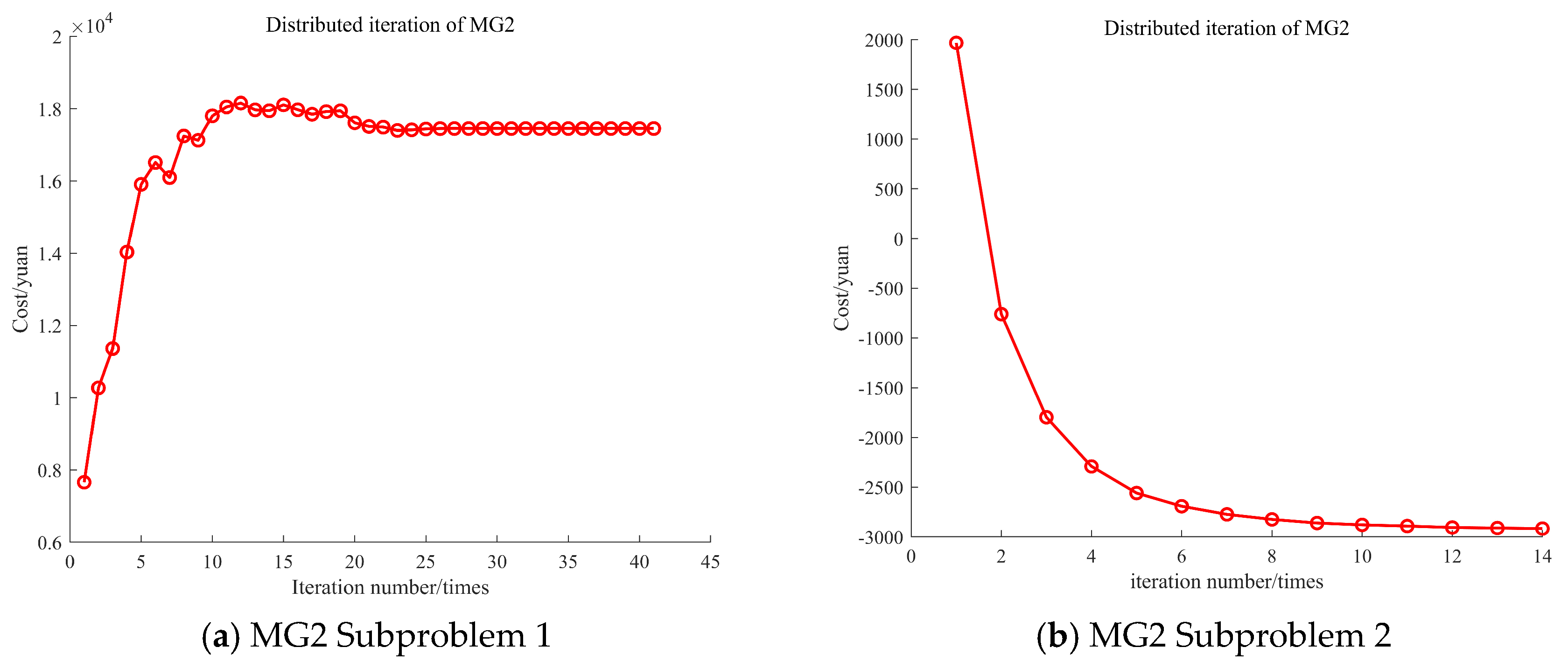
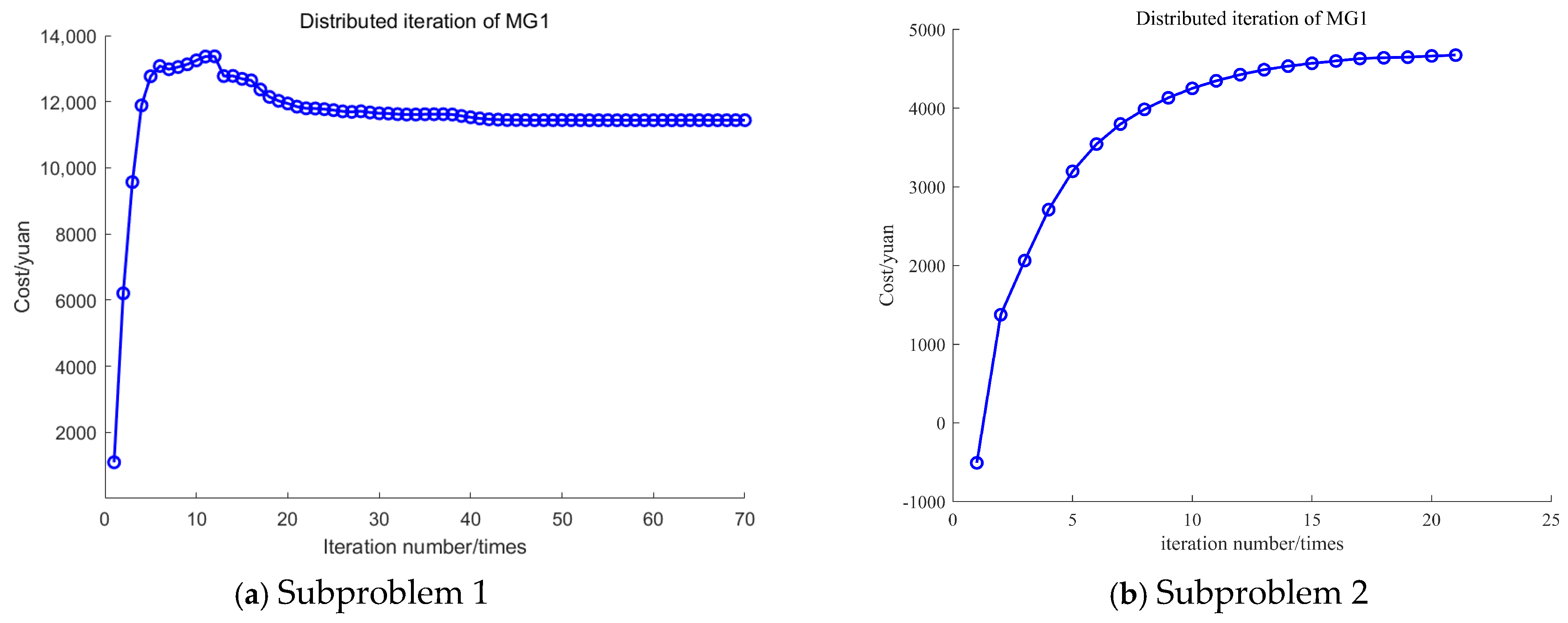
The improved ADMM approach has strong convergence because it dynamically adjusts the penalty factor in accordance with the quantitative relationship between the paired residuals and the original residuals. Compared with the traditional ADMM algorithm, the number of iterations is reduced by nearly 40%; therefore, the improved ADMM algorithm achieves an efficient solution to the MEMG network operation problem while protecting the privacy of each MG.

This study only considers the interaction between electric energy and hydrogen energy, and cannot further unleash the flexibility of MEMG systems. Future research can include shared energy storage systems, intelligent transportation systems, etc., in the MEMG network for discussion. In addition, in terms of system uncertainty, this study only considers the uncertainty of renewable energy output. In the future, load uncertainty can be included in the research, and distributed robust optimization with stronger applicability can be used to manage uncertainty problems.

References

- Fang, X.; Dong, W.; Wang, Y.; Yang, Q. Multiple time-scale energy management strategy for a hydrogen-based multi-energy microgrid. Appl. Energy 2022, 328, 120195. [Google Scholar] [CrossRef]
- Qian, K.; Lv, T.; Yuan, Y. Integrated Energy System Planning Optimization Method and Case Analysis Based on Multiple Factors and A Three-Level Process. Sustainability 2021, 13, 7425. [Google Scholar] [CrossRef]
- Wang, M.; Shi, Z.; Luo, W.; Sui, Y.; Wu, D. Distributionally robust optimal scheduling of integrated energy systems including hydrogen fuel cells considering uncertainties. Energy Rep. 2023, 10, 1575–1588. [Google Scholar] [CrossRef]
- Karimi, H.; Jadid, S. A collaborative hierarchal optimization framework for sustainable multi-microgrid systems considering generation and demand-side flexibilities. Sustain. Energy Grids Networks 2023, 35, 101087. [Google Scholar] [CrossRef]
- Zhang, G.; Niu, Y.; Xie, T.; Zhang, K. Multi-level distributed demand response study for a multi-park integrated energy system. Energy Rep. 2023, 9, 2676–2689. [Google Scholar] [CrossRef]
- Wang, K.; Liang, Y.; Jia, R.; Wu, X.; Wang, X.; Dang, P. Two-stage stochastic optimal scheduling for multi-microgrid networks with natural gas blending with hydrogen and low carbon incentive under uncertain envinronments. J. Energy Storage 2023, 72, 108319. [Google Scholar] [CrossRef]
- Cui, Y.; Xu, Y.; Wang, Y.; Zhao, Y.; Zhu, H.; Cheng, D. Peer-to-peer energy trading with energy trading consistency in interconnected multi-energy microgrids: A multi-agent deep reinforcement learning approach. Int. J. Electr. Power Energy Syst. 2024, 156, 109753. [Google Scholar] [CrossRef]
- Zhang, K.; Gao, C.; Zhang, G.; Xie, T.; Li, H. Electricity and heat sharing strategy of regional comprehensive energy multi-microgrid based on double-layer game. Energy 2024, 293, 130655. [Google Scholar] [CrossRef]
- Ruan, H.; Gao, H.; Qiu, H.; Gooi, H.B.; Liu, J. Distributed operation optimization of active distribution network with P2P electricity trading in blockchain environment. Appl. Energy 2023, 331, 120405. [Google Scholar] [CrossRef]
- Esfahani, M.M. A hierarchical blockchain-based electricity market framework for energy transactions in a security-constrained cluster of microgrids. Int. J. Electr. Power Energy Syst. 2022, 139, 108011. [Google Scholar] [CrossRef]
- Hamouda, M.R.; Nassar, M.E.; Salama, M. Blockchain-based sequential market-clearing platform for enabling energy trading in Interconnected Microgrids. Int. J. Electr. Power Energy Syst. 2023, 144, 108550. [Google Scholar] [CrossRef]
- Xu, Z.; Wang, Y.; Dong, R.; Li, W. Research on multi-microgrid power transaction process based on blockchain Technology. Electr. Power Syst. Res. 2022, 213, 108649. [Google Scholar] [CrossRef]
- Yan, W.; Liu, J. Optimization Strategy for Master-slave Game Operation in Multi-microgridMarket Based on Deep Learning. Proc. CSU-EPSA 2022, 34, 120–128. [Google Scholar] [CrossRef]
- Wu, Q.; Xie, Z.; Li, Q.; Ren, H.; Yang, Y. Economic optimization method of multi-stakeholder in a multi-microgrid system based on Stackelberg game theory. Energy Rep. 2022, 8, 345–351. [Google Scholar] [CrossRef]
- Li, Y.; Zhang, X.; Wang, Y.; Qiao, X.; Jiao, S.; Cao, Y.; Xu, Y.; Shahidehpour, M.; Shan, Z. Carbon-oriented optimal operation strategy based on Stackelberg game for multiple integrated energy microgrids. Electr. Power Syst. Res. 2023, 224, 109778. [Google Scholar] [CrossRef]
- Du, J.; Han, X.; Wang, J. Distributed cooperation optimization of multi-microgrids under grid tariff uncertainty: A nash bargaining game approach with cheating behaviors. Int. J. Electr. Power Energy Syst. 2024, 155, 109644. [Google Scholar] [CrossRef]
- Xu, J.; Yi, Y. Multi-microgrid low-carbon economy operation strategy considering both source and load uncertainty: A Nash bargaining approach. Energy 2022, 263, 125712. [Google Scholar] [CrossRef]
- Duan, P.; Zhao, B.; Zhang, X.; Fen, M. A day-ahead optimal operation strategy for integrated energy systems in multi-public buildings based on cooperative game. Energy 2023, 275, 127395. [Google Scholar] [CrossRef]
- Jun, Z.; Min, Z.; Zhang, S.; Qi, Y. Optimization Strategy for Cooperative Operation of Multiple Microgrids Considering Carbon Trading and New Energy Uncertainty. Electr. Power 2023, 56, 62–71. [Google Scholar]
- Chen, Y.; Pei, W.; Ma, T.; Xiao, H. Asymmetric Nash bargaining model for peer-to-peer energy transactions combined with shared energy storage. Energy 2023, 278, 127980. [Google Scholar] [CrossRef]
- Wu, J.; Lou, P.; Guang, M.; Huang, Y.; Zhang, Y. Operation Optimization Strategy of Multi-microgrids Energy Sharing Based on Asymmetric Nash Bargaining. Power Syst. Technol. 2022, 46, 2711–2723. [Google Scholar]
- Ding, J.; Gao, C.; Song, M.; Yan, X.; Chen, T. Optimal operation of multi-agent electricity-heat-hydrogen sharing in integrated energy system based on Nash bargaining. Int. J. Electr. Power Energy Syst. 2023, 148, 108930. [Google Scholar] [CrossRef]
- Li, Z.; Wu, L.; Xu, Y.; Wang, L.; Yang, N. Distributed tri-layer risk-averse stochastic game approach for energy trading among multi-energy microgrids. Appl. Energy 2022, 331, 120282. [Google Scholar] [CrossRef]
- Shuai, X.; Wang, X.; Wu, X.; Wang, Y.; Song, Z.; Wang, B.; Ma, Z. Peer-to-peer multi-energy distributed trading for interconnected microgrids: A general Nash bargaining approach. Int. J. Electr. Power Energy Syst. 2022, 138, 107892. [Google Scholar] [CrossRef]
- Cui, M.; Xuan, M.; Lu, Z.; He, L. Operation Optimization Strategy of Multi Integrated Energy Service Companies Based on Cooperative Game Theory. Proc. CSEE 2022, 42, 3548–3564. [Google Scholar] [CrossRef]
- Luo, P.; Zhou, H.; Xu, L.; Lv, Q.; Wu, Q. Day-ahead Optimal Scheduling of Multi-microgrids with Combined Cooling. Heat. Power Based Interval Optimization. Autom. Electr. Power Syst. 2022, 46, 137–146. [Google Scholar]
- Zheng, W.; Lu, H.; Zhu, J. Incentivizing cooperative electricity-heat operation: A distributed asymmetric Nash bargaining mechanism. Energy 2023, 280, 128041. [Google Scholar] [CrossRef]
- Gao, H.; Cai, W.; He, S.; Jiang, J.; Liu, J. Multi-energy sharing optimization for a building cluster towards net-zero energy system. Appl. Energy 2023, 350, 121778. [Google Scholar] [CrossRef]
- Ding, L.; Cui, Y.; Yan, G.; Huang, Y.; Fan, Z. Distributed energy management of multi-area integrated energy system based on multi-agent deep reinforcement learning. Int. J. Electr. Power Energy Syst. 2024, 157, 109867. [Google Scholar] [CrossRef]
- Dong, L.; Yang, Z.; Qiao, Y.; Cheng, S.; Wang, X.; Pu, T. Optimization and scheduling of integrated energy multi microgrid systems based on hierarchical constraint reinforcement learning. J. Electr. Eng. Technol. 2024, 39, 1436–1453. [Google Scholar] [CrossRef]
- Shen, R.; Zheng, R.; Yang, D.; Zhao, J. Two-layer energy dispatching and collaborative optimization of regional integrated energy system considering stakeholders game and flexible load management. Energy Convers. Manag. 2025, 329, 119656. [Google Scholar] [CrossRef]
- Zhong, J.; Cao, Y.; Li, Y.; Tan, Y.; Peng, Y.; Cao, L.; Zeng, Z. Distributed modeling considering uncertainties for robust operation of integrated energy system. Energy 2021, 224, 120179. [Google Scholar] [CrossRef]
- Li, S.; Zhang, L.; Liu, X.; Zhu, C. Collaborative operation optimization and benefit-sharing strategy of rural hybrid renewable energy systems based on a circular economy: A Nash bargaining model. Energy Convers. Manag. 2023, 283, 116918. [Google Scholar] [CrossRef]
- Zhang, Z.; Wang, Y.; Wang, C.; Su, Y.; Wang, Y.; Dai, Y.; Cui, C.; Zhang, W. Distributed Chance-Constrained Optimal Dispatch for Integrated Energy System with Electro-Thermal Couple and Wind-Storage Coordination. IEEE Trans. Ind. Appl. 2024, 61, 833–846. [Google Scholar] [CrossRef]
- Tan, J.; Wu, Q.; Wei, W.; Liu, F.; Li, C.; Zhou, B. Decentralized robust energy and reserve Co-optimization for multiple integrated electricity and heating systems. Energy 2020, 205, 118040. [Google Scholar] [CrossRef]
- Qin, G.; Yan, Q.; Kammen, D.M.; Shi, C.; Xu, C. Robust optimal dispatching of integrated electricity and gas system considering refined power-to-gas model under the dual carbon target. J. Clean. Prod. 2022, 371, 133451. [Google Scholar] [CrossRef]
- Song, X.; Li, W.; Zhou, J.; Liu, X.; Sun, Y. Low-carbon economic dispatch considering P2G and load flexibility characteristic under carbon trading mechanism. Electr. Meas. Instrum. 2022, 423, 138812. [Google Scholar]
- Lan, L.; Zhang, Y.; Zhang, X.; Zhang, X. Price effect of multi-energy system with CCS and P2G and its impact on carbon-gas-electricity sectors. Appl. Energy 2024, 359, 122713. [Google Scholar] [CrossRef]
- Wu, Q.; Li, C. Modeling and operation optimization of hydrogen-based integrated energy system with refined power-to-gas and carbon-capture-storage technologies under carbon trading. Energy 2023, 270, 126832. [Google Scholar] [CrossRef]
- Liu, H.; Ma, L.; Wang, Z.; Liu, Y.; Alsaadi, F.E. An overview of stability analysis and state estimation for memristive neural networks. Neurocomputing 2020, 391, 1–12. [Google Scholar] [CrossRef]
- Chen, Y.; Lu, X.; Zhang, H.; Zhao, C.; Xu, Y. Optimal configuration of integrated energy station using adaptive operation mode of combined heat and power units. Int. J. Electr. Power Energy Syst. 2023, 152, 109171. [Google Scholar] [CrossRef]
- Wu, Q.; Xie, Z.; Ren, H.; Li, Q.; Yang, Y. Optimal trading strategies for multi-energy microgrid cluster considering demand response under different trading modes: A comparison study. Energy 2022, 254, 124448. [Google Scholar] [CrossRef]
- Cui, Y.; Yan, S.; Zhong, Z.; Wang, Z.; Zhang, P.; Zhao, Y. Optimal Thermoelectric Dispatching of Regional Integrated Energy System with Power-to-gas. Power Syst. Technol. 2020, 44, 4254–4264. [Google Scholar] [CrossRef]
- Ma, Y.; Wang, H.; Hong, F.; Yang, J.; Chen, Z.; Cui, H.; Feng, J. Modeling and optimization of combined heat and power with power-to-gas and carbon capture system in integrated energy system. Energy 2021, 236, 121392. [Google Scholar] [CrossRef]
- Wu, Q.; Li, C. Economy-environment-energy benefit analysis for green hydrogen based integrated energy system operation under carbon trading with a robust optimization model. J. Energy Storage 2022, 55, 105560. [Google Scholar] [CrossRef]
- Ma, T.; Pei, W.; Xiao, H.; Li, D.; Lv, X.; Hou, K. Cooperative Operation Method for Wind-solar-hydrogen Multi-agent Energy System Based on Nash Bargaining Theory. Proc. CSEE 2021, 41, 25–39. [Google Scholar] [CrossRef]
- Cui, S.; Wang, Y.-W.; Liu, X.-K.; Wang, Z.; Xiao, J.-W. Economic Storage Sharing Framework: Asymmetric Bargaining-Based Energy Cooperation. IEEE Trans. Ind. Inform. 2021, 17, 7489–7500. [Google Scholar] [CrossRef]
- Luo, Z.; Wang, Q.; Wang, H.; Zhao, W.; Yang, L.; Sheng, X. Optimal scheduling of comprehensive energy systems considering carbon capture and electricity to gas conversion. Electr. Power Autom. Equip. 2023, 42, 127–134. [Google Scholar] [CrossRef]
- Zhang, Q.S.; Huang, X.S. Analysis of domestic and foreign hydrogen energy industrial policies andtechnical economy. Low-Carbon Chem. Chem. Eng. 2023, 48, 133–139. [Google Scholar]
- Zhang, D.; Yun, Y.; Wang, X.; He, J.; Dong, H. Economic Dispatch of Integrated Electricity-Heat-Gas Energy SystemConsidering Generalized Energy Storage and Concentrating Solar Power Plant. Autom. Electr. Power Syst. 2021, 45, 33–42. [Google Scholar]
- Jiu, G.; Chenlei, W.; Da, X. Research on optimal operation of electricity-hydrogen integrated station inelectricity market environment. J. Electr. Power Sci. Technol. 2022, 37, 130–139. [Google Scholar] [CrossRef]
- Wu, X.; Li, H.; Wang, X.; Zhao, W. Cooperative Operation for Wind Turbines and Hydrogen Fueling Stations with On-Site Hydrogen Production. IEEE Trans. Sustain. Energy 2020, 11, 2775–2789. [Google Scholar] [CrossRef]