Dependency and Risk Spillover of China’s Industrial Structure Under the Environmental, Social, and Governance Sustainable Development Framework

Abstract

With the growing global emphasis on sustainable development goals, Environmental, Social, and Governance (ESG) factors have emerged as critical considerations in shaping economic policies and strategies. This study employs the ARMA-eGARCH-skewed t and Vine Copula models, combined with the CoVaR method, to investigate the dependence structure and risk spillover pathways across various industrial sectors in China within the ESG framework. By modeling the complex interdependencies among sectors, this research uncovers the relationships between individual industries and the ESG benchmark index, while also analyzing the correlations across different sectors. Furthermore, this study quantifies the risk contagion effects across distinct industries under extreme market conditions and maps the pathways of risk spillovers. The findings highlight the pivotal role of ESG considerations in shaping industrial structures. Empirical results demonstrate that industries such as agriculture, energy, and manufacturing exhibit significant systemic risk characteristics in response to ESG fluctuations. Specifically, the identified risk spillover pathway follows the sequence: agriculture → consumption → ESG → manufacturing → energy. The CoVaR values for agriculture, energy, and manufacturing indicate a significant potential for risk contagion. Moreover, sectors such as real estate, finance, and information technology exhibit significant risk spillover effects. These findings offer valuable empirical evidence and a theoretical foundation for formulating ESG-related policies. This study suggests that effective risk management, promoting green finance, encouraging technological innovation, and optimizing industrial structures can significantly mitigate systemic risks. These measures can contribute to maintaining industrial stability and fostering sustainable economic development.

1. Introduction

Sustainable development has emerged as a critical global priority to address urgent challenges such as environmental degradation, social inequality, and economic instability. The Environmental, Social, and Governance (ESG) framework has become a transformative approach that integrates environmental stewardship, social responsibility, and governance excellence into decision-making processes to enhance resilience and create long-term value [1]. The global adoption of ESG principles is accelerating, aiming to drive green transitions, foster sustainable industrial structures, and align economic growth with environmental and social objectives [2]. As the world’s second-largest economy, China plays a pivotal role in global sustainable development efforts. However, China’s transition from rapid expansion to high-quality development presents unique challenges, characterized by the coexistence of resource-intensive industries and emerging green sectors [3]. High-carbon industries, such as steel, coal, and petrochemicals, still occupy a significant share of the industrial landscape, placing considerable pressure on structural upgrading [4]. Moreover, critical technological breakthroughs in high-end manufacturing, green technologies, and intelligent transformation are still needed. Gaps remain in industrial support mechanisms, the establishment of comprehensive green standards, and the precision of financial support targeted at sustainability objectives [5].

Against this backdrop, the ESG framework is increasingly recognized as a key lever for optimizing China’s industrial structure. By embedding environmental and social considerations into industrial policies and investment decisions, ESG promotes the phasing out of high-carbon sectors, encourages green innovation, and facilitates the transformation toward cleaner, more resilient, and interconnected industries. ESG-driven reforms reshape not only the internal dynamics of individual industries but also the interdependencies among them, influencing resource allocation, production networks, and systemic risk exposures [6].

While a growing body of literature examines the impact of ESG adoption on corporate performance and capital markets, relatively little research focuses on how ESG-driven transitions influence the macro-level industrial structure, the evolving patterns of industrial dependence, and systemic risk spillovers, particularly in the Chinese context. The simultaneous presence of resource-intensive and green industries creates a complex web of interactions that traditional models often fail to adequately capture. Thus, there is a pressing need for more sophisticated, dynamic analyses to understand how ESG transformations reconfigure industrial linkages and risk transmission pathways.

Understanding the evolving dependence structures and risk spillover pathways among industries under the ESG transition is therefore critical. Traditional models, which assume linear and stable relationships, are insufficient to capture the complexity of these dynamic interactions, particularly under extreme economic or environmental shocks. Advanced methods such as Vine Copula models allow for a more flexible, nonlinear, and tail-dependent analysis of industrial interconnections. Meanwhile, the use of Conditional Value at Risk (CoVaR) techniques enables a deeper understanding of systemic risk transmission under ESG-induced transformations.

This study makes a unique contribution by employing dynamic Vine Copula models combined with CoVaR measures to systematically investigate how ESG-driven policies reshape industrial dependence structures and risk spillover mechanisms in China. By capturing the nonlinear, asymmetric, and time-varying characteristics of industry linkages, our analysis provides novel insights into the hidden systemic risks and resilience pathways emerging from China’s sustainable development agenda. This research not only advances theoretical understanding of industrial dynamics under ESG reforms but also offers important practical implications for policymakers, investors, and industry leaders seeking to optimize resource allocation, enhance industrial resilience, and navigate the complexities of the green transition. This paper is structured as follows. Section 1 introduces the study. Section 2 presents the literature review. Section 3 outlines the research domain and methodology. Section 4 presents the results. Section 5 discusses the main findings and their implications. Finally, Section 6 concludes the paper and offers policy recommendations.

2. Literature Review

ESG has a profound impact on the optimization of industrial structure. Strict environmental regulations, green finance initiatives, and coordinated development strategies have promoted green transformation and reshaped the global value chain.

At the macroeconomic level, ESG frameworks are increasingly recognized as catalysts for sustainable development and industrial restructuring [7]. Studies have shown that ESG-oriented policies, including green finance, carbon pricing, and sustainability disclosure requirements, contribute to the reallocation of resources, decarbonization, and the emergence of high-value, low-emission sectors (Kotsantonis and Serafeim, 2019) [8]. Scholtens (2017) emphasizes how financial systems are progressively aligning with long-term ecological goals [9], while Cruz (2019) and Wei (2024) demonstrate that ESG-linked fiscal tools can enhance macroeconomic resilience and productivity in volatile environments [10,11]. ESG practices have also reshaped supply chain configurations, with green procurement and responsible sourcing mechanisms altering upstream–downstream interdependencies across industries (Wang et al., 2025) [12].

At the micro level, firms with superior ESG performance are found to enjoy better access to capital, lower financing costs, and improved stakeholder trust (Fourgon, 2024; Lins et al., 2017; Kramer and Porter, 2011) [13,14,15]. In the context of emerging markets, Liu (2024) provides compelling evidence from the Chinese bond market, showing that firms with higher ESG ratings face lower cost of debt, indicating that ESG performance is increasingly priced into financial instruments and risk assessments [16]. Lööf (2023) shows how ESG constraints can influence portfolio optimization and asset return dynamics [17].

However, several gaps remain regarding the structural transformation of industries under ESG transitions. Most existing studies focus on individual firms or sectors, neglecting the broader system of inter-industry dependencies and risk spillovers. In China, where ESG transitions are driven by powerful policy instruments, these dynamics are further complicated by the nonlinear and asymmetric responses of different sectors. Dong (2024) found that ESG regulation affects sectoral risk transmission patterns, especially in carbon-intensive industries [18].

Traditional linear econometric models, though widely used, fall short in capturing the nonlinear, asymmetric, and tail-dependent interactions often present in ESG-related financial systems. To address these limitations, copula-based methods have gained traction. Copula theory, originating from Sklar (1959) and developed further by Joe (1997) and Embrechts et al. (2002), allows for the modeling of dependency structures independently from marginal distributions, offering greater flexibility in modeling joint behaviors under extreme conditions [19,20,21]. This is particularly useful in ESG contexts, where risks are often asymmetric and sector-specific.

Among the advanced copula models, the Vine Copula approach—introduced by Bedford and Cooke (2001) and extended by Czado (2022)—has proven effective in capturing complex, high-dimensional dependencies [22,23]. Its hierarchical construction of pair-copulas enables the modeling of asymmetric, nonlinear, and tail-dependent structures more accurately than single-copula families. These features make it especially valuable in analyzing ESG-induced contagion among industries, where dependence structures may vary dynamically.

However, understanding dependencies alone is insufficient for systemic risk assessment. CoVaR (Conditional Value at Risk), proposed by Adrian and Brunnermeier (2016), provides a measure of the marginal contribution of one institution’s distress to the risk of the overall system, thus addressing the shortcomings of traditional VaR in evaluating spillovers [24]. Recent studies have combined CoVaR with dynamic copula models to quantify ESG-related systemic risk and cross-sector spillovers (Demartis 2024) [25]. Thornqvist (2023) advocates copula-based stress testing to identify how carbon transition risks generate asymmetric tail dependencies across industrial systems [26]. Despite these advancements, the combined application of dynamic Vine Copula models and CoVaR measures in the ESG-industrial transformation context remains scarce. Most existing research remains static, bivariate, or firm-level, lacking the resolution to model high-dimensional systemic interactions.

Drawing on the existing literature, this study seeks to address the identified research gaps by constructing an integrated analytical framework that combines Vine Copula modeling with CoVaR-based risk analysis. The objective is to empirically investigate how ESG-driven policy transitions reshape inter-industry dependence structures and influence the propagation of systemic risk within China’s evolving economic landscape. Anchored in systemic risk theory and interdependence theory, this study conceptualizes ESG-related policy interventions as structural shocks that can induce nonlinear and asymmetric changes in both the intensity and configuration of industrial linkages. Accordingly, we hypothesize that ESG-oriented policy shifts significantly restructure the dependency relationships among industries, and these structural adjustments either amplify or mitigate systemic risk spillovers, contingent upon the nature, direction, and strength of inter-industrial dependencies.

3. Materials and Methods

3.1. Study Area and Data Sources

This study focuses on the Chinese security market, utilizing ESG indices and industry stock indices to analyze the dependence structures and risk spillover effects between ESG performance and industry performance.

The ESG data are based on the daily returns of the CSI Shanghai–Shenzhen ESG benchmark index, compiled by the China Securities Index Co., Ltd. (Shanghai, China). This index was constructed according to the internationally recognized MSCI ESG Rating System, providing a comprehensive evaluation of the Environmental, Social, and corporate Governance (ESG) performance of the CSI 300 constituents. Specifically, the index excludes the bottom 20% of listed companies in each major industry based on ESG scores, ultimately selecting 234 companies that exhibit relatively stronger sustainability practices. The index thereby reflects the sustainable development level of China’s leading enterprises.

The industry data were sourced from the CSI Industry Indices, covering ten major sectors: energy, manufacturing, finance, real estate, consumption, agriculture, medical, transportation, information, and culture. The construction of these indices follows the guidelines outlined in the CSI All Share Industry Index Methodology and related subindex compilation rules issued by the China Securities Index Co., Ltd. These indices represent key areas of the Chinese economy and provide an integrated perspective for exploring inter-industry dependence and risk transmission under the ESG framework. All industry index data were collected at a daily frequency.

3.2. Data Processing

Following the construction of the dataset, sectoral indices were transformed into daily logarithmic returns to facilitate subsequent analysis. The returns were computed using the following formula:

$$r_t=ln\left({\displaystyle \frac{P\left(t\right)}{P(t-1)}}\right)\times 100,$$

(1)

where $P\left(t\right)$ represents the closing price of the index on day t. The resulting returns are interpreted as percentage changes.

The sample period extends from 2 February 2019 to 1 July 2024, yielding a total of 1332 daily observations. The time series is presented in Figure 1 below. This processed dataset provides a standardized and stationary basis for modeling the dependence structure and risk spillover effects between the ESG index and sectoral indices (

Table 1. Variable definition.

Variable Name	Definition	Construction Method	Code
ESG	CSI 300 ESG Index	Select top 80% companies by ESG score among CSI 300 constituents	931463
Energy	Energy Sector Index	Free-float market-cap weighted index of energy companies	399928
Manufacturing	Manufacturing Sector Index	Composite index of industrial and capital goods manufacturers	399233
Finance	Financial Sector Index	Weighted average of banks (60%), insurers (25%), and securities (15%)	399934
Real Estate	Real Estate Sector Index	Index of companies in real estate development and operations	399241
Consumption	Consumer Goods Sector Index	Index tracking consumer discretionary and staple goods sectors	399932
Agriculture	Agriculture Sector Index	Firms involved in farming, forestry, fisheries, and agribusiness	399231
Medical	Medical and Healthcare Sector Index	Medical services, pharmaceuticals, biotech, and healthcare equipment	399989
Transportation	Transportation Sector Index	Logistics, passenger, and freight transportation companies	399237
Information	Information Technology Sector Index	Software, hardware, telecom, and digital services companies	399935
Culture	Cultural Media Sector Index	Media, entertainment, publishing, and cultural service companies	399248

).

3.3. Descriptive Statistics

The descriptive statistics of the return series derived from Equation (1) were analyzed, as presented in

Table 2. Descriptive statistics of the sample and p-value of JB test, ADF test, and Ljung–Box test.

Industries	Mean	SD	Skewness	Kurtosis	JB	ADF	LB
ESG	0.012	1.214	−0.529	4.408	0.001	0.01	0.77
Energy	0.053	1.618	−0.184	2.295	0.001	0.01	0.011
Manufacturing	0.033	1.447	−0.503	2.790	0.001	0.01	0.47
Finance	−0.003	1.307	0.333	4.449	0.001	0.01	0.37
Real estate	−0.052	1.786	0.361	2.919	0.001	0.01	0.118
Consumption	0.037	1.541	−0.157	2.046	0.001	0.01	0.963
Agriculture	0.012	1.980	0.153	1.997	0.001	0.01	0.051
Medical	0.000	1.805	0.022	1.201	0.001	0.01	0.057
Transportation	0.001	1.487	−0.061	2.422	0.001	0.01	0.204
Information	0.017	1.813	−0.260	1.808	0.001	0.01	0.455
Culture	−0.017	2.032	−0.199	1.188	0.001	0.01	0.872

Note: JB denotes the Jarque–Bera normality test; ADF represents the Augmented Dickey–Fuller unit root test; LB refers to the Ljung–Box autocorrelation test.

. In terms of mean returns, only the financial, real estate, and cultural sectors exhibited negative averages, while all other sectors demonstrated positive mean returns. Regarding skewness and kurtosis, the data exhibited a typical leptokurtic and heavy-tailed distribution. The results of the Jarque–Bera (JB) test further confirmed that none of the datasets followed a normal distribution.

The Augmented Dickey–Fuller (ADF) test rejected the null hypothesis of a unit root, indicating that the logarithmic return series for all sectors were stationary. Additionally, the Ljung–Box (LB) test revealed the presence of autocorrelation in certain sectoral data.

3.4. Methodology

3.4.1. ARMA-eGARCH-Skew t Model

To capture the asymmetric volatility patterns observed across different industry sectors under ESG-related shocks, this study adopts the ARMA-EGARCH model with skewed t-distributed innovations to filter time series volatility and extract the marginal distributions for each return series. The ARMA (AutoRegressive Moving Average) component accounts for autocorrelation in financial time series, while the GARCH (Generalized AutoRegressive Conditional Heteroscedasticity) framework addresses time-varying volatility [27]. However, financial return series often exhibit volatility clustering, asymmetry, and leverage effects—phenomena where negative news tend to increase volatility more than positive news of the same magnitude. To better capture these characteristics, this study employs the eGARCH (Exponential GARCH) model, as proposed by Nelson (1991) [28]. Unlike symmetric GARCH models, eGARCH allows for asymmetric responses to shocks by modeling the logarithm of the conditional variance, ensuring non-negativity of volatility and a more flexible reaction to market turbulence.

Moreover, to reflect the asymmetric heavy-tailed nature of ESG-related risks, which are often driven by skewed distributions, the residuals were assumed to follow a skewed t-distribution. This distribution not only captures heavy tails but also accommodates skewness, which is commonly observed in financial data.

The selection of the ARMA-eGARCH-skewed t model was motivated by its superior ability to model asymmetric, nonlinear, and heavy-tailed dynamics in financial time series, which are particularly relevant in the context of ESG risk spillovers. Compared with linear models or symmetric GARCH specifications, this framework offers a more realistic representation of volatility behavior under ESG stress scenarios.

The optimal lag orders for the ARMA and eGARCH terms were determined using the Akaike Information Criterion (AIC), and parameters are estimated via maximum likelihood estimation (MLE). The standardized residuals obtained from the filtered model were then transformed using the probability integral transform, yielding uniform variables in the range [0, 1]. These serve as inputs for the subsequent copula-based dependence modeling, where the Vine Copula structure is applied to flexibly capture the nonlinear and tail dependencies among sectors.

The formulation of the ARMA-EGARCH-skewed t model is specified as follows:

$$r_t=\mu +\sum _{i=1}^p{\varphi }_i{r}_{t-i}+\sum _{j=1}^q{\theta }_j{ϵ}_{t-j}+{ϵ}_t,{ϵ}_t=z_t{\sigma }_t,z_t\sim S_t(\nu ,\lambda ),$$

(2)

where $r_t$ represents the return at time t, $\mu$ is the mean return, ${\varphi }_i$ are the autoregressive (AR) coefficients, and ${\theta }_j$ are the moving average (MA) coefficients. The error term is denoted as ${ϵ}_t$, and conditional volatility as ${\sigma }_t$, and standardized residuals $z_t$ follow a skewed-t distribution $S_t$. The parameters $\nu$ and $\lambda$ control the degrees of freedom and skewness, respectively.

$$ln\left({\sigma }_t^2\right)=\omega +\sum _{i=1}^p{\beta }_{i}ln\left({\sigma }_{t-i}^2\right)+\sum _{j=1}^q{\alpha }_j\left({\displaystyle \frac{|z_{t-j}|}{\sqrt{\nu -2}}}-\sqrt{{\displaystyle \frac{2}{\pi }}}\right)+\sum _{k=1}^r{\gamma }_k{z}_{t-k},$$

(3)

where $ln\left({\sigma }_t^2\right)$ denotes the log of conditional variance, $\omega$ is the constant term, ${\beta }_i$ are the autoregressive coefficients of conditional variance, ${\alpha }_j$ represent asymmetric effect parameters, and ${\gamma }_k$ capture the leverage effects.

Using maximum likelihood estimation for the parameters in the ARMA-eGARCH model, a discrete model was derived for the 10 industry stock indices associated with the ESG benchmark index. In this model, the parameters AR and MA correspond to the components of the ARMA model, while $\mu ,\alpha ,\omega ,\beta ,\mathrm{and}\gamma$ represent the estimable parameters of the EGARCH model. Additionally, skew and shape denote the skewness and shape parameters of the skewed-t distribution, respectively, while llh represents the log-likelihood of the model.

The model was employed to filter the variables, generating a sequence of standardized residuals. After fitting the model, a white noise test, specifically the Kolmogorov–Smirnov (KS) test, was performed on the residuals to ensure that the model adequately captured the data dynamics. This process confirms the suitability of the ARMA-eGARCH-skewed t model for filtering and analyzing dependencies among industry indices within the ESG framework.

3.4.2. Copula

Recently, the field of copula theory has witnessed rapid advancements, demonstrating significant potential in analyzing multivariate joint distributions and conducting multivariate frequency analyses. The primary strength of copula lies in its ability to capture interdependencies among variables, enabling the computation of joint probabilities without being influenced by the marginal distributions of the variables in question. Essentially, it seamlessly integrates multiple univariate marginal distributions to generate their corresponding joint distribution. The copula function stands as a multivariate distribution in which all its univariate margins align with $U(0,1)$. Taking into account a random vector $(X_1,\dots ,X_n)$, it is characterized by a joint distribution function $H(X_1,\dots ,X_n)$ and a continuous marginal distribution function $(F_i\left(X_1\right)=u_i)$. Here, $U_i$ has a uniform distribution over $[0,1]$ for $i=1,\dots ,d$. Consequently, a unique d-dimensional copula emerges [19,29,30,31].

Moreover, the optimal copula function approach offers a comprehensive and flexible framework for understanding spatial dependencies, particularly due to its ability to capture diverse and nonlinear relationships. Its strength lies in distinguishing marginal distributions from dependencies, as well as capturing tail dependencies that are often overlooked by traditional methods. However, this approach can be computationally intensive, requires careful model selection, and may not inherently account for spatial continuity as effectively as some geostatistical or Bayesian models. Although it offers advantages over deterministic and certain stochastic methods in terms of flexibility and depth, the choice to use copulas should be guided by specific research objectives, data characteristics, and the need to model spatial continuity.

Sklar’s theorem, proposed by Sklar in 1959 [19], describes the relationship between marginal distributions and joint distributions, known as the “copula”. Thus, any cumulative distribution function (CDF), $(F(X_1,X_2)$, of two random variables $(X_1,X_2)$ can be stated as Equation (4):

$$F(X_1,X_2)=C(F_1\left(x_1\right),F_2\left(x_2\right)),$$

(4)

where $F_1\left(x_1\right)$ and $F_2\left(x_2\right)$ are the marginal CDFs of variables $X_1$ and $X_2$, and C is a bivariate copula function.

Among all copula families, the elliptical copula family and the Archimedean copula family have been widely applied in numerous fields. Both copula families encompass a variety of forms. In this study, the elliptical copulas (normal copula and t copula), the Archimedean copulas (Clayton copula, Frank copula, and Joe copula), and the extreme-value copulas (Gumbel copula, Gumbel–Hougaard copula, and Husler–Reiss copula) are selected to analyze the joint probability of the data due to their simplicity and broad applicability [20,32]. These copulas are particularly suitable for analyzing our data, as these datasets do not follow a normal distribution [33,34] (

Table 3. The family of copula.

Family	Copula Name	Function	Range
Elliptical	Student-t	$C(u_1,u_2,\dots ,u_d;\nu ,\Sigma )=t_{\nu ,\Sigma }(t_{\nu }^{-1}\left(u_1\right),t_{\nu }^{-1}\left(u_2\right),\dots ,t_{\nu }^{-1}\left(u_d\right))$	$-\infty <x<\infty$
	Normal	$C_{\rho }(u,v)={\Phi }_{\rho }({\Phi }^{-1}\left(u\right),{\Phi }^{-1}\left(v\right))$	$-\infty <x<\infty$
Archimedean	Clayton	$C_{\theta }(u,v)={(u^{-\theta }+v^{-\theta }-1)}^{-1/\theta }$	$-1<\theta <\infty$
	Frank	$C_{\theta }(u,v)=-{\displaystyle \frac{1}{\theta }}ln\left(1+{\displaystyle \frac{(e^{-\theta u}-1)(e^{-\theta v}-1)}{e^{-\theta }-1}}\right)$	$-\infty <\theta <\infty$
	Joe	$C_{\theta }(u,v)=1+(u^{-\theta }-1)+(v^{-\theta }-1)$	$1\le \theta <\infty$
Extreme	Gumbel	$C_{\theta }(u,v)=exp\left\{-{\left[{(-log\left(u\right))}^{\theta }+{(-log\left(v\right))}^{\theta }\right]}^{1/\theta }\right\}$	$1\le \theta <\infty$
	Galambos	$C_{\theta }(u,v)=u·v·exp\left\{-\left[{(-log\left(u\right))}^{\theta }+{(-log\left(v\right))}^{\theta }\right]\right\}$	$0<\theta <\infty$
	Husler–Reiss	$C_{\theta }(u,v)=u·v·\Phi \left\{\sqrt{2\theta }\left(log\left(u^{-1/2}\right)+log\left(v^{-1/2}\right)\right)\right\}$	$0<\theta <\infty$

).

In this study, we analyze the correlations of the data with the Kendall correlation coefficient as Equation (5) under the null hypothesis of independence of X and Y:

$$\tau ={\displaystyle \frac{2}{\widetilde{n(n-1)}}}[\sum _{i<j}sgn(x_i-x_j)sgn(y_i-y_j)].$$

(5)

Then, we select each pair of the highest correlations to analyze the copula function as inEquation (6):

$$F(x_1,x_2,\dots ,x_n)=C(F_1\left(x_1\right),F_2\left(x_2\right),\dots ,F_n\left(x_n\right)).$$

(6)

When $F_1\left(x_1\right),F_2\left(x_2\right),\dots ,F_n\left(x_n\right)$ is the marginal distribution function, then the copula function, C, is unique [35].

Kendall’s tau $\left(\tau \right)$ is a nonparametric statistic that measures the strength and direction of the association between two variables by comparing their relative ranks; it quantifies the degree of deviation of the joint distribution of two random variables from an independent distribution [36]. The relationship between Kendall’s tau and a copula’s parameter can be utilized to assess correlations within copula families [19].

3.4.3. Vine Copula

To better characterize the effects of risk contagion and dependency relationships between the ESG benchmark index and industries, we employed the Vine Copula model, introduced by Bedford and Cooke (2001) [22], to model the marginal distributions of residuals derived from the ARMA-eGARCH-skewed t model.

The Vine Copula is a flexible multivariate dependence modeling approach that decomposes a high-dimensional joint distribution into a product of multiple lower-dimensional copula functions. This hierarchical structure, consisting of bivariate copulas, effectively captures the complex dependency relationships among the variables. Unlike fixed-structure models, the Vine Copula enables the dynamic selection of various copula functions to model dependencies across dimensions.

Research has shown that the Vine Copula model outperforms traditional single-copula models in capturing the asymmetric dependency structures of multivariate data and offers a clear framework for modeling tail risk propagation.

The probability density function (PDF) of a Vine Copula-based joint distribution is defined as

$$f\left(u\right)=\prod _{i=1}^{d}f\left(u_i\right)\prod _{k=1}^{d-1}\prod _{j=1}^{d-k}{c}_{j,j+k}\left(u_j\mid u_{j+1:j+k-1},u_{j+k}\right),$$

(7)

where $u=(u_1,u_2,\dots ,u_d)$ represents the marginal uniform variables; $f\left(u_i\right)$ is the marginal probability density of the i-th variable; and $c_{j,j+k}$ is the bivariate copula density function capturing the dependence between variables $u_j$ and $u_{j+k}$, conditional on intermediate variables.

This unrestricted Vine Copula, also known as the ‘R-Vine Copula’ (Regular Vine Copula), has two special cases: the C-Vine Copula (canonical Vine Copula) and the D-Vine Copula (drawable Vine Copula).

The C-Vine Copula assumes the existence of a central variable that governs the dependencies among the other variables, emphasizing the central variable’s dominant role in the entire system. The joint distribution function for a C-Vine Copula is defined as follows:

$$f(u_1,u_2,\dots ,u_d)=\prod _{k=1}^{d-1}\prod _{j=k+1}^d{c}_{k,j;1,\dots ,k-1}\left(F(u_k\mid u_1,\dots ,u_{k-1}),F(u_j\mid u_1,\dots ,u_{k-1})\right)\prod _{i=1}^d{f}_i\left(u_i\right)$$

(8)

The D-Vine Copula assumes that all variables are treated equally, with no specific core variable governing the dependence structure. The joint distribution of the variables is constructed using a chain of pair-copula functions, which captures the dependency relationships through a chain-like structure. This approach is particularly well suited for scenarios involving uniformly interconnected variables:

$$\begin{array}{cc}\hfill f(u_1,u_2,\dots ,u_d)& =\prod _{i=1}^d{f}_i\left(u_i\right)\prod _{j=1}^{d-1}\prod _{i=1}^{d-j}{c}_{i,i+j;D_{i,j}}\left(F(u_i\mid D_{i,j}),F(u_{i+j}\mid D_{i,j})\right),\hfill \\ \hfill D_{i,j}& =\{u_{i+1},u_{i+2},\dots ,u_{i+j-1}\}.\hfill \end{array}$$

(9)

Based on Kendall’s $\tau$, the strongest dependence relationships among variables are identified [37]. The optimal copula type for fitting the bivariate copula is selected based on the Akaike Information Criterion (AIC). The Vine tree structure is constructed layer by layer using the Dissmann algorithm, and the maximum likelihood estimation method is applied to estimate the optimal parameters of the copula model.

3.4.4. Tail Dependence Based on Vine Copula

Tail dependence quantifies the probability that one industry experiences extreme losses simultaneously with another industry under extreme market conditions, such as financial crises or significant economic shocks. A high tail dependence coefficient indicates strong interdependence among industries in extreme scenarios, implying that industries may be collectively exposed to systemic risk. By calculating the tail dependence coefficient, it is possible to uncover inter-industry linkages, systemic risk clustering effects, and identify high-risk segments within the supply chain.

Based on the copula functions selected by the Vine Copula model, tail dependence coefficients can be accurately estimated through parameter estimation. The formulas for the upper and lower tail dependence coefficients are defined as follows:

$$\begin{array}{cc}\hfill {\lambda }_U& =\underset{u\to 1^{-}}{lim}P(U_2>F_2^{-1}\left(u\right)\mid U_1>F_1^{-1}\left(u\right))=\underset{u\to 1^{-}}{lim}{\displaystyle \frac{1-2u+C(u,u)}{1-u}},\hfill \\ \hfill {\lambda }_L& =\underset{u\to 0^{+}}{lim}P(U_2\le F_2^{-1}\left(u\right)\mid U_1\le F_1^{-1}\left(u\right))=\underset{u\to 0^{+}}{lim}{\displaystyle \frac{C(u,u)}{u}},\hfill \end{array}$$

(10)

where $C(u,u)$ is the copula function that describes the joint distribution, and $F_1^{-1}\left(u\right)$ and $F_2^{-1}\left(u\right)$ are the marginal inverse distribution functions of $U_1$ and $U_2$, respectively. The variable u represents a probability level that approaches the extremes (0 or 1).

3.4.5. CoVaR Method for Risk Spillover Analysis

To assess the conditional risk transmission among China’s industrial sectors under the ESG sustainable development framework, we apply the Conditional Value at Risk (CoVaR) methodology, originally proposed by Adrian and Brunnermeier (2016) [24]. CoVaR is a tail-risk measure that captures the conditional loss of a specific industry, given that another industry is experiencing distress. Formally, the CoVaR of industry j conditional on industry i being in distress at the $\alpha$-level VaR is defined as

$${\mathrm{CoVaR}}_j^{\alpha }=inf\{x\in \mathbb{R}\mid P(R_j\le x\mid R_i={\mathrm{VaR}}_i^{\alpha })\ge \beta \}.$$

(11)

Here, $R_j$ and $R_i$ denote the returns of sectors j and i, respectively. The measure ${\mathrm{CoVaR}}_j^{\alpha }$ reflects the $\beta$-quantile of the return distribution of sector j when sector i is experiencing a downside tail event at its own Value at Risk level. This formulation allows us to capture the extent to which distress in one sector can amplify downside risk in another, which is particularly relevant when analyzing sectoral vulnerability under ESG-related structural transitions.

To further quantify the marginal effect of distress in sector i on sector j, we calculated the change in CoVaR, denoted as $\Delta \mathrm{CoVaR}$. It is defined as the difference between the CoVaR of sector j when sector i is in distress and the CoVaR of sector j when sector i is in a normal (median) state:

$$\Delta {\mathrm{CoVaR}}_j^{\alpha }={\mathrm{CoVaR}}_j^{\alpha \mid R_i={\mathrm{VaR}}_i^{\alpha }}-{\mathrm{CoVaR}}_j^{\alpha \mid R_i=\mathrm{Median}\left(R_i\right)}$$

(12)

A higher $\Delta \mathrm{CoVaR}$ indicates a stronger risk transmission from sector i to sector j, implying that sector i plays a more influential role in systemic risk propagation.

Based on the matrix of $\Delta \mathrm{CoVaR}$ values, we constructed a directional spillover network and further quantified the risk interconnections using a modified Diebold–Yilmaz framework [38]. Specifically, we computed three directional indicators: the spillover transmitted by each sector to others (Directional To), the spillover received by each sector from others (Directional From), and the net spillover (Net), which is the difference between the two. These metrics collectively capture the role of each sector in the risk transmission chain and help identify core risk exporters and importers within the ESG-aligned industrial system.

4. Result

4.1. Marginal Distribution

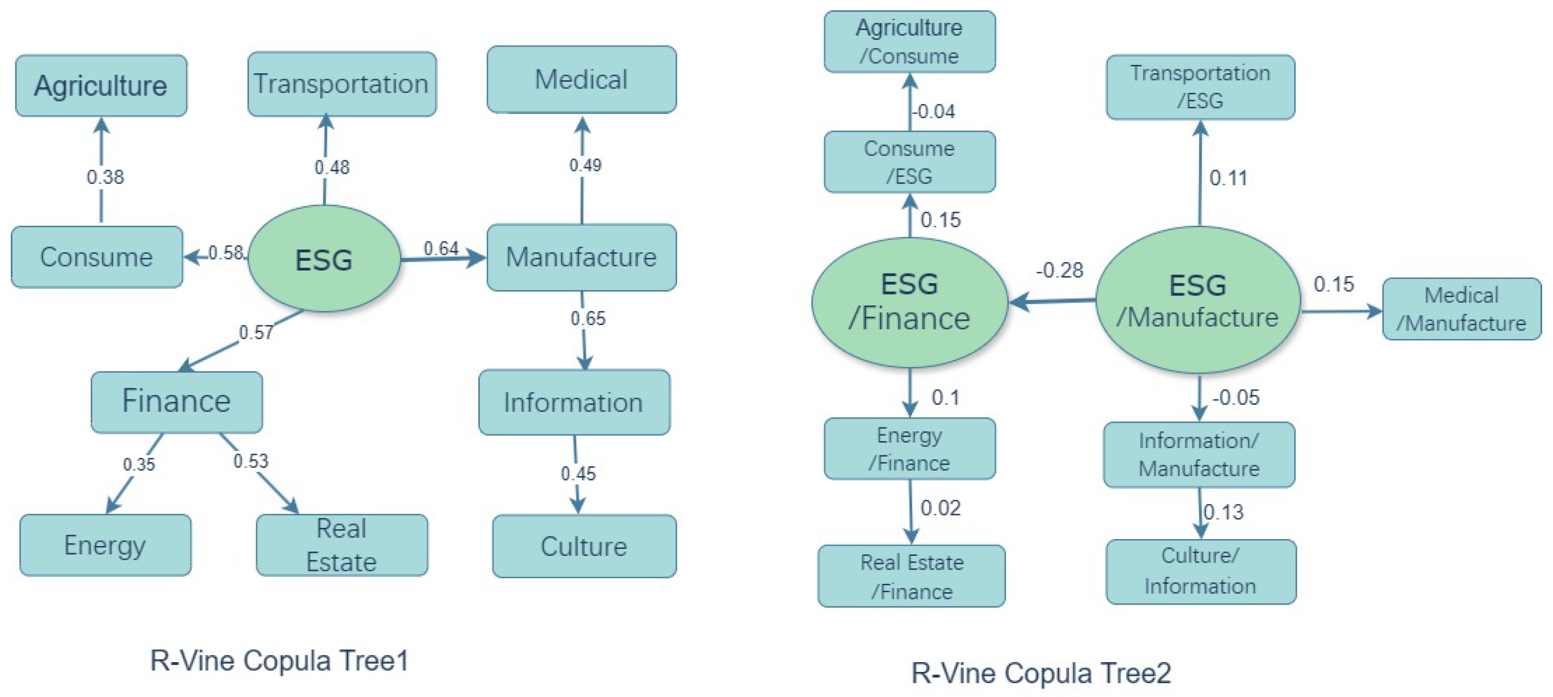
From the ARMA-eGARCH-skewed t model, the standardized residuals are derived after filtering volatility. The parameter estimates for the marginal distribution adjustment are presented in

Table 4. Marginal distribution fitting parameter estimation.

Industries	$\mathit{\mu }$	$\mathit{\omega }$	$\mathit{\alpha }$	$\mathit{\beta }$	$\mathit{\gamma }$	Skew	Shape	LLH	LB	ARCH-LM
ESG	−0.010	0.009	−0.033	0.966	0.160	0.980	6.315	−2024.173	0.173	0.466
Energy	0.059	0.011	0.051	0.988	0.104	1.028	5.515	−2391.513	0.442	0.390
Manufacturing	0.006	0.029	−0.056	0.954	0.194	0.899	9.273	−2281.310	0.068	0.899
Finance	−0.007	0.020	0.010	0.961	0.126	1.143	4.239	−2123.317	0.467	0.585
Real estate	−0.048	0.026	−0.020	0.977	0.173	1.186	4.636	−2520.924	0.089	0.109
Consumption	−0.007	0.014	−0.022	0.982	0.113	1.031	6.504	−2391.001	0.117	0.158
Agriculture	0.009	0.015	0.016	0.988	0.095	1.129	5.888	−2696.581	0.179	0.306
Medical	−0.023	0.026	−0.017	0.976	0.136	1.044	12.318	−2618.876	0.123	0.526
Transportation	−0.014	0.026	−0.028	0.966	0.128	1.041	5.491	−2333.950	0.385	0.795
Information	−0.003	0.031	−0.003	0.973	0.124	0.985	11.362	−2625.459	0.753	0.148
Culture	−0.034	0.037	−0.010	0.973	0.151	0.942	12.501	−2764.208	0.262	0.454

Note: LLH denotes the log-likelihood value, LB represents the sequence-dependent Ljung–Box statistic in the residual model, and LM is the Engle’s LM test for the ARCH effect.

.

As shown in the table, the model parameters for all industries demonstrate sound economic significance, indicating good model fit. The p-values of both the Ljung–Box (LB) test and ARCH-LM test are statistically insignificant, suggesting that the residual series exhibit no significant autocorrelation or heteroskedasticity and conform to white noise characteristics. Therefore, the marginal distribution specification is appropriate and can provide a robust foundation for subsequent Vine Copula dependence structure modeling.

4.2. Vine Copula

According to copula theory, when variables follow a uniform distribution U(0, 1), a copula function C exists, enabling the construction of the joint distribution function from the marginal distribution functions of the individual variables. To ensure the existence of the copula, the residual sequences of the industry indices, previously calculated, must undergo a probability integral transformation. The transformed sequences, which follow a uniform distribution U(0, 1), are subsequently used for modeling and analysis. The Kolmogorov–Smirnov (K-S) test is applied to evaluate whether the transformed sequences conform to a uniform distribution within the interval [0, 1]. The test results indicate that the K-S statistic for all industry index residuals is 0.00075075, with a p-value of 1, confirming that the transformed sequences follow a U(0, 1) distribution, thereby enabling subsequent Vine Copula modeling.

This study employs a Vine Copula structure, selected based on the dependency relationships among variables, to characterize the interdependencies between the ESG index and industrial sectors. The C-Vine Copula demonstrates that all industries are primarily influenced by the ESG variable, with the highest correlation coefficient observed between the manufacturing sector and the ESG index.

The C-Vine Copula tree in Figure 2 indicates that ESG serves as the dominant variable influencing all industries, underscoring its critical role in shaping industrial development. In particular, ESG exerts the strongest influence on manufacturing, consumption, and finance, with Kendall’s tau values of 0.65, 0.59, and 0.57, respectively. From the second tree (Tree 2) in the C-Vine Copula structure, it can be observed that ESG’s influence propagates primarily through the manufacturing sector before extending to other industries. This transmission pathway aligns with the sequence illustrated in the D-Vine Copula tree (see Figure 3).

The D-Vine Copula reveals the upstream–downstream transmission mechanism of the industrial chain. It begins with the upstream agricultural sector, which influences the consumption sector. ESG policies then propagate through consumption to manufacturing, with the latter further extending its influence to the information sector. The strong interdependence between manufacturing and the information sector (Kendall’s tau = 0.65) highlights the critical role of information manufacturing in driving the development of emerging industries. Traditional industries such as energy and real estate exhibit a relatively independent role within the transmission chain, demonstrating limited direct connections to the core sectors. However, they significantly influence the financial sector, likely due to the financial attributes of these industries.

The R-Vine Copula tree in Figure 4 refines the hierarchical relationships among industries, emphasizing a layered transmission effect. It identifies consumption and manufacturing as the primary nodes for the transmission of ESG policies, while other industries are indirectly influenced. In the first layer of Tree1, the sectors most directly influenced by ESG policies are manufacturing, consumption, finance, and transportation, reflecting their alignment with the sustainable development goals of consumption-driven growth and manufacturing upgrades. In Tree2 of the R-Vine Copula, manufacturing and finance emerge as the primary conduits through which ESG impacts propagate to other sectors. The coefficients in the copula structure indicate the direction and strength of these dependencies, further elucidating the nuanced interconnections among industries.

4.3. Tail Dependency

Using the tail dependence calculation formula, we derived the optimal copula types, parameter estimates, and tail dependence coefficients based on the Vine Copula structure. A deeper analysis of tail dependence relationships offers a clearer understanding of risk transmission and interdependence between the ESG benchmark index and various industries. Overall, most industries exhibit an asymmetric tail dependence structure, where lower tail dependence coefficients consistently exceed upper tail coefficients. This suggests that the system is exposed to greater risks during downturns. In terms of coefficient magnitude, manufacturing, finance, real estate, and energy exhibit higher risk values, underscoring their significant roles in tail risk. These industries require particular attention during market downturns, as they play a critical role in systemic risk events. However, sectors such as consumption, healthcare, and culture exhibit lower tail risk, indicating relative stability during market declines (

Table 5. Vine Copula parameter estimation and tail dependency.

Vine Copula	Edge	Copula	Para1	Para2	tau	Utd	Ltd
C-Vine Copula	ESG–Agriculture	SG	1.4	-	0.29	-	0.36
	ESG–Transportation	SBB1	0.22	1.75	0.48	0.16	0.51
	ESG–Medical	t	0.69	12.57	0.49	0.14	0.14
	ESG–Real Estate	SBB1	0.21	1.51	0.4	0.12	0.42
	ESG–Energy	SBB1	0.14	1.39	0.33	0.03	0.48
	ESG–Information	SBB1	0.37	1.65	0.49	0.33	0.48
	ESG–Consumption	t	0.8	24.97	0.59	0.52	0.52
	ESG–Finance	BB1	0.6	1.78	0.57	0.52	0.52
	ESG–Manufacturing	t	0.85	8	0.65	0.41	0.41
	ESG–Culture	SBB1	0.12	1.53	0.38	0.02	0.43
D-Vine Copula	Culture–Energy	SG	1.11	-	0.18	-	0.23
	Energy–Real Estate	t	0.41	5.13	0.27	0.16	0.16
	Real Estate–Finance	SBB1	0.31	1.86	0.53	0.3	0.55
	Finance–Transportation	SBB1	0.17	1.44	0.36	0.06	0.38
	Transportation–Medical	t	0.55	9.37	0.37	0.11	0.11
	Medical–Information	SBB1	0.2	1.48	0.39	0.1	0.4
	Information–Manufacturing	t	0.85	7.24	0.65	0.44	0.44
	Manufacture-ESG	t	0.85	8	0.65	0.41	0.41
	ESG–Consumption	t	0.8	24.97	0.59	0.1	0.1
	Consumption–Agriculture	SBB1	0.26	1.43	0.38	0.16	0.37
R-Vine Copula	ESG–Manufacturing	t	0.85	8	0.64	0.41	0.41
	ESG–Finance	BB1	0.59	1.79	0.57	0.53	0.54
	ESG–Consumption	t	0.79	26.62	0.58	0.09	0.09
	ESG–Transportation	Survival BB1	0.21	1.74	0.48	0.15	0.51
	Manufacture–Information	t	0.85	7.23	0.65	0.44	0.44
	Information–Culture	t	0.65	8	0.45	0.2	0.2
	Manufacture–Medical	t	0.69	11.57	0.49	0.15	0.15
	Finance–Real estate	Survival BB1	0.32	1.84	0.53	0.31	0.54
	Finance–Energy	Survival BB1	0.16	1.43	0.35	0.04	0.38
	Consumption–Agriculture	Survival BB1	0.26	1.43	0.38	0.15	0.37

Note: tau represents Kendall’s $\tau$; Utd represents upper tail dependency; and Ltd represents lower tail dependency.

).

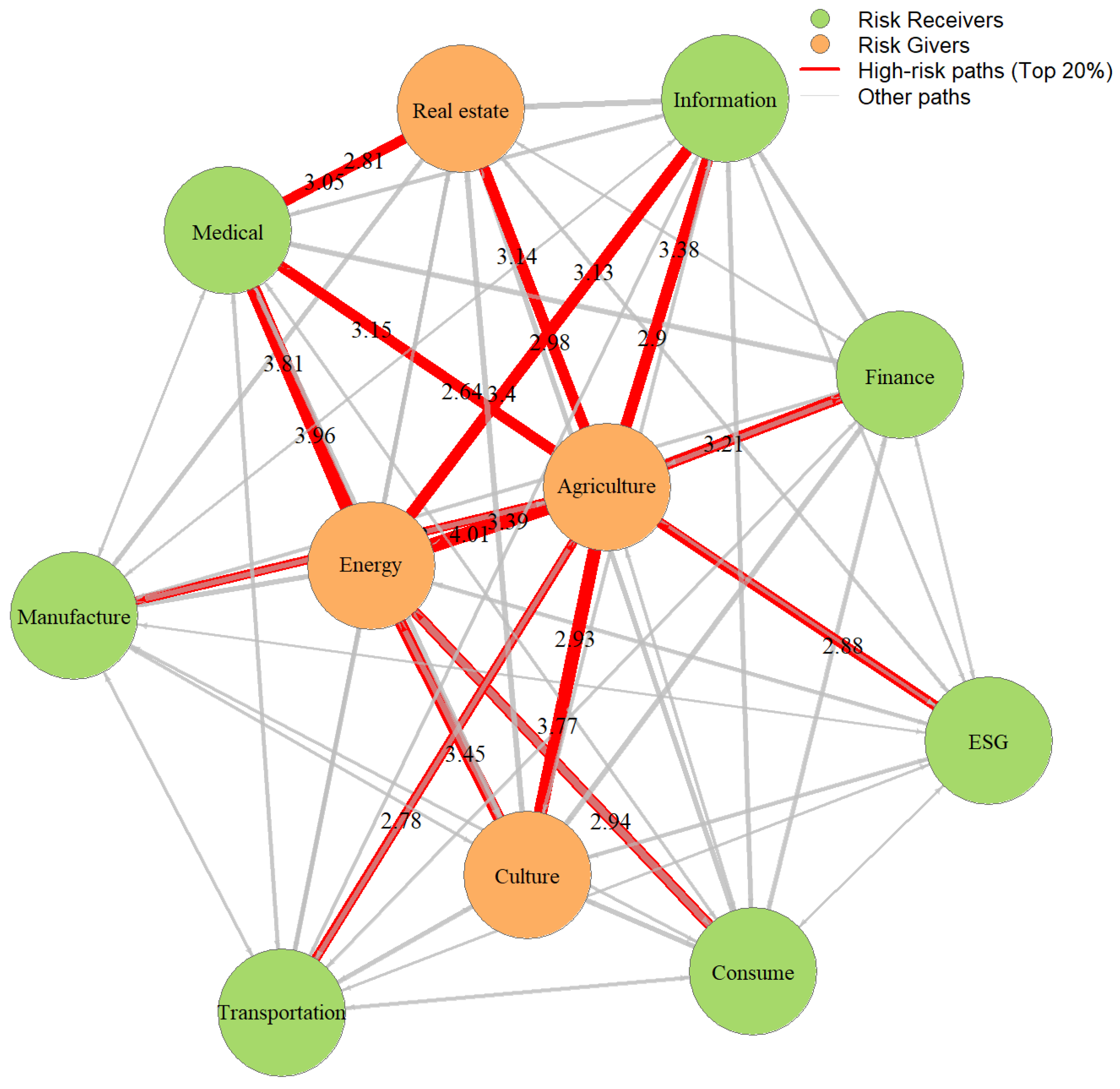
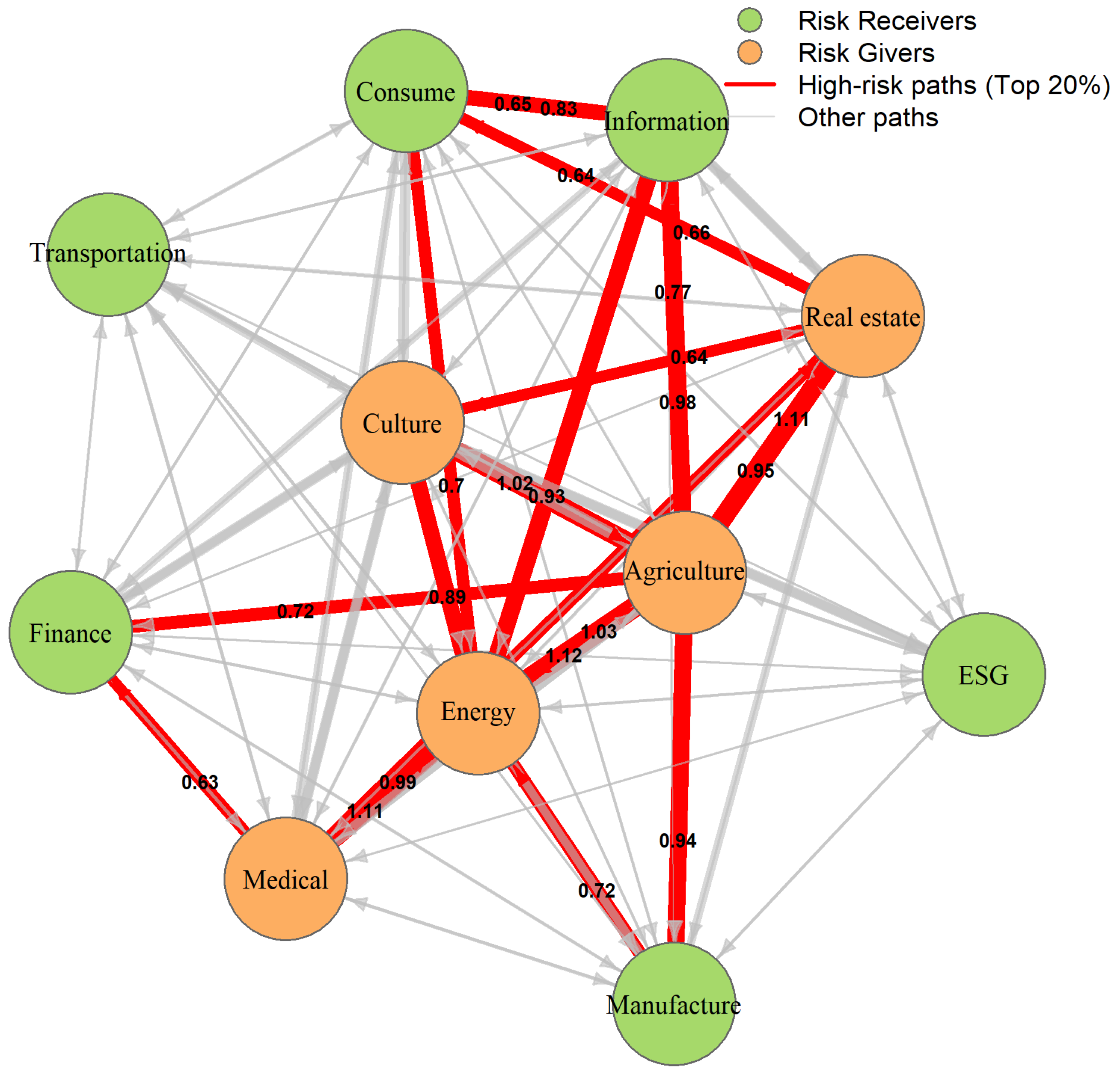
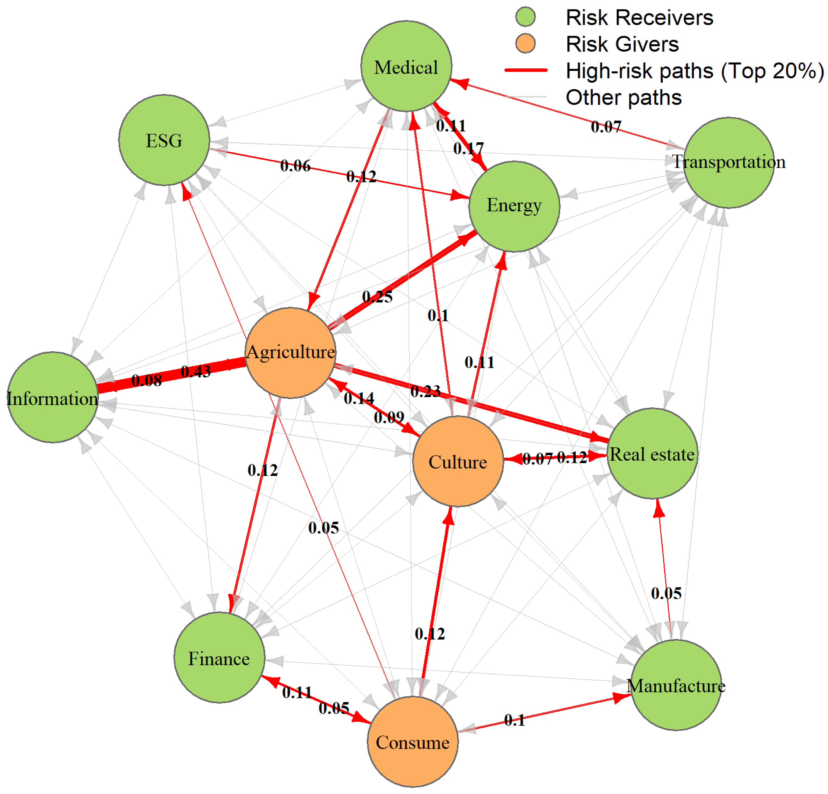
4.4. Risk Spillover Analysis by CoVaR

To investigate the hierarchical spillover effects of risk, this study employs the R-Vine Copula model combined with Monte Carlo simulation. By generating 10,000 sets of return series, the losses for each industry were calculated under various scenarios. Based on these simulations, the Value at Risk (VaR) and Conditional Value at Risk (CoVaR) for each industry were estimated, offering insights into the risks faced by different industries under extreme market conditions.

4.4.1. VaR Analysis

Based on the estimated Value at Risk (VaR) across different sectors, notable heterogeneity emerges in their exposure to extreme market conditions (see

Table 6. VaR values at different levels for each industry.

Industries	90%	95%	99%
ESG	0.099	0.051	0.010
Energy	0.102	0.051	0.009
Manufacturing	0.098	0.053	0.008
Finance	0.102	0.048	0.009
Real estate	0.101	0.049	0.010
Consumption	0.101	0.049	0.010
Agriculture	0.102	0.054	0.011
Medical	0.096	0.049	0.009
Transportation	0.103	0.050	0.011
Information	0.099	0.054	0.009
Culture	0.103	0.048	0.009

). The energy sector exhibits relatively elevated VaR values across all confidence levels, reflecting its strong sensitivity to international energy price fluctuations. The manufacturing sector shows heightened risk exposure, likely due to its heavy reliance on upstream raw materials, downstream demand volatility, and its susceptibility to ESG-related regulations such as carbon emission constraints. The real estate sector registers one of the highest VaR values at the 99% confidence level (1.0%), highlighting its vulnerability to market shocks, which can be attributed to its dependence on financing accessibility and cyclical market dynamics. In contrast, the information and cultural industries present comparatively lower VaR values, suggesting stronger resilience under stress scenarios. This can be explained by their asset-light structures, high levels of technological value-added, and relatively stable global demand. These findings lay the foundation for subsequent CoVaR analysis, which captures not only individual sector risk but also the systemic spillover effects stemming from inter-sectoral dependencies under extreme market conditions.

4.4.2. CoVaR Analysis

The essence of Value at Risk (VaR) lies in identifying the lower $\alpha$-quantile of the distribution function F. Building on VaR, we compute the Conditional Value at Risk (CoVaR), which quantifies the risk level of a specific industry conditional on another industry being under extreme conditions. A higher CoVaR value indicates a stronger risk spillover effect from one industry to another under adverse conditions, whereas a lower CoVaR value reflects a weaker spillover effect. By analyzing the CoVaR matrix below, we can evaluate the effects of risk transmission among industries and, in conjunction with the C-vine, D-vine, and R-Vine Copula models, identify industries with strong risk dependencies.

At the 90% confidence level, the agriculture sector exhibits relatively high CoVaR values (see

Table 7. CoVaR values at 90% confidence level.

Industries	ESG	Energy	Manufacturing	Finance	Real Estate	Consumption	Agriculture	Medical	Transportation	Information	Culture
ESG	NA	1.498	1.119	1.267	1.319	1.134	2.876	1.360	1.107	1.116	1.488
Energy	1.708	NA	1.928	1.523	1.817	2.540	4.009	3.959	1.634	3.404	2.340
Manufacturing	0.923	1.916	NA	1.554	1.907	1.150	2.059	1.095	1.519	0.995	1.244
Finance	0.806	1.365	1.334	NA	1.182	1.392	2.058	1.637	1.386	1.981	2.083
Real estate	1.371	1.700	1.746	1.150	NA	2.137	3.145	2.809	1.285	2.464	2.503
Consumption	1.109	2.936	1.329	2.038	1.962	NA	1.354	1.162	1.249	2.005	1.961
Agriculture	1.899	3.394	2.716	3.206	2.976	1.242	NA	2.639	2.134	2.905	2.932
Medical	1.081	3.806	1.089	2.236	3.049	1.373	3.148	NA	1.497	1.430	1.613
Transportation	1.119	1.966	0.963	1.237	1.549	1.579	2.777	1.785	NA	1.482	1.953
Information	1.366	3.128	1.127	1.698	2.368	1.817	3.382	1.585	1.307	NA	1.528
Culture	1.822	3.450	1.532	2.198	2.066	2.071	3.767	2.068	1.751	1.383	NA

Note: The table shows the CoVaR values (×100). Rows represent sectors whose distress influences other sectors; columns represent sectors whose risk is influenced by the distress in other sectors. NA indicates missing values where a sector cannot influence itself.

), indicating its prominent role as a risk amplifier within upstream segments of the supply chain. The manufacturing and energy sectors also present elevated risk levels, with CoVaR values of 0.271 and 0.264, respectively. These heightened risks can be attributed to their pronounced exposure to supply-side shocks and policy-driven pressures, particularly those arising from ESG-related regulations. The real estate sector demonstrates a moderate risk level (CoVaR = 0.275), largely influenced by financing constraints and fluctuations in market sentiment. In contrast, sectors including information technology, cultural industries, and transportation exhibit relatively lower CoVaR values (below 0.2), reflecting greater stability under normal market conditions.

The corresponding risk spillover network (see Figure 5) at the 90% level visually confirms these findings: nodes representing agriculture, energy, real estate, and culture occupy central positions with multiple outgoing edges, signifying their significant spillover effects on other sectors. Conversely, the peripheral positioning of sectors like information and transportation suggests weaker inter-sectoral risk transmission in typical market conditions.

At the 95% confidence level, the CoVaR values (see

Table 8. CoVaR values at 95% confidence level.

Industries	ESG	Energy	Manufacturing	Finance	Real Estate	Consumption	Agriculture	Medical	Transportation	Information	Culture
ESG	NA	0.350	0.377	0.246	0.273	0.417	0.427	0.248	0.236	0.331	0.486
Energy	0.303	NA	0.477	0.351	0.422	0.695	1.121	0.989	0.372	0.928	0.888
Manufacturing	0.352	0.722	NA	0.303	0.468	0.313	0.938	0.365	0.290	0.180	0.330
Finance	0.294	0.330	0.414	NA	0.247	0.377	0.719	0.410	0.356	0.292	0.451
Real estate	0.396	0.297	0.300	0.288	NA	0.655	1.109	0.376	0.450	0.488	0.641
Consumption	0.305	0.463	0.357	0.377	0.642	NA	0.213	0.335	0.304	0.646	0.364
Agriculture	0.450	1.031	0.504	0.393	0.950	0.371	NA	0.623	0.443	0.984	0.611
Medical	0.274	1.107	0.384	0.634	0.653	0.490	0.616	NA	0.403	0.346	0.581
Transportation	0.299	0.446	0.275	0.225	0.285	0.449	0.438	0.357	NA	0.325	0.496
Information	0.295	0.555	0.286	0.473	0.597	0.834	0.770	0.381	0.374	NA	0.328
Culture	0.588	0.587	0.278	0.589	0.454	0.577	1.024	0.480	0.361	0.415	NA

Note: The table shows the CoVaR values (×100). Rows represent sectors whose distress influences other sectors; columns represent sectors whose risk is influenced by the distress in other sectors. NA indicates missing values where a sector cannot influence itself.

) increase substantially, especially in agriculture (0.395) and culture (0.374). This indicates that, under moderately stressed conditions, cultural industries, despite their asset-light business model, remain susceptible to broader systemic shocks, possibly due to demand-side vulnerabilities and cyclical investments in digital infrastructure. Similarly, manufacturing (0.349) and energy (0.335) continue to play central roles in risk propagation, underscoring their upstream positioning in the supply chain and exposure to ESG-related transitions.

The real estate sector (0.344) exhibits heightened volatility, reflecting its dual dependence on macroeconomic cycles and financing conditions. Of particular note is the consumer sector (0.320), which begins to show increased vulnerability, suggesting amplified downstream exposure to risks transmitted from upstream industries such as energy and manufacturing.

The risk spillover network at this level reveals a denser structure with enhanced connectivity (see Figure 6). Notably, agriculture and energy sectors emerge as dominant sources of systemic risk, occupying central positions with multiple outgoing links to downstream industries. This underlines their pivotal roles in initiating and propagating shocks across the supply chain. The cultural sector, previously peripheral, now emerges as a more interconnected node, indicating its rising systemic relevance. The agriculture and manufacturing sectors remain core risk transmitters with intensified interlinkages, reflecting the growing contagion potential under moderate stress.

At the 99% confidence level, systemic risks become sharply more pronounced (see

Table 9. CoVaR values at 99% confidence level.

Industries	ESG	Energy	Manufacturing	Finance	Real Estate	Consumption	Agriculture	Medical	Transportation	Information	Culture
ESG	NA	0.062	0.012	0.040	0.004	0.015	0.012	0.041	0.041	0.015	0.009
Energy	0.013	NA	0.039	0.001	0.044	0.011	0.027	0.175	0.047	0.010	0.013
Manufacturing	0.024	0.011	NA	0.038	0.052	0.010	0.004	0.025	0.026	0.008	0.015
Finance	0.007	0.014	0.022	NA	0.018	0.109	0.028	0.008	0.027	0.017	0.037
Real estate	0.019	0.029	0.027	0.023	NA	0.033	0.013	0.004	0.033	0.013	0.122
Consumption	0.054	0.050	0.097	0.052	0.046	NA	0.008	0.018	0.006	0.031	0.121
Agriculture	0.032	0.253	0.018	0.117	0.229	0.003	NA	0.039	0.026	0.427	0.137
Medical	0.016	0.106	0.030	0.020	0.033	0.005	0.117	NA	0.014	0.051	0.033
Transportation	0.015	0.031	0.014	0.034	0.013	0.019	0.014	0.068	NA	0.008	0.026
Information	0.040	0.011	0.020	0.020	0.014	0.011	0.078	0.014	0.009	NA	0.029
Culture	0.023	0.108	0.023	0.032	0.075	0.013	0.094	0.096	0.028	0.003	NA

Note: The table shows the CoVaR values (×100). Rows represent sectors whose distress influences other sectors; columns represent sectors whose risk is influenced by the distress in other sectors. NA indicates missing values where a sector cannot influence itself.

). The real estate sector registers the highest CoVaR (1.04%), emphasizing its acute sensitivity to financial tightening, asset devaluation, and liquidity stress during extreme market conditions. Energy (0.392) and manufacturing (0.377) also exhibit elevated CoVaR values, highlighting their critical roles in absorbing and transmitting shocks related to input prices and ESG transition pressures.

The agriculture sector (0.427) maintains its high risk transmission capacity, consistent with its foundational role in food security and cost-push inflation. The cultural industry (0.486), unexpectedly, demonstrates strong systemic connectivity—likely due to its linkages with media, digital economy platforms, and consumption behavior. Conversely, sectors such as information technology (0.293) and transportation (0.267) appear more resilient, benefiting from digital transformation and operational flexibility (Figure 7).

The corresponding risk network diagram at the 99% level reveals a densely interconnected structure; the degree of outgoing and incoming edges increases significantly, indicating intensified systemic contagion. The network highlights a more fragile and interdependent industrial structure under extreme stress, with the agriculture sector acting as hubs in risk transmission paths.

Integrating the Vine Copula dependence structure with CoVaR-based risk spillover estimates, we identify ESG as a primary systemic trigger, exerting direct influence on agriculture, energy, manufacturing, consumer, and cultural sectors. Under extreme ESG-related stress, agriculture emerges as a key transmission node (as captured by the D-vine structure), propagating risks toward finance, real estate, healthcare, and downstream consumption through cost-push mechanisms.

In the conditional R-vine dependence network, manufacturing assumes a pivotal role, acting as a conduit linking ESG shocks to downstream sectors such as energy (0.722), real estate (0.468), and healthcare (0.365). The energy sector, being resource-intensive, also plays a substantial risk propagation role, most notably to real estate (0.950) and healthcare (1.107), highlighting the systemic vulnerabilities arising from energy price volatility or supply disruptions.

The real estate sector functions both as a risk receiver and mediator, amplifying shocks through financing and asset valuation channels. In contrast, consumer, transportation, and information industries display comparatively greater resilience, as evidenced by limited CoVaR spillover across both confidence levels.

In summary, the multi-layered CoVaR analysis, combined with the Vine Copula dependence framework, effectively reveals sectoral heterogeneity in systemic risk exposure and transmission dynamics under varying market stress scenarios.

4.5. Robustness Check Based on Confidence Levels

To ensure the robustness of the risk spillover results, this study further investigates the consistency of spillover roles across different confidence levels (90%, 95%, and 99%) using the CoVaR-based spillover values. The objective is to test whether industries maintain stable spillover directions (giver/receiver) and magnitudes under varying tail risk thresholds.

As shown in

Table 10. Risk spillover effects at different confidence levels.

Level	Type	ESG	Energy	Manufacturing	Finance	Real Estate	Consumption	Agriculture	Medical	Transportation	Information	Culture
90%	Risk_Out	0.778	0.650	1.569	1.844	0.855	1.578	−1.533	2.989	0.456	1.850	0.074
	Risk_In	−4.396	7.390	−4.228	−3.074	2.321	−1.332	9.131	2.111	−2.072	1.115	4.143
	Net	−5.174	6.740	−5.797	−4.917	1.467	−2.910	10.664	−0.878	−2.528	−0.735	4.069
	Role	R	G	R	R	G	R	G	R	R	R	G
95%	Risk_Out	0.513	0.799	−0.019	0.239	0.380	0.484	−0.072	0.778	−0.075	1.131	0.265
	Risk_In	−1.140	2.218	−0.208	−0.581	0.623	−0.359	2.269	1.031	−0.875	0.437	1.008
	Net	−1.653	1.419	−0.189	−0.820	0.243	−0.843	2.341	0.252	−0.800	−0.694	0.744
	Role	R	G	R	R	G	R	G	G	R	R	G
99%	Risk_Out	0.034	0.270	0.075	0.046	0.144	0.107	0.194	0.167	−0.008	0.444	0.232
	Risk_In	−0.020	0.129	−0.055	0.030	0.062	0.203	1.009	0.166	−0.024	−0.031	0.236
	Net	−0.055	−0.141	−0.130	−0.016	−0.082	0.097	0.815	−0.001	−0.016	−0.475	0.004
	Role	R	R	R	R	R	G	G	R	R	R	G

Note: R represents risk receivers (net risk inflow); G represents risk givers (net risk outflow).

, most industries demonstrate consistent risk roles across confidence levels. Agriculture, culture, and energy consistently act as net risk givers, particularly evident at the 90% and 95% levels, suggesting their stable systemic influence across moderate to extreme market stress. Conversely, finance, manufacturing, and ESG-related industries remain net receivers, indicating their persistent vulnerability to external shocks. Consumption and medical sectors exhibit mild role shifts across confidence levels, indicating a context-dependent spillover pattern, possibly influenced by market sentiment and policy interventions during extreme events. At the 99% level, the magnitude of net spillovers tends to narrow for most industries, reflecting the tail-thinning effect in extreme quantiles. This is particularly notable for energy, which switches from being a net giver at 90%/95% to a net receiver at 99%, suggesting that its spillover role weakens under extreme stress, possibly due to its hedging function or market saturation.

These results confirm the robustness of the overall spillover structure, while also highlighting a few sensitive sectors whose risk roles depend on the depth of market shocks.

5. Discussion

Based on the research findings, we propose policy recommendations centered on ESG principles, with a focus on targeted measures aligned with identified risk transmission nodes.

Manufacturing Sector (Supply-Side Reform): Given its centrality and conditional dependence on energy and real estate, manufacturing reform should emphasize green upgrading, promoting cleaner production processes, investing in industrial digitalization, and enhancing energy efficiency. Policies should also incentivize circular economy practices in high-impact subsectors like chemicals and heavy industries.

Consumption and Financial Services (Demand-Side Promotion): To enhance downstream market stability, governments should implement targeted fiscal subsidies or tax incentives to stimulate green consumption. Meanwhile, financial institutions should be encouraged to develop ESG-aligned investment products, improving capital allocation toward low-risk and low-carbon sectors.

Agricultural and Energy Sectors (Risk Transmission Origins): As upstream risk transmitters, agriculture and energy require resilience-oriented interventions. For agriculture, this includes strengthening supply chain digital infrastructure, improving climate-resilient farming systems, and establishing national grain reserve mechanisms. For energy, dynamic hedging instruments and energy mix diversification can be used to absorb volatility and reduce contagion to downstream industries.

Tail Risk Management: The observed asymmetric tail dependencies necessitate sector-specific stress testing and early warning systems, especially in real estate and manufacturing. Promoting cross-sector collaboration can help mitigate systemic shocks under extreme scenarios.

While this study provides valuable insights into inter-industry dependency structures and presents an analytical framework well suited for capturing nonlinear dependencies and tail risk spillovers, certain limitations must be acknowledged. First, the analysis relies on a static sample and does not fully account for structural breaks or transitions in market dynamics. Future research could incorporate dynamic models with regime-switching features, such as Markov switching copulas or time-varying Vine Copulas [39], to better reflect evolving inter-sector relationships. Second, the current study adopts a domestic perspective focused on China’s industrial system. Given the globalization of supply chains and ESG policy spillovers, future research should explore cross-border interdependencies by extending the framework to include international sectors and ESG-related transmission channels [23]. This would enhance the understanding of systemic risks in a globally interconnected industrial ecosystem and offer broader policy implications under the global ESG transition.

6. Conclusions

This study employs advanced econometric methods to measure and analyze dependency structures among industries and risk spillovers. The selected approaches—ARMA-eGARCH with skewed t-distribution, Vine Copula models (C-vine, D-vine, R-vine), tail dependence analysis, and CoVaR spillover measures—were used to comprehensively investigate inter-industry dependence structures and systemic risk transmission under ESG-driven transitions. These methods, each targeting distinct aspects of financial interconnectedness and nonlinearity, collectively construct a robust analytical framework to evaluate structural vulnerabilities within industrial systems.

The study identifies several key findings:

(1) Dependence Structures in the Industrial Chain: The analysis reveals a prominent ESG-centered industrial chain with significant dependence across key sectors. The manufacturing sector plays a pivotal mediating role ($\tau$ = 0.64), showing strong interconnections with energy, real estate, and pharmaceuticals, consistent with its core position in China’s supply-side reform strategy. Consumption ($\tau$ = 0.58) and financial sectors ($\tau$ = 0.57) also demonstrate substantial dependence, reflecting their role in supporting demand-side stimulation and risk absorption. Manufacturing, as a secondary central node, exhibits significant conditional dependence on the energy, real estate, and pharmaceutical industries, underscoring its critical role in supply-side reforms. These findings align with China’s emphasis on supply-side structural reforms and demand-stimulating policies.

(2) Tail Dependence Analysis: Most industries exhibit asymmetric tail dependence, characterized by greater risk spillovers during market downturns (e.g., Survival Gumbel and Survival Clayton–Gumbel copulas). The real estate sector exhibits the highest Value at Risk (VaR) in extreme conditions (1.04% at the 99% confidence level), indicating its heightened vulnerability to systemic shocks. In contrast, the information and cultural industries, due to their asset-light and high-tech nature, exhibit greater resilience and lower risk spillover values.

(3) Risk Spillovers: CoVaR analysis reveals a clear upstream-to-downstream risk propagation path: “agriculture → energy → manufacturing → finance → consumption → culture industries”. Agriculture emerges as a primary risk transmitter, while manufacturing and finance act as amplifiers. This chain underscores the importance of targeted interventions in upstream sectors to contain systemic risk.

The findings highlight the transformative potential of ESG policies in reshaping industrial dynamics and mitigating systemic risks. Understanding the interconnections among industries and ESG frameworks, as well as dependency structures and risk spillover pathways, can enhance economic resilience and competitiveness. This research provides actionable insights to support the green transformation of industries and the development of a sustainable economic system.

References

1. Alharbi, F. The Impact of ESG Reforms on Economic Growth in GCC Countries: The Role of Financial Development. Sustainability 2024, 16, 11067. [Google Scholar] [CrossRef]
2. Eccles, R.G.; Serafeim, G.; Seth, D.; Ming, C.C.Y. The Performance Frontier: Innovating for a Sustainable Strategy: Interaction. Harv. Bus. Rev. 2013, 91, 17–18. [Google Scholar]
3. Wu, Y.; Ivashkovskaya, I.; Besstremyannaya, G.; Liu, C. Unlocking Green Innovation Potential Amidst Digital Transformation Challenges—The Evidence from ESG Transformation in China. Sustainability 2025, 17, 309. [Google Scholar] [CrossRef]
4. Liu, Z.; Deng, Z.; He, G.; Wang, H.; Zhang, X.; Lin, J.; Liang, X. Challenges and opportunities for carbon neutrality in China. Nat. Rev. Earth Environ. 2022, 3, 141–155. [Google Scholar] [CrossRef]
5. Liu, Z.; Zhou, Q. The Pressure of Carbon Loss in Industrial Upgrading: Pathways and Challenges of Low-Carbon Transition in China’s Manufacturing Sector. Law Econ. 2024, 3, 54–64. [Google Scholar] [CrossRef]
6. Traverso, M. ESG and Systemic Risk, the Mitigation Effect of ESG on Systemic Risk Using a Network Approach. 2024. Available online: https://unitesi.unive.it/handle/20.500.14247/23123 (accessed on 21 October 2024).
7. Chong, Z.L. Environmental, Social and Governance (ESG) Practices in Construction Supply Chain Organisations: A Comparison of Organisational Practices and Cognitive Perceptions of Industrial Practitioners. Ph.D. Thesis, UTAR, Petaling Jaya, Malaysia, 2024. [Google Scholar]
8. Kotsantonis, S.; Serafeim, G. Four things no one will tell you about ESG data. J. Appl. Corp. Financ. 2019, 31, 50–58. [Google Scholar] [CrossRef]
9. Scholtens, B. Why finance should care about ecology. Trends Ecol. Evol. 2017, 32, 500–505. [Google Scholar] [CrossRef]
10. Cruz, C. The Impact of ESG Policies on Macroeconomic Volatility. Int. Rev. Econ. Financ. 2019, 64, 12–25. [Google Scholar]
11. Wei, J.; Hu, R.; Chen, F. The Path to Sustainable Stability: Can ESG Investing Mitigate the Spillover Effects of Risk in China’s Financial Markets? Sustainability 2024, 16, 10316. [Google Scholar] [CrossRef]
12. Wang, X.; Wu, H.; Shen, Y.; Wang, T. Towards Sustainable Supply Chains: Evaluating the Role of Supply Chain Diversification in Enhancing Corporate ESG Performance. Systems 2025, 13, 266. [Google Scholar] [CrossRef]
13. Fourgon, Y. The Global Impact of Mandatory ESG Disclosure on the Cost of Capital: A Comparative Analysis Across Legal Regimes. 2024. Available online: https://matheo.uliege.be/bitstream/2268.2/19920/4/23%20Master%20Thesis%20-%20Fourgon%20Ysaline.pdf (accessed on 25 July 2024).
14. Lins, K.V.; Servaes, H.; Tamayo, A. Social capital, trust, and firm performance: The value of corporate social responsibility during the financial crisis. J. Financ. 2017, 72, 1785–1824. [Google Scholar] [CrossRef]
15. Kramer, M.R.; Porter, M. Creating Shared Value; FSG: Boston, MA, USA, 2011; Volume 17. [Google Scholar]
16. Liu, L. Impact of firm ESG performance on cost of debt: Insights from the Chinese Bond Market. Macroecon. Financ. Emerg. Mark. Econ. 2024, 1–20. [Google Scholar] [CrossRef]
17. Lööf, H.; Sahamkhadam, M.; Stephan, A. Incorporating ESG into optimal stock portfolios for the global timber & forestry industry. J. For. Econ. 2023, 38, 133–157. [Google Scholar]
18. Dong, F.; Li, Z.; Huang, Z.; Liu, Y. Extreme weather, policy uncertainty, and risk spillovers between energy, financial, and carbon markets. Energy Econ. 2024, 137, 107761. [Google Scholar] [CrossRef]
19. Sklar, M. Fonctions de répartition à n dimensions et leurs marges. Ann. l’ISUP 1959, 8, 229–231. [Google Scholar]
20. Joe, H. Multivariate Models and Multivariate Dependence Concepts; CRC Press: Boca Raton, FL, USA, 1997. [Google Scholar]
21. Embrechts, P. Correlation and Dependence in Risk Management: Properties and Pitfalls. In Risk Management: Value at Risk and Beyond; Cambridge University Press: Cambridge, UK, 2002. [Google Scholar]
22. Bedford, T.; Cooke, R.M. Probability density decomposition for conditionally dependent random variables modeled by vines. Ann. Math. Artif. Intell. 2001, 32, 245–268. [Google Scholar] [CrossRef]
23. Czado, C.; Bax, K.; Sahin, Ö.; Nagler, T.; Min, A.; Paterlini, S. Vine copula based dependence modeling in sustainable finance. J. Financ. Data Sci. 2022, 8, 309–330. [Google Scholar] [CrossRef]
24. Tobias, A.; Brunnermeier, M.K. CoVaR. Am. Econ. Rev. 2016, 106, 1705. [Google Scholar]
25. Demartis, S.; Rogo, B. The Relationship Between ESG Scores and Value-at-Risk: A Vine Copula–GARCH Based Approach. J. Risk Financ. Manag. 2024, 17, 517. [Google Scholar] [CrossRef]
26. Thornqvist, V. Effects of ESG on Market Risk: A Copula and a Regression Approach to CoVaR. 2023. Available online: https://www.diva-portal.org/smash/record.jsf?pid=diva2:1765155 (accessed on 13 June 2023).
27. Bollerslev, T. Generalized Autoregressive Conditional Heteroskedasticity. J. Econom. 1986, 31, 307–327. [Google Scholar] [CrossRef]
28. Nelson, D.B. Conditional heteroskedasticity in asset returns: A new approach. Econom. J. Econom. Soc. 1991, 59, 347–370. [Google Scholar] [CrossRef]
29. Joe, H. Dependence Modeling with Copulas; CRC Press: Boca Raton, FL, USA, 2014. [Google Scholar]
30. Trivedi, P.K.; Zimmer, D.M. Copula modeling: An introduction for practitioners. Found. Trends Econom. 2007, 1, 1–111. [Google Scholar] [CrossRef]
31. Genest, C.; MacKay, J. The Joy of Copulas: Bivariate Distributions with Uniform Marginals. Am. Stat. 1986, 40, 280–283. [Google Scholar] [CrossRef]
32. Song, Y.; Ori-McKenney, K.M.; Zheng, Y.; Han, C.; Jan, L.Y. Regeneration of Drosophila sensory neuron axons and dendrites is regulated by the Akt pathway involving Pten and microRNA bantam. Genes Dev. 2012, 26, 1612–1625. [Google Scholar] [CrossRef]
33. Demarta, S.; McNeil, A.J. The t copula and related copulas. Int. Stat. Rev. 2005, 73, 111–129. [Google Scholar] [CrossRef]
34. Gudendorf, G.; Segers, J. Extreme-value copulas. In Copula Theory and Its Applications, Proceedings of the Workshop, Warsaw, Poland, 25–26 September 2009; Springer: Berlin/Heidelberg, Germany, 2010; pp. 127–145. [Google Scholar]
35. Salvadori, A.; Gray, L.J. Analytical integrations and SIFs computation in 2D fracture mechanics. Int. J. Numer. Methods Eng. 2007, 70, 445–495. [Google Scholar] [CrossRef]
36. Kendall, M.G. A new measure of rank correlation. Biometrika 1938, 30, 81–93. [Google Scholar] [CrossRef]
37. Nelsen, R.B. An Introduction to Copulas, 2nd ed.; Springer: Berlin/Heidelberg, Germany, 2006. [Google Scholar] [CrossRef]
38. Diebold, F.X.; Yilmaz, K. Better to give than to receive: Predictive directional measurement of volatility spillovers. Int. J. Forecast. 2012, 28, 57–66. [Google Scholar] [CrossRef]
39. Afzal, F.; Pan, H.; Afzal, F.; Gul, R.F. Analyzing risk contagion and volatility spillover across multi-market capital flow using EVT theory and C-vine Copula. Heliyon 2024, 10, e39918. [Google Scholar] [CrossRef]
Figure 1. The index of each industries.
Sustainability 17 04660 g001
Figure 2. C-Vine Copula Tree1 and Tree2.
Sustainability 17 04660 g002
Figure 3. D-Vine Copula Tree1.
Sustainability 17 04660 g003
Figure 4. R-Vine Copula Tree1 and Tree2.
Sustainability 17 04660 g004
Figure 5. The risk spillover path at 90% level.
Sustainability 17 04660 g005
Figure 6. The risk spillover path at 95% level.
Sustainability 17 04660 g006
Figure 7. The risk spillover path at 99% level.
Sustainability 17 04660 g007