


Research on Resource Consumption Standards for Highway Electromechanical Equipment Based on Monte Carlo Model

Abstract
1. Introduction
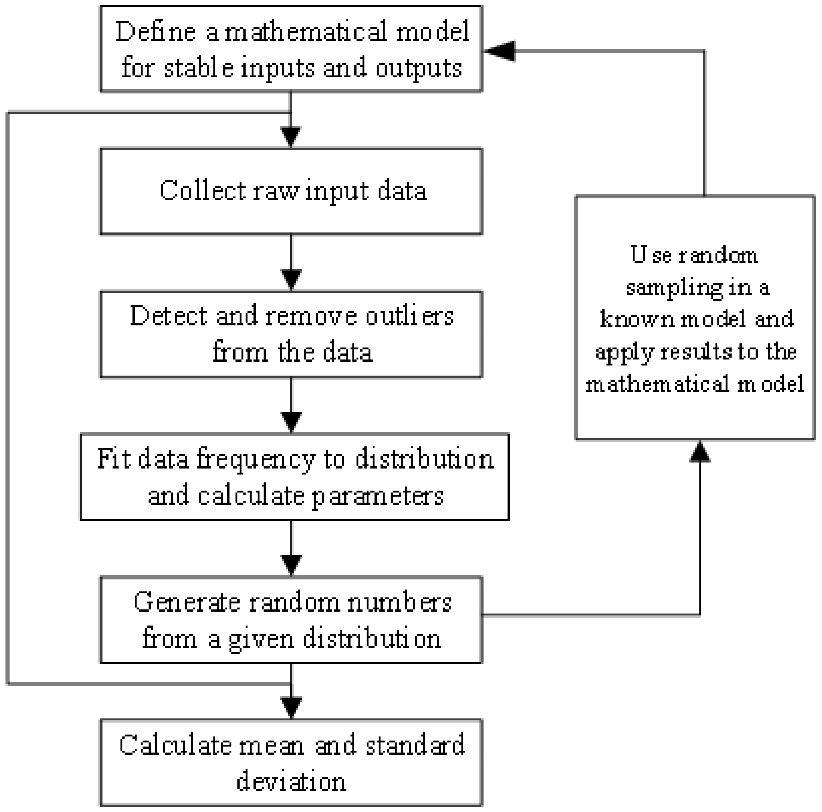
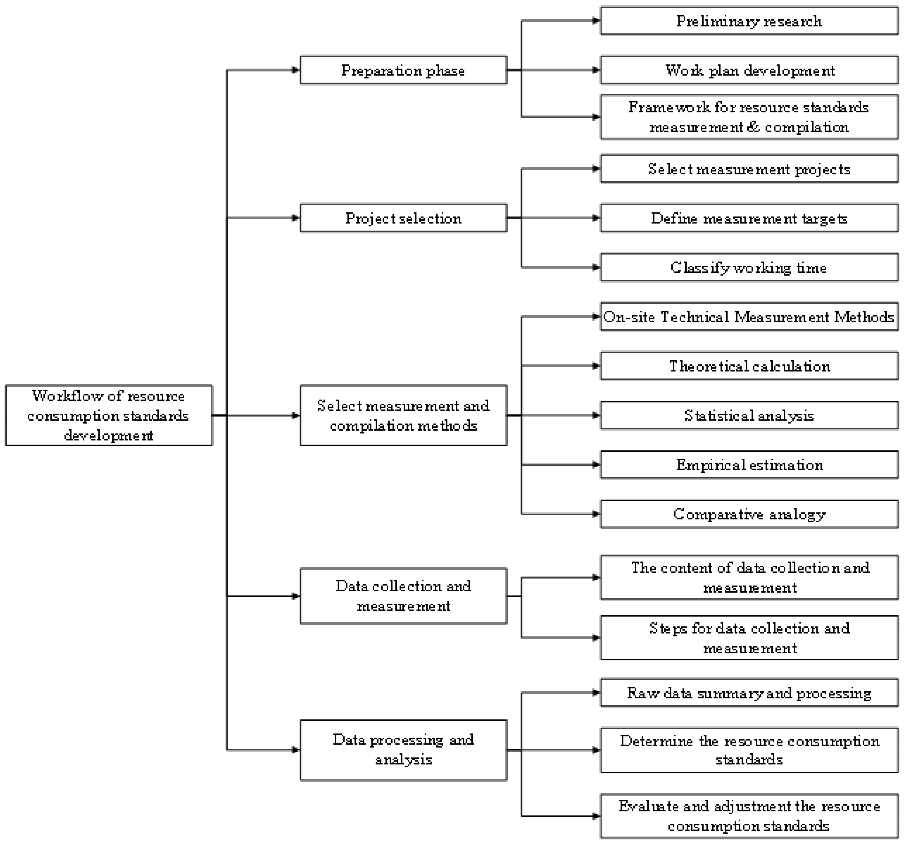
2. Methods
2.1. Monte Carlo Method Overview
2.2. Model Construction for Highway Electromechanical Equipment Resource Consumption Standards
2.2.1. Data Collection and Processing
Raw Data Collection
Error Classification and Characteristics
Error Processing Methods
2.2.2. Establishing the Probability Distribution Function Model and Analysis
2.2.3. Data Simulation
2.2.4. Monte Carlo Simulation Results and Accuracy Analysis
2.3. Validation Analysis of Standardized Cost Benchmarks for Expressway Electromechanical Systems
2.3.1. Compliance with the Price of National Construction Standards
2.3.2. Compliance with Market Price
3. Results and Discussion
3.1. Data Sources
3.2. Results of National Construction Standards for Resource Consumption Standards
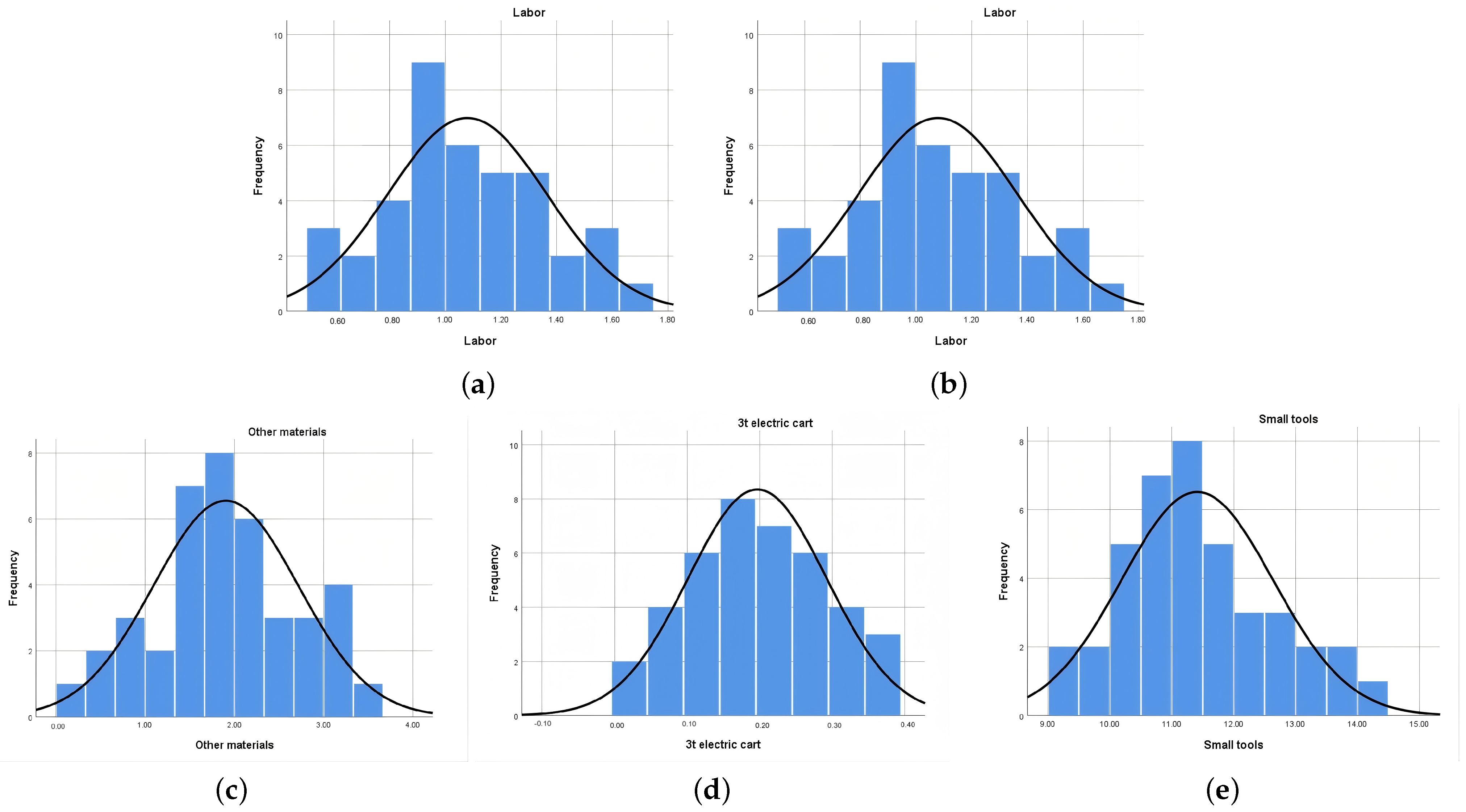
3.3. Results of Data Collection
3.4. Results of Outlier Identification and Elimination
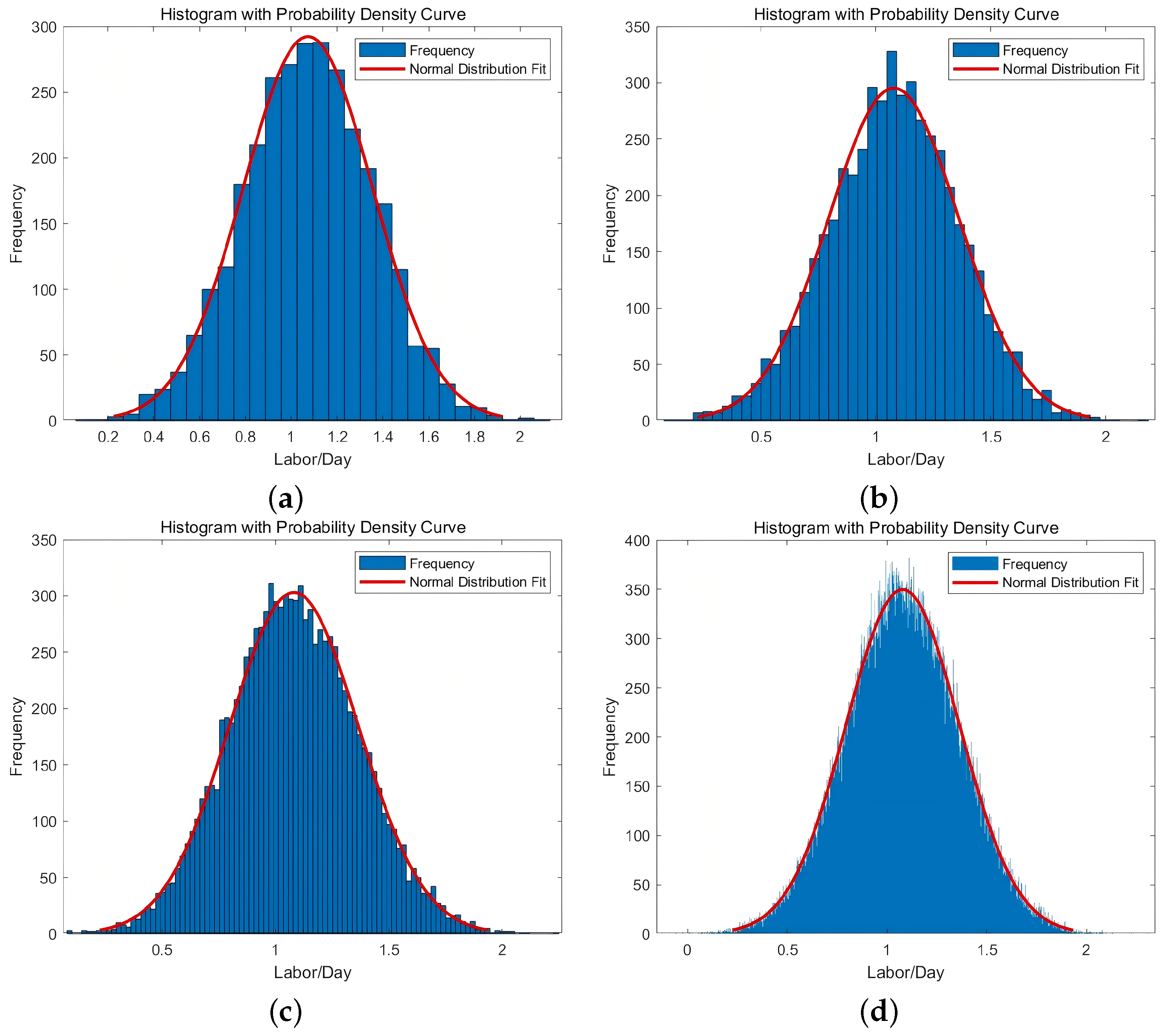
3.5. Results of Data Simulation and Distribution Analysis
3.6. Results of Resource Consumption Standard Determination
3.7. Results of Standard Validation
4. Conclusions
Author Contributions
Funding
Institutional Review Board Statement
Informed Consent Statement
Data Availability Statement
Conflicts of Interest
References
- Cao, S.; Xu, H.; Xu, Y.; Wang, X.; Zheng, Y.; Li, Y. Assessment of the integrated benefits of highway infrastructure and analysis of the spatiotemporal variation: Evidence from 29 provinces in China. Socio-Econ. Plan. Sci. 2023, 90, 101740. [Google Scholar] [CrossRef]
- Croce, A.I.; Musolino, G.; Rindone, C.; Vitetta, A. Traffic and Energy Consumption Modelling of Electric Vehicles: Parameter Updating from Floating and Probe Vehicle Data. Energies 2021, 15, 82. [Google Scholar] [CrossRef]
- Shi, R.; Gao, Y.; Ning, J.; Tang, K.; Jia, L. Research on Highway Self-Consistent Energy System Planning with Uncertain Wind and Photovoltaic Power Output. Sustainability 2023, 15, 3166. [Google Scholar] [CrossRef]
- Ishii, K. A production research to create new value of business output. Int. J. Prod. Res. 2013, 51, 7313–7328. [Google Scholar] [CrossRef]
- Aft, L. Work Measurement in the Computer Age. 2024. Available online: https://www.semanticscholar.org/paper/WORK-MEASUREMENT-IN-THE-COMPUTER-AGE-Aft/4b31df04dad492cdeec2c8af6382634dd5f0d389 (accessed on 24 September 2024).
- Uddin, N.; Hossain, F. Evolution of Modern Management through Taylorism: An Adjustment of Scientific Management Comprising Behavioral Science. Procedia Comput. Sci. 2015, 62, 578–584. [Google Scholar] [CrossRef]
- Vigoya, L.; Fernandez, D.; Carneiro, V.; Cacheda, F. Annotated Dataset for Anomaly Detection in a Data Center with IoT Sensors. Sensors 2020, 20, 3745. [Google Scholar] [CrossRef]
- Zhang, R.; Li, J.L. The application of activity-based costing in the cost calculation of thermal-power enterprise. Therm. Sci. 2021, 25, 933–939. [Google Scholar] [CrossRef]
- Homburg, C. A note on optimal cost driver selection in ABC. Manag. Account. Res. 2001, 12, 197–205. [Google Scholar] [CrossRef]
- Relph, G.; Barrar, P. Overage inventory—How does it occur and why is it important? Int. J. Prod. Econ. 2003, 81–82, 163–171. [Google Scholar] [CrossRef]
- Kim, Y.W.; Han, S.H.; Yi, J.S.; Chang, S. Supply chain cost model for prefabricated building material based on time-driven activity-based costing. Can. J. Civ. Eng. 2016, 43, 287–293. [Google Scholar] [CrossRef]
- Wang, C.; Mahmood, H.; Khalid, S. Examining the impact of globalization and natural resources on environmental sustainability in G20 countries. Sci. Rep. 2024, 14, 30921. [Google Scholar] [CrossRef] [PubMed]
- Proverbs, D.; Holt, G.; Olomolaiye, P. A method for estimating labour requirements and costs for international construction projects at inception. Build. Environ. 1998, 34, 43–48. [Google Scholar] [CrossRef]
- Wong, J.M.W.; Chan, A.P.C.; Chiang, Y.H. Modeling and Forecasting Construction Labor Demand: Multivariate Analysis. J. Constr. Eng. Manag. 2008, 134, 664–672. [Google Scholar] [CrossRef]
- Sing, C.p.; Love, P.E.D.; Tam, C.M. Multiplier Model for Forecasting Manpower Demand. J. Constr. Eng. Manag. 2012, 138, 1161–1168. [Google Scholar] [CrossRef]
- Peng, J.; Jiang, B.; Chen, H.; Liang, S.; Liang, H.; Li, S.; Han, J.; Liu, Q.; Cheng, J.; Yao, Y.; et al. A New Empirical Estimation Scheme for Daily Net Radiation at the Ocean Surface. Remote Sens. 2021, 13, 4170. [Google Scholar] [CrossRef]
- Guo, C.; Lu, M.; Wei, W. An improved LDA topic modeling method based on partition for medium and long texts. Ann. Data Sci. 2021, 8, 331–344. [Google Scholar] [CrossRef]
- Figuera, P.; García Bringas, P. Revisiting probabilistic latent semantic analysis: Extensions, challenges and insights. Technologies 2024, 12, 5. [Google Scholar] [CrossRef]
- Zhang, H.; Deng, J.; Xu, Y.; Deng, Y.; Lin, J.R. An Adaptive Pedestrian Flow Prediction Model Based on First-Order Differential Error Adjustment and Hidden Markov Model. Buildings 2025, 15, 902. [Google Scholar] [CrossRef]
- Wang, M.; Li, X.; Chen, L.; Chen, H.; Chen, C.; Liu, M. A deep-based Gaussian mixture model algorithm for large-scale many objective optimization. Appl. Soft Comput. 2025, 172, 112874. [Google Scholar] [CrossRef]
- Mahajan, A.; Das, S.; Su, W.; Bui, V.H. Bayesian-Neural-Network-Based Approach for Probabilistic Prediction of Building-Energy Demands. Sustainability 2024, 16, 9943. [Google Scholar] [CrossRef]
- Hasni, M.; Babai, M.; Aguir, M.; Jemai, Z. An investigation on bootstrapping forecasting methods for intermittent demands. Int. J. Prod. Econ. 2019, 209, 20–29. [Google Scholar] [CrossRef]
- Dao, D.V.; Adeli, H.; Ly, H.B.; Le, L.M.; Le, V.M.; Le, T.T.; Pham, B.T. A sensitivity and robustness analysis of GPR and ANN for high-performance concrete compressive strength prediction using a Monte Carlo simulation. Sustainability 2020, 12, 830. [Google Scholar] [CrossRef]
- Yang, C.; Kumar, M. On the effectiveness of Monte Carlo for initial uncertainty forecasting in nonlinear dynamical systems. Automatica 2018, 87, 301–309. [Google Scholar] [CrossRef]
- Tamang, N.; Sun, Y. Application of the dynamic Monte Carlo method to pedestrian evacuation dynamics. Appl. Math. Comput. 2023, 445, 127876. [Google Scholar] [CrossRef]
- Yu, S.; Wu, W.; Naess, A. Extreme value prediction with modified Enhanced Monte Carlo method based on tail index correction. J. Sea Res. 2023, 192, 102354. [Google Scholar] [CrossRef]
- Darmanto, T.; Tjen, J.; Hoendarto, G. Monte Carlo Simulation-Based Regression Tree Algorithm for Predicting Energy Consumption from Scarce Dataset. J. Data Sci. Intell. Syst. 2024, 1–9. [Google Scholar] [CrossRef]
- Maia, A.G.; Camargo-Valero, M.A.; Trigg, M.A.; Khan, A. Uncertainty and Sensitivity Analysis in Reservoir Modeling: A Monte Carlo Simulation Approach. Water Resour. Manag. 2024, 38, 2835–2850. [Google Scholar] [CrossRef]
- Mao, J.; Wang, H.; Li, J. Bayesian Finite Element Model Updating of a Long-Span Suspension Bridge Utilizing Hybrid Monte Carlo Simulation and Kriging Predictor. KSCE J. Civ. Eng. 2020, 24, 569–579. [Google Scholar] [CrossRef]
- Xiao, C.; Mei, J.; Müller, M. Memory-augmented Monte Carlo Tree Search. In Proceedings of the Thirty-Second AAAI Conference on Artificial Intelligence and Thirtieth Innovative Applications of Artificial Intelligence Conference and Eighth AAAI Symposium on Educational Advances in Artificial Intelligence, New Orleans, LA, USA, 2–7 February 2018; pp. 1455–1461. [Google Scholar]
- Xing, Y.; Li, F.; Sun, K.; Wang, D.; Chen, T.; Zhang, Z. Multi-type electric vehicle load prediction based on Monte Carlo simulation. Energy Rep. 2022, 8, 966–972. [Google Scholar] [CrossRef]
- Eraslan, E.; İundefined, Y.T. An improved decision support system for ABC inventory classification. Evol. Syst. 2019, 11, 683–696. [Google Scholar] [CrossRef]
- JTG/T 3832-2018; Highway Engineering Budget Standards. Ministry of Transport of the People’s Republic of China: Beijing, China, 2018.

| No. | Function Name | Probability Model | Characteristics |
|---|---|---|---|
| 1 | Uniform distribution | The probability is constant over the interval [a,b], indicating that any two values within the range have equal probability. It is suitable for variables with a known limited range or cases where the possible values are unclear. | |
| 2 | Normal distribution | Also called the Gaussian distribution, it forms a bell-shaped curve where the probability is higher in the middle and lower at both ends. This is a typical distribution pattern in natural phenomena. | |
| 3 | Triangular distribution | A continuous probability distribution resembling a triangular shape, increasing from the minimum to the maximum value and then decreasing. The peak determines the height of the triangle. | |
| 4 | Step distribution | Consists of several intervals, where the probability density remains constant within each interval but is zero elsewhere. |
| Item | Labor (Workdays) | Expansion Bolts (Sets) | Other Materials | 3t Electric Cart (Shift) | Small Tools |
|---|---|---|---|---|---|
| Manual barrier gate | 1.1 | 6.1 | 1.9 | 0.19 | 11.3 |
| Item | Labor | Expansion Bolts | Other Materials | 3t Electric Cart | Small Tools | Item | Labor | Expansion Bolts | Other Materials | 3t Electric Cart | Small Tools |
|---|---|---|---|---|---|---|---|---|---|---|---|
| 1 | 0.56 | 4.22 | 0.33 | 0.02 | 9.30 | 21 | 1.06 | 5.97 | 1.80 | 0.20 | 11.26 |
| 2 | 0.60 | 4.40 | 0.53 | 0.03 | 9.44 | 22 | 1.09 | 5.98 | 1.85 | 0.21 | 11.35 |
| 3 | 0.62 | 4.58 | 0.65 | 0.05 | 9.66 | 23 | 1.10 | 6.08 | 1.95 | 0.21 | 11.38 |
| 4 | 0.70 | 4.65 | 0.68 | 0.05 | 9.88 | 24 | 1.11 | 6.14 | 2.03 | 0.22 | 11.44 |
| 5 | 0.71 | 4.77 | 0.80 | 0.07 | 10.05 | 25 | 1.16 | 6.20 | 2.08 | 0.23 | 11.52 |
| 6 | 0.78 | 4.80 | 0.85 | 0.09 | 10.16 | 26 | 1.19 | 6.30 | 2.14 | 0.23 | 11.63 |
| 7 | 0.79 | 4.93 | 1.05 | 0.10 | 10.22 | 27 | 1.2 | 6.34 | 2.21 | 0.24 | 11.70 |
| 8 | 0.80 | 5.02 | 1.24 | 0.11 | 10.39 | 28 | 1.22 | 6.40 | 2.28 | 0.25 | 11.80 |
| 9 | 0.85 | 5.11 | 1.37 | 0.12 | 10.45 | 29 | 1.24 | 6.53 | 2.30 | 0.26 | 11.95 |
| 10 | 0.88 | 5.28 | 1.40 | 0.12 | 10.57 | 30 | 1.27 | 6.61 | 2.42 | 0.27 | 12.18 |
| 11 | 0.9 | 5.42 | 1.42 | 0.13 | 10.62 | 31 | 1.28 | 6.70 | 2.53 | 0.27 | 12.29 |
| 12 | 0.92 | 5.55 | 1.48 | 0.13 | 10.70 | 32 | 1.31 | 6.94 | 2.65 | 0.28 | 12.42 |
| 13 | 0.94 | 5.59 | 1.57 | 0.15 | 10.72 | 33 | 1.35 | 7.01 | 2.76 | 0.29 | 12.60 |
| 14 | 0.95 | 5.62 | 1.59 | 0.15 | 10.77 | 34 | 1.37 | 7.15 | 2.80 | 0.31 | 12.70 |
| 15 | 0.96 | 5.68 | 1.64 | 0.16 | 10.85 | 35 | 1.43 | 7.25 | 2.94 | 0.31 | 12.98 |
| 16 | 0.96 | 5.73 | 1.68 | 0.16 | 10.96 | 36 | 1.49 | 7.40 | 3.02 | 0.32 | 13.10 |
| 17 | 0.98 | 5.90 | 1.70 | 0.17 | 11.00 | 37 | 1.51 | 7.54 | 3.19 | 0.33 | 13.38 |
| 18 | 0.99 | 5.90 | 1.72 | 0.17 | 11.05 | 38 | 1.57 | 7.65 | 3.27 | 0.35 | 13.55 |
| 19 | 1.00 | 5.92 | 1.75 | 0.18 | 11.09 | 39 | 1.60 | 7.71 | 3.33 | 0.37 | 13.85 |
| 20 | 1.04 | 5.95 | 1.80 | 0.19 | 11.15 | 40 | 1.66 | 7.80 | 3.40 | 0.37 | 14.30 |
| Item | Labor | Expansion Bolts | Other Materials | 3t Electric Cart | Small Tools |
|---|---|---|---|---|---|
| Bessel’s Standard Deviation | 0.285 | 0.968 | 0.812 | 0.096 | 1.224 |
| Bessel’s standard deviation | 0.296 | 0.979 | 0.825 | 0.101 | 1.232 |
| 0.034 | 0.011 | 0.017 | 0.050 | 0.007 | |
| Systematic error judgment result | None | None | None | None | None |
| Upper Grubbs | 1.817 | 1.857 | 1.940 | 1.849 | 1.817 |
| Lower Grubbs | 1.967 | 1.821 | 1.811 | 1.723 | 1.967 |
| Grubbs’ threshold | 2.870 | 2.870 | 2.870 | 2.870 | 2.870 |
| Gross error detection | None | None | None | None | None |
| Maximum limit | 1.849 | 8.524 | 4.054 | 0.442 | 14.910 |
| Minimum limit | 0.309 | 3.512 | −0.244 | −0.048 | 7.910 |
| Outliers | None | None | None | None | None |
| Item | Labor | Expansion Bolts | Other Materials | 3t Electric Cart | Small Tools |
|---|---|---|---|---|---|
| Skewness coefficient | 0.054 | 0.098 | 0.052 | 0.002 | 0.590 |
| Kurtosis coefficient | 2.304 | 2.209 | 2.299 | 2.134 | 2.622 |
| Item | Labor | Expansion Bolts | Other Materials | 3t Electric Cart | Small Tools |
|---|---|---|---|---|---|
| Mean | 1.079 | 6.018 | 1.905 | 0.197 | 11.410 |
| Standard Deviation | 0.285 | 0.968 | 0.812 | 0.096 | 1.223 |
| 1.96 | 1.96 | 1.96 | 1.96 | 1.96 | |
| Minimum limit | 1.077 | 5.999 | 1.889 | 0.195 | 11.386 |
| Maximum limit | 1.081 | 6.037 | 0.016 | 0.199 | 11.434 |
| Absolute error | 0.019 | 0.015 | 0.024 | ||
| Relative error | |||||
| Accuracy compliance | Compliant | Compliant | Compliant | Compliant | Compliant |
| Item | National Standards | Budget Standards | Deviation (%) |
|---|---|---|---|
| Labor (workdays) | 1.1 | 1.111 | 1.03 |
| Expansion bolts (sets) | 6.1 | 6.199 | 1.62 |
| Other materials (CNY) | 1.9 | 1.962 | 3.27 |
| 3t electric cart (shift) | 0.19 | 0.203 | 6.79 |
| Small tools (CNY) | 11.3 | 11.752 | 4.00 |
| Price (CNY) | 205 | 200 | −2.44% |
| Item | National Standards (CNY) | Budget Standards (CNY) | Market Price (CNY) |
|---|---|---|---|
| Base price | 205 | 200 | 201.20 |
| Deviation (%) | −2.44 | - | −0.60 |
Disclaimer/Publisher’s Note: The statements, opinions and data contained in all publications are solely those of the individual author(s) and contributor(s) and not of MDPI and/or the editor(s). MDPI and/or the editor(s) disclaim responsibility for any injury to people or property resulting from any ideas, methods, instructions or products referred to in the content. |
© 2025 by the authors. Licensee MDPI, Basel, Switzerland. This article is an open access article distributed under the terms and conditions of the Creative Commons Attribution (CC BY) license (https://creativecommons.org/licenses/by/4.0/).
Share and Cite
Liu, L.; Tian, W.; Dai, X.; Song, L. Research on Resource Consumption Standards for Highway Electromechanical Equipment Based on Monte Carlo Model. Sustainability 2025, 17, 4640. https://doi.org/10.3390/su17104640
Liu L, Tian W, Dai X, Song L. Research on Resource Consumption Standards for Highway Electromechanical Equipment Based on Monte Carlo Model. Sustainability. 2025; 17(10):4640. https://doi.org/10.3390/su17104640
Chicago/Turabian StyleLiu, Linxuan, Wei Tian, Xiaomin Dai, and Liang Song. 2025. "Research on Resource Consumption Standards for Highway Electromechanical Equipment Based on Monte Carlo Model" Sustainability 17, no. 10: 4640. https://doi.org/10.3390/su17104640
APA StyleLiu, L., Tian, W., Dai, X., & Song, L. (2025). Research on Resource Consumption Standards for Highway Electromechanical Equipment Based on Monte Carlo Model. Sustainability, 17(10), 4640. https://doi.org/10.3390/su17104640