Do Non-Agricultural Sectors Affect Food Security in Saudi Arabia?

Abstract

Saudi Vision 2030 is a strategic goal that aims to diminish Saudi Arabia’s dependence on oil and diversify its economy, which requires considering the agricultural sector a target sector (among others). The agricultural sector represents the backbone of food security. This research aimed to assess the influence of the industrial sector, employment, and service sector on the agricultural sector in Saudi Arabia. Secondary data for the period from 1991 to 2022 were collected and analyzed using the ARDL model test, vector error correction, the Granger causality test, and multiple regression models. In addition, an impulse test was used to highlight the leading variables among all the variables under study, and quantitative analysis was performed to assess the impact of growth sectors on food security. The results point to the existence of long-term integration between the variables. Industrial and employment factors negatively affected food security (value-added agriculture), while the service sector had a positive effect. Based on the results of this study, the following recommendations were drawn: Policymakers should invest in technology and mechanization to fulfill labor requirements and enhance agricultural education and training. Integrated development plans should be adopted through design policies that combine agricultural and industrial growth, such as agro-processing industries, which add value to agricultural products. Dual-sector development strategies should be established to encourage exchange between sectors by fostering linkages, such as supplying industrial support for agricultural mechanization and irrigation.

1. Introduction

Food is a fundamental pillar upon which human life is built. Hence, the importance of agriculture cannot be overstated, as it serves as a primary source of food. Therefore, countries worldwide invest in the development of the agricultural sector through the expansion of agricultural areas, land reclamation, and the introduction of modern technology to achieve self-sufficiency, which in turn ensures food security and contributes significantly to the economy. Indeed, with rapid population growth and urban expansion worldwide, accompanied by an increase in needs, countries find themselves in urgent need of a greater increase in agricultural growth [1]. This is essential for setting developmental goals and plans in such countries [1].

The relationship between agricultural sectors and other economic sectors plays a vigorous role in the economic growth of various countries [2,3,4,5]. The agricultural sector is a key component in maintaining food security by supporting sustainable production, distribution, and access to food resources. Food security is defined as the availability and safety of food products, in addition to environment preservation [3,6]. This depends mainly on the positive impact achieved in combination with the growth of other economic sectors [3].

Regarding inter-linkages among dissimilar sectors of the economy, assumptions are chiefly grounded on the dual economic model [7] and on the concept of unbalanced growth development [8]. The authors of [7] described the inter-relationship between agricultural and industrial sectors and their contribution to economic growth.

Based on this notion, the agricultural sector is also considered crucial for developing countries progressing to the second stage (industrialization) through acquiring capital.

The route of converting an economy from the first stage (rural agricultural-sector-based) to the second stage (recent industrial-sector-based) must be established by balancing the development of whole economic sectors to achieve self-sustaining progress [7,8]. The theory of unbalanced growth discusses the necessity of capital to achieve high growth in developing countries, but such capital formation faces constraints [9]. The authors of [9] indicated that capital formation can be realized by sectors with the highest number of linkages that can encourage the development of production, employment, and income more rapidly. Consequently, the notion of unbalanced growth is similarly intertwined with inter-sectoral links.

2. Literature Review

Various economists have written about the relationship between the agricultural sector and other sectors of the economy. The following are some of them:

The authors of [10,11] examined the association between the agricultural and industrial sectors from different viewpoints, as follows: The agricultural sector supplies raw materials to the industrial sector, generates savings, affects private investors’ decisions due to its fluctuations [12], and affects the production of the industrial sector through purchaser demand. Meanwhile, the industrial sector provides agricultural inputs such as machinery, pipes, and chemical nutrients.

Some of these cross-sectoral relationships have already been formulated in [13,14,15]. Some channels emphasize supply-side linkages to meet their input needs, while others focus on demand-side linkages that arise from the interdependence between sectors to meet their final consumption demand.

Moreover, founded on the form of interconnection among sectors, the relations can also be separated into two types, as follows: a backward link, which involves the sector’s dependence on other sectors for input materials; and a forward link, which involves how the sector’s production is distributed among the remaining economic sectors.

In contrast to the interconnections between the agricultural and industrial sectors, the associations between the agricultural and service sectors are only one-way and primarily backward links, while the industry sector has dual forward and backward links with the service sector.

The authors of [16] reported that the service sector has considerably more robust backward links than forward links with both the agricultural and industrial sectors. The interconnections among these sectors influence the production of the agricultural sector, where the majority of the products contain foodstuff.

Therefore, these cross-sectoral links can similarly highlight the vital role of these sectors in long-term food availability.

After these interlinkages are recognized, the evidence can be used to conclude the goals of various policies implemented by a nation. For example, the existence of long-term stability among diverse sectors of the economy can influence some policy results.

For instance, the relationship between the agricultural and industrial sectors may be negative in the short term, while the relationship in the long term may be positive. This means that the impact of the growth of the industrial sector on the agricultural sector in the short term will be negative. However, the long-term impact will be positive. Consequently, understanding short-term and long-term interdependencies and their impacts can be useful in elucidating some policy results, as well as in finding the best policy for a country [17].

The agricultural sector is the oldest and most vital sector in the world. The world’s population is increasing speedily, increasing the demand for food and jobs [18]. During global crises, such as the COVID-19 pandemic, this sector is faced with a labor shortage. The COVID-19 pandemic has impacted the agricultural labor force, particularly seasonal agricultural laborers. These workers are often migrant workers, usually harvesting crops, and possess high physical and motor skills [19,20,21]. Lockdowns and limitations on cross-border labor movement have contributed to labor shortages, particularly in countries that depend on seasonal laborers [19].

The contributions of the agricultural, industrial, service, and labor sectors in the Saudi economy are as follows:

The agricultural sector: Saudi Arabia’s Vision 2030 focuses on local strategic aims, comprising economic growth and broadening the economy [22]. The author of [22] associated agricultural growth with achieving water and food security, in addition to environmental equilibrium. Therefore, food security is one of the goals of Vision 2030 [22]. Numerous plans have been developed, including growing production and marketing capability in the agricultural sector [23]. Notably, the Kingdom has realized self-sufficiency in dates and milk through concentrated agricultural production. Moreover, the self-sufficiency rates in the production of fruits, fish, and vegetables account for 60%, 59%, and 80%, respectively [24].

The industrial sector: Industrialization denotes the conversion of inputs into end products or services [25]. In Saudi Arabia, rapid industrialization has occurred in all sectors of the economy in the past few years. This mirrors the government’s approach regarding the development and enlargement of the economy. The Saudi government is dedicated to comprehensive growth, economic development, and the development of different industrial sectors to achieve a stable gross domestic product. The government launched the Saudi Industrial Development Fund and the National Industrial Development Logistics Program to support the multi-dimensional industrial sectors [25]. It stimulated industrial growth and encouraged all production sectors; therefore, the manufacturing sector has observed remarkable development over the last four decades. The Saudi government realized substantial development in the industrial sector, reaching SAR 32 billion in 1974 and increasing to about SAR 319.5 billion in 2018, supported by an adequate average growth rate of 5.2% annually [25]. The industrial sector’s contribution to GDP improved by 9% and reached 12% between 1974 and 2018 [25].

The authors of [26] investigated the role of the manufacturing sector in driving economic growth in the Saudi economy, using annual time series data from 1980 to 2018, which were collected from the Saudi Arabian Monetary Authority’s databases. Furthermore, the cointegration approach and the vector error correction model (VECM) were used to analyze both the short- and long-run causal relationships between the variables. The outcomes showed a bidirectional causal connection between the manufacturing sector and economic growth. Additionally, the outcomes showed that there is a unidirectional causal association running from the manufacturing sector to the service sector. This study recommended further research into the key factors driving growth in the Saudi manufacturing sector. It also emphasized the need to identify the most productive industries within this sector and enhance the productivity of other sectors in line with national economic plans and policies. Therefore, approving economic policies that encourage investment in the manufacturing sector will boost non-oil exports and contribute to diversifying sources of income, in line with the goals of Saudi Vision 2030.

The service sector: The service sector plays a vital role in the Saudi economy [22]. Vision 2030 focuses on tourism, finance, technology, and entertainment. Saudia Arabia is establishing a strong economy that offers long-term stability, growth, and prospects for its population.

The labor sector: The employment sector plays a vital role in the Saudi economy, as it drives the growth and innovation of key industries. The effects of the employment sector on the Saudi economy are categorized into several key areas, including the impact on GDP and productivity through job creation. Job creation increases employment across sectors and immediately improves GDP by increasing productivity and household spending.

This study aimed to examine the dynamics of the short- and long-term influences of inter-sectoral bonds between agricultural, industrial, service, and labor sectors and to determine the potential effects on food security in Saudia Arabia. This study supports policymakers in planning suitable policies regarding the linkages among various sectors of the economy and their impact on food security (food availability).

3. Materials and Methods

3.1. Description of Data

To highlight the relationship between the agricultural, industrial, service, and employment sectors, data were derived from 1991 to 2022 and are summarized in

Table 1. Data variables.

Variable	Unit	Sources
AG	USD million	https://databank.worldbank.org/reports.aspx?source=world-development-indicators# (accessed on 23 April 2024)
IN
SE
EM	1000 persons	https://www.fao.org/faostat/ar/#data/OEA (accessed on 23 April 2024)

AG—value-added agriculture, forestry, and fishing; IN—value-added industry; SE—value-added service; and Em—employment in agriculture, ILO estimates (1000 persons).

[27,28]. The data were analyzed using EViews 9.

3.2. Methods of Analysis

3.2.1. Descriptive and Graphic Analyses

Descriptive statistics and graphic analyses were conducted to examine data cointegration through a visual inspection.

3.2.2. Cointegration Tests: Investigating Long-Term Relationships

1. Unit root test: In terms of selecting proper techniques for the analysis of long-term relationships, the order of integration must be determined using the unit root test [29]. Regarding the following equations [30], an augmented Dickey–Fuller (ADF) test was used to investigate the integration order of the chain:

$$∆X_t=C_{t1}+B_1{X}_{t-1}+E_{t1}$$

(1)

$$∆X_t=C_{t2}+R_t+B_2{X}_{t-1}+E_{t2}$$

(2)

where B₁ and B₂ are ADF coefficients, R is the trend, C is a constant, and t is the time selected. In assessing H₀, X has a unit root, and, while against H₁, X is stationary. If the t-statistic of the ADF coefficient is greater than the critical t-values, it signifies that the variable is stationary. Additionally, the Phillips–Perron test was applied as the unit root test.

2. ARDL Bound Test: The ARDL model test was carried out to evaluate the long-term relationship between the series. Furthermore, this test outperforms other similar tests. It is efficient for small samples regardless of the order of the series I(0) and I(1) but not I(2). The following equations were used [31]:

$$∆X_t=C_1+{\sum }_{t-1}^p{a}_1∆Y_{t-1}+B_3{X}_{t-1}+B_4{Y}_{t-1}+e_1$$

(3)

$$∆Y_t=C_2+{\sum }_{t-1}^p{a}_2∆X_{t-1}+B_5{Y}_{t-1}+B_6{X}_{t-1}+e_2$$

(4)

ARDL is applied to investigate the presence of long-term linkage among the series. The acceptance of the null hypnosis illustrates no long-term relationship, where H0: b₃ = b₄ = 0 (Equation (3)) against the alternative hypothesis b₃ ≠ b₄ ≠ 0. Additionally, the same test was performed for the Y variable as an independent variable, where the null hypnosis b₅ = b₆ = 0 (Equation (4)) against the alternative hypothesis b₅ ≠ b₆ ≠ 0.

The authors of [32] applied the cumulative sum (CUSUM) technique to evaluate the stability of the ARDL model. If the residual is within the 5% critical threshold, it specifies that, at the 5% level of significance, the factors are constant.

Equations (3) and (4) include lower and upper bounds (two critical F-values) to evaluate whether the variables are integrated as order 1(0) and 1(1), respectively [31].

3.2.3. Error Correction Model (ECM)

If the cointegration test reveals a long-term correlation between the two variables, the ECM test is applied to estimate the velocity element of the short-run connection between the variables within the study period [33]. The ECM equations are as follows:

$$∆X_t={∆B}_7{X}_{t-1}+\sum _{t-1}^p{B}_8∆Y_{t-1}{+B}_9{U}_{t-1}+V$$

(5)

$$∆Y_t={∆B}_{10}{Y}_{t-1}+\sum _{t-1}^p{B}_{11}∆X_{t-1}{+B}_{12}{U}_{t-1}+V$$

(6)

where B₉ and B₁₂ denote the speeds of adjustment, which must be significant and negative to precisely model instability. The ECM viability was tested using residual diagnostic tests. The assessments were executed as follows:

Heteroskedasticity test (Breusch–Pagan–Godfrey): In this assessment, the null hypothesis is proved homoscedasticity, and the alternative hypothesis is proved heteroskedasticity. A p-value greater than 0.05 indicates failure to reject the null hypothesis, suggesting that the residuals are homoscedastic [8].

Residual normality is confirmed when the p-value of the Jarque–Bera statistic exceeds 0.05, indicating that the residuals follow normal distribution [8]. ]

Furthermore, impulse responses were assessed to measure the dynamic performance of vector autoregression (VAR) models and determine the model’s reaction to shock in one or more series [8,34].

3.2.4. Granger Causality Test

The Granger causality test was carried out using Equations (7) and (8) [35]:

$$X_t={\beta }_0+\sum _{j-1}^n{\beta }_{1j}{X}_{t-j}+\sum _{h-1}^m{\beta }_{2h}{Y}_{t-h}+e_{1t}$$

(7)

$$Y_t={\alpha }_0+\sum _{s-1}^k{\alpha }_{1s}{Y}_{t-s}+\sum _{i-1}^m{\alpha }_{2i}{X}_{t-m}+e_{2t}$$

(8)

In Equations (7) and (8), e_1t and e_2t are hypothetically not related, as e (ε_1t, ε_2t) = 0 = e (ε_2t, ε_2s) … s ≠ t. The following are the potential outcomes that can be extracted [2]:

-

If the coefficient β_2h ≠ 0 and is statistically significant, then Y→Granger causes→X [34,35];

-

If α₂ᵢ is significantly different from zero, this indicates that X exerts a statistically significant influence on Y [34,36,37];

-

The significance of α_2i and β_2h (≠0) is consistent with the joint dependence of X and Y;

-

If α_2i and β_2h are both equal to 0, then Y and X are independent.

3.2.5. Regression Analysis Method

To assess the impact of the industrial, service, and labor sectors (independent variables) on food security (agricultural sector as the dependent variable), regression analysis was performed. The CUSUM test was used to identify the stability of the cumulative sum of recursive residuals. The test revealed the stability of the parameter if the cumulative sum fell within the two critical thresholds, which indicates the consistency of the model. Consequently, the model was selected to estimate the influences of the independent variables (IN, SE, and EM) on AG. The following equation was used to obtain the results:

$$\mathrm{l}\mathrm{n}\mathrm{A}\mathrm{G}=\mathrm{c}+{\mathsf{\beta }}_1\mathrm{l}\mathrm{n}\mathrm{I}\mathrm{N}+{\mathsf{\beta }}_2\mathrm{l}\mathrm{n}\mathrm{S}\mathrm{E}+{\mathsf{\beta }}_3\mathrm{l}\mathrm{n}\mathrm{E}\mathrm{M}$$

(9)

where AG is the value-added agriculture (dependent variable), IN represents the value-added industry, SE signifies the value-added service, and EM denotes employment in agriculture (as independent variables), all of which were used to determine the coefficients.

3.2.6. The Impact of Industrial, Service, and Employment Sectors on Food Security: Qualitative Analysis

Built on the outcomes of different analyses (integration, causality, and regression), qualitative analyses were performed.

4. Results and Discussion

This study aimed to examine the dynamics of short- and long-term influences of inter-sectoral associations between agricultural, industrial, service, and labor sectors and to assess the potential impacts on food security in Saudia Arabia.

4.1. Descriptive Statistics and Graphic Results

Table 2. Descriptive statistical results.

	AG	IN	SE	EM
Mean	29,713	822,177	296,000.0	46,806
Median	16,853.0	776,000	281,000	33,000
Skewness	0.75	0.78	1.13	2.41
Kurtosis	2.35	3.37	4.80	10.12
Jarque–Bera	3.47	3.31	10.72	95.45
Probability	0.176	0.191	0.005	0.000
Observations	32	32	32	32

Source: Data were collected and analyzed.

records descriptive figure outcomes of the series. The probabilities of the Jarque–Bera figures were less than 0.05 for SE and EM, suggesting that the variables appeared to follow a non-normal distribution. Therefore, the data should be transformed (logarithm form) to correct for non-normal distribution.

Figure 1 illustrates the graphical analysis results of cointegration. The variables under study fluctuated together, indicating that the variables might be cointegrated.

4.2. Cointegration Test Analysis Results

4.2.1. Unit Root Tests Outcomes

Using a unit root test, the ADF statistics were detected as significant (1% level) at the first difference for the agricultural (AG), industrial (IN), and service sectors (SE), but not for the employment sector (EM) (

Table 3. Unit root test outcomes (at level).

Time Series	Intercept	Intercept and Trend	Stationarity	Intercept	Intercept and Trend	Stationarity
ADF				Phillips–Perron
LAG	2.06	−0.41	Non-Stationary	2.06	−0.41	Non-Stationary
LIN	−0.59	−2.08	Non-Stationary	−0.43	−2.20	Non-Stationary
LSE	−0.49	−3.12	Non-Stationary	0.28	−2.23	Non-Stationary
LEM	−4.22 *	−1.80	Stationary 1(0)	−2.90 **	5.82 *	Stationary 1(0)

Source: Data were collected and analyzed. * and ** at the 1% and 5% level of significance, respectively.

and

Table 4. Unit root test outcomes (at the first difference).

Time Series	Intercept	Intercept and Trend	Stationarity	Intercept	Intercept and Trend	Stationarity
ADF				Phillips–Perron
LAG	−2.82 ***	−3.51 ***	Stationary	−2.82 ***	−3.31 ***	Stationary
LIN	−4.75 *	−4.80 *	Non-stationary	−4.65 *	−4.51 *	Stationary
LSE	−3.13 **	−2.94	Non-stationary	−3.11 **	−2.91	Stationary

Source: Data were collected and analyzed. *, **, and *** at the 1%, 5%, and 10% level of significance, respectively.

). Hence, the AG, IN, and SE series were stationary at 1(1), while the EM series was at 1(0). Therefore, the ARDL bound test was elected to determine the link among the chains.

4.2.2. ARDL Tests Results

Table 5. ARDL tests results.

Model
LAG (Dependent Variable): Selected ARDL Model (1, 3, 1, 4)
Independent V.	Coefficient	t-Statistic	Prob.
LAG (-1)	0.440	3.17	0.006
LIN	−0.008	−0.49	0.630
LIN (-1)	−0.108	−5.54	0.000
LIN (-2)	0.013	0.56	0.581
LIN (-3)	0.053	−2.82	0.013
LSE	0.339	3.11	0.007
LSE (-1)	0.152	1.06	0.309
LEM	0.106	2.75	0.015
LEM (-1)	−0.130	−2.93	0.010
LEM (-2)	0.097	2.05	0.058
LEM (-3)	0.078	1.81	0.090
LEM (-4)	−0.310	−7.54	0.000
C	2.958	3.885602	0.0015
R-squared 0.9995		F-statistics 2371.54 Prob. 0.000
Adj. R-squared 0.9990		Durbin–Watson stat: 2.37

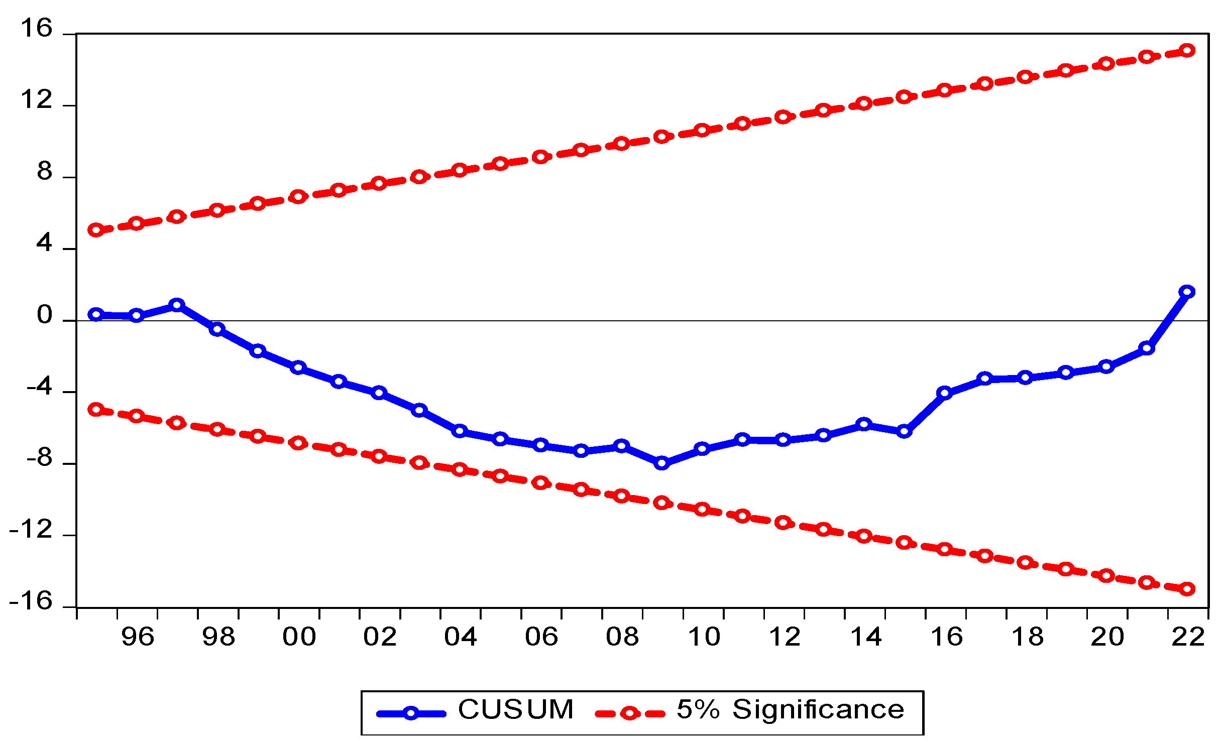
Source: Data were collected and analyzed. Figures in () are probabilities.

records the outcomes of the ARDL tests. The Jarque–Berat, Breusch–Pagan–Godfrey heteroskedasticity, and serial correlation LM (Breusch–Godfrey) tests were applied to reveal the ARDL model’s suitability for residual diagnostics (

Table 6. ARDL model diagnostic tests.

Test Statistics	Results
Serial Correlation LM Test: Breusch–Godfrey	3.78 (0.14)
Breusch–Pagan–Godfrey Heteroskedasticity Test	4.28 (0.97)
Jarque–Bera test	0.66 (0.72)

Source: Data were collected and analyzed.

). The data appeared to follow normal distribution, and the outcomes did not illustrate heteroskedasticity and serial correlation. Additionally, a CUSUM test was used to test diagnosis stability [38]. Since the CUSUM (blue color) is within the control bounds, the diagnosis is statistically stable over the tested period. The results highlight the stability of the cumulative sum of the recursive residuals, signifying the power of the model (Figure 2).

The bound test results were obtained from the ARDL model (

Table 7. Results of the bound test: ARDL (LAG as dependent variable).

Dependent	Function			F-Statistic
LAG	LAG = f (LIN, LSE, and LEM)			22.90
Significance:	10%	1%	5%
Lower Bound:	2.37	3.65	2.79
Upper Bound:	3.20	4.66	3.67

Source: Data were collected and analyzed.

). The bounds were used in the F-test for the AG coefficients (one lag period and dependent variables). The F-statistic was 22.9 for the model, which is higher than that of the upper bound of the bound critical F-statistic (4.66) at 1%, demonstrating a long-term relationship between the agricultural sector and the other variables (the industrial, service, and labor sectors). This outcome coincides with that of a preceding study [3]. The study outcomes show that there is a long-term association among the agricultural, industrial, and service sector outputs in Pakistan.

4.3. ECM Results

In order to apply the ECM, the lag must be known (

Table 8. Lag selection.

Lag	LogL	LR	FPE	AIC	SC	HQ
0	39.46	NA	1.11 × 10−6	−2.36	−2.18	−2.30
1	196.48	261.71 *	9.25 × 10−11 *	−11.77 *	−10.83 *	−11.47 *
2	205.8736	13.15	1.53 × 10−10	−11.33	−9.64	−10.79

Source: Data were collected and analyzed. * Denotes the lag order elected with the criterion. FPE: final prediction error; AIC: Akaike information criterion; HQ: Hannan–Quinn information criterion; LR: sequentially modified LR test statistic (each test at 5% level); SC: Schwarz information criterion.

). Lag 1 is indicated in Table 8. To reinforce the outcomes of a long-term association among the variables under study, which were determined using the ARDL test, the ECM was performed (

Table 9. Results of ECM test.

Long-Term Results: LAG (Dependent Variable)			Short-Term Results: LAG (Dependent Variable)
Error Correction	Coefficient	t-Value Statistic	Coefficient	t-Value Statistic
CointEq1	−0.004	−0.43
LIN (-1)	−3.24	−4.44
LSE (-1)	2.80	4.34
LEM (-1)	−1.16	−1.02
D(LAG (-1))			0.33	1.48
D(LIN (-1))			−0.06	−1.86
D(LSE (-1))			0.16	0.91
D(LEM (-1))			−013	−1.67
C	8.97		0.022	1.60
ECM residual serial correlation LM tests:		Lags	LM-Stat	Prob.
		1	10.23	0.85
VEC Residual Heteroskedasticity Tests:		Chi-sq: 109.50	Prob.: 0.24
VEC Residual Normality Tests:		Chi-sq: 109.50	Prob.:0.24

Source: Data were collected and analyzed.

). The adjustment parameter coefficient for the service sector (AG) (as a dependent variable) was found to be negative (−0.004) and insignificant (critical t-value = −0.43), concluding that the model was powerless to make precise its previous imbalance. Additionally, the outcomes propose that the adjustment parameter coefficients for the other variables (dependent variables) were statistically insignificant, signifying that the model may need more than one year to correct its preceding time imbalance. The long- and short-term results shown in the table indicate that the industrial sector influences agricultural value addition negatively. The negative relation in the short term may be due to labor moving from the agricultural sector to the industrial sector, while, in the long term, the negative relationship may be due to industrial growth, which leads to urbanization. Urbanization may decrease the accessibility of agricultural land and labor, leading to a reduction in agricultural value addition. These contrasting results are in agreement with a previous study’s results on the short- and long-term impact, respectively [3]. The study showed that the industrial sector affects the production of agricultural output negatively and positively in the long and short-term, respectively. Additionally, the results showed that employment negatively affects agricultural value addition in the short term, concluding that workers may be less efficient and transferring their labor to industry. The negative relationship between agricultural employment and added value may be due to the following: Low labor productivity is a key factor—agricultural employment in Saudi Arabia is largely characterized by low-skilled, seasonal, or migrant labor, with limited access to modern technology and training and institutional and structural inefficiencies, such as fragmented landholdings and water scarcity, which may further limit the productive capacity of labor. This result (less efficient labor in agriculture) may be due to the insufficient use of modern equipment and technology and untrained labor. In addition, the service sector positively influences agricultural value addition in the long term. This result may reflect the growth in the service sector, which implies improvement in transportation, communication, energy infrastructure, insurance, and financial services. These expansions allow farmers to access markets, decrease post-harvest losses, and efficiently transport goods, which boosts agricultural value addition. This result is in contrast to that of a previous study [3]. The authors of [3] found that the service sector influences the output of the agricultural sector negatively. To verify the VECM’s adequacy, the serial correlation of the residual LM and residual heteroskedasticity tests was investigated. The LM’s statistic (lag 1) was 10.23 with Prob. = 0.85, demonstrating no serial correlation. The Chi-square value was 109.5 with Prob. = 0.24, which does not indicate heteroskedasticity. The results of model adequacy tests confirmed the null hypothesis, no serial correlation of residuals, and no heteroskedasticity. The normality test indicated normal data distribution.

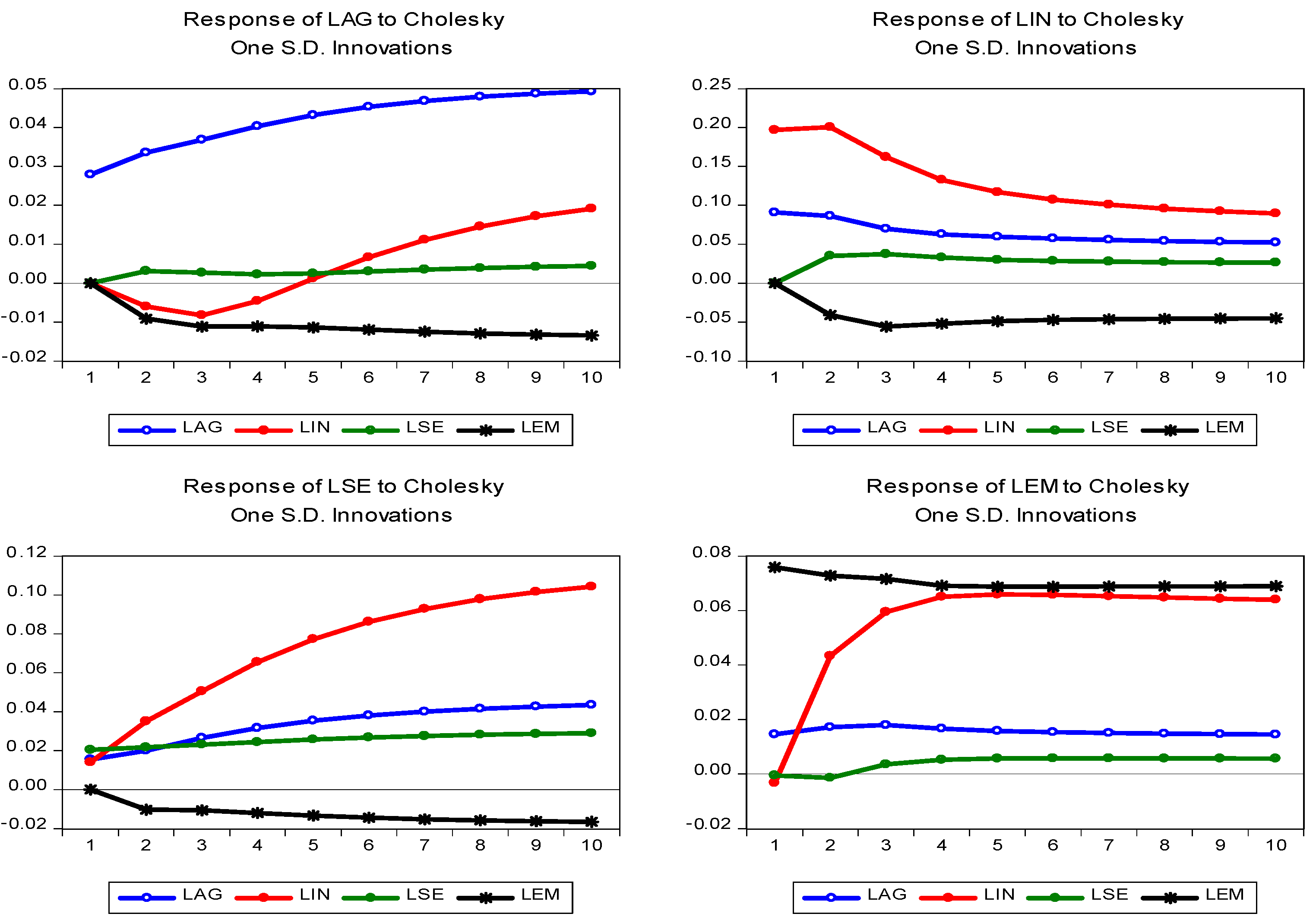
Additionally, an impulse test was used to determine the leading series that considerably impacts the other series in the long term (Figure 3). The responses of variables to the Cholesky one standard deviation innovation are shown in the figure (impulse responses), where the agricultural sector reveals a positive response in the long term compared to the other variables, indicating that it may reflect the chief variable. This outcome matches with the theoretical results of previous studies [39].

4.4. The Granger Causality Test Results

The F-statistics of the Granger causality test were 4.87 (probability, 0.036) and 6.22 (probability, 0.019) (

Table 10. Granger causality test results.

Null Hypothesis	F-Statistic	Prob.
LIN - LAG	1.35	0.256
LAG - LIN	0.88	0.356
LSE - LAG	4.87	0.036
LAG - LSE	6.22	0.019
LEM - LAG	0.52	0.476
LAG - LEM	1.09	0.307
LSE - LIN	0.88	0.357
LIN - LSE	31.34	5 × 10−6
LEM - LIN	0.57	0.456
LIN - LEM	0.92	0.345
LEM - LSE	10.04	0.004
LSE - LEM	0.72	0.403

Source: Data were collected and analyzed. - = is not Granger causality.

), indicating the presence of bidirectional causality between the agricultural sector and the service sector. Regarding the casualty from the service sector to the agricultural sector, this result agrees with a former study [40]. Additionally, unidirectional causality was observed from the labor and industrial sectors to the service sector, which is in contrast to a prior study [40].

4.5. Regression Analysis Results

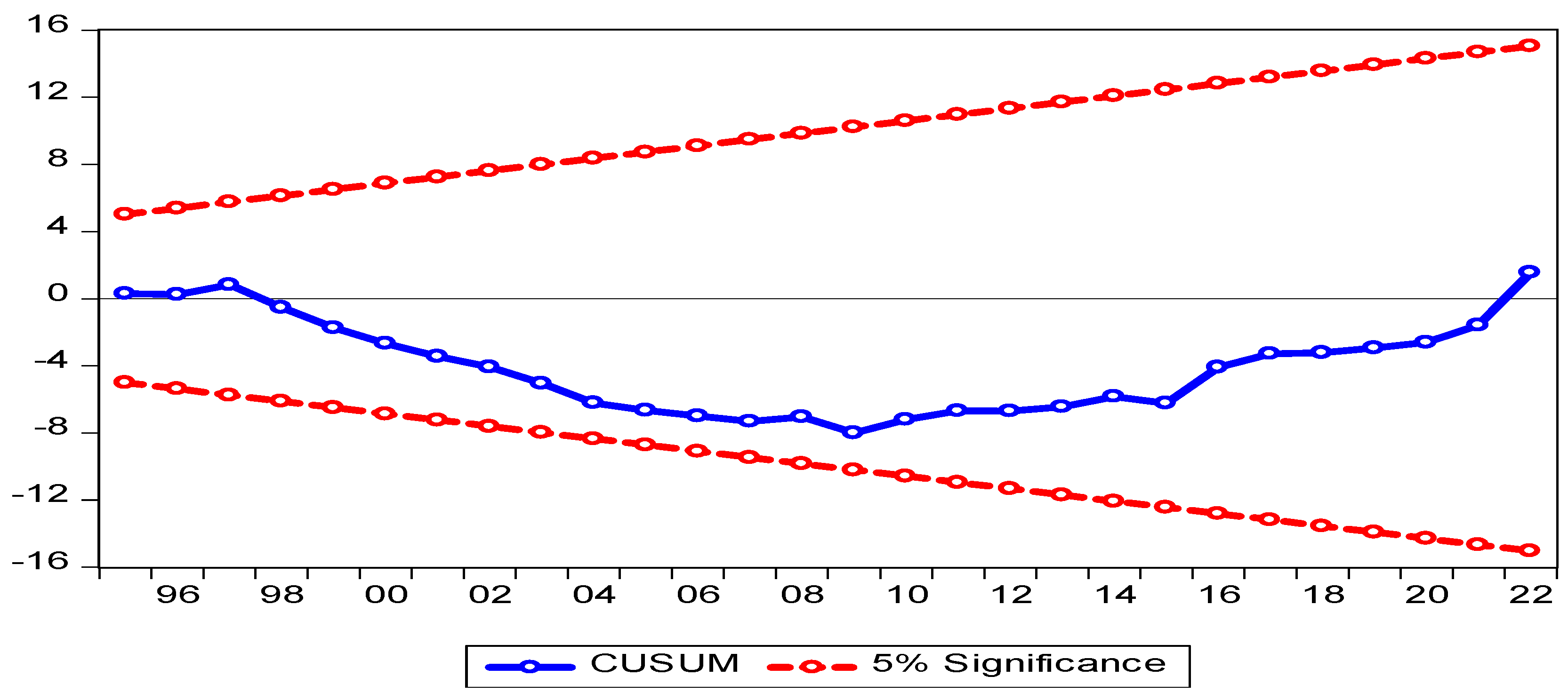
The regression analysis outcomes are presented in

Table 11. Regression analysis results (lnAG is the dependent variable).

Variable	Coefficient	t-Statistic	Prob.
LIN	−0.03	−0.85	0.4017
LSE	0.59	18.61	0.0000
LEM	−0.28	−4.52	0.0001
C	5.78	10.46	0.0000
R-squared = 0.988    Adjusted R-squared = 0.987 F-statistic = 761.412  Prob. (F-statistic) = 0.0000 Heteroskedasticity Test (Breusch–Pagan–Godfrey): 1.337 Prob = 0.28 LM-statistics (Breusch–Godfrey serial correlation of residual) F = 2.75 with Prob. = 0.08

Source: Author’s calculations based on collected data.

. Different scenarios were used to select a stable model. The results show that there is no autocorrelation among the consecutive values of the disturbance term, and the variance of the disturbance remains constant, indicating homoscedasticity. To assess model stability, the CUSUM test was conducted to determine the stability of the cumulative sum of the recursive residuals (Figure 4). Consequently, a regression model was selected and adopted to estimate the influences of the industrial, service, and labor sectors (independent variables) on the agricultural sector. In the table, the R-squared value indicates that 99% of the variations in the agricultural sector are interpreted through other sectors (independent variables). In addition, the F-statistic values show that the model is highly significant. The coefficients for the services sector (the independent variable) are positive and highly statistically significant, signifying strong explanatory power for changeability in the agricultural sector. Also, the labor sector appears to impact the agricultural sector negatively, with high significance. This result may be due to the presence of unskilled labor in the agricultural sector.

In Equation (10), increasing the SE and EM by 1% will increase and decrease AG by 0.59% and 0.28%, respectively. The equation used for estimation is as follows:

$$\mathrm{l}\mathrm{n}\mathrm{A}\mathrm{G}=5.78-0.03\mathrm{l}\mathrm{n}\mathrm{I}\mathrm{N}+0.59\mathrm{l}\mathrm{n}\mathrm{S}\mathrm{E}-0.28\mathrm{l}\mathrm{n}\mathrm{E}$$

(10)

4.6. The Impact of Growth Sectors on Food Security

Food security is delineated as “existing when all people, at all times, have physical and economic access to sufficient, safe, and nutritious food that meets their dietary needs and food preferences for an active and healthy life” [3,41,42]. This definition presents a broad concept of food security, encompassing four pillars, namely availability, access, utilization, and stability [42,43,44,45]. These pillars are interconnected with agricultural innovation [42,46], social capital [42,47], kitchen equipment [42,48], and worldwide shocks [42,49]. One of the fundamental pillars of food security is food availability, which refers to the consistent availability of sufficient quantities of food [50], directly derived from agriculture [51]. The agricultural sector plays a strategic role in improving food availability and achieving food security [52,53,54]. This study aimed to disclose the impacts of industry, services, and employment on food security (value-added agriculture). The long- and short-term results of the cointegration test revealed that the industrial sector influences agricultural production and value addition negatively, leading to worse food security. Additionally, the results show that employment negatively affects agricultural value addition in the short term, which may lead to a decline in food security. By contrast, the service sector positively influences agricultural value addition in the long term, improving food security. Regarding the regression analysis outcomes, the coefficients of the service sector (independent variable) positively and greatly significantly explained the variability in agricultural value addition, while the labor sector influenced agricultural value addition negatively.

5. Conclusions

Saudi Vision 2030 is a strategic goal that aims to diminish Saudi Arabia’s dependence on oil and diversify its economy, which involves considering the agricultural sector as a target sector (among others). The agricultural sector represents a pillar for achieving food security. This research evaluated the relationship and influence of the industrial sector, employment, and service sector on food security (agricultural sector) in Saudi Arabia. With secondary data from 1991 to 2022, the ARDL model test, vector error correction, the Granger causality test, multiple regression models, and an impulse test were used to highlight the leading variables among all of the variables under study. In addition, quantitative analysis was applied to test the impact of growth sectors on food security. The results reveal long-term integration between the variables. Industry and employment influence food security (value-added agriculture) negatively, whereas the service sector affects food security positively. This research contributes to achieving sustainability by examining the impact of the industrial, service, and employment sectors on food security in the Kingdom of Saudi Arabia. By identifying the impact of these sectors on food availability (food security), the findings support the Saudi Vision 2030 strategy, which directs the Kingdom toward a more diversified and resilient economy. Furthermore, this study contributes to achieving several of the United Nations Sustainable Development Goals, particularly the following: Goal 2: End hunger, achieve food security, and promote sustainable agriculture; Goal 8: Promote sustained, inclusive, and sustainable economic growth and full and productive employment; and Goal 9: Build resilient infrastructure and promote inclusive and sustainable industrialization. Overall, this research emphasizes the importance of sectoral integration in policy planning to ensure food security and sustainability. Based on the results, this study recommends the following, including Saudi Arabia’s national context and Vision 2030 objectives: Targeted training programs to upskill agricultural workers, incentives for capital investment in labor-saving technologies, and support for agribusiness value chains that integrate production with processing and marketing, particularly in regions with high unemployment. Policymakers should invest in technology and mechanization to fulfill labor requirements and enhance agricultural education and training. Integrated development plans should be adopted through design policies that integrate agricultural and industrial growth, such as agro-processing industries, which add value to agricultural products. Dual-sector development strategies should be established to encourage exchange between sectors by fostering linkages, for instance, by providing industrial support for agricultural mechanization and irrigation.

References

1. Kubiszewski, I.; Costanza, R.; Franco, C.; Lawn, P.; Talberth, J.; Jackson, T.; Aylmer, C. Beyond GDP: Measuring and achieving global genuine progress. Ecol. Econ. 2013, 93, 57–68. [Google Scholar] [CrossRef]
2. Emam, A. Saudi Fertilizers and Their Impact on Global Food Security: Present and Future. Sustainability 2023, 15, 7614. [Google Scholar] [CrossRef]
3. Asim, H.; Akbar, M. Sectoral growth linkages of agricultural sector: Implications for food security in Pakistan. Agric. Econ./Zeměd. Ekon. 2019, 65, 278–288. [Google Scholar] [CrossRef]
4. Singariya, M.R.; Naval, S.C. An empirical study of intersectoral linkages and economic growth in India. Am. J. Rural Dev. 2016, 4, 78–84. [Google Scholar] [CrossRef]
5. Johnston, B.F. Agriculture and structural transformation in developing countries: A survey of research. J. Econ. Lit. 1970, 8, 369–404. [Google Scholar]
6. Rehman, A.; Jingdong, L.; Iqbal, M.S.; Hussain, I. A study on agricultural development in China and its comparison with India and Pakistan. Transylv. Rev. 2016, 6, 603–610. [Google Scholar]
7. Lewis, W.A. Economic development with unlimited supplies of labour. Manch. Sch. 1954, 28, 139–191. [Google Scholar] [CrossRef]
8. Emam, A.A. Present and Future: Does agriculture affect economic growth and environment in the Kingdom of Saudi Arabia? J. Agric. Econ.-Czech Acad. Agric. Sci. 2022, 68, 361–370. [Google Scholar] [CrossRef]
9. Hirschman, A.O. The Strategy of Economic Development; Yale University Press: New Haven, CT, USA, 1958; pp. 41–97. [Google Scholar]
10. Thirlwall, A.P. The terms of trade, debt and development: With particular reference to Africa. Afr. Dev. Rev. 1995, 7, 1–34. [Google Scholar] [CrossRef]
11. Saikia, D. Analyzing inter-sectoral linkages in India. Afr. J. Agric. Res. 2011, 6, 6766–6775. [Google Scholar] [CrossRef]
12. Rangarajan, C. Agricultural Growth and Industrial Performance in India; International Food Policy Research Institute: Washington, DC, USA, 1982. [Google Scholar]
13. Feder, G. On exports and economic growth. J. Dev. Econ. 1983, 12, 59–73. [Google Scholar] [CrossRef]
14. Feder, G. Growth in semi-industrial countries: A statistical analysis. In Industrialization and Growth: A Comparative Study; Oxford University Press: New York, NY, USA, 1986; pp. 263–282. Available online: https://cir.nii.ac.jp/crid/1570572699882825088 (accessed on 14 January 2025).
15. Dowrick, S.J.; Gemmell, N. Industrialization, catching-up and economic growth: A comparative study across the world’s capitalist economies. Econ. J. 1991, 101, 263–275. [Google Scholar] [CrossRef]
16. Singh, N. Services-Led Industrialization in India: Assessment and Lessons. Department of Economics, UC Santa Cruz, Santa Cruz, CA, USA, 2006; p. 1. Available online: https://escholarship.org/uc/item/8jn2b8z6 (accessed on 15 January 2025).
17. Gemmell, N.; Lloyd, T.A.; Mathew, M. Agricultural growth and inter-sectoral linkages in a developing economy. J. Agric. Econ. 2000, 51, 353–370. [Google Scholar] [CrossRef]
18. Javaid, M.; Haleem, A.; Khan, I.H.; Suman, R. Understanding the potential applications of Artificial Intelligence in Agriculture Sector. Adv. Agrochem 2023, 2, 15–30. [Google Scholar] [CrossRef]
19. Bochtis, D.; Benos, L.; Lampridi, M.; Marinoudi, V.; Pearson, S.; Sørensen, C.G. Agricultural workforce crisis in light of the COVID-19 pandemic. Sustainability 2020, 12, 8212. [Google Scholar] [CrossRef]
20. Benos, L.; Tsaopoulos, D.; Bochtis, D. A review on ergonomics in agriculture. Part I: Manual operations. Appl. Sci. 2020, 10, 1905. [Google Scholar] [CrossRef]
21. Benos, L.; Tsaopoulos, D.; Bochtis, D. A review on ergonomics in agriculture. part II: Mechanized operations. Appl. Sci. 2020, 10, 3484. [Google Scholar] [CrossRef]
22. KSA Vision 2030. Strategic Objectives and Vision Realization Programs, Saudi Vision 2030. 2019. Available online: https://www.my.gov.sa/wps/portal/snp/content/saudivision/?lang=en (accessed on 10 October 2024).
23. Ministry of Environment, Water, and Agriculture. Annual Report of the Ministry of Agriculture. 2021. Available online: https://www.mewa.gov.sa/ar/InformationCenter/DocsCenter/YearlyReport/YearlyReports/%d8%a7%d9%84%d8%aa%d9%82%d8%b1%d9%8a%d8%b1%20%d8%a7%d9%84%d8%b3%d9%86%d9%88%d9%8a%20%d9%84%d9%84%d9%88%d8%b2%d8%a7%d8%b1%d8%a9%20%d9%84%d8%b9%d8%a7%d9%85%202021%d9%85.pdf (accessed on 13 December 2024).
24. FAO. Crops and Livestock Products. [Dataset]. Food and Agriculture Organization of the Nations (FAO). 2014. Available online: https://www.fao.org/faostat/en/#data/QCL (accessed on 2 January 2025).
25. Ali, A. Industrial Development in Saudi Arabia: Disparity in Growth and Development. Probl. Perspect. Manag. 2020, 18, 23–35. [Google Scholar] [CrossRef]
26. Sallam, M. The role of the manufacturing sector in promoting economic growth in the Saudi economy: A cointegration and VECM approach. J. Asian Financ. Econ. Bus. 2021, 8, 21–30. [Google Scholar] [CrossRef]
27. FAO. 2022. Available online: https://www.fao.org/faostat/ar/#data/OEA (accessed on 23 April 2024).
28. World Bank. 2022. Available online: https://databank.worldbank.org/reports.aspx?source=world-development-indicators# (accessed on 23 April 2024).
29. Emam, A.A. The Impacts of COVID-19: An Econometric Analysis of Crude Oil Prices and Rice Prices in the World. J. Agric. Sci. 2020, 35, 137–143. [Google Scholar] [CrossRef]
30. Dickey, D.A.; Fuller, W.A. Distribution of the estimators for autoregressive time series with a unit root. J. Am. Stat. Assoc. 1979, 74, 427–431. [Google Scholar] [CrossRef]
31. Pesaran, M.H.; Shin, Y.; Smith, R.J. Bounds testing approaches to the analysis of level relationships. J. Appl. Econom. 2001, 16, 289–326. [Google Scholar] [CrossRef]
32. Pesaran, M.H.; Pesaran, B. Working with Microfit 4.0: Interactive Econometric Analysis; Oxford University Press: Oxford, UK, 1997; Available online: https://cir.nii.ac.jp/crid/1130282270030044416 (accessed on 15 January 2025).
33. Venujayakanth, B.; Dudhat, A.S.; Swaminathan, B.; Ardeshana, N.J. Price integration analysis of major groundnut domestic markets in India. Econ. Aff. 2017, 62, 233–241. [Google Scholar] [CrossRef]
34. Lütkepohl, H. Impulse response function. In Macroeconometrics and Time Series Analysis; Durlauf, S.N., Blume, L.E., Eds.; The New Palgrave Economics Collection; Palgrave Macmillan: London, UK, 2010. [Google Scholar] [CrossRef]
35. Ivascu, L.; Sarfraz, M.; Mohsin, M.; Naseem, S.; Ozturk, I. The causes of occupational accidents and injuries in Romanian firms: An application of the Johansen cointegration and Granger causality test. Int. J. Environ. Res. Public Health 2021, 18, 7634. [Google Scholar] [CrossRef] [PubMed]
36. Belloumi, M. Energy consumption and GDP in Tunisia: Cointegration and causality analysis. Energy Policy 2009, 37, 2745–2753. [Google Scholar] [CrossRef]
37. Mohsin, M.; Naiwen, L.; Zia-UR-Rehman, M.; Naseem, S.; Baig, S.A. The volatility of bank stock prices and macroeconomic fundamentals in the Pakistani context: An application of GARCH and EGARCH models. Oeconomia Copernic. 2020, 11, 609–636. [Google Scholar] [CrossRef]
38. Ali, M.B. Co integrating relation between macroeconomic variables and stock return: Evidence from Dhaka Stock Exchange (DSE). IJESPG (Int. J. Eng. Econ. Soc. Politic Gov.) 2023, 1, 1–14. [Google Scholar] [CrossRef]
39. Zhai, X.; Geng, Z.; Zhang, X. Two-stage dynamic test of the determinants of the long-run decline of China’s monetary velocity. Chin. Econ. 2013, 46, 23–40. [Google Scholar] [CrossRef]
40. Kafando, N.C. Does the Development of the Agricultural Sector Affect the Manufacturing Sector. In Building a Resilient and Sustainable Agriculture in Sub-Saharan Africa; Shimeles, A., Verdier-Chouchane, A., Boly, A., Eds.; Palgrave Macmillan: Cham, Switzerland, 2018. [Google Scholar] [CrossRef]
41. Uddin, M.M.M. Causal relationship between agriculture, industry and services sector for GDP growth in Bangladesh: An econometric investigation. J. Poverty Investig. Dev. 2015, 8, 124–129. [Google Scholar]
42. World Food Summit. Declaration on World Food Security; World Food Summit: Rome, Italy, 1996. [Google Scholar]
43. Van Meijl, H.; Shutes, L.; Valin, H.; Stehfest, E.; van Dijk, M.; Kuiper, M.; Tabeau, A.; van Zeist, W.J.; Hasegawa, T.; Havlik, P. Modelling alternative futures of global food security: Insights from FOODSECURE. Glob. Food Secur. 2020, 25, 100358. [Google Scholar] [CrossRef]
44. FAO. The State of Food and Agriculture. 1996. Available online: http://www.fao.org/3/w1358e/w1358e00.htm (accessed on 14 January 2023).
45. Guiné, R.D.P.F.; Pato, M.L.D.J.; Costa, C.A.D.; Costa, D.D.V.T.A.D.; Silva, P.B.C.D.; Martinho, V.J.P.D. Food Security and Sustainability: Discussing the Four Pillars to Encompass Other Dimensions. Foods 2021, 10, 2732. [Google Scholar] [CrossRef]
46. Béné, C. Resilience of local food systems and links to food security—A review of some important concepts in the context of COVID-19 and other shocks. Food Secur. 2020, 12, 805–822. [Google Scholar] [CrossRef]
47. Magrini, E.; Vigani, M. Technology adoption and the multiple dimensions of food security: The case of maize in Tanzania. Food Secur. 2016, 8, 707–726. [Google Scholar] [CrossRef]
48. Nosratabadi, S.; Khazami, N.; Abdallah, M.B.; Lackner, Z.S.; Band, S.; Mosavi, A.; Mako, C. Social capital contributions to food security: A comprehensive literature review. Foods 2020, 9, 1650. [Google Scholar] [CrossRef]
49. Oakley, A.R.; Nikolaus, C.J.; Ellison, B.; Nickols-Richardson, S.M. Food insecurity and food preparation equipment in US households: Exploratory results from a cross-sectional questionnaire. J. Hum. Nutr. Diet. 2019, 32, 143–151. [Google Scholar] [CrossRef] [PubMed]
50. Houessou, M.D.; Cassee, A.; Sonneveld, B.G. The effects of the COVID-19 pandemic on food security in rural and urban settlements in benin: Do allotment gardens soften the blow? Sustainability 2021, 13, 7313. [Google Scholar] [CrossRef]
51. Ahmad, N.; Du, L.; Lu, J.; Wang, J.; Li, H.Z.; Hashmi, M.Z. Modelling the CO2 emissions and economic growth in Croatia: Is there any environmental Kuznets curve? Energy 2017, 123, 164–172. [Google Scholar] [CrossRef]
52. Smutka, L.; Steininger, M.; Miffek, O. World agricultural production and consumption. Agris-Line Pap. Econ. Inform. 2009, 1, 3–12. [Google Scholar] [CrossRef]
53. Otsuka, K. Food insecurity, income inequality, and the changing comparative advantage in world agriculture. Agric. Econ. 2013, 44, 7–18. [Google Scholar] [CrossRef]
54. Wegren, S.K.; Elvestad, C. Russia’s food self-sufficiency and food security: An assessment. Post-Communist Econ. 2018, 30, 565–587. [Google Scholar] [CrossRef]
Figure 1. Graphical performance of the variables. AG: value-added agriculture; IN: value-added industry; SE: value-added service; EM: employment in agriculture, ILO estimates (1000 persons).
Sustainability 17 04625 g001
Figure 2. Stability diagnostics (LAG is a dependent variable). Source: Data were collected and analyzed.
Sustainability 17 04625 g002
Figure 3. Response of LAG to Cholesky one S.D. innovations. Source: Author calculations based on collected data.
Sustainability 17 04625 g003
Figure 4. Stability diagnostic (LAG as dependent variable). Source: Author calculations based on collected data.
Sustainability 17 04625 g004