Prediction of Compressive Strength of Sustainable Concrete Incorporating Waste Glass Powder Using Machine Learning Algorithms

Abstract

The incorporation of waste ground glass powder (GGP) in concrete as a partial replacement of cement offers significant environmental benefits, such as reduction in CO₂ emission from cement manufacturing and decrease in the use of colossal landfill space. However, concrete is a heterogeneous material, and the prediction of its accurate compressive strength is challenging due to the inclusion of several non-linear parameters. This study explores the utilization of different machine learning (ML) algorithms: linear regression (LR), ElasticNet regression (ENR), a K-Nearest Neighbor regressor (KNN), a decision tree regressor (DT), a random forest regressor (RF), and a support vector regressor (SVR). A total of 187 sets of pertinent mix design experimental data were collected to train and test the ML algorithms. Concrete mix components such as cement content, coarse and fine aggregates, the water–cement ratio (W/C), various GGP chemical properties, and the curing time were set as input data (X), while the compressive strength was set as the output data (Y). Hyperparameter tuning was carried out to optimize the ML models, and the results were compared with the help of the coefficient of determination (R²) and root mean square error (RMSE). Among the algorithms considered, SVR demonstrates the highest accuracy and predictive capability with an R² value of 0.95 and RMSE of 3.40 MPa. Additionally, all the models exhibit R² values greater than 0.8, suggesting that ML models provide highly accurate and cost-effective means for evaluating and optimizing the compressive strength of GGP-incorporated sustainable concrete.

1. Introduction

Concrete is one of the most widely used construction materials worldwide due to its high mechanical strength in compression and the economic availability of raw materials [1,2,3,4,5,6]. However, the production of cement—the primary ingredient of concrete—consumes substantial industrial energy and emits a significant amount of carbon dioxide (CO₂) in the world [7,8,9,10]. To reduce the environmental impact associated with carbon emission, over the centuries, the construction industry has been implementing various supplementary cementitious materials (SCMs) such as fly ash, ground granulated blast slag (GGBS), rice husk ash (RHA), ground glass powder (GGP), silica fume (SF), etc., as partial cement replacement [11]. Studies have demonstrated considerable enhancement in the mechanical and durability properties of concrete with the inclusion of different SCMs [12,13,14,15,16]. This enhancement is a result of the pozzolanic reaction between SiO₂ from SCMs and cement hydration byproduct calcium hydroxide Ca(OH)₂ [17]. The pozzolanic reaction forms an additional binding material, calcium silicate hydrate (C-S-H) gel, that fills the voids and provides more strength to the concrete [1,18,19,20]. Among the available SCMs, GGP derived from waste glass can be a suitable alternative to the commonly used SCM, fly ash, due to its low recycling rates in major countries and dwindling supply of fly ash [21]. GGP also contains a considerable amount of amorphous SiO₂ to react with Ca(OH)₂ to form additional C-S-H gel in the concrete matrix at extended curing periods [22]. Thus, the utilization of waste glass, which would otherwise be sent to landfill sites, for the production of GGP and its incorporation into concrete as a partial cement replacement can help reduce environmental pollution and promote sustainable construction practices. In addition to this, the incorporation of GGP in concrete provides environmental benefits in terms of carbon emission and energy consumption. Studies [21,23,24] have reported an approximately 20% reduction in CO₂ equivalent emissions and energy consumption for GGP-incorporated concrete compared to that of conventional concrete.

Although GGP offers notable environmental and mechanical benefits, the incorporation of GGP in concrete may raise durability concerns related to alkali–silica reaction (ASR). ASR is a deleterious chemical interaction between reactive silica from aggregates and alkalis in cement paste, leading to expansion in concrete [25]. While GGP itself does not cause any expansion in the presence of nonreactive aggregates, the ASR risk is more pronounced when the particle size of glass is relatively large [26,27]. Also, GGP from post-consumer soda-lime glass contains high sodium oxide (Na₂O) that may lead to ASR. However, a study by Xiao et al. [28] demonstrated that calcium nitrate (Ca(NO₃)₂) helps to effectively mitigate ASR expansion by creating a dissolution barrier on the aggregate surface and inhibiting ASR gel formation.

Despite this pozzolanic potential, the utilization of GGP in concrete still remains limited globally. Recycling rates remain below 35% in many developed nations and are even lower in developing countries [21]. Furthermore, the application of GGP as SCM is still underexplored at a commercial scale [7]. This necessitates further research into GGP mechanical performance and predictive modeling to support its use in sustainable construction.

Concrete is a heterogeneous material primarily composed of coarse aggregate (CA), fine aggregate (FA), cement, water, and different admixtures [29]. The water reacts with cement, forming the cement paste, which binds CA and FA and finally forms concrete on hardening, which is also called hydration of cement [30]. The hydration of cement is a continuous process that lasts for a long period of time [31]. The typical way to assess the compressive strength (CS) of concrete on different curing days is through physical laboratory experiments [1,29]. Generally, concrete cubes and cylinders are produced, cured, and tested under compressive test equipment [1]. This process is laborious, uneconomic, and time-intensive [1,29]. Empirical relationships and numerical simulation are also available to predict the CS of concrete; however, these show lower accuracy in the results due to the high non-linearity between the parameters and randomness in aggregate positioning, making them less applicable in the field [3]. Additionally, the incorporation of GGP makes the strength determination more challenging due to the introduction of additional parameters, which eventually increase the complexity of the model. To overcome these issues, machine learning models can be useful in determining CS, as they can handle a high-dimensional dataset with good precision by adapting to new information in a short time with lower cost [32,33].

Although the concept of artificial intelligence (AI) emerged in the last century, its extensive application in different sectors has been accelerated recently [34]. The use of AI and different machine learning (ML) models associated with it has gained attention in different fields due to its robust predictive capabilities and high accuracy [35]. Different ML algorithms can be classified into supervised and unsupervised models. Linear regression (LR), decision tree (DT), random forest (RF), support vector machine (SVM), etc., are some examples of supervised ML models. Unsupervised models have shown considerable high predictive capabilities and accuracy in both training and testing datasets compared to supervised models. However, these models require more computational resources and memory, and are more time-consuming than supervised models [36]. Although a large number of studies [37,38,39,40,41,42,43,44,45,46,47,48] have been performed to predict the CS of concrete, a limited number of studies [2,49,50,51] have addressed the application of ML models to predict the CS of concrete incorporating waste glass.

Table 1. Summary of ML algorithms used to predict compressive strength of concrete incorporating different materials.

No.	Algorithm	Predicted	Materials	Sample	Reference
1	RF, XGB, ANN	CS	Ordinary	1030	[37]
2	ET, XGBOOST, GBR, RF, DT, LIGHTGBM, ADA, KNN, BR, RIDGE, LR, LAR, HUBER, OMP, EN, LASSO, LLAR	CS	Fibers	279	[38]
3	KNN, SVR, XGB, ANN	CS	Flyash	481	[39]
4	DT, RF, SVR, ANN	CS	Tyre rubber and brick powder	86	[40]
5	SLR, RF, GB, XGB, GPR	CS	UHPC	357	[41]
6	XGB	CS	Flyash	419	[42]
7	DT, ET, RF, GB, EGB, AdaBoost	CS	Geopolymer	161	[43]
8	DT, RF, GBRT, XGB, AdaBoost	CS	Recycled aggregate	319	[2]
9	DT, RF, GBRT, XGB, AdaBoost	CS	Glass powder	241	[2]
10	SVR, LSSVR, ANFIS, MLP	CS	Glass powder	830	[50]
11	LR, ENR, KNN, DT, RF, SVR	CS	GGP	187	This study

summarizes previous studies performed on the prediction of CS of concrete produced incorporating different materials. Seghier et al. [50] applied four ML methods: support vector regression (SVR), least squares support vector regression (LSSVR), an adaptive neuro-fuzzy inference system (ANFIS), and a multilayer perceptron neural network (MLP) to predict the CS of concrete incorporating waste glass as both a fine aggregate and a partial replacement to cement. Furthermore, a metaheuristic method called the marine predator algorithm (MPA) for control parameter optimization was employed to enhance the predictive performance. The study reported that the hybrid LSSVR-MPA model outperforms the other developed ML models, comparing the error metrics with an RMSE = 2.447 MPa and R² = 0.983. Similarly, Yehia et al. [2] studied the four tree-based ensemble methods, DT, RF, gradient boosted regression trees (GRBTs), and extreme gradient boosting (XGBoost), for the prediction of CS of concrete with waste glass as coarse and fine aggregate replacement. The study reported that the XGBoost model demonstrates exceptional accuracy with RMSE = 2.67 MPa and R² = 0.97. Furthermore, Alkadhim et al. [51] employed two ML methods, gradient boosting (GB) and random forest, to predict the CS of cement mortar incorporating waste glass as partial cement replacement. The study reported that random forest showed higher predictive capabilities than GB, with RMSE = 2.46 MPa and R² = 0.75. Furthermore, Khan et al. [49] predicted the CS of cement mortar incorporating a partial replacement of sand and cement with two ML methods, DT and adaBoost, and reported that AdaBoost demonstrated a higher level of accuracy with RMSE = 1.519 MPa and R² = 0.94.

Despite these advancements, the available literature still remains limited in several important areas. The majority of previous studies have concentrated on the prediction of the CS of cement mortars or waste glass incorporated as a partial replacement of CA or FA in concrete mixtures. Comparatively, limited studies have addressed the ML models’ performance in predicting the CS of concrete incorporating waste glass as a partial cement replacement with limited input features. Furthermore, a comprehensive comparison of various supervised ML models for concrete containing GGP is still lacking. This gap highlights the necessity for the systematic evaluation of supervised machine learning models to predict the CS of GGP-incorporated concrete under a uniform dataset and broader input parameters. This study examines the CS predictive capabilities of GGP incorporated as a partial replacement for cement in concrete using available supervised ML algorithms such as linear regression (LR), ElasticNet regression (ENR), a K-Nearest Neighbor Regressor (KNN), a decision tree regressor (DT), a random forest regressor (RF), and a support vector regressor (SVR). A uniform dataset with a higher number of input variables including both the chemical composition of GGP and mix design variables is utilized for enhancing the predictive performance of ML models. Additionally, this study presents the working methodology of each ML model, including theoretical foundations, mathematical formulation, and working principles, along with associated hyperparameter tuning for enhancing predictive performance. Furthermore, the identification of the most effective algorithm for the prediction of the CS of GGP-incorporated concrete is assessed based on the highest coefficient of determination (R²) and the lowest root mean square error (RMSE) associated with the respective ML model.

2. Materials and Methods

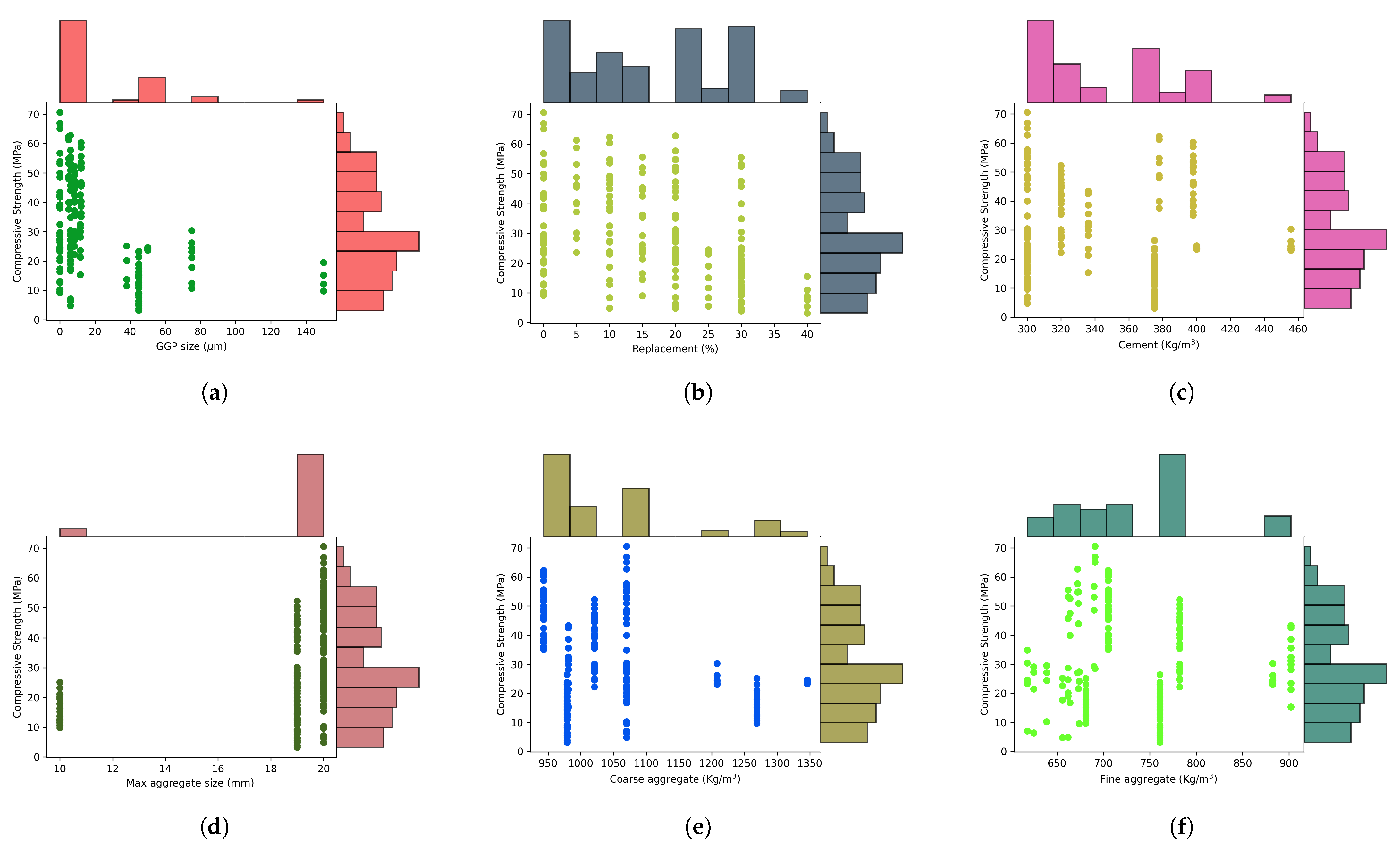
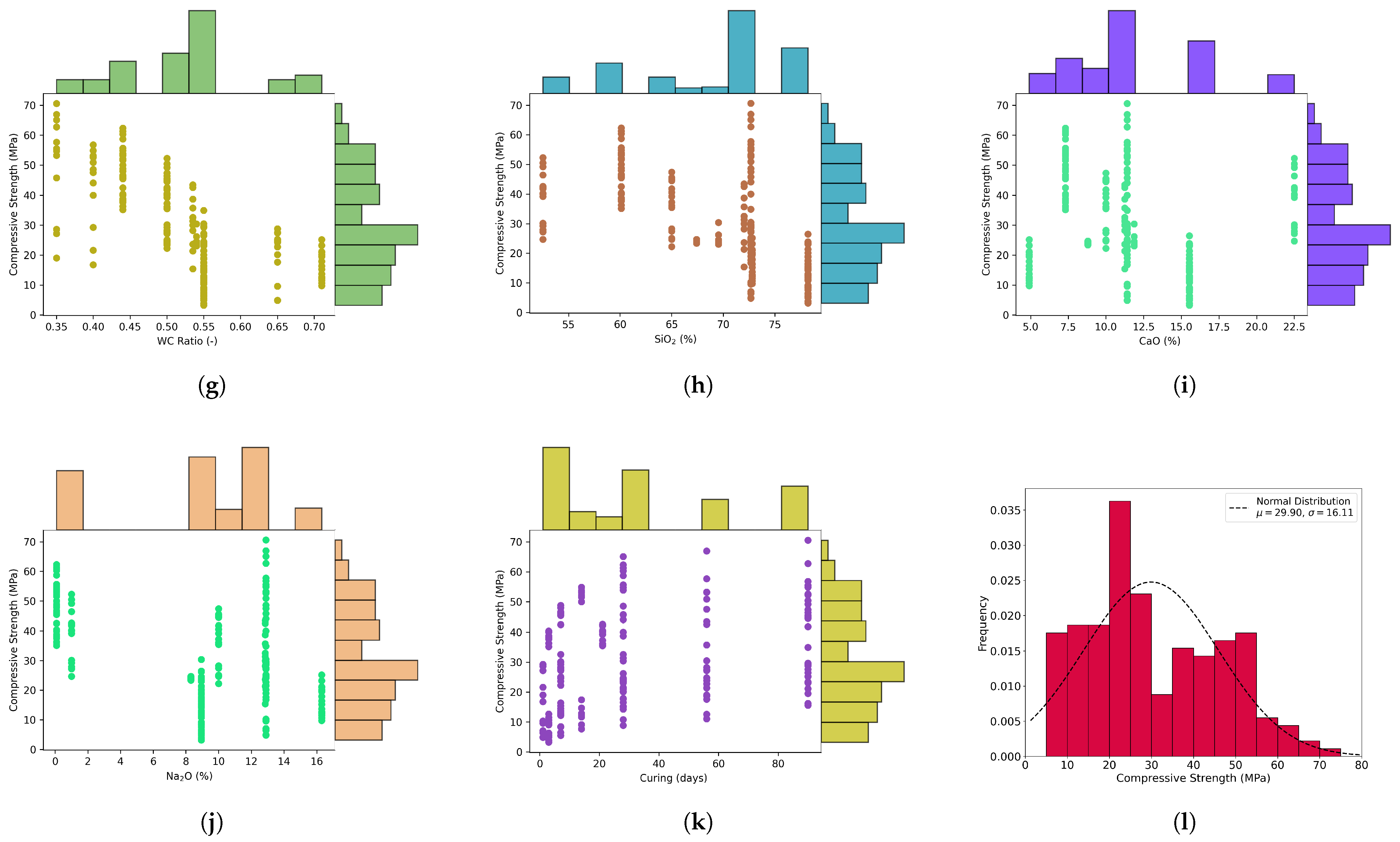
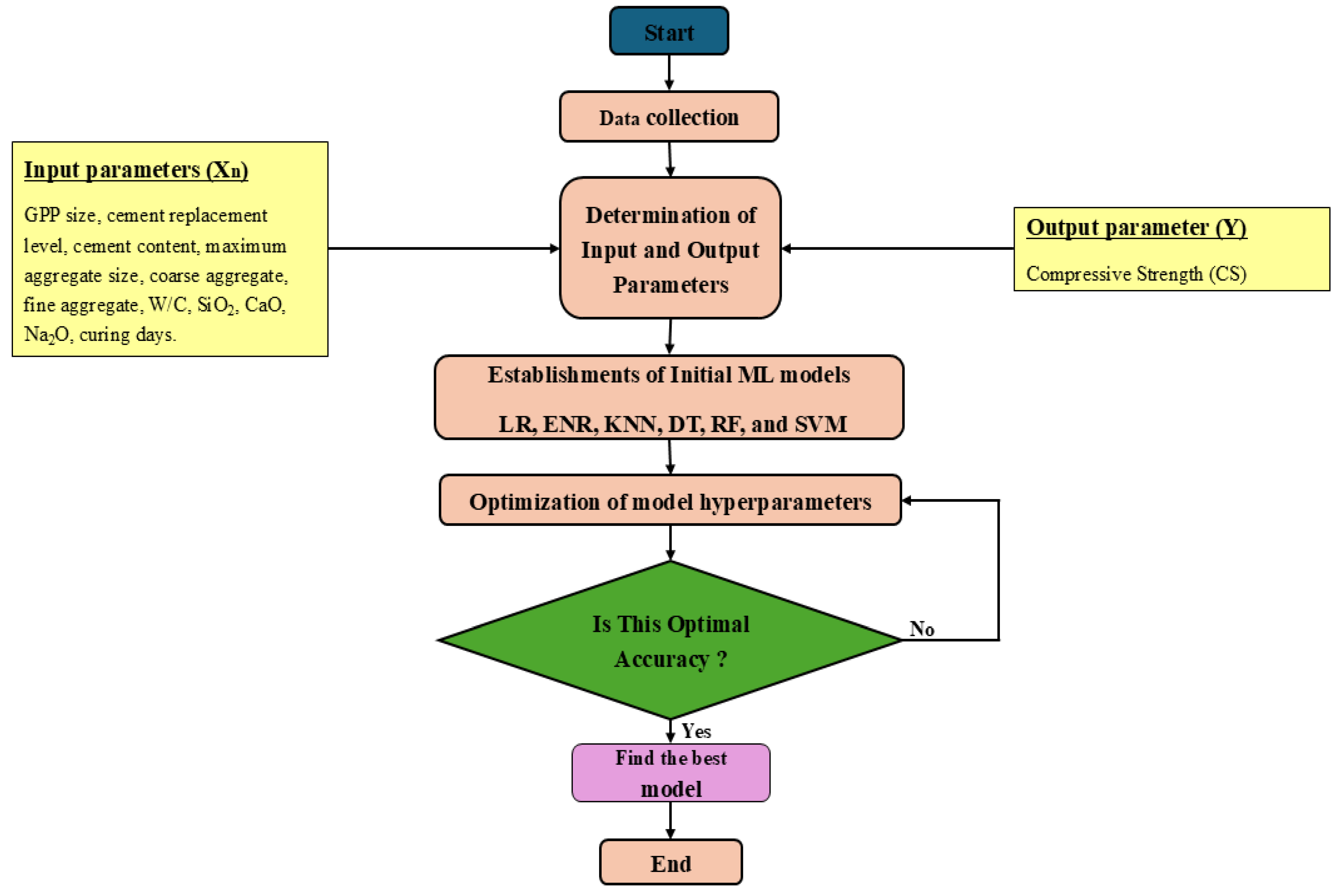
2.1. Data Collection and Preparation

To establish a robust machine learning architecture capable of predicting the CS of concrete incorporating GGP, a broad collection of experimental data was required. Initially, 187 pertinent data points from various available peer-reviewed studies published between 2010 and 2024 [52,53,54,55,56,57,58,59] were collected, each reporting experimental results on the CS of concrete cylinders. The selection of the literature was limited to studies that met the following preliminary criteria: (i) incorporation of GGP derived from post-consumer waste glass in concrete; (ii) utilization of GGP as a partial cement replacement in concrete; (iii) inclusion of standard mix design details and curing procedure; and (iv) reporting of GGP chemical composition. Figure 1 provides comprehensive details on the quantity of data from each study and the percentage contribution to the total dataset. The GGP-incorporated concrete included twelve parameters, i.e., GGP size, GGP replacement level, water-to cement ratio (W/C), cement content, maximum aggregate size, quantity of coarse and fine aggregates, curing time, GGP chemical composition such as SiO₂, calcium oxide (CaO), sodium oxide (Na₂O), and the corresponding CS. The water-reducing admixture, which influences the compressive strength of concrete by modifying the water demand, was excluded in this study due to inconsistent data reporting across the literature.

Once the data were acquired, a basic pre-processing step was performed to prepare them for utmost dependability and consistency. The full dataset comprising 187 concrete mix designs included a total of 2057 data values as input parameters. The subset of this dataset on the GGP chemical composition consisted of 561 individual values across oxide constituents. Among these, 60 values were missing and not reported in the original literature source. Missing values in the dataset were imputed using the mean values of the respective parameters to ensure data integrity and uninterrupted model training. Furthermore, all of the parameters were numerical and appropriate in their original form; no further scaling, encoding, or outlier treatment of datasets was performed. A total of 11 input variables (X = { X₁, X₂, X₃, …, X₁₁}) and 1 output variable (Y) were considered as a final dataset. The unit, minimum/maximum value, mean, standard deviation (SD), and types of the parameters are listed in

Table 2. Compressive strength test parameters.

Parameter	Unit	Minimum	Maximum	Mean	SD	Type
X1: GGP Size	$\mathsf{\mu }$m	5	150	27.23	29.65	Input
X2: Replacement	-	5	40	19.79	11.64	Input
X3: W/C	-	0.35	0.71	0.5	0.09	Input
X4: Cement	kg/m3	300	455.59	343.82	42.74	Input
X5: Max size	mm	10	20	18.75	2.72	Input
X6: Coarse aggregate	kg/m3	943.1	1346	1045.82	103.32	Input
X7: Fine aggregate	kg/m3	618	902	732.50	72.88	Input
X8: SiO2	%	52.5	78.21	69.52	7.70	Input
X9: CaO	%	4.9	22.5	11.87	4.48	Input
X10: Na2O	%	0.08	16.3	8.93	5.16	Input
X11: Curing time	days	1	90	33.22	30.85	Input
Y: Compressive strength	MPa	3.19	70.6	29.90	16.11	Output

.

The marginal plot of the input variables (X_n) and output parameter (Y) using Matplotlib library [60] are depicted in Figure 2. The upper and right portions of the individual subfigure represent the marginal histogram of the respective input variable and CS, while the central scatter plot illustrates the relationship between each input parameter with target variable (CS). The GGP size ranges from 5 to 150 $\mathsf{\mu }$m, with the majority concentrated between 5 and 20 $\mathsf{\mu }$m. The cement replacement level is uniformly distributed across 5% to 40%, and cement content varies from 300 to 460 kg/m³. Furthermore, the maximum aggregate size ranges from 10 to 20 mm with the majority of values clustered around 19–20 mm. The coarse aggregate and fine aggregate falls in broader ranges of 940–1350 kg/m³ and 615–905 kg/m³, respectively. Additionally, the W/C ratio is uniformly distributed from 0.35 to 0.71. Among the oxides, SiO₂ ranges from 50% to 80%, with the majority lying between 70% and 75%. The CaO and Na₂O range in between 4.9–22.5% and 0.08–16.3%, respectively. The curing days range from 1 to 90 days, with most data concentrated between 1 and 28 days. The CS values range from 3.19 to 70.6 MPa, with a mean value of 29.9 MPa and a standard deviation of 16.11 MPa.

A Pearson correlation matrix for input parameters and the output parameter using seaborn library [61] was constructed by examining the linear relationship between parameters as illustrated in Figure 3. The color gradient represents correlation coefficient values ranging from −1 to +1. Darker shades represents stronger correlation (either positive or negative) between the input features. The +1 indicates a perfect positive correlation, −1 represents a perfect negative correlation, and 0 signifies no correlation between parameters. The matrix helps identify highly correlated input variables and mitigate the influence of multicollinearity (correlation coefficient |r| > 0.8) [62]. Among the parameters, the most significant positive and negative correlation were found between Na₂O and SiO₂ (r = 0.73), the W/C ratio, and the compressive strength (r = −0.68). This inverse relationship is well established in concrete technology. A higher W/C ratio increases the porosity in concrete matrix, which reduces the density and compressive strength of the hardened concrete [63].

2.2. Machine Learning Models

Six different machine learning models, LR, ENR, KNN, DT, RF, and SVR, were considered in this study. For machine learning modeling, eleven concrete parameters from different studies were taken as inputs, and the CS as an output. The open source Scikit-Learn library [64] in the Python programming language (version 3.12.4) [65] was utilized. A flowchart illustrating the workflow of finding the best ML algorithm is depicted in Figure 4. The training and testing datasets were divided at a ratio of 80:20. The grid search technique was utilized to tune the hyperparameters and improve the accuracy of models. Additionally, 5 k-fold cross validation was implemented to ensure the robustness of the model on different subsets of data. The theory of individual ML models used and hyperparameter tuning associated with the respective model are briefly described in the upcoming section.

2.2.1. Linear Regression (LR)

Regression models are widely used to quantify the patterns of interactions between predictor and dependent variables and to assess their degree of correlation [66]. One dependent variable and one independent predicting variable make up a simple LR model, illustrating a linear connection between two variables. On the other hand, the multiple LR model involves a single dependent variable predicted by a number of independent variables. Equation (1) illustrates the relationship between dependent and independent variables:

$$Y={\beta }_0+{\beta }_1{X}_1+{\beta }_2{X}_2+\cdots +{\beta }_n{X}_n+ϵ\Rightarrow Y=MX+C$$

(1)

where Y denotes the dependent variable, $X_1,X_2,\dots ,X_n$ represent the independent variables, ${\beta }_0$ is the intercept term [67], ${\beta }_1,{\beta }_2,\dots ,{\beta }_n$ are the regression coefficients, and $ϵ$ accounts for the error in the model.

2.2.2. ElasticNet Regression (ENR)

Regularization techniques are widely utilized to address the overfitting issues and handle high-dimensional feature spaces to improve model generalization. ElasticNet regression (ENR), an LR model, synergistically combines L1 (Lasso) and L2 (Ridge) regularization techniques. In the case of L2 regularization, the penalty term is defined by the L2-norm of $\beta$, and in L1 regularization, the penalty is defined by the L1-norm [68]. Furthermore, these penalties are referred to as ridge regression (least absolute shrinkage) and lasso regression (selection operator). The Elastic Net cost function is given by

$$J\left(\theta \right)={\displaystyle \frac{1}{2m}}\sum _{i=1}^m{(y_i-h_{\theta }\left(x_i\right))}^2+\alpha \left[\rho \sum _{j=1}^n\left|{\theta }_j\right|+(1-\rho )\sum _{j=1}^n{\theta }_j^2\right]$$

(2)

or equivalently, using ${\lambda }_1$ and ${\lambda }_2$:

$$J\left(\theta \right)={\displaystyle \frac{1}{2m}}\sum _{i=1}^m{(y_i-h_{\theta }\left(x_i\right))}^2+{\lambda }_1\sum _{j=1}^n\left|{\theta }_j\right|+{\lambda }_2\sum _{j=1}^n{\theta }_j^2$$

(3)

where

$${\lambda }_1=\alpha \rho ,{\lambda }_2=\alpha (1-\rho )$$

• $\alpha$: overall regularization strength (same as ‘alpha’ in ‘ElasticNet (alpha=…)’).
• $\rho$: mixing parameter, controlling the balance between L1 and L2 regularization.
• ${\lambda }_1$: coefficient for L1 (lasso) regularization, derived from $\alpha \rho$.
• ${\lambda }_2$: coefficient for L2 (ridge) regularization, derived from $\alpha (1-\rho )$.

Hyperparameter alpha plays a crucial role in tuning the overall strength of the regularization. Smaller values of alpha reduce the impact of the penalty terms. Similarly, ratio L1, which is 0.987 in this case, helps determine the best balance between L1 and L2 regularization. The closer it is to 1, the more it will tend towards lasso, which is great for sparsity induction in feature selection.

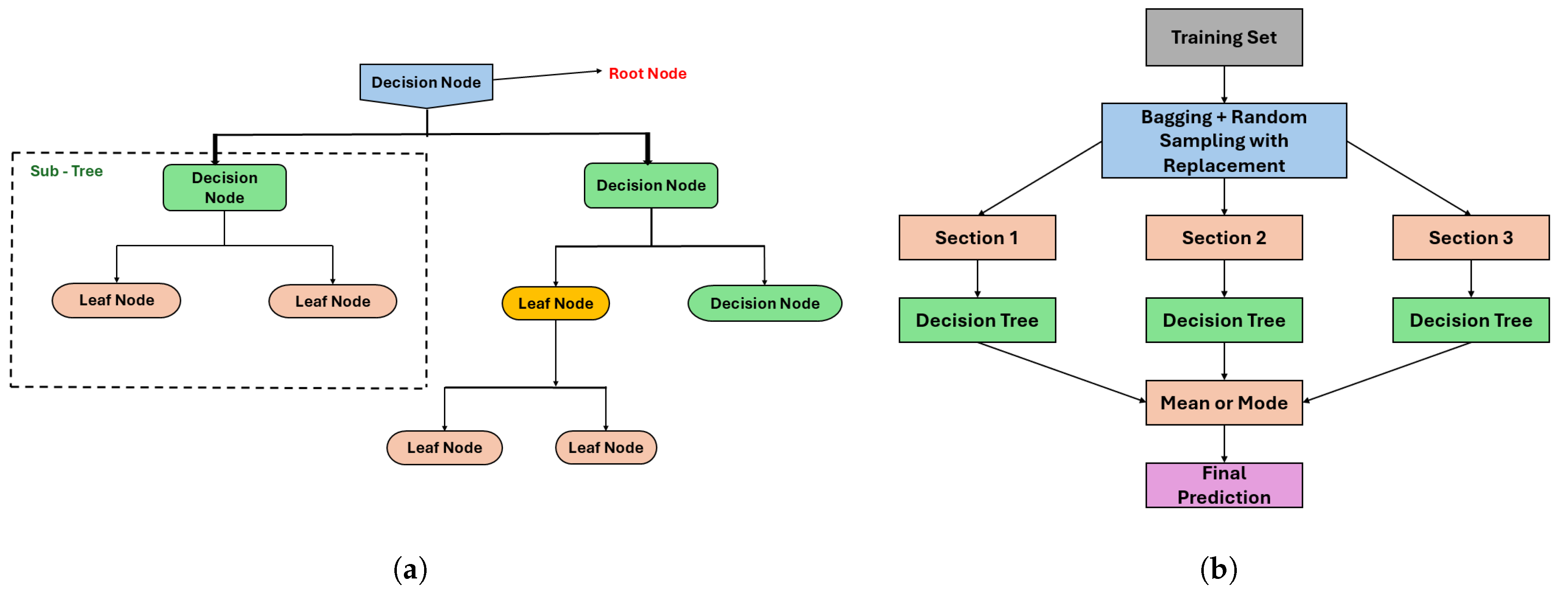
2.2.3. Decision Tree Regressor (DT)

DT is one of the effective and comprehensible machine learning methods used to forecast continuous outcomes as depicted in Figure 5a. The DT regressor divides the feature space into multiple sub-regions and assigns a constant value to each region for modeling, in contrast to classic regression techniques that fit a single global model to represent the data [69]. The multiple sub-regions are formed through recursive partitioning based on the feature value. Furthermore, optimal splits are determined by minimizing error metrics such as the mean square error (MSE), root mean square error (RMSE), etc. Each internal node represents a decision based on a feature, each branch denotes the decision’s outcome, and each leaf node corresponds to a predicted value, collectively structured like a tree.

A key benefit of decision trees over other modeling approaches is their ability to generate models that can be expressed as interpretable rules or logical statements. The interpretability of trees that create axis-parallel decision boundaries offers a significant advantage [70]. Additionally, classification using decision trees does not require complex computation, and the method is applicable to both continuous and categorical variables. Moreover, decision tree models offer transparent insights into the relative importance of key factors in prediction or classification tasks.

In this study, the hyperparameter maximum depth limits the number of splits to avoid overfitting, as deeper trees tend to capture intricate patterns; however, it may overfit on small datasets. The criterion (for example, gini impurity for classification or squared error for regression) determines the splitting points for impurity reduction and optimization. Additionally, the minimum sample split parameter controls the minimum number of samples required to split a node, preventing unnecessary splits. Furthermore, the minimum sample leaf parameter ensures that each leaf node has at least a minimum number of samples, aiding in generalization by mitigating highly specific decision rules.

2.2.4. Random Forest Regressor (RF)

RF is a predictor consisting of an assortment of ‘M’ randomized regression trees, where a random subset of training data are used to construct each tree. The term “random forests” can be interpreted in different ways. Some scholars describe it as a generic expression for aggregating random decision trees regardless of how trees are obtained, while others refer to the original algorithm [71]. RF is an ensemble learning technique that combines multiple decision trees to increase accuracy and reduce overfitting as illustrated in Figure 5b. Similarly, trees are generated independently, allowing the process to be parallelized for better computation. Unlike a single decision tree that is prone to the overfitting problem, the RF model leverages bagging (Bootstrap Aggregation) and random feature selection to reduce variance while maintaining interpretability. Mathematically, RF follows the bagging approach, where each individual tree is trained on a bootstrapped dataset drawn from the original dataset [72].

$$D={\left\{(X_i,Y_i)\right\}}_{i=1}^N$$

(4)

where $X_i$ represents feature vectors, and $Y_i$ represents the target values. Each tree $T_b$ is trained on a subset $D_b$ of the original data, and each subset $D_b$ is drawn randomly from D with replacement.

For regression, the final prediction $\widehat{Y}$ is obtained by averaging the predictions from all B trees:

$$\widehat{Y}={\displaystyle \frac{1}{B}}\sum _{b=1}^B{T}_b\left(X\right)$$

(5)

The hyperparameter “number of trees” is controlled with the estimator parameter. The increasing number of trees enhances the predictive performance; however, it results in higher computational expense. Minimum samples split and minimum samples per leaf operate as pruning parameters [73] for decision trees, controlling the growth of trees and pruning. Furthermore, max feature controls the number of features considered for splitting in each step to reduce overfitting through the application of diversity across trees. Bootstrap sampling controls training each tree on a random subsample of data that reduces the variance and promotes generalization in the model.

Figure 5. Graphical representation of (a) DT [74] and (b) RF [75].

Figure 5. Graphical representation of (a) DT [74] and (b) RF [75].

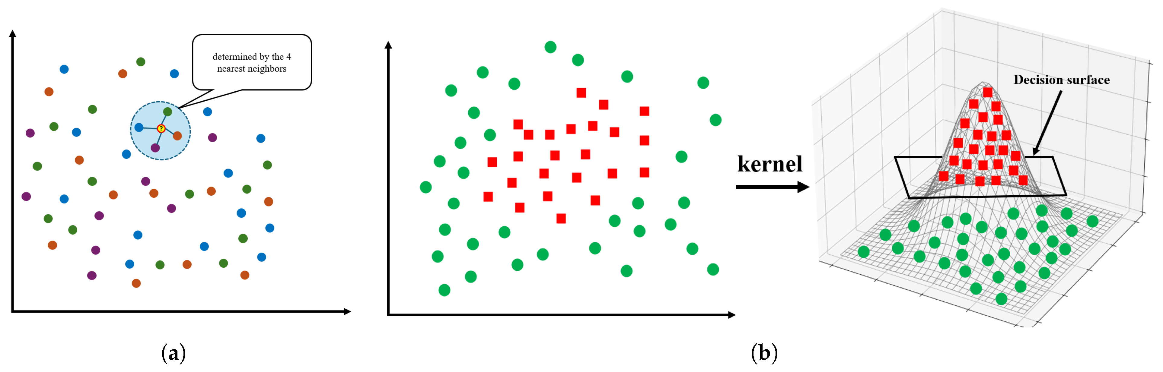
2.2.5. K-Nearest Neighbor Regressor (KNN)

K-Nearest Neighbor is a basic machine learning algorithm that can be implemented for classification and regression tasks [76]. It is a supervised learning method that operates on the idea that data points with similar features are located in near proximity of each other within a feature space as depicted in Figure 6a. In KNN Regression, the prediction for a new data point is obtained by averaging the target values of its closest neighbors, which are identified using a distance metric such as the Euclidean or Manhattan distance.

The KNN algorithm predicts outcomes through a simple process, as illustrated in Figure 6a. Initially, the number of neighbors (k) is considered [77], followed by a distance metric, typically Euclidean distance, to identify the ‘k’ closest points in the training dataset. Once the nearest neighbors are identified, their output values are averaged (or weighted) to generate the prediction. The expected value $\widehat{y}$ can be expressed mathematically as

$$\widehat{y}={\displaystyle \frac{1}{k}}\sum _{i=1}^k{y}_i$$

(6)

where $y_i$ represents the actual output values of the k-Nearest Neighbors.

In this study, hyperparameter neighbor k considers the k nearest points for the prediction to balance between the bias and variance. When k is small, the model becomes sensitive to noise, whereas larger k results in a smoother decision boundary. Similarly, hyperparameter ‘p’ indicates the distance method determined to calculate the distance between points [78]. Furthermore, the weights parameter determines the contribution of the selected neighbor to calculate the output. For instance, in weighted schemes, closer neighbors have more influence on the decision, whereas in uniform schemes, every neighbor has equal weight.

2.2.6. Support Vector Regressor (SVR)

SVR is a machine learning algorithm that is derived based on the support vector machine (SVM) principles for regression analysis. A standard classification SVM locates a hyperplane to separate, different classes with maximum margins [79]. However, SVR computes a specific function that stays close to all data points, as illustrated in Figure 6b. The algorithm maintains a small margin of error epsilon ($\epsilon$), making the SVR method effective for precise numerical predictions instead of category assignments. The equation provided to minimize the cost function in SVR is

$$min{\displaystyle \frac{1}{2}}{\parallel w\parallel }^2+C\sum _i\left({\xi }_i+{\xi }_i^{*}\right)$$

(7)

$$\mathrm{Subject}\mathrm{to}:y_i-w^T{x}_i-b\le ϵ+{\xi }_i$$

(8)

$$w^T{x}_i+b-y_i\le ϵ+{\xi }_i^{*}$$

(9)

$${\xi }_i,{\xi }_i^{*}\ge 0$$

(10)

where

-

${\parallel w\parallel }^2$ controls the model complexity.

-

C is a hyperparameter that determines the trade-off between margin size and prediction accuracy.

-

${\xi }_i=max\left(0,f\left(x_i\right)-y_i-ϵ\right)$.

-

${\xi }_i^{*}=max\left(0,y_i-f\left(x_i\right)-ϵ\right)$.

-

${\xi }_i,{\xi }_i^{*}$ are the Slack variables that penalize the error if the prediction is outside the $\le ϵ$ margin.

In this study, parameter ‘C’ controls the trade-off between maximizing the margin and minimizing error. Higher values of C result in a high penalty for misclassifications, making tighter decision boundaries [80]. Epsilon ($ϵ$) demonstrates relevance in regression-based SVR to define the error tolerance in regression [81]. Similarly, a kernel function (linear, polynomial, radial basis function (RBF), etc.) transforms the input into a higher-dimensional space, making it easier to identify patterns in the data. The gamma parameter controls the influence of individual training points on the decision boundary, such that smaller values result in wider decision boundaries and higher values provide priority to local patterns [82]. Thus, hyperparameter tuning is essential for better predictive accuracy as well as model adaptability.

Figure 6. Graphical representation of (a) KNN [83] and (b) SVR [84].

Figure 6. Graphical representation of (a) KNN [83] and (b) SVR [84].

2.3. Error Computation

Many studies employ the mean square error (MSE) and its rooted variant root mean square error (RMSE), or the mean absolute error (MAE) and its percentage variant (MAPE), as error-based metrics to evaluate the model performance. Although widely utilized due to their simplicity and interpretability, these metrics share a common drawback: unbounded values ranging between zero and positive infinity. Furthermore, a single value provides limited insight into the performance of the regression models with respect to the statistical distribution of the ground truth elements [85]. This study utilizes two primary metrics, RMSE and R² error (coefficient of determination), for the evaluation of the model performance. RMSE quantifies the square root of the squared average differences between observed values with predicted values, resulting in a comprehensive measure of prediction accuracy. A lower RMSE reflects lower deviations between actual and predicted values and indicates better model performance. Mathematically, it is given by

$$RMSE=\sqrt{{\displaystyle \frac{1}{N}}\sum _{i=1}^N{(Y_i-{\widehat{Y}}_i)}^2}$$

(11)

On the other hand, the coefficient of determination (R² error) quantifies the extent to which the independent variables explain the variance in the dependent variable. It is computed as

$$R^2=1-{\displaystyle \frac{\sum {(Y_i-{\widehat{Y}}_i)}^2}{\sum {(Y_i-\overline{Y})}^2}}$$

(12)

A value of R² closer to 1 indicates an excellent model fit, whereas a lower R² reflects weak predictive capabilities. Unlike RMSE, which measures predictive error in absolute terms, R² offers a relative assessment by comparing model performance against a baseline—the mean of the target variable. RMSE and R² serve different purposes in regression analysis: while RMSE measures the accuracy of predictions in absolute terms, R² explains how variance in the target variable is captured by the model. Collectively, these metrics enable the capture of both the magnitude of prediction errors and the overall goodness of fit.

2.4. Hyperparameter Tuning

Hyperparameter tuning has a direct influence on models’ predictive capabilities and is an important step in optimizing model-governing parameters. However, the determination of the best hyperparameters can be computationally intensive, particularly when the determination of objective functions is costly or when the model requires the tuning of a large number of parameters [86]. Several effective techniques are available for tuning hyperparameters in ML methods, such as grid search (GS), random search (RS), Bayesian optimization (BO), etc.

In this study, the GS optimization method was utilized for hyperparameter tuning due to the lower number of parameters involved with the employed ML models. It is often described as a brute-force or exhaustive search technique [87]. While GS is known for its high accuracy, the computational time required for it is excessive. Grid search (GS) exhaustively searches a manually specified subset of the hyperparameter space of the target algorithm. Unlike RS, which may miss critical combinations due to random sampling from the hyperparameter space, GS evaluates all possible combinations within the predefined grid, offering a more reliable optimization approach. Furthermore, for a smaller dataset and fewer associated hyperparameters, BO, with its complexity in setting up surrogate models and acquisition functions, makes it less efficient in this study in comparison to GS.

3. Results and Discussion

The CS of GGP-incorporated concrete was analyzed using six individual supervised ML algorithms. The measured CS versus the predicted CS is plotted for each ML algorithm. Figure 7 illustrates the results of the training and testing datasets for LR, ENR, KNN, DT, RF, and SVR. The RMSEs are 6.95 MPa, 8.20 MPa, 6.56 MPa, 3.88 MPa, 5.70 MPa, and 8.01 MPa for LR, ENR, KNN, DT, RF, and SVR, respectively, for the testing dataset. Similarly, for the test dataset, the R² values for LR, ENR, KNN, DT, RF, and SVR are 0.80, 0.73, 0.82, 0.94, 0.86, 0.74, respectively. The DT model predicted the best among the six ML algorithms with an R² of 1.0 for the training dataset and R² of 0.94 for the testing dataset. However, this perfect R² value in the training dataset is due to overfitting, a problem commonly encountered by the DT model when no constraints are provided. When hyperparameters are not tuned, the DT model is highly flexible and tends to split the dataset until all data are perfectly fitted. This leads to the formation of deeper trees that extend until each leaf contains only one data point. Thus, the DT model tends to memorize the dataset along with noise, and ultimately yields reduced performance on the unseen testing dataset. For RF, before hyperparameter tuning, the algorithm yielded an R² of 0.88 for training and 0.82 for the testing dataset, with an RMSE of 5.56 MPa for training and 6.55 MPa for the testing dataset. Although RF demonstrated relatively better performance compared to the other ML models, the slight variation in error metrics between the testing and training dataset suggests potential overfitting. Furthermore, the R² values for LR and ENR before hyperparameter tuning for the testing dataset are below 0.8, which is generally not considered a good fit. Furthermore, KNN and SVR demonstrate moderate generalization capabilities before tuning. RMSE values of 6.69 MPa for training and 6.56 MPa for testing by KNN indicate suboptimal performance. Additionally, a high discrepancy between training (RMSE = 5.85 MPa) and testing (RMSE = 8.01 MPa) suggests underfitting for the SVR model. Similarly, LR and ENR demonstrate a stable, yet moderate performance with similar RMSE values. LR achieved RMSE values of 5.56 MPa and 6.95 MPa for training and testing datasets, respectively, while ENR obtained RMSE values of 8.27 MPa and 8.20 MPa. This suggests lower overfitting problems; however, the prediction accuracy is lower than that of the other models.

The predictive capability of five models, ENR, KNN, DT, RF, and SVR, after respective model hyperparameter tuning is depicted in Figure 8. All machine learning models demonstrate R² values greater than 0.8 for the test dataset, which is generally considered a good fit. ENR shows a significant increase in its R² from 0.73 to 0.81 with the reduction in RMSE from 8.20 to 6.85 MPa for the test dataset. Similarly, the KNN algorithm also improves performance with an increase in the R² value from 0.82 to 0.87. Furthermore, the DT model, which initially exhibited a perfect fit on the training data (R² = 1 and RMSE = 0.0 MPa), demonstrates better generalization with balanced training and testing R² values of 0.98 and 0.91, respectively. This is achieved through pre-pruning in the DT algorithm, where hyperparameters such as maximum tree depth, minimum samples split, and minimum samples per leaf are optimized to control the tree growth to mitigate the overfitting problem. The RF model, after hyperparameter tuning, shows improvement in both testing and training performance. The RMSE drops from 6.55 MPa to 4.56 MPa and R² increases from 0.82 to 0.91 for the test dataset, reflecting better predictive accuracy after hyperparameter tuning. SVR benefits greatly from hyperparameter tuning and demonstrates the highest predictive capabilities among the models with an R² value of 0.95 and RMSE of 3.40 MPa for the test dataset. For a small dataset with high dimensionality, SVR outperforms other algorithms such as KNN and DT due to its robustness against the curse of dimensionality. Similarly, for a non-linear dataset, the kernel trick in SVR enables the algorithm to effectively model the complex patterns in higher-dimensional spaces. By tuning hyperparameters such as regularization parameter C and loss parameter $ϵ$, SVR can fine-tune the balance between fit and generalization, making it less susceptible to overfitting or underfitting problems. The RMSE of 3.40 MPa from the SVR algorithm in this study is slightly higher than the RMSE of 2.447 MPa reported by Seghier et al. [50]. This difference could be attributed to the use of hybrid metaheuristic optimization (MPA) utilization for hyperparameter tuning, which offers enhanced predictive capabilities compared to conventional grid search tuning employed in this study. Furthermore, the present study considers a broader range of input parameters, including the chemical composition of GGP, which further increases the model complexity.

The performance of the six ML models employed in this study before and after hyperparameter tuning is shown in

Table 3. Model performance before and after hyperparameter tuning.

Model	Before Hyperparameter Tuning				After Hyperparameter Tuning
	Training Data		Testing Data		Training Data		Testing Data
	RMSE	R2	RMSE	R2	RMSE	R2	RMSE	R2
Linear Regression	5.56	0.88	6.95	0.80	–	–	–	–
ElasticNet Regression	8.27	0.73	8.20	0.73	5.57	0.88	6.85	0.81
K-Nearest Neighbor	6.69	0.82	6.56	0.82	3.83	0.94	5.62	0.87
Decision Tree	0.00	1.00	3.88	0.94	2.08	0.98	4.65	0.91
Random Forest	5.56	0.88	6.55	0.82	2.23	0.98	4.56	0.91
Support Vector Regressor	5.85	0.86	8.01	0.74	2.00	0.98	3.40	0.95

. The higher RMSE in LR and ENR compared to the other models can be attributed to their limitation in capturing the non-linearity in the current dataset. Similarly, due to the sensitivity to irrelevant features and the curse of dimensionality, the KNN model demonstrates higher RMSE values than DT, RF, and SVR. For the DT model, its the maximum depth limitation and pruning effect give moderate RMSE values compared to the other models. The RF, which is an ensemble of multiple DT models, helps in better generalization by reducing variance and lowering the RMSE compared to the DT model. Finally, SVR demonstrates the lowest value of RMSE due to its robustness in modeling a more complex non-linear dataset using a kernel-based approach. Furthermore, finalized hyperparameters associated with each model are summarized in

Table 4. Finalized hyperparameters.

ENR	KNN	DT	RF	SVR
alpha = 0.01	Neighbors = 3	Max depth = 7	No. of estimators = 79	C = 100
L1 ratio = 0.987	p = 2	criterion = squared error	Minimum samples splits = 2	Epsilon = 0.1
	Weights = uniform	Min samples split = 3	Minimum samples leaf = 1	Kernel = rbf
		Min samples leaf = 2	bootstrap = False	Gamma = 0.1

. Overall, hyperparameter tuning enhances the model performance of all models, reduces the underfitting and overfitting problems, and improves the model predictability for testing and training datasets.

The SHapley Additive exPlanations (SHAP) [88] plot illustrated in Figure 9 demonstrates the importance of individual input variables in predicting the CS of concrete incorporating GGP using the SVR algorithm. SVR was selected for SHAP analysis due to its superior predictive accuracy among the evaluated models. An individual dot represents a SHAP value for a particular feature and instance [89]. The x-axis, y-axis, and color represent a feature’s impact on the predicted output, the ranking of the features’ importance from top to bottom, and actual feature values (blue for low, red for high), respectively. The SHAP plot result shows that the curing time (Days) has the most positive influence, while the W/C ratio has the most negatively impact on strength predictions. This aligns with understanding conventional concrete behavior. Furthermore, the SiO₂, Na₂O, replacement level, and GGP size demonstrate an inverse relationship with the predicted compressive strength. Nonetheless, variables such as CaO, FA, cement content, CA, and maximum aggregate size have a relatively minor influence on the model.

4. Conclusions

Accurately estimating the CS of concrete is essential for optimizing mix designs, reducing curing durations, and minimizing overall project costs. In this study, different ML algorithms: linear regression, ElasticNet regression, a K-Nearest Neighbor Regressor, a decision tree regressor, a random forest regressor, and a support vector regressor, were employed, leveraging 11 influencing input parameters from 187 reliable mixes to predict the CS of concrete. The results indicate favorable evidence of using artificial intelligence approaches to predict the CS of concrete incorporated with GGP as a partial cement replacement. The following conclusions are drawn after careful evaluation of each model’s performance:

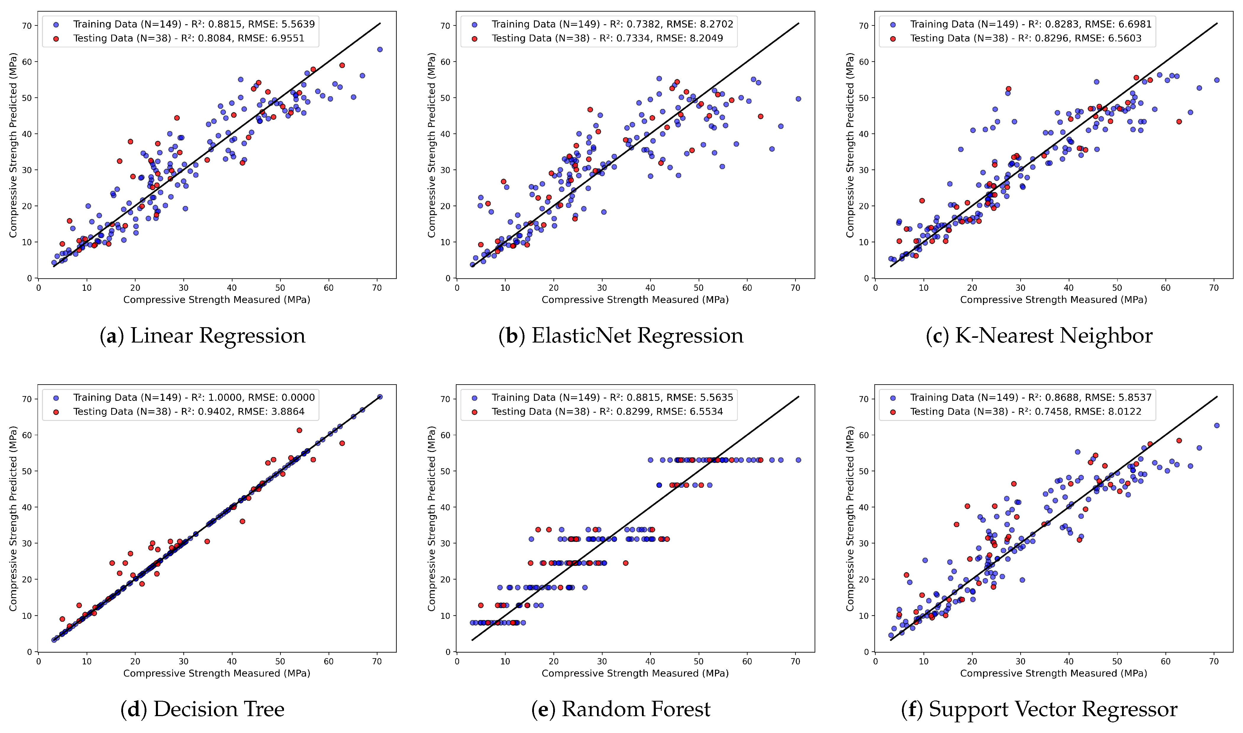
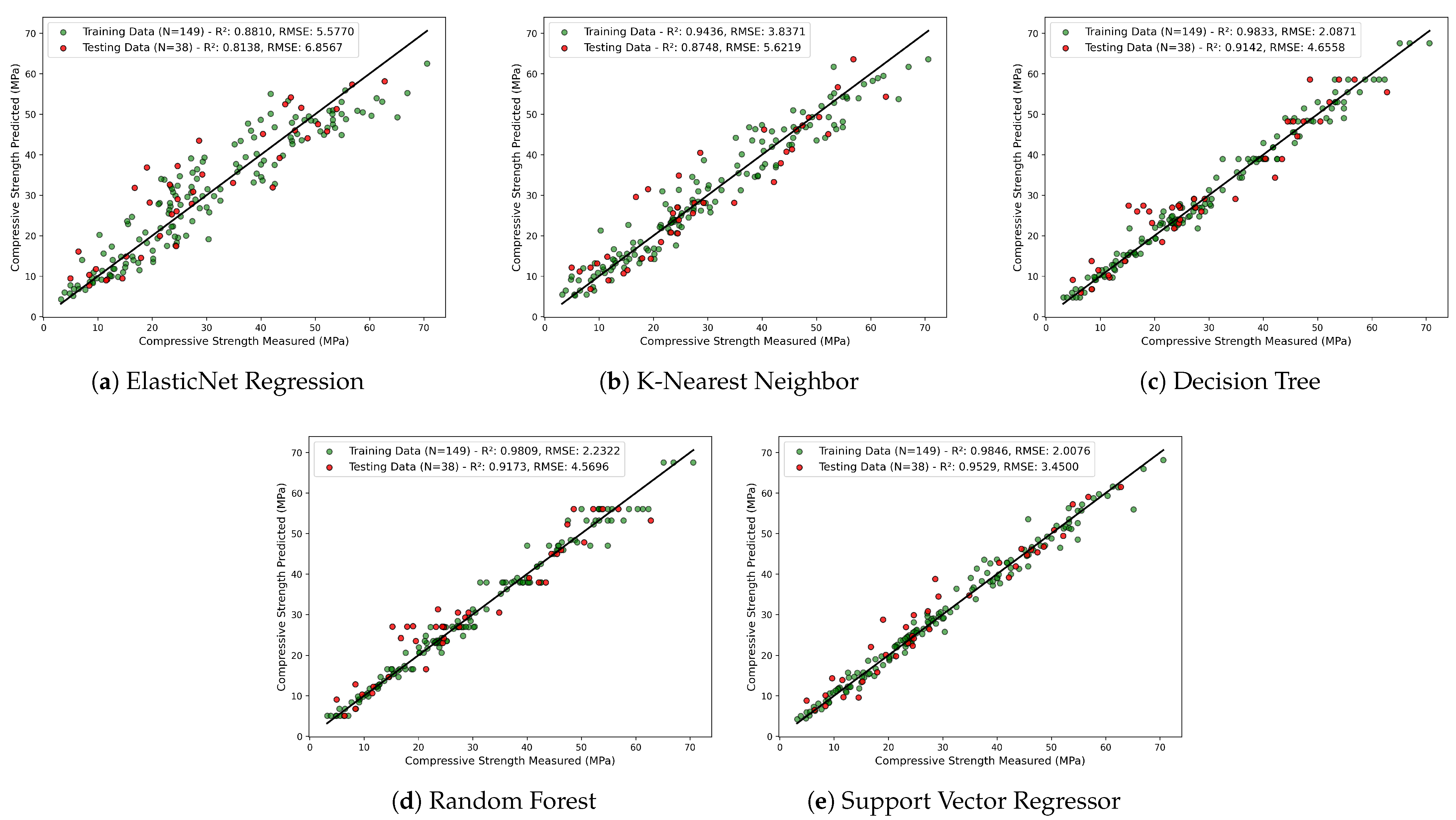
• Linear regression and ElasticNet regression exhibit stable yet moderate performance with similar R² and RMSE values before hyperparameter tuning. However, ElasticNet regression shows a significant increase in the R² value from 0.73 to 0.81 with a drop in RMSE value from 8.20 to 6.85 MPa for the test dataset after hyperparameter tuning.
• The K-Nearest Neighbor regressor model shows good prediction with the same R² value of 0.82 for training and testing before hyperparameter tuning. Furthermore, with hyperparameter tuning, the R² value increased to 0.87 and RMSE decreased to 5.62 MPa for the test dataset.
• The decision tree regressor demonstrates the highest accuracy (R² = 1.0 for training, R² = 0.94 for testing) before hyperparameter tuning due to the creation of deep trees. A reduction in overfitting and better generalization with training and testing datasets was achieved through hyperparameter tuning.
• The random forest regressor model exhibits moderate performance with an R² of 0.82 and RMSE of 6.55 MPa for the test dataset. However, after hyperparameter tuning, the RMSE decreased to 4.56 MPa from 6.55 MPa and R² improved to 0.91 from 0.82 for the test dataset. In conclusion, the RF model benefits from hyperparameter tuning, leading to improved generalization.
• Support vector regressor demonstrates lower accuracy with an R² of 0.74 and RMSE of 8.01 MPa for the test dataset before hyperparameter tuning. However, a significant increase in R² to 0.95 and a reduction in RMSE to 3.40 MPa show the superior predictive capability of SVR after hyperparameter tuning.
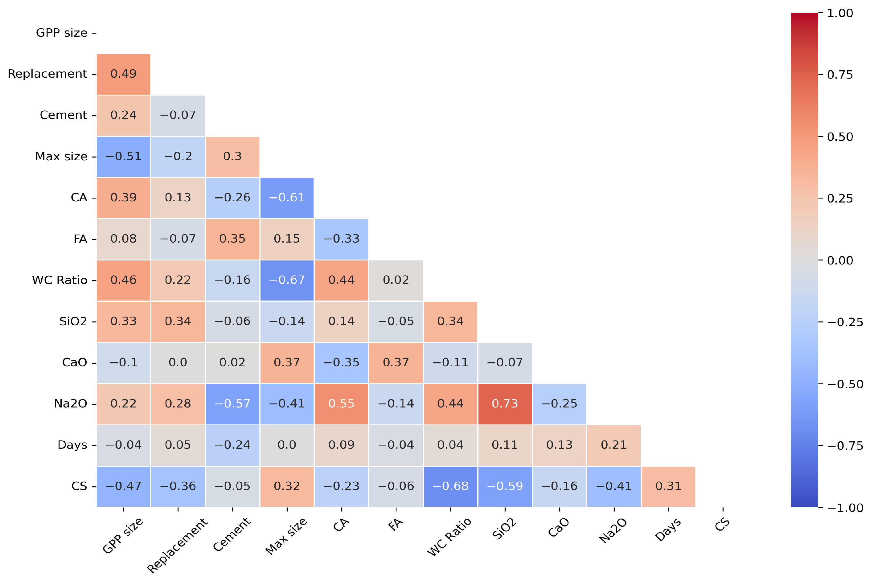
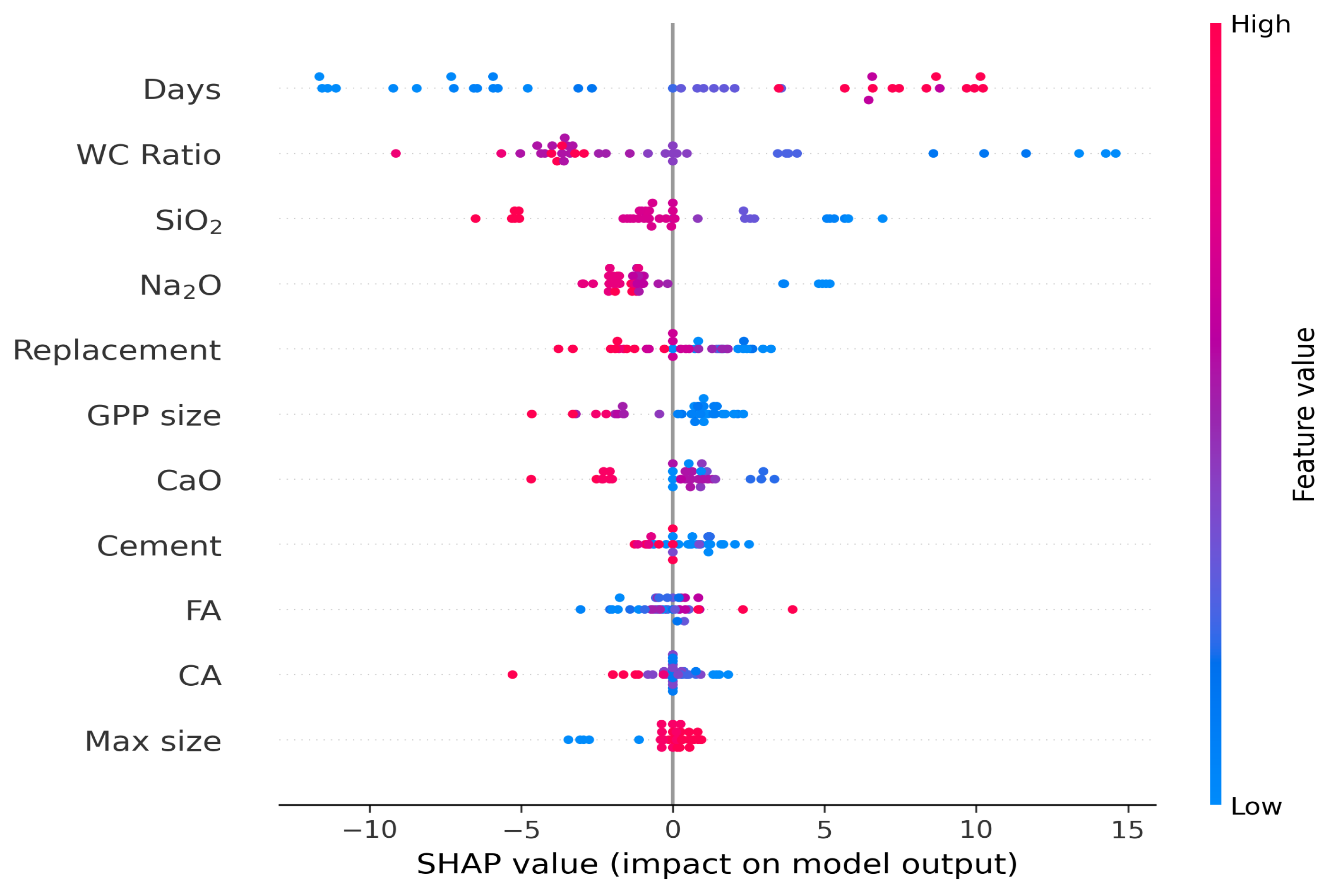
• SHAP analysis shows that curing time has the most significant positive influence, while the W/C ratio has the most significant negative influence on the prediction of CS for the SVR algorithm.

In conclusion, the ML models demonstrate reliable predictive accuracy on estimating the CS of GGP-incorporated concrete. The practical implications of these findings can be a significant help in promoting sustainability within the construction industry. These models enable the optimization of GGP content in concrete mix designs, thereby reducing cement demand and associated CO₂ emissions. Furthermore, the use of GGP as an SCM in concrete diverts glass from landfill sites, promoting a circular economy. With the data considered, SVR outperforms other ML algorithms in the prediction of the CS of concrete incorporating GGP. SVR, with its high accuracy, has the potential to serve as a predictive tool for optimizing mix designs, reducing the overall cost of future projects, and supporting sustainable construction practices.

References

1. Feng, D.C.; Liu, Z.T.; Wang, X.D.; Chen, Y.; Chang, J.Q.; Wei, D.F.; Jiang, Z.M. Machine learning-based compressive strength prediction for concrete: An adaptive boosting approach. Constr. Build. Mater. 2020, 230, 117000. [Google Scholar] [CrossRef]
2. Yehia, S.A.; Shahin, R.I.; Fayed, S. Compressive behavior of eco-friendly concrete containing glass waste and recycled concrete aggregate using experimental investigation and machine learning techniques. Constr. Build. Mater. 2024, 436, 137002. [Google Scholar] [CrossRef]
3. Chopra, P.; Sharma, R.K.; Kumar, M.; Chopra, T. Comparison of machine learning techniques for the prediction of compressive strength of concrete. Adv. Civ. Eng. 2018, 2018, 5481705. [Google Scholar] [CrossRef]
4. Elmikass, A.G.; Makhlouf, M.H.; Mostafa, T.S.; Hamdy, G.A. Experimental Study of the Effect of Partial Replacement of Cement with Glass Powder on Concrete Properties. Key Eng. Mater. 2022, 921, 231–238. [Google Scholar] [CrossRef]
5. Abdelli, H.E.; Mokrani, L.; Kennouche, S.; de Aguiar, J.B. Utilization of waste glass in the improvement of concrete performance: A mini review. Waste Manag. Res. 2020, 38, 1204–1213. [Google Scholar] [CrossRef]
6. Muhedin, D.A.; Ibrahim, R.K. Effect of waste glass powder as partial replacement of cement & sand in concrete. Case Stud. Constr. Mater. 2023, 19, e02512. [Google Scholar]
7. Paul, S.C.; Šavija, B.; Babafemi, A.J. A comprehensive review on mechanical and durability properties of cement-based materials containing waste recycled glass. J. Clean. Prod. 2018, 198, 891–906. [Google Scholar] [CrossRef]
8. Khatib, J.; Hibbert, J. Selected engineering properties of concrete incorporating slag and metakaolin. Constr. Build. Mater. 2005, 19, 460–472. [Google Scholar] [CrossRef]
9. Siddique, R. Utilization of silica fume in concrete: Review of hardened properties. Resour. Conserv. Recycl. 2011, 55, 923–932. [Google Scholar] [CrossRef]
10. Safiuddin, M.; West, J.; Soudki, K. Hardened properties of self-consolidating high performance concrete including rice husk ash. Cem. Concr. Compos. 2010, 32, 708–717. [Google Scholar] [CrossRef]
11. Althoey, F.; Ansari, W.S.; Sufian, M.; Deifalla, A.F. Advancements in low-carbon concrete as a construction material for the sustainable built environment. Dev. Built Environ. 2023, 16, 100284. [Google Scholar] [CrossRef]
12. Chousidis, N.; Rakanta, E.; Ioannou, I.; Batis, G. Mechanical properties and durability performance of reinforced concrete containing fly ash. Constr. Build. Mater. 2015, 101, 810–817. [Google Scholar] [CrossRef]
13. Ramakrishnan, K.; Pugazhmani, G.; Sripragadeesh, R.; Muthu, D.; Venkatasubramanian, C. Experimental study on the mechanical and durability properties of concrete with waste glass powder and ground granulated blast furnace slag as supplementary cementitious materials. Constr. Build. Mater. 2017, 156, 739–749. [Google Scholar] [CrossRef]
14. Teng, S.; Lim, T.Y.D.; Divsholi, B.S. Durability and mechanical properties of high strength concrete incorporating ultra fine ground granulated blast-furnace slag. Constr. Build. Mater. 2013, 40, 875–881. [Google Scholar] [CrossRef]
15. Alharthai, M.; Onyelowe, K.C.; Ali, T.; Qureshi, M.Z.; Rezzoug, A.; Deifalla, A.; Alharthi, K. Enhancing concrete strength and durability through incorporation of rice husk ash and high recycled aggregate. Case Stud. Constr. Mater. 2025, 22, e04152. [Google Scholar] [CrossRef]
16. Banerji, S.; Poudel, S.; Thomas, R.J. Performance of Concrete with Ground Glass Pozzolan as Partial Cement Replacement. In Proceedings of the 10th International Conference on CONcrete Under SEvere Conditions—Environment and Loading 2024, Chennai, India, 25–27 September 2024. [Google Scholar]
17. Tural, H.; Ozarisoy, B.; Derogar, S.; Ince, C. Investigating the governing factors influencing the pozzolanic activity through a database approach for the development of sustainable cementitious materials. Constr. Build. Mater. 2024, 411, 134253. [Google Scholar] [CrossRef]
18. Olaiya, B.C.; Lawan, M.M.; Olonade, K.A.; Segun, O.O. An overview of the use and process for enhancing the pozzolanic performance of industrial and agricultural wastes in concrete. Discov. Appl. Sci. 2025, 7, 164. [Google Scholar] [CrossRef]
19. Wang, L.; Jin, M.; Zhou, S.; Tang, S.; Lu, X. Investigation of microstructure of CSH and micro-mechanics of cement pastes under NH4NO3 dissolution by 29Si MAS NMR and microhardness. Measurement 2021, 185, 110019. [Google Scholar] [CrossRef]
20. Geng, Z.; Tang, S.; Wang, Y.; He, Z.; Wu, K.; Wang, L. Stress relaxation properties of calcium silicate hydrate: A molecular dynamics study. J. Zhejiang Univ. Sci. A 2024, 25, 97–115. [Google Scholar] [CrossRef]
21. Poudel, S.; Bhetuwal, U.; Kharel, P.; Khatiwada, S.; KC, D.; Dhital, S.; Lamichhane, B.; Yadav, S.K.; Suman, S. Waste Glass as Partial Cement Replacement in Sustainable Concrete: Mechanical and Fresh Properties Review. Buildings 2025, 15, 857. [Google Scholar] [CrossRef]
22. Miao, X.; Chen, B.; Zhao, Y. Prediction of compressive strength of glass powder concrete based on artificial intelligence. J. Build. Eng. 2024, 91, 109377. [Google Scholar] [CrossRef]
23. Deschamps, J.; Simon, B.; Tagnit-Hamou, A.; Amor, B. Is open-loop recycling the lowest preference in a circular economy? Answering through LCA of glass powder in concrete. J. Clean. Prod. 2018, 185, 14–22. [Google Scholar] [CrossRef]
24. Jiang, M.; Chen, X.; Rajabipour, F.; Hendrickson, C.T. Comparative life cycle assessment of conventional, glass powder, and alkali-activated slag concrete and mortar. J. Infrastruct. Syst. 2014, 20, 04014020. [Google Scholar] [CrossRef]
25. Mansour, M.A.; Ismail, M.H.B.; Imran Latif, Q.B.a.; Alshalif, A.F.; Milad, A.; Bargi, W.A.A. A systematic review of the concrete durability incorporating recycled glass. Sustainability 2023, 15, 3568. [Google Scholar] [CrossRef]
26. Shi, C.; Wu, Y.; Riefler, C.; Wang, H. Characteristics and pozzolanic reactivity of glass powders. Cem. Concr. Res. 2005, 35, 987–993. [Google Scholar] [CrossRef]
27. Shayan, A.; Xu, A. Value-added utilisation of waste glass in concrete. Cem. Concr. Res. 2004, 34, 81–89. [Google Scholar] [CrossRef]
28. Xiao, R.; Prentice, D.; Collin, M.; Balonis, M.; La Plante, E.; Torabzadegan, M.; Gadt, T.; Sant, G. Calcium nitrate effectively mitigates alkali–silica reaction by surface passivation of reactive aggregates. J. Am. Ceram. Soc. 2024, 107, 7513–7527. [Google Scholar] [CrossRef]
29. Song, H.; Ahmad, A.; Farooq, F.; Ostrowski, K.A.; Maślak, M.; Czarnecki, S.; Aslam, F. Predicting the compressive strength of concrete with fly ash admixture using machine learning algorithms. Constr. Build. Mater. 2021, 308, 125021. [Google Scholar] [CrossRef]
30. Bhandari, I.; Kumar, R.; Sofi, A.; Nighot, N.S. A systematic study on sustainable low carbon cement – Superplasticizer interaction: Fresh, mechanical, microstructural and durability characteristics. Heliyon 2023, 9, e19176. [Google Scholar] [CrossRef]
31. Linderoth, O.; Wadsö, L.; Jansen, D. Long-term cement hydration studies with isothermal calorimetry. Cem. Concr. Res. 2021, 141, 106344. [Google Scholar] [CrossRef]
32. Jin, L.; Duan, J.; Jin, Y.; Xue, P.; Zhou, P. Prediction of HPC compressive strength based on machine learning. Sci. Rep. 2024, 14, 16776. [Google Scholar] [CrossRef] [PubMed]
33. Wilson, A.; Anwar, M.R. The Future of Adaptive Machine Learning Algorithms in High-Dimensional Data Processing. Int. Trans. Artif. Intell. 2024, 3, 97–107. [Google Scholar] [CrossRef]
34. Hajkowicz, S.; Sanderson, C.; Karimi, S.; Bratanova, A.; Naughtin, C. Artificial intelligence adoption in the physical sciences, natural sciences, life sciences, social sciences and the arts and humanities: A bibliometric analysis of research publications from 1960–2021. Technol. Soc. 2023, 74, 102260. [Google Scholar] [CrossRef]
35. Sarker, I.H. Machine learning: Algorithms, real-world applications and research directions. SN Comput. Sci. 2021, 2, 160. [Google Scholar] [CrossRef]
36. Niu, X.; Wang, L.; Yang, X. A comparison study of credit card fraud detection: Supervised versus unsupervised. arXiv 2019, arXiv:1904.10604. [Google Scholar]
37. Hamed, A.K.; Elshaarawy, M.K.; Alsaadawi, M.M. Stacked-based machine learning to predict the uniaxial compressive strength of concrete materials. Comput. Struct. 2025, 308, 107644. [Google Scholar] [CrossRef]
38. Bentegri, H.; Rabehi, M.; Kherfane, S.; Nahool, T.A.; Rabehi, A.; Guermoui, M.; Alhussan, A.A.; Khafaga, D.S.; Eid, M.M.; El-Kenawy, E.S.M. Assessment of compressive strength of eco-concrete reinforced using machine learning tools. Sci. Rep. 2025, 15, 5017. [Google Scholar] [CrossRef]
39. Sathiparan, N. Predicting compressive strength in cement mortar: The impact of fly ash composition through machine learning. Sustain. Chem. Pharm. 2025, 43, 101915. [Google Scholar] [CrossRef]
40. Sinkhonde, D.; Bezabih, T.; Mirindi, D.; Mashava, D.; Mirindi, F. Ensemble machine learning algorithms for efficient prediction of compressive strength of concrete containing tyre rubber and brick powder. Clean. Waste Syst. 2025, 10, 100236. [Google Scholar] [CrossRef]
41. Abdellatief, M.; Murali, G.; Dixit, S. Leveraging machine learning to evaluate the effect of raw materials on the compressive strength of ultra-high-performance concrete. Results Eng. 2025, 25, 104542. [Google Scholar] [CrossRef]
42. Dong, Y.; Tang, J.; Xu, X.; Li, W.; Feng, X.; Lu, C.; Hu, Z.; Liu, J. A new method to evaluate features importance in machine-learning based prediction of concrete compressive strength. J. Build. Eng. 2025, 102, 111874. [Google Scholar] [CrossRef]
43. Bypour, M.; Yekrangnia, M.; Kioumarsi, M. Machine Learning-Driven Optimization for Predicting Compressive Strength in Fly Ash Geopolymer Concrete. Clean. Eng. Technol. 2025, 25, 100899. [Google Scholar] [CrossRef]
44. Bashir, A.; Gupta, M.; Ghani, S. Machine intelligence models for predicting compressive strength of concrete incorporating fly ash and blast furnace slag. Model. Earth Syst. Environ. 2025, 11, 129. [Google Scholar] [CrossRef]
45. Jamal, A.S.; Ahmed, A.N. Estimating compressive strength of high-performance concrete using different machine learning approaches. Alex. Eng. J. 2025, 114, 256–265. [Google Scholar] [CrossRef]
46. Khan, A.U.; Asghar, R.; Hassan, N.; Khan, M.; Javed, M.F.; Othman, N.A.; Shomurotova, S. Predictive modeling for compressive strength of blended cement concrete using hybrid machine learning models. Multiscale Multidiscip. Model. Exp. Des. 2025, 8, 25. [Google Scholar] [CrossRef]
47. Nikoopayan Tak, M.S.; Feng, Y.; Mahgoub, M. Advanced Machine Learning Techniques for Predicting Concrete Compressive Strength. Infrastructures 2025, 10, 26. [Google Scholar] [CrossRef]
48. Sah, A.K.; Hong, Y.M. Performance comparison of machine learning models for concrete compressive strength prediction. Materials 2024, 17, 2075. [Google Scholar] [CrossRef]
49. Khan, K.; Ahmad, W.; Amin, M.N.; Rafiq, M.I.; Arab, A.M.A.; Alabdullah, I.A.; Alabduljabbar, H.; Mohamed, A. Evaluating the effectiveness of waste glass powder for the compressive strength improvement of cement mortar using experimental and machine learning methods. Heliyon 2023, 9, e16288. [Google Scholar] [CrossRef]
50. Ben Seghier, M.E.A.; Golafshani, E.M.; Jafari-Asl, J.; Arashpour, M. Metaheuristic-based machine learning modeling of the compressive strength of concrete containing waste glass. Struct. Concr. 2023, 24, 5417–5440. [Google Scholar] [CrossRef]
51. Alkadhim, H.A.; Amin, M.N.; Ahmad, W.; Khan, K.; Nazar, S.; Faraz, M.I.; Imran, M. Evaluating the strength and impact of raw ingredients of cement mortar incorporating waste glass powder using machine learning and SHapley additive ExPlanations (SHAP) methods. Materials 2022, 15, 7344. [Google Scholar] [CrossRef]
52. Qasem, O.A.M.A. The Utilization of Glass Powder as Partial Replacement Material for the Mechanical Properties of Concrete. Ph.D. Thesis, Universitas Islam Indonesia, Yogyakarta, Indonesia, 2024. [Google Scholar]
53. Shao, Y.; Lefort, T.; Moras, S.; Rodriguez, D. Studies on concrete containing ground waste glass. Cem. Concr. Res. 2000, 30, 91–100. [Google Scholar] [CrossRef]
54. Tamanna, N.; Tuladhar, R. Sustainable use of recycled glass powder as cement replacement in concrete. Open Waste Manag. J. 2020, 13, 1–13. [Google Scholar] [CrossRef]
55. Kim, S.K.; Kang, S.T.; Kim, J.K.; Jang, I.Y. Effects of particle size and cement replacement of LCD glass powder in concrete. Adv. Mater. Sci. Eng. 2017, 2017, 3928047. [Google Scholar] [CrossRef]
56. Balasubramanian, B.; Krishna, G.G.; Saraswathy, V.; Srinivasan, K. Experimental investigation on concrete partially replaced with waste glass powder and waste E-plastic. Constr. Build. Mater. 2021, 278, 122400. [Google Scholar] [CrossRef]
57. Khan, F.A.; Fahad, M.; Shahzada, K.; Alam, H.; Ali, N. Utilization of waste glass powder as a partial replacement of cement in concrete. Magnesium 2015, 2, 181–185. Available online: https://www.researchgate.net/publication/289537481_Utilization_of_waste_glass_powder_as_a_partial_replacement_of_cement_in_concrete (accessed on 7 April 2025).
58. Kamali, M.; Ghahremaninezhad, A. Effect of glass powders on the mechanical and durability properties of cementitious materials. Constr. Build. Mater. 2015, 98, 407–416. [Google Scholar] [CrossRef]
59. Zidol, A.; Tognonvi, M.T.; Tagnit-Hamou, A. Effect of glass powder on concrete sustainability. New J. Glass Ceram. 2017, 7, 34–47. [Google Scholar] [CrossRef]
60. Hunter, J.D. Matplotlib: A 2D Graphics Environment. Comput. Sci. Eng. 2007, 9, 90–95. [Google Scholar] [CrossRef]
61. Waskom, M.L. Seaborn: Statistical Data Visualization. J. Open Source Softw. 2021, 6, 3021. [Google Scholar] [CrossRef]
62. Shrestha, N. Detecting multicollinearity in regression analysis. Am. J. Appl. Math. Stat. 2020, 8, 39–42. [Google Scholar] [CrossRef]
63. Garrett, T.D.; Cardenas, H.E.; Lynam, J.G. Sugarcane bagasse and rice husk ash pozzolans: Cement strength and corrosion effects when using saltwater. Curr. Res. Green Sustain. Chem. 2020, 1, 7–13. [Google Scholar] [CrossRef]
64. Pedregosa, F.; Varoquaux, G.; Gramfort, A.; Michel, V.; Thirion, B.; Grisel, O.; Blondel, M.; Prettenhofer, P.; Weiss, R.; Dubourg, V.; et al. Scikit-learn: Machine Learning in Python. J. Mach. Learn. Res. 2011, 12, 2825–2830. [Google Scholar]
65. Van Rossum, G.; Drake, F.L., Jr. Python Reference Manual; Centrum voor Wiskunde en Informatica: Amsterdam, The Netherlands, 1995. [Google Scholar]
66. Khademi, F.; Behfarnia, K. Evaluation of Concrete Compressive Strength Using Artificial Neural Network and Multiple Linear Regression Models. Int. J. Optim. Civil Eng. 2016, 6, 423–432. [Google Scholar]
67. Tibshirani, R. Regression shrinkage and selection via the lasso. J. R. Stat. Soc. B Stat. Methodol. 1996, 58, 267–288. [Google Scholar] [CrossRef]
68. Kelly, J.W.; Degenhart, A.D.; Siewiorek, D.P.; Smailagic, A.; Wang, W. Sparse linear regression with elastic net regularization for brain-computer interfaces. In Proceedings of the 2012 Annual International Conference of the IEEE Engineering in Medicine and Biology Society, San Diego, CA, USA, 28 August–1 September 2012; IEEE: Piscataway, NJ, USA, 2012; pp. 4275–4278. [Google Scholar]
69. Czajkowski, M.; Kretowski, M. The role of decision tree representation in regression problems–An evolutionary perspective. Appl. Soft Comput. 2016, 48, 458–475. [Google Scholar] [CrossRef]
70. Pekel, E. Estimation of soil moisture using decision tree regression. Theor. Appl. Climatol. 2020, 139, 1111–1119. [Google Scholar] [CrossRef]
71. Biau, G.; Scornet, E. A random forest guided tour. Test 2016, 25, 197–227. [Google Scholar] [CrossRef]
72. Cutler, A.; Cutler, D.R.; Stevens, J.R. Random forests. In Ensemble Machine Learning: Methods and Applications; Springer: New York, NY, USA, 2012; pp. 157–175. [Google Scholar]
73. Louppe, G. Understanding Random Forests: From Theory to Practice. Ph.D. Thesis, Universite de Liege, Liège, Belgium, 2014. [Google Scholar]
74. Shao, W.; Yue, W.; Zhang, Y.; Zhou, T.; Zhang, Y.; Dang, Y.; Wang, H.; Feng, X.; Chao, Z. The Application of Machine Learning Techniques in Geotechnical Engineering: A Review and Comparison. Mathematics 2023, 11, 3976. [Google Scholar] [CrossRef]
75. Rachmawati, D.A.; Ibadurrahman, N.A.; Zeniarja, J.; Hendriyanto, N. Implementation of The Random Forest Algorithm in Classifying The Accuracy of Graduation Time for Computer Engineering Students at Dian Nuswantoro University. J. Tek. Inform. (Jutif) 2023, 4, 565–572. [Google Scholar] [CrossRef]
76. Cover, T.; Hart, P. Nearest neighbor pattern classification. IEEE Trans. Inf. Theory 1967, 13, 21–27. [Google Scholar] [CrossRef]
77. Azadkia, M. Optimal choice of k for k-nearest neighbor regression. arXiv 2019, arXiv:1909.05495. [Google Scholar]
78. Beyer, K.; Goldstein, J.; Ramakrishnan, R.; Shaft, U. When is “nearest neighbor” meaningful? In Proceedings of the 7th International Conference on Database Theory (ICDT’99), Jerusalem, Israel, 10–12 January 1999; Proceedings 7. Springer: Berlin/Heidelberg, Germany, 1999; pp. 217–235. [Google Scholar]
79. Jakkula, V. Tutorial on support vector machine (SVM). Sch. EECS Wash. State Univ. 2006, 37, 3. [Google Scholar]
80. Valentini, G.; Dietterich, T.G. Bias-variance analysis of support vector machines for the development of SVM-based ensemble methods. J. Mach. Learn. Res. 2004, 5, 725–775. [Google Scholar]
81. Blanco, V.; Puerto, J.; Rodriguez-Chia, A.M. On lp-support vector machines and multidimensional kernels. J. Mach. Learn. Res. 2020, 21, 1–29. [Google Scholar]
82. Zhao, C.; Song, J.S. Exact heat kernel on a hypersphere and its applications in kernel SVM. Front. Appl. Math. Stat. 2018, 4, 1. [Google Scholar] [CrossRef]
83. Maldonado-Romo, A.; Montiel-Pérez, J.Y.; Onofre, V.; Maldonado-Romo, J.; Sossa-Azuela, J.H. Quantum K-Nearest Neighbors: Utilizing QRAM and SWAP-Test Techniques for Enhanced Performance. Mathematics 2024, 12, 1872. [Google Scholar] [CrossRef]
84. Ennouri, K.; Smaoui, S.; Gharbi, Y.; Cheffi, M.; Ben Braiek, O.; Ennouri, M.; Triki, M.A. Usage of artificial intelligence and remote sensing as efficient devices to increase agricultural system yields. J. Food Qual. 2021, 2021, 6242288. [Google Scholar] [CrossRef]
85. Chicco, D.; Warrens, M.J.; Jurman, G. The coefficient of determination R-squared is more informative than SMAPE, MAE, MAPE, MSE and RMSE in regression analysis evaluation. PeerJ Comput. Sci. 2021, 7, e623. [Google Scholar] [CrossRef]
86. Hossain, M.R.; Timmer, D. Machine learning model optimization with hyper parameter tuning approach. Glob. J. Comput. Sci. Technol. D Neural Artif. Intell 2021, 21, 31. [Google Scholar]
87. Açikkar, M. Fast grid search: A grid search-inspired algorithm for optimizing hyperparameters of support vector regression. Turk. J. Electr. Eng. Comput. Sci. 2024, 32, 68–92. [Google Scholar] [CrossRef]
88. Lundberg, S.M.; Lee, S.I. A unified approach to interpreting model predictions. Adv. Neural Inf. Process. Syst. 2017, 30. Available online: https://arxiv.org/abs/1705.07874v2 (accessed on 7 April 2025).
89. Shamsabadi, E.A.; Roshan, N.; Hadigheh, S.A.; Nehdi, M.L.; Khodabakhshian, A.; Ghalehnovi, M. Machine learning-based compressive strength modelling of concrete incorporating waste marble powder. Constr. Build. Mater. 2022, 324, 126592. [Google Scholar] [CrossRef]
Figure 1. Number of data points taken from different studies [52,53,54,55,56,57,58,59].
Sustainability 17 04624 g001
Figure 2. Marginal plot of compressive strength of concrete with (a) GGP size; (b) GGP replacement level; (c) cement content; (d) maximum aggregate size; (e) coarse aggregate; (f) fine aggregate; (g) W/C; (h) SiO2; (i) CaO; (j) Na2O; (k) curing days; (l) compressive strength.
Sustainability 17 04624 g002aSustainability 17 04624 g002b
Figure 3. Pearson correlation matrices for input features.
Sustainability 17 04624 g003
Figure 4. Flowchart illustrating process of ML.
Sustainability 17 04624 g004
Figure 7. Comparison between measured and predicted compressive strength of GGP-incorporated concrete using different ML algorithms.
Sustainability 17 04624 g007
Figure 8. Comparison between measured and predicted compressive strength of GGP-incorporated concrete using different ML algorithms with hyperparameter tuning.
Sustainability 17 04624 g008
Figure 9. SHAP summary plot illustrating feature importance of input variables on predicted CS.
Sustainability 17 04624 g009