Urban Joint Distribution Problem Optimization Model from a Low-Carbon Point of View

Abstract

As the carrier of small-piece logistics, urban joint distribution has frequent and complex operations, lacks systematic management and planning, and has large optimization space. Enterprises should bear the social responsibility of reducing carbon emissions in the logistics industry. Using Company M as an example, this article examines the urban joint distribution problem from a low-carbon point of view to reduce carbon emissions. By deriving the carbon emission formula, we obtain the crucial component for resolving the issue—the kilogram kilometers of distribution operation—and develop a mathematical model to minimize carbon emissions. The strategy of delayed delivery is used in distribution optimization to lower the no-load rate, and a scoring mechanism is presented to assist in determining the distribution time and location. In terms of route optimization, the problems of traditional ant colony algorithms that cannot consider distribution energy consumption, cannot deal with load limitations, and have slow iteration speeds are solved by using the introduction of minimum energy consumption, employing k-means clustering, and setting up elite ants, respectively. Finally, numerical simulations are implemented using C and Python, and the proposed optimization scheme demonstrates a 33.5% reduction in total carbon emissions compared to Company M’s original distribution model. It has been proven that the method proposed in this article has a certain effect on reducing carbon emissions from urban joint distribution.

1. Introduction

As the Internet economy has grown, one of the key drivers of the logistics industry in recent years has been the movement of freight from businesses to consumers, with the express serving as a symbol of the various logistics that have flourished. Businesses and the general public are involved in small-piece logistics. To reduce expenses and increase efficiency, businesses frequently employ joint distribution to satisfy their own small-piece logistics demands. Small-piece logistics has grown in strength and size, but it has also resulted in significant environmental issues. The two sessions—carbon peak and carbon neutral—were first mentioned in the Chinese government’s work report in 2021, and they also served as the representatives of the participants in the discussion of the “hot words”. It is explicitly suggested in the Chinese “14th Five-Year Plan” for Modern Logistics Development to encourage the reduction in emissions in the logistics industry, particularly to encourage logistics companies to improve low-carbon management. Concern about reducing carbon emissions is growing every year, and the issue of carbon emissions from the transportation and logistics industry is becoming more and more noticeable. According to reports from China Economic Herald and China Federation of Logistics & Purchasing, the total carbon emissions from the transportation and logistics industry account for about 20% of China’s total carbon emissions, and it is now one of the major sources of carbon emissions. To lower carbon intensity, ease the strain on the energy supply, and achieve the synchronized expansion of social logistics capacity and economic development, it is crucial to reduce carbon emissions during logistical operations.

In the existing urban joint distribution problems, most of them are optimized with the minimum cost as the objective, especially in the aspect of route optimization, most of them take the shortest path as the objective. In today’s increasingly serious environmental problems, there are relatively few relevant studies aiming at minimizing carbon emissions, and there are some deficiencies in the calculation of carbon emissions from vehicle distribution operations.

The study of the joint distribution model in this article can find the following research significance:

(1) Starting from the stage of distribution planning, this article focuses on the two parts of distribution planning and distribution route, in order to develop the urban joint distribution model with the objective of minimum carbon emissions, which enriches the research scope of urban joint distribution and has certain theoretical significance.

(2) The peripheral logistics developed with the Internet must also be paid attention to. In the face of the logistics demand with huge time difference, there should also be detailed classification research to help enterprises better complete the logistics operation, find the distribution planning method suitable for the joint distribution mode, reduce the no-load rate, improve the utilization rate of logistics resources, and help to save enterprise operation costs and reduce carbon emissions.

The remainder of this article is organized as follows. Section 2 reviews the relevant literature on low-carbon logistics and route optimization, focusing on the route optimization model considering carbon emissions and the corresponding heuristic algorithm. Section 3 introduces the establishment of the model, focusing on vehicle information, model assumptions, and the derivation process of the model, Section 4 introduces the optimization of the model, focusing on the scoring system delayed delivery strategy and improved ant colony algorithm, as well as the optimization flow chart, and Section 5 presents numerical experiments, validating the model’s effectiveness through comparative analysis. Finally, Section 6 concludes with findings, limitations, and future research directions. The technology roadmap of this article is shown in Figure A1 in Appendix A.

2. Literature Review

2.1. Research Status of Low-Carbon Logistics

Low carbon has already become a research hotspot before the concept of carbon peak was proposed, especially in the field of transportation and logistics. Many scholars mainly focus on two aspects when studying low-carbon issues. One is to use carbon taxes and carbon quotas to quantitatively deal with carbon emissions [1,2,3] and study the impact of carbon-related indicators such as carbon taxes on operating costs and carbon emission costs. The second is to establish operating cost minimization models, carbon emission minimization models, and operating cost and carbon emission minimization models for vehicle routing problems considering carbon emissions [4].

In terms of carbon tax and carbon emissions considerations, Guo et al. applied a computable general equilibrium model to investigate the impacts of a carbon tax on China’s carbon emissions based on China’s 2010 Input–Output Table. This article suggests that levying a carbon tax would improve the use of clean energy, which would be an effective means of reducing carbon emissions [5]. When studying multi-level supply chain problems, Hariga et al. proposed a carbon tax model to demonstrate whether operating costs and carbon reduction can be balanced. They concluded that carbon tax policies will change the original operating methods of enterprises, causing a short-term increase in costs. After enterprises adapt to carbon tax policies, they can achieve compatibility between operating costs and carbon reduction [6]. Bai et al. compared the use of centralized and decentralized decision-making in different carbon trading scenarios and pointed out that decentralized decision-making leads to higher carbon emissions compared to centralized decision-making [7]. To comply with carbon pricing policies, Jauhari et al. implemented a hybrid production system—green production and regular production were adopted to control the emissions from production [8].

In terms of improving the logistics system, Shimizu et al. proposed a layered approach to optimize the carbon dioxide cost at different stages, utilizing a mixed hybrid meta-heuristics method to control the sustainability of each logical stage [9]. Liu et al. explored supply chain coordination strategies through the use of dynamic planning and game theory, which can dynamically adjust the carbon emissions and costs of the entire logistics system by implementing different supply chain operation modes [10]. Zhang et al. studied the low-carbon path optimization problem under dual uncertainty. They proposed a hybrid robust stochastic optimization model for solution, which comprehensively considers transportation costs, time costs, and carbon emission costs. Disaster adaptive genetic algorithm based on Monte Carlo sampling and effectiveness testing were conducted to compare multimodal transport schemes and costs under different modes [11]. Liu et al. proposed a mathematical model with the objective of minimizing the total cost of logistics distribution and carbon emissions and introduced the climbing operator into the genetic algorithm. They combined it with a large-scale neighborhood search algorithm to solve the model and obtain a low-carbon logistics system [12]. Ma and Li proposed a model for the joint delivery vehicle routing problem considering the background of carbon trading to optimize the logistics system and solved it using an improved genetic algorithm that combines Self-adaption crossover mutation probability and large neighborhood search algorithm with a damage repair mechanism [13].

2.2. Research Status of Route Optimization

Route optimization is a traditional method to reduce the distribution consumption of enterprises, and there is a large and mature amount of academic research related to it. As early as the 1950s, Dantzig et al. proposed a way to find the optimal route for gasoline transportation [14].

In the past decade, research on route optimization has focused more on algorithm improvement and cross application, ant colony algorithm, genetic algorithm, multimodal transportation, and time window are all research hotspots in route optimization problems. Taking the ant colony algorithm as an example, due to its obvious iterative characteristics, the ant colony algorithm is very suitable for improvement to adapt to different scenarios and is, therefore, highly favored by scholars at home and abroad. Li, Cheng, Gao et al. used traditional ant colony algorithms to provide optimization models in the fields of highway, electric vehicle charging scheduling, and ship avoidance, respectively [15,16,17]. Luo et al. introduced differentiated initial pheromone concentrations in ant colony algorithm, which accelerated the iteration speed of the ant colony algorithm [18]. Liu et al. combined artificial potential fields with the ant colony algorithm, and achieved the effect of improving the convergence speed of the algorithm by guiding ants [19].

In terms of using other heuristic algorithms to solve the shortest route problem, Wei et al. proposed a simulated annealing algorithm with a mechanism of repeatedly cooling and rising the temperature was proposed to solve the four versions, solving capacitated vehicle routing problem with two-dimensional loading constraints [20]. Li and Li proposed an improved taboo search algorithm based on greedy algorithm to solve the vehicle routing problem with soft time windows [21]. Xu et al. proposed a vehicle routing optimization model with the objective of the fairness and efficiency of material distribution, and proposed an improved adaptive large neighborhood Search algorithm, hybridized with tabu search for solution [22]. Zhen et al. proposed a route optimization model with the objective function of minimizing travel time, and designed a hybrid particle swarm optimization algorithm and a hybrid genetic algorithm, developed to solve this problem [23].

With the gradual popularization of new energy vehicles, the route problem of electric vehicles has also become a hot research topic. Zhang et al. considered the influence of factors such as the dead weight, load capacity, and mileage of electric vehicles on battery consumption, proposed an electric vehicle route optimization model with the objective of minimizing energy consumption, and solved it using the ant colony algorithm [24]. Xiong et al. proposed an electric vehicle route optimization model integrates drivetrain losses with the objective of minimizing energy consumption, and solved it using a dedicated adaptive large neighborhood search algorithm [25]. Jiang et al. proposed a multi-mode hybrid electric vehicle routing problem with time windows, utilizing an improved adaptive large neighborhood search algorithm to solve the problem [26]. Boyack et al. considered vehicle navigation and charging times, and developed a novel energy consumption estimation approach that uses battery log data to extract major vehicle parameters, guarantee the shortest travel time [27].

Recent studies on low-carbon logistics primarily focus on carbon pricing mechanisms and optimization models integrating operational costs and emissions. Heuristic algorithms demonstrate superior performance in solving these complex problems. In terms of route optimization (1) in the past decade, research on route optimization has focused more on algorithm improvement and cross application, especially ant colony algorithm. (2) most of them take the shortest route as the objective. In today’s increasingly serious environmental problems, there are relatively few studies aiming to reducing carbon emissions. (3) In the future, research on route optimization of new energy vehicles is preferred.

3. Model Formulation

3.1. Distribution Vehicle Information

Semi-closed electric tricycles and closed vans are the vehicles used in the network service department’s distribution. This article uses logistics distribution along Beijing’s fifth ring road as an example to calculate the study, and it only uses semi-closed electric tricycles for distribution; the pertinent parameters of closed vans are not discussed in great detail.

The semi-closed electric tricycles measures 3.2 * 1.24 * 1.85 m, with a compartment size of 1.8 * 1.2 * 1.2 m. Its design speed is 25–45 km/h, its range is 60–90 km, its net weight is 250 kg, and its maximum load is 400 kg. Its motor has a 1000 W rated output power, a 60 V rated motor voltage, and a 60 Ah battery.

Following thorough research and computation, the power consumption of various loads at a speed of roughly 30 km/h is determined. As illustrated in Figure 1, the vehicle load and energy consumption essentially follow a linear relationship.

3.2. Model Assumptions

(1) Using the collaboration office of M Company and S Express Company as a logistics distribution center, this article examines the joint distribution problem.

(2) There are differences in the size and density of the freight to be distributed, so for convenience of calculation, the average value is taken for calculation, the density is about $0.2 {\mathrm{g}/\mathrm{cm}}^3$, and when the maximum load bearing is reached, it will not exceed the maximum volume of the distribution vehicle; therefore, the freight to be distributed and the capacity of the distribution vehicle is unified to be calculated in the form of weight in kg, and the resultant error in the number of pieces is negligible.

(3) The weekly distribution operation plan can be finished in two days, and a maximum of four trucks’ worth of distribution chores can be finished in two days.

(4) Information related to all cluster points is known, including geographic location, time window, logistics weight, etc. Cluster points are divided according to regions, and all cluster points in the same region are considered as the same receipt point.

(5) Data selection: Company M’s pertinent business data, which have been desensitized, were chosen for this study from January 2023 to November 2024.

(6) All logistics requirements must be finished within the allotted time; overtime distribution is not permitted. The time requirements vary depending on the freight; if there are no time requirements, the default is for the freight to arrive at Company M’s network service department and be distributed within a month.

3.3. Model Symbol Description

The meaning of the model symbols in this article is shown in

Table 1. Model symbol meaning.

Symbol	Symbolic Meaning	Symbol	Symbolic Meaning
$TEC$	Distribution vehicle energy consumption	$di{s}_{ij}$	Represents the distance from node to node
$W$	Expresses a collection of time in weeks	$E{C}_0$	Indicates fuel/electricity consumption per unit distance when the vehicle is unloaded.
$L$	Represents the set of cluster points and distribution centers	$E{C}_m$	Indicates fuel/electricity consumption per unit distance when the vehicle is fully loaded.
$L^{\prime }$	Represents the set of cluster points	$Q_0$	Indicates the gross vehicle weight when the vehicle is unloaded
$L″$	Represents the set of distribution centers	$Q_m$	Indicates the maximum freight capacity of the vehicle
$B$	Represents the set of distribution batches	$Q_{ij}^k$	Indicates the loading capacity from node i to node j in week k
$ij$	Represents the node, $i,j\in L$	$T_i^k$	Denotes the waiting time for the freight that should be distributed to node i in week k
$b$	indicates the distribution batch. $b$∈$B$	$d{l}_i^k$	Indicates the maximum waiting time for freight that should be distributed to node i in week k
$k$	Indicates the time,	$sd{v}_i^k$	Denotes the freight weight scheduled for distribution to node i in week k
$V_m$	Indicates the maximum volume of the distribution vehicle	$R_{ib}^k$	0-1 variable indicating whether node i in week k is scheduled for distribution in batch b or not
$vo{l}_i^k$	denotes the volume of freight scheduled for distribution to node i in week k	$di{s}_m$	Indicates the maximum mileage of the distribution vehicle in a single week
$di{s}_r$	Indicates range of distribution vehicles
$R_{ijb}^k$	0-1 variable indicating whether the week k distribution vehicle has traveled from node i to node j in batch b

:

3.4. Model Representation

The carbon emission of distribution operation mainly comes from the CO₂ emission generated by the engine burning fuel during the distribution process [28]. CO₂ emissions generated by transporting freight during distribution = fuel consumption * CO₂ emission coefficient [29]. If it is an electric vehicle, the CO₂ emission can be calculated according to the electric energy consumed. The CO₂ emission = (electric energy consumed/electric energy conversion rate) * the CO₂ emission coefficient of electricity generation. According to expert statistics, approximately 0.40 kg of standard coal equivalent is required to generate 1 kilowatt-hour of electricity, resulting in 0.997 kg of CO₂ emissions. Carbon emissions from electricity production account for the main part, but a series of losses will also occur during the transmission and transfer of electricity, such as power grid losses, power plant losses, charging losses, etc. [30,31,32]. Considering these factors, approximately 1.2 kWh of electricity is required to deliver 1 kWh of stored energy to the battery. The total energy consumption of the vehicle distribution operation of the Network Services Department is written as $\mathit{TEC}$, which can be expressed as the equation shown in (1):

$$\mathit{TEC}=\mathit{EC} \ast K$$

(1)

where $K$ is the number of kilometers of vehicle distribution and $\mathit{EC}$ is the energy consumption per unit distance. By adding the calculation of CO₂ emission from electric energy into Equation (1), we can obtain the relationship between carbon emission from electric vehicles and the number of kilometers of vehicle distribution and the energy consumption per unit distance of vehicle and note $\mathit{CEM}$ as CO₂ emission.

$$\mathit{CEM}=0.997 \ast \mathit{EC} \ast K \ast 1.2$$

(2)

Therefore, to reduce carbon emissions, it is necessary to reduce the number of kilometers of vehicle distribution or reduce the energy consumption per unit distance of distribution vehicles. The kilometers of distribution operation are directly affected by the distribution distance. The energy consumption per unit distance of vehicles is primarily influenced by two key factors: transportation distance and load capacity. Zhou Y, Wang Daoping, Xiao Y, Zhao Q et al. collected a large amount of vehicle data and conducted regression analysis, and found that the fuel/electricity consumption per unit distance $\mathit{EC}$ was linear with the load capacity $Q$ [33,34].

The load capacity of a vehicle consists of two parts, the dead weight of the vehicle, $Q_0$, and the freight capacity of the vehicle, $Q$. Then, the linear relationship between the fuel/electricity consumption per unit distance of the vehicle, $EC$, and the freight capacity of the vehicle, $Q$, can be obtained, as shown in Equation (3), where $a$ represents the vehicle energy consumption coefficient, and $b$ represents the fixed consumption of the vehicle operation, such as the energy consumption caused by the wind resistance, the energy consumption of starting the vehicle, and so on.

$$EC(Q)=a\left(Q_0+Q\right)+b$$

(3)

Assuming that the maximum freight capacity of the vehicle is $Q_m$, the fuel/electricity consumption per unit distance when the vehicle is fully loaded is $E{C}_m$, and the fuel/electricity consumption per unit distance when the vehicle is unloaded is ${\mathit{EC}}_0$, then Equations (4) and (5) can be obtained.

$${\mathit{EC}}_0{=\mathit{aQ}}_0+b$$

(4)

$$E{C}_m=a\left(Q_0+Q_m\right)+b$$

(5)

From Equations (4) and (5):

$$a={\displaystyle \frac{E{C}_m-E{C}_0}{Q_m}}$$

(6)

Bringing Equation (6) into Equation (3) yields an expression for vehicle energy consumption per unit distance:

$$EC(Q)=E{C}_0+⌈{\displaystyle \frac{E{C}_m-E{C}_0}{Q_m}}⌉Q$$

(7)

Bringing Equation (7) into Equation (1), we can obtain the relationship between the total energy consumption of distribution operation and the vehicle load weight and the number of distribution kilometers:

$$TEC={\displaystyle \sum _{i=0}^n{\displaystyle \sum _{j=0}^n\left\{E{C}_0+\left[\frac{E{C}_m-E{C}_0}{Q_m}\right]\ast Q_{ij}\right\}}}\ast di{s}_{ij}$$

(8)

where $TEC$ is the total energy consumption of the distribution operation, $n$ is the number of cluster points, $Q_{ij}$ is the weight carried by the distribution vehicle from the i-th cluster point to the j-th cluster point, and $di{s}_{ij}$ is the distance traveled by the distribution vehicle from the i-th cluster point to the j-th cluster point.

When the fixed consumption of vehicle operation, $b$, can be replaced by virtual load $Q_u$, Equation (8) can be rewritten as shown in Equation (9). At this time, the carbon emission of distribution operation is only positively related to the distribution kilogram kilometers of distribution vehicles (including virtual load, vehicle dead weight and vehicle load), so reducing the distribution kilogram kilometers of distribution vehicles with virtual load (including virtual load, vehicle dead weight, and vehicle load) can reduce the carbon emission of distribution operation.

$$TEC={\displaystyle \sum _{i=0}^n{\displaystyle \sum _{j=0}^n\frac{E{C}_m-E{C}_0}{Q_m}}}\ast \left(Q_0+Q_u+Q_{ij}\right)\ast di{s}_{ij}$$

(9)

The mathematical model of the urban joint distribution problem from a low-carbon point of view is shown below:

$$minTEC={\displaystyle \sum _{k\in W}{\displaystyle \sum _{i\in L}{\displaystyle \sum _{j\in L}\left(E{C}_0+\frac{E{C}_m-E{C}_0}{Q_m}\ast Q_{ij}^k\right)}}}\ast di{s}_{ij}$$

(10)

$$\begin{array}{l}s.t\\ \begin{array}{cc}& \end{array}{T}_i^k\le d{l}_i^k \forall i\in L,\forall k\in W \end{array}$$

(11)

$${\displaystyle \sum _{i\in L^{\prime }}s}d{v}_i^k\ast R_{ib}^k\le Q_m \forall k\in W,\forall b\in B$$

(12)

$${\displaystyle \sum _{i\in L^{\prime }}v}o{l}_i^k\ast R_{ib}^k\le {\displaystyle \frac{7}{10}}\ast V_m \forall k\in W,\forall b\in B$$

(13)

$${\displaystyle \sum _{i\in L}{\displaystyle \sum _{j\in L}d}}i{s}_{ij}\ast R_{ijb}^k\le di{s}_r \forall k\in W,\forall b\in B$$

(14)

$${\displaystyle \sum _{b\in B}{\displaystyle \sum _{i\in L}{\displaystyle \sum _{j\in L}d}}}i{s}_{ij}\ast R_{ijb}^k\le di{s}_m \forall k\in W$$

(15)

$$i,j,k,b=0,1,2,3,.....$$

(16)

Equations (11) to (15) represent the time constraint, single distribution weight constraint, single distribution weight constraint, single distribution mileage constraint, and single weekly distribution mileage constraint, respectively, while Equation (10) represents the function with the objective of minimizing carbon emissions.

4. Optimization and Solution of M Company’s Urban Joint Distribution Model

4.1. Scoring Based Delayed Delivery

The delay strategy can be divided into production delay and logistics delay. Production delay includes design delay, procurement delay, and manufacturing delay. Logistics delay includes delayed assembly and delayed delivery. In the third-party distribution mode, the delay strategy is often adopted by enterprises [35]. The distribution time requirements of the example studied in this article are relatively broad, and the delayed delivery strategy can be adopted.

This study examines whether the delayed delivery is related to the logistics demand of this week and the upcoming weeks. To better describe the case studied in this article, the logistics distribution is broken down into several phases in terms of weeks. When there is an incomplete distribution operation within a week, the decision to deliver this week or postpone distribution to a later date is based on the logistics demand for the remainder of the week, the logistics demand for the future, the maximum weekly distribution weight, and the freight’s distribution time requirements.

Additionally, because user demand is unpredictable and upstream businesses will take time to deliver the freight, logistics needs to perform a data reference in the next stage of the forecast. This is performed in order to introduce a scoring mechanism in the distribution decision-making process to quantitatively address the issue of delayed delivery.

4.1.1. Time Series Forecasting

Because logistics demand and time are closely related, and other dimensional variables are missing, time series forecasting will be used in the future to anticipate logistics demand. Although there are many methods for time series forecasting, including the moving average method, weighted moving average method, single exponential smoothing, triple exponential smoothing, Holt linear trend method, etc., this article examines data with high time volatility and uses the three times exponential smoothing method to forecast future logistics demand.

The triple exponential smoothing [36] is used to forecast the future logistics demand, and the cumulative formula is used to describe it. The triple exponential smoothing utilizes three quantities to describe the seasonality, which is suitable for data with high volatility, and the corresponding equation is shown in Equation (17):

$$\left\{\begin{array}{cc}{s}_i=\alpha (a{d}_i-p_{i-k})+(1-\alpha )(s_{i-1}+t_{i-1})\hfill & \hfill \\ t_i=\beta (s_i-s_{i-1})+(1-\beta )\ast t_{i-1}\hfill & \hfill \\ p_i=\gamma (a{d}_i-s_i)+(1-\gamma )p_{i-k}\hfill & \hfill \\ f{t}_{i+h}=s_i+h\ast t_i+p_{i-k+h}\hfill & \hfill \end{array}\right.$$

(17)

where $s_i$ is the smoothed value at step i, $f{t}_{i+h}$ is the predicted value, $h$ is the predicted time span, $a{d}_i$ is the actual data at this time, $t_i$ stands for the smoothed trend, $p_i$ is the periodic component, and $\alpha ,\beta ,\gamma$ are the weighting factor, and the value range is [0, 1]. According to the assignment test, when $\alpha ,\beta ,\gamma$ are taken as 0.5, 0.2m and 0.9, respectively, in this case, the effect is better. Figure 2 shows an example chart for predicting the number of participants in an activity:

4.1.2. Score Response Mechanism

Clear criteria to gauge the importance of various cluster sites are lacking when utilizing the delayed delivery approach for distribution operation planning. In order to address this issue, this work presents the scoring method for optimizing the delayed delivery scheme. It assigns a score to each cluster point and uses those scores to determine the distribution operations that should be carried out for those cluster points. When the distribution conditions are triggered, the corresponding cluster point enters the distribution process, and the conditions for triggering distribution are as follows:

(1) The single distribution limit is exceeded by the freight weight to be distributed at a cluster location;

(2) The total freight weight to be distributed at all cluster points exceeds the predetermined limit, which is determined by the maximum peak weight that may occur in the current period and the maximum distribution weight in a week;

(3) The maximum waiting time is reached or nearly reached when freight arrives at a cluster point.

When condition (1) is triggered, the cluster point that surpasses the single distribution limit enters the distribution planning process, and the other cluster points do not. Full-load distribution is set up for a single cluster point as much as feasible. The number of cluster locations that surpass the distribution vehicles’ single distribution restriction is equal to the number of distribution batches organized as a result of condition (1).

When condition (2) is triggered, all cluster points with unassigned distribution weight and score higher than the distribution threshold score enter the distribution planning process and decide whether to arrange distribution according to the score. The higher the score, the higher the priority of cluster point distribution, and arrange full load distribution as far as possible. Due to condition (2), the number of distribution batches arranged is affected by the ratio of the predetermined limit and the single distribution limit of the distribution vehicle, which are generally equal.

When condition (3) is triggered, all cluster points with unassigned distribution weight and score higher than the distribution threshold score enter the distribution planning process, The cluster point where waiting time for freight reaches or approaches the maximum waiting time will definitely arrange distribution, and the rest of the cluster points will decide whether to arrange distribution according to the scores, and the higher the score, the higher the priority will be, and full-load distribution will be arranged as far as possible. The distribution batch arranged due to condition (3) is affected by the ratio of the total freight weight to be distributed at the cluster point with the longest waiting time and the single distribution limit of the distribution vehicle. The former is equal to the rounded-up value of the latter.

The score is calculated as shown in (18):

$$scor{e}_i^k=presets+H_{it}^k-H_{ig}^k+H_{if}^k$$

(18)

$$H_{it}^k=W_t\ast e^{(T_i^k-d_{li})}$$

(19)

$$H_{ig}^k=W_g\left[{\displaystyle \sum _{j=1}^{d_{li}-T_i^k}\left(a_j\ast f{t}_i^{k+j}\right)}-f{t}_i^k\right]$$

(20)

$$H_{if}^k=W_f\ast {\displaystyle \sum _{j\in del}s}cor{e}_j^k\ast {\displaystyle \frac{1}{{(di{s}_{ij})}^2}}$$

(21)

where the meaning of each symbol in the above formula is shown in

Table 2. Score mechanism symbols meaning table.

Symbol	Symbolic Meaning	Symbol	Symbolic Meaning
$scor{e}_i^k$	Score of cluster i in week k	$d{l}_i$	Maximum waiting time for cluster point i
$presets$	Score presets to prevent negative scores	$T_i^k$	Maximum waiting time for freight at cluster point i in week k
$H_{it}^k$	Time reference value for cluster point i in week k	$W_g$	Weighting coefficient of freight weight reference value
$H_{ig}^k$	Freight weight reference value for cluster point i in week k	$a_j$	Weighting coefficient of forecast value in week j
$W_t$	Weighting factors for time reference values	$f{t}_i^{k+j}$	Forecasted freight weight in week j after cluster point i in week k
$e$	Natural constant	$di{s}_{ij}$	Distance from cluster point i to cluster point j
$H_{if}^k$	The associated reference value for cluster point i in week k, is influenced by other identified cluster points.	$del$	A set of cluster points identified for distribution operations
$W_f$	Weighting coefficient of associated reference value
$f{t}_i^k$	The current weight of deliveries to be made at cluster point i in week k.

:

Equation (18) is the formula for calculating the score of each cluster point, which is inversely proportional to the future freight weight and remaining time of the cluster point, and directly proportional to the correlation degree of the cluster point that has been determined to carry out distribution operations.

Equation (19) is the formula for calculating the time reference value, which is inversely proportional to the remaining time, and when the remaining time is close to the maximum waiting time, the time reference value will rise significantly, so as to ensure that the distribution operation will not exceed the latest arrival time.

Equation (20) is the formula for calculating the reference value of freight weight. For instance, there are currently 30 pieces of freight to be distributed at cluster point A, of which the shortest remaining distribution time is two weeks. In the calculation of the reference value of the freight weight at point A, it is predicted that the weight of the next two weeks at point A will be the reference value of the freight weight. The reference value of the freight weight is inversely proportional to the future freight weight, the future freight weight is predicted, and the time span considered is the minimum of the remaining distribution time of the freight to be distributed at the cluster point.

Equation (21) is the formula for calculating the associated reference value. The associated reference value of a cluster point is related to the fraction component of the cluster point that has been determined to perform distribution operations for that point and is inversely proportional to the distance between the two cluster points. The purpose of the associated reference value is to facilitate the decision of shorter distribution routes.

The values of the weighting coefficients $W_t$, $W_g$, $W_f$, and $a_j$ are not the same in different time intervals and are determined concerning the idea of forward-stepping algorithm. For example, to determine the values of $W_t$, $W_g$, $W_f$, and $a_j$ in the kth week, the approach involves utilizing data from j weeks prior to the k-th week, to find the ideal optimal distribution plan through the form of exhaustive enumeration, and then use the scheme introduced in this chapter to solve the distribution planning for this period by adjusting the values of $W_t$, $W_g$, $W_f$, and $a_j$, so that the decision-making scheme is as close as possible to the ideal optimal distribution plan. Record the values of $W_t$, $W_g$, $W_f$, and $a_j$ at this time as the weighting coefficient values of week k and the following j.

4.1.3. Main Steps of Delayed Delivery

The main steps of the delayed delivery model designed in this article for the network service department of Company M are as follows:

(1) Check and classify the new items that are coming into the warehouse this week, and update each cluster point’s logistics data, such as the freight weight that needs to be distributed and the shortest amount of time left;

(2) Estimate each cluster point’s logistics demand in the smallest amount of time left;

(3) Using Equation (18), determine each cluster point’s score;

(4) Check to see if the current freight weight sets off the distribution conditions; if so, proceed to step 5; if not, do not proceed with distribution planning;

(5) According to the triggered distribution conditions, the corresponding cluster locations are included in the distribution planning considerations, distribution arrangements are made, subsequent distribution operations are performed, and logistics information is updated.

4.2. Improved Ant Colony Algorithm

After using the delayed delivery strategy to plan the weekly distribution scheme, the distribution route optimization is carried out according to the obtained distribution scheme to find the most appropriate distribution route, so as to reduce the carbon emission of joint distribution.

Compared with other heuristic algorithms, the ant colony algorithm can solve complex path optimization problems, mainly because it can quickly converge to the optimal solution and search a large number of paths.

The example studied in this article involves many points: the complexity of the system is high, and a large number of paths need to be calculated; the path between each point is clear, and there is no need to do pathfinding and distance estimation; it is necessary to add load considerations on the basis of considering the path, so as to introduce carbon emissions into the path planning. Considering the above requirements, the ant colony algorithm is improved, and the way of adding load consideration is the most suitable for this example. Using the improved ant colony algorithm for path optimization can reduce the total distribution of kilograms and kilometers and achieve the purpose of reducing carbon emissions.

4.2.1. Principle of Ant Colony Algorithm

The ant colony algorithm is a heuristic algorithm that mimics the natural foraging activity of ant colonies and uses a positive feedback mechanism to optimize.

In order to solve the vehicle routing problem using the ant colony algorithm, N ants are first placed on the starting node. The coordinates of each node are ($x_{i,}{y}_i$), and the distance between each node is $di{s}_{ij}$, which is determined using the distance formula, as given in Equation (22).

$$di{s}_{ij}=\sqrt{{(x_i-x_j)}^2+{(y_i-y_j)}^2}$$

(22)

At the initial moment, the pheromone, $\tau$, of each foraging path is equal, and ant n chooses the next city point of the foraging path by the probability transition formula, which is calculated as follows:

$$P_{ij}^n=\left\{\begin{array}{ll}{\displaystyle \frac{{[{\tau }_{ij}]}^{\alpha }{[{\theta }_{ij}]}^{\beta }}{{\displaystyle \sum _{s\in allowe{d}_n}({[{\tau }_{is}]}^{\alpha }{[{\theta }_{is}]}^{\beta })}}},\hfill & j\in allowe{d}_n\hfill \\ 0,\hfill & \mathit{else}\hfill \end{array}\right.$$

(23)

After N ants visit all the city points, the model will perform a pheromone update, and the formula is as follows:

$${\tau }_{ij}^{iter+1}={\tau }_{ij}^{iter}\ast (1-\rho )+\Delta {\tau }_{ij}$$

(24)

$$\Delta {\tau }_{ij}={\displaystyle \sum _{n=1}^N\Delta }{\tau }_{ij}^n$$

(25)

Regarding the solution of $\Delta {\tau }_{ij}$, since the antcycle model has better practical results in dealing with the global problem, the antcycle system is used in this article to solve the problem, as shown in iterative Equation (26):

$$\Delta {\tau }_{ij}^n=\left\{\begin{array}{cc}{\displaystyle \frac{Q_{\tau }}{L_n}},\hfill & \mathit{Ants} \mathit{move} \mathit{from} \mathit{node} i \mathit{to} \mathit{node} j\hfill \\ 0,\hfill & \mathit{else}\hfill \end{array}\right.$$

(26)

The meanings of the symbols involved in Equations (23)–(26) are shown in

Table 3. Symbol meanings of the ant colony algorithm.

Symbol	Symbolic Meaning	Symbol	Symbolic Meaning
$P_{ij}^n$	Probability that ant n chooses to go to point j at point i	${\tau }_{ij}^{iter}$	Pheromone concentration between current loop nodes i, j
${\tau }_{ij}$	Pheromone concentration between nodes i, j	${\tau }_{ij}^{iter+1}$	Pheromone concentration between the next loop nodes i, j
${\theta }_{ij}$	visibility coefficient between nodes i, j, numerically equal to $1/di{s}_{ij}$	$\Delta {\tau }_{ij}$	The amount of change in pheromone concentration between nodes i, j
$di{s}_{ij}$	Distance between nodes i, j	$Q_{\tau }$	The total amount of pheromones carried by an ant
$\alpha , \beta$	Important factors in pheromones, visibility	$(x_{i,}{y}_i)$	Horizontal and vertical coordinates of node i
$allowe{d}_n$	The set of points that ant n can reach from its current location	$\Delta {\tau }_{ij}^n$	Pheromone left by ant n between nodes i, j
$\rho$	Volatile coefficient of pheromone concentration
$L_n$	The total length of the path taken by ant n

:

The flow of the ant colony algorithm is shown below:

(1) Initialize the ant colony: initialize its parameters, build the ant colony, set its size and number of iterations;

(2) Activate the ant colony: initiate a new round of solving process, where each ant chooses the best course of action based on the distance between its current location and the desired location, as well as pheromone level it has left behind along the way;

(3) Calculate the optimal solution of this round: calculate the moving path obtained by each ant in this round, and select the shortest moving path distance as the optimal solution;

(4) Update the pheromone: the pheromone is updated based on the pheromone level left on the path by each ant in the current round, and the pheromone from previous rounds is volatilized;

(5) Update the global optimal solution: if the current round’s ideal solution is superior to the global optimal solution, the global optimal solution is updated; if not, it remains unchanged;

(6) Go over Steps 2–5 again: to obtain the best answer, repeat Steps 2–5 until the number of searches equals the predetermined number of iterations.

4.2.2. Ant Colony Algorithm Optimization

Elite Ant Strategy

The traditional ant colony algorithm has a very long optimization process, which is largely due to the fact that the pheromone concentration has not made a clear distinction, so that the ants still lack good guidance when choosing the way forward.

In order to solve the above problems, the model designed in this article introduces the elite ant strategy when using the ant colony algorithm for route optimization. The elite ant strategy is a method to improve the iteration speed of ant colony algorithm, which overcomes the shortcomings of slow convergence speed and poor convergence stability of ant colony algorithm. The elite ant strategy mainly improves the pheromone iteration steps of the ant colony algorithm. The traditional ant colony algorithm uses all ants for pheromone iteration, and it is replaced by the pheromone iteration mode of elite ants and ordinary ants.

There is no set number of elite ants; instead, it is decided by whether the ant’s path in this round is superior to the best solution from the previous round. If it is, the ant is considered the elite ant for this round (there may be more than one elite ant); if not, it is a common ant.

The pheromone updating method of the ant colony algorithm using the elite ant strategy is shown in Equations (27)–(29):

$${\tau }_{ij}^{iter+1}={\tau }_{ij}^{iter}\ast (1-\rho )+\Delta {\tau }_{ij}^{elite}+\Delta {\tau }_{ij}^{ordinary}$$

(27)

$$\Delta {\tau }_{ij}^{elite}=\left\{\begin{array}{cc}{Q}_{\tau }^{elite}/L_{elite},\hfill & \mathit{Elite} \mathit{ants} \mathit{move} \mathit{from} \mathit{node} i \mathit{to} \mathit{node} j\hfill \\ 0,\hfill & \mathit{else}\hfill \end{array}\right.$$

(28)

$$\Delta {\tau }_{ij}^{ordinary}=\left\{\begin{array}{cc}{Q}_{\tau }^{ordinary}/L_{ordinary},\hfill & \mathit{Ordinary} \mathit{ants} \mathit{move} \mathit{from} \mathit{node} i \mathit{to} \mathit{node} j\hfill \\ 0,\hfill & \mathit{else}\hfill \end{array}\right.$$

(29)

Equation (28) is the elite ant pheromone updating formula, and (29) is the ordinary ant pheromone updating formula. $Q_{\tau }^{elite}$ is numerically higher than $Q_{\tau }^{ordinary}$. The larger the difference between the two values, the faster the iteration speed, and the corresponding accuracy will decrease. The elite ant strategy outperforms other methods for optimizing the ant colony algorithm in terms of maintaining the ants’ randomness while increasing iteration speed and avoiding the local optimum, a type of optimization that considers both speed and global nature.

Minimum Energy Consumption and Actual Route Distance

The traditional ant colony algorithm only considers the distance between two points when calculating the visibility coefficient, and the change in the load is not in the scope of its consideration, while in the distribution operation, the amount of the load will directly affect the energy consumption of the distribution vehicle per unit distance, which affects the total energy consumption of the distribution process as well as the amount of carbon emissions; at the same time, the ant colony algorithm uses the European distance calculation when calculating the distance, and in the real road conditions, the road is more east–west and north–south direction, so there is a large deviation in the calculation of the European distance.

To solve the above problems, the ant colony algorithm is adjusted, in solving the distance calculation problem, the distance between two points is changed from the European distance to the Manhattan distance, which is the distance between two points in the north–south direction plus the distance in the east–west direction. The Manhattan distance is numerically closer to the actual distance of the actual route in reality and can more accurately depict the actual situation. The Manhattan distance is calculated as shown in Equation (30):

$${\mathit{dis}}_{ij}{=|x}_i{ - x}_j{| + |y}_i{ - y}_j|$$

(30)

Table 4. Table of differences between the three distances.

Point Position	Euclidean Distance	Manhattan Distance	Actual Route Distance
Bajia Jiayuan, Beijing Jiaotong University	7.1 km	7.3 km	8.1 km
Yuandayuan, Anzhenli community	10.6 km	12.6 km	13 km
Beijing Foreign Studies University, Guoaocun community	8.2 km	11.6 km	12 km

shows the comparison of Euclidean distance, real route distance, and Manhattan distance for some points. The Euclidean distance and Manhattan distance are obtained by calculation, and the real route distance is obtained by checking the Gaode map.

In solving the problem of load change, the concept of unit energy consumption is introduced. The unit energy consumption of distribution vehicles refers to the energy consumption generated by the unit distance of distribution vehicles, which is mainly related to the load of vehicles, fixed consumption of driving, etc.

In this article, the change in vehicle load is represented by adding the freight weight of nodes, and the solution objective is to minimize the total energy consumption by adjusting the ant colony algorithm, so as to focus on the energy consumption and carbon emissions of joint distribution. The specific changes are shown as follows:

(1) Add freight weight information to each node, the information is the number of freight that needs to be distributed to the node this week.

(2) Each ant sets its own weight and virtual load; the formula for virtual load is shown in (31), and the virtual load is used to represent the fixed consumption of the distribution vehicle when running.

$$Q_u=\left[{\displaystyle \frac{E{C}_0}{E{C}_m-E{C}_0}}\right]\ast Q_m-Q_0$$

(31)

where $E{C}_0$ denotes the energy consumption per unit distance when the ant has 0 load, $E{C}_m$ denotes the energy consumption per unit distance when the ant has full load, $Q_m$ denotes the maximum load of the ant, $Q_u$ denotes the virtual load of the ant, and $Q_0$ denotes the self-weight of the ant.

(3) When ants depart, assign them the total freight weight required to traverse the nodes in this round.

(4) The ant only moves to the nodes that need deliveries and only passes through nodes whose freight weight information is not 0.

(5) At each node they visit, the ants discharge the amount of items needed by the node.

(6) Change the visibility coefficient formula as indicated in Equation (31). This will increase the likelihood that the ants will choose to go to the node with more unloading, which will help them find more energy-efficient routes and speed up the ant colony algorithm’s optimization speed.

$${\theta }_{ij}=\left[{\displaystyle \frac{Q_u+Q_0+Q_{ij}}{Q_0+Q_u+Q_{ij}-Q_j}}\right]\ast \left[{\displaystyle \frac{1}{di{s}_{ij}}}\right]$$

(32)

where ${\theta }_{ij}$ is the visibility coefficient between nodes i and j, $Q_{ij}$ denotes the ant’s load between nodes i and j, $di{s}_{ij}$ denotes the distance between nodes i and j, and $Q_j$ denotes the amount of freight needed at node j.

(7) Calculate the energy consumed by ants from the previous node to the current node, as indicated by Equation (33), and credit it to the ant’s overall energy consumption for this round. Then, use this energy consumption instead of the ant colony algorithm’s shortest circuit as the foundation for the ant’s assessment of excellence.

$$TE{C}_{ij}=\left[E{C}_0+{\displaystyle \frac{E{C}_m-E{C}_0}{Q_m}}\ast Q_{ij}\right] \ast di{s}_{ij}$$

(33)

where $TE{C}_{ij}$ denotes the energy consumed by the ants between nodes i and j.

(8) The output is the route corresponding to the total energy consumption, not the route corresponding to the shortest route length. When $E{C}_0$ is large, the routes obtained by the method shown in this subsection and the routes obtained by the traditional ant colony algorithm have the same routes in the usual case, and there is only a difference in direction, and there will be a difference in routes when $E{C}_0$ is small or the freight demand of a node is large. The above-improved ant colony algorithm can find the distribution route with minimum energy consumption.

Cluster Point Batch Processing

The ant colony algorithm is widely applicable for solving various types of traveling salesman problems, aiming to determine the shortest route for full traversal. It will be necessary to go back to the beginning and redo the traversal of a node when the problem to be addressed has a load limit and a mileage restriction. When the freight to be distributed exceeds the distribution vehicle’s single maximum load limit or the traversal mileage exceeds the distribution vehicle’s range, the ant colony algorithm will no longer be applicable. For instance, the problem examined in this article requires multiple distribution trips, resulting in repeated visits to the same location, which is inconsistent with the ant colony algorithm’s concept. In order to solve the multi-vehicle ant colony algorithm problem, Wang Yufu suggested using k-means clustering for classification [37]. This approach can be applied to the shortest-circuit solution, and k-means clustering can also be used when taking into account the overall energy consumption of distribution vehicles. The following is a step-by-step explanation of k-means clustering introduced in this article to solve the load and range limitations:

(1) Based on the distribution vehicle load, capacity, mileage, and other criteria, calculate the total distribution weight required for the current week and identify the batches required to do the distribution tasks for the week (represented by $k_{bat}$).

(2) The $k_{bat}$ points with distribution tasks for this week are selected, each in a class, as the initial point for the $k_{bat}$ clusters. Only the distance to the distribution departure point is taken into account when choosing the initial point of the first cluster, and the node that is chosen is the point that is the furthest from both the initial point of each cluster and the distribution departure point.

(3) Select the node with the largest distribution weight among the remaining points that need to be distributed and are not counted in the clusters, denoted as $A_k$. Calculate the average distance between point $A_k$ and all the points in each cluster in turn, denoted as $di{s}_{A_k{K}_i}$, and the distance is calculated by using the actual route distance, which is calculated as shown in Equation (34):

$$di{s}_{A_k{K}_i}={\displaystyle \frac{{\displaystyle \sum _{j=1}^{nu{m}_{k_i}}d}i{s}_{A_k{K}_{ij}}}{nu{m}_{K_i}}}$$

(34)

where $di{s}_{A_k{K}_i}$ denotes the average distance from node $A_k$ to all points in cluster $K_i$, $nu{m}_{K_i}$ denotes the number of points in cluster $K_i$, and $di{s}_{A_k{K}_{ij}}$ denotes the distance from node $A_k$ to the jth point in cluster $K_i$.

(4) Find the cluster corresponding to the smallest value in $di{s}_{A_k{K}_i}$, denoted $K_k$. After adding the node $A_k$’s data to the cluster $K_k$, ascertain whether the constraints’ requirements will be exceeded, such as the distribution vehicle’s load, capacity, and mileage. If not, proceed to step 5, and if so, proceed to step 6.

(5) Assign node $A_k$ to cluster $K_k$, repeat steps 3–4 until all of the points that require distribution have been added to the clustering, and the distribution batch result has been obtained.

(6) Repeat step 4 after recording the $di{s}_{A_k{K}_k}$ from node $A_k$ to cluster $K_k$ as infinite. The k-means clustering used in this article differs from the traditional k-means clustering in processing distance. The traditional k-means clustering will recalculate the cluster center point at each cluster update, and use the distance from point $A_k$ to the cluster center point as the distance from point $A_k$ to cluster $K_i$. The k-means clustering method used in this article chooses to calculate the average distance of all points from point $A_k$ to cluster $K_i$. The purpose of this processing is to better reflect the actual route distance.

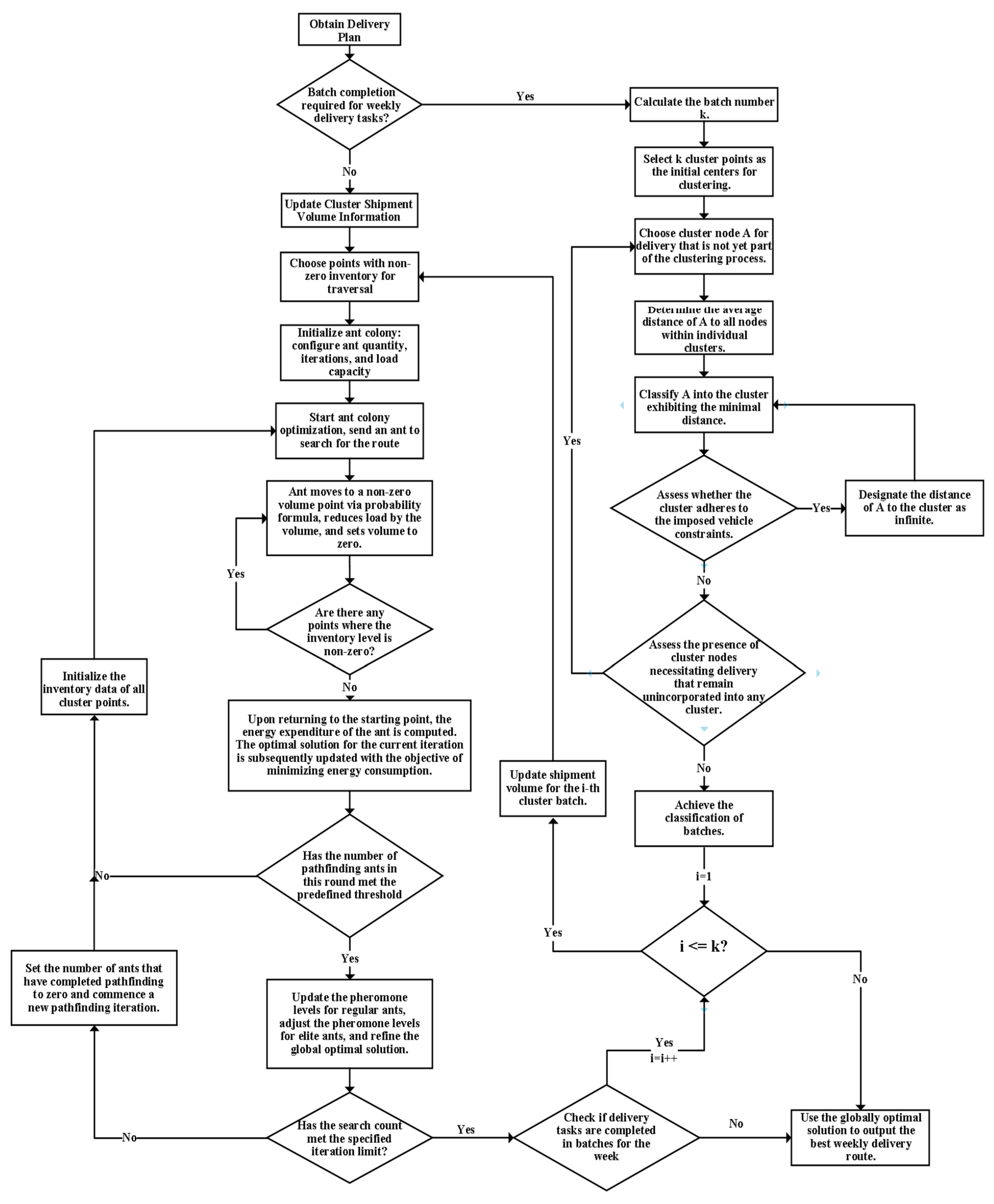
4.2.3. Steps to Improve the Ant Colony Algorithm

The improved ant colony algorithm has a faster iteration speed, closer distance processing to the real situation, and can deal with the problem of load, capacity, mileage, and other constraints, as well as solve the distribution route that minimizes carbon emissions. The steps of the optimized ant colony algorithm are shown in Figure 3, and the corresponding pseudo-code is shown in Appendix B.

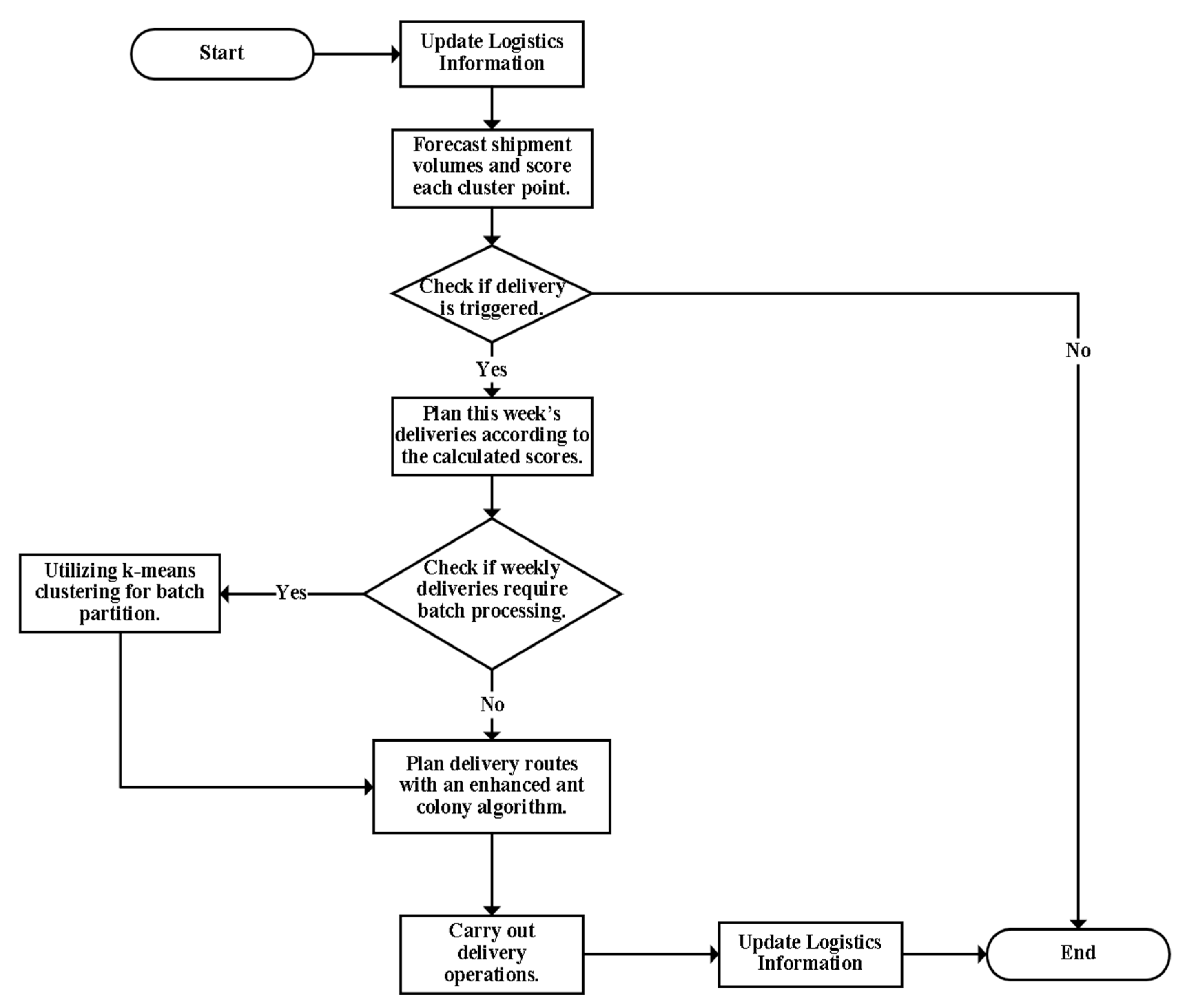
4.3. Flow of Optimized Model

The overall flow of the optimized model for the case of urban joint distribution of Company M is shown in Figure 4:

Compared with the original model, the optimized M company’s urban joint distribution model involves more planning, always focusing on the objective of reducing carbon emissions and reducing the enterprise’s carbon emissions and distribution costs while meeting the needs of downstream users.

5. Results

5.1. Instance Data and Parameters

In this chapter, the data of company M with more activities in 2 months and 9 weeks are selected for simulation. The default initial freight weight to be delivered is 0. After desensitization and cluster point integration, the data of the freight weight to be delivered in the first 4 weeks are shown in

Table 5. Logistics demand of each cluster point.

Serial Number	location	Week 1	Week 2	Week 3	Week 4
1	Yuanda Park and surrounding areas	10.2	11.9	11.1	12.8
2	Bajiajiayuan and surrounding areas	9.1	9.7	8.4	9.9
3	Beijing Foreign Studies University and surrounding areas	22.8	43.7	13.3	24.7
4	China Agricultural University and surrounding areas	12.4	9.0	5.7	7.9
5	Anxiangli and surrounding areas	13.9	13.1	11.3	9.6
6	China University of Geosciences and surrounding areas	85.1	74.5	101.1	98.4
7	Peony Garden Xili community and surrounding areas	11.2	5.1	7.9	4.1
8	Yilin homeland and surrounding areas	8.5	9.2	5.4	6.9
9	Anzhenli community and surrounding areas	7.1	10.7	10.7	11.6
10	Guoao village community and surrounding areas	0	17.7	12.6	11.9
11	Andedongli and surrounding areas	15.7	18.6	12.9	21.5
12	Huizhong Beili and surrounding areas	11.5	6.6	19.7	18.0
13	Beijing Normal University and surrounding areas	64.1	66.6	81.1	69.0
14	Huixin building and surrounding areas	8.3	7.1	4.8	8.3
15	Beiying community and its surrounding areas	12.0	14.7	17.5	24.8
16	Peking University and surrounding areas	107.9	81.8	117.8	70.7
17	Wanquan business garden and surrounding areas	10.2	11.2	15.8	11.2
18	Beijing Jiaotong University and surrounding areas	36.5	25.7	31.1	20.3
19	Beijing University of Aeronautics and Astronautics and surrounding areas	55.9	31.6	20.0	41.2
20	China University of political science and law and surrounding areas	22.7	12.4	13.4	15.5
21	Capital Institute of physical education and its surrounding areas	21.3	17.0	25.6	19.9
22	Renmin University of China and surrounding areas	14.9	12.9	16.8	11.9

. The freight weight information is counted in cluster points, and the freight weight is described in kg. The regions where there is no distribution demand are not counted. For convenience of description, the following will still be described in cluster points.

The important parameter settings involved in the example analysis in this paper are shown in

Table 6. Parameter setting.

Symbol	Meaning	Assignment
$W_g$	Delayed delivery stage: weight coefficient of reference value of cargo volume	0.1
$W_t$	Delayed delivery stage: weight coefficient of time reference value	1.0
$W_f$	Delayed delivery stage: weight coefficient of associated reference value	0.5
$a_j$	Delayed delivery stage: weight coefficient of the forecast value in week j	0.75, 0.5, 0.25
$\rho$	Path optimization stage: Volatilization Coefficient of pheromone concentration	0.5
$\alpha$	Path optimization stage: an important factor of pheromone	1.0
$\beta$	Route optimization stage: an important factor of visibility	2.0
$Q_{\tau }^{elite}$	Path optimization stage: the total amount of pheromones carried by elite ants	100
$Q_{\tau }^{ordinary}$	Path optimization stage: the total amount of pheromones carried by ordinary ants	50

:

The maximum load of the distribution vehicle is 400 kg, taking 360–400 kg as the floating range of the full load, and the mileage is calculated as 80 km. In terms of driving energy consumption, the energy consumption is calculated as 0.47 ah/km without load, 1.0 ah/km with 400 kg load, and the battery capacity is 60 ah. The maximum distribution mileage per week is calculated as 160 km.

The distance of some nodes in this case is shown in

Table 7. Node (partial) distance table.

Node Serial Number	0	1	2	3	4	5	6	7	8	9	10	11	12	13	14
0	0	129	18	100	41	76	48	81	43	119	58	124	74	96	91
1	129	0	123	29	120	129	97	102	146	126	145	97	163	79	150
2	18	123	0	94	23	58	30	63	25	101	40	106	56	78	73
3	100	29	94	0	91	100	68	73	117	97	116	68	134	50	121
4	41	120	23	91	0	35	23	40	26	78	25	83	43	55	50
5	76	129	58	100	35	0	32	27	33	43	18	48	34	50	21
6	48	97	30	68	23	32	0	33	49	71	48	76	66	48	53
7	81	102	63	73	40	27	33	0	44	38	43	43	61	23	48
8	43	146	25	117	26	33	49	44	0	76	15	81	31	67	48
9	119	126	101	97	78	43	71	38	76	0	61	29	45	47	28
10	58	145	40	116	25	18	48	43	15	61	0	66	18	66	33
11	124	97	106	68	83	48	76	43	81	29	66	0	66	28	53
12	74	163	56	134	43	34	66	61	31	45	18	66	0	84	17
13	96	79	78	50	55	50	48	23	67	47	66	28	84	0	71
14	91	150	73	121	50	21	53	48	48	28	33	53	17	71	0
15	77	88	59	59	36	41	29	14	58	42	57	47	75	19	62
16	60	69	54	42	51	60	32	65	77	103	76	108	94	80	81
17	95	34	89	25	86	95	63	68	112	92	111	91	129	63	116
18	87	50	73	29	70	79	47	52	96	76	95	47	113	29	100

, unit: 100 m.

5.2. Example Solution

5.2.1. Solution Steps

(1) Weekly distribution weight solution: use the scoring system to delay the distribution idea explained above and use the data of 2 months and 9 weeks with more activities of M company to solve the problem, so as to obtain weekly distribution planning, and then obtain the total weekly distribution and the freight weight to be distributed.

(2) Distribution grouping solution: use the k-means clustering method mentioned above to batch process weekly distribution operations that need to be divided into batches and obtain the batch results of the corresponding week.

(3) After obtaining the distribution scheme and batch results in the above two steps, the improved ant colony algorithm is used to solve the distribution route and obtain the final distribution route.

5.2.2. Final Distribution Route Solution

The solution of distribution route based on improved ant colony algorithm is shown in

Table 8. Distribution route table.

Time	Route	Total Road Length (km)	Energy Consumption (Ah)
Week 1	[0, 4, 6, 16, 22, 18, 20, 21, 19, 7, 5, 14, 0]	35.6	24.45
Week 2	[0, 16, 3, 18, 19, 13, 11, 10, 0]	35.6	24.87
Week 3	[0, 16, 17, 1, 3, 18, 20, 21, 19, 2, 0] [0, 6, 15, 13, 9, 12, 8, 0]	27.4 25.6	20.12 17.01
Week 4	[0, 6, 5, 11, 13, 15, 22, 1, 16, 0]	38.2	26.62
Week 5	[0, 2, 19, 21, 20, 18, 3, 1, 17, 22, 16, 0] [0, 4, 6, 5, 7, 15, 13, 11, 9, 14, 12, 10, 0]	29.4 33.2	20.82 21.44
Week 6	[0, 2, 8, 10, 12, 14, 9, 11, 13, 20, 18, 3, 1, 17, 22, 16, 6, 19, 21, 15, 7, 5, 4, 0]	52.4	39.78
Week 7	[0, 2, 4, 6, 19, 21, 22, 16, 17, 1, 3, 18, 20, 13, 11, 7, 5, 14, 12, 10, 8, 0]	49.2	34.44
Week 8	[0, 4, 7, 15, 21, 19, 6, 16, 22, 17, 1, 3, 18, 20, 13, 11, 7, 5, 14, 12, 10, 8, 0]	54.2	37.86
Week 9	[0, 2, 4, 6, 19, 21, 15, 7, 13, 20, 18, 3, 1, 22, 16, 12, 8, 0]	47	32.05

below.

5.3. Comparative Analysis

5.3.1. Comparison of Distribution Planning

The examples provided in this chapter are simulated, and the score method utilized in this study is delayed delivery as opposed to immediate distribution and full-load distribution.

Using the k-means clustering approach demonstrated in this article batch, immediate distribution is a weekly distribution in which all of the commodities are to be distributed this week, even if it requires numerous batches to finish the distribution operation.

Full-load distribution: plan distribution so that there is no empty load as much as feasible, and schedule it when the freight to be distributed may reach the full load or is close to the latest distribution time. The k-means clustering algorithm presented in this work is utilized for batching when several deliveries are needed. For these three types of deliveries, the final tabulation includes the number of deliveries, the number of cluster visits, the empty load rate, and the weight of deliveries. As shown in

Table 9. Distribution planning comparison table.

Method Name	Number of Distributions	Access to Cluster Points	Unladen Rate	Distribution Weight (kg)
Delayed delivery	11	139	6.6%	4111.3
Fully loaded distribution	10	151	0.2%	3992.5
Instant distribution	16	197	34.9%	4172.1

below.

From the standpoint of carbon emissions, the score system presented in this article can effectively reduce the number of deliveries, the rate of empty loads, save capacity, and reduce carbon emissions by approximately 20.4% when compared to immediate distribution; when compared to full-loaded distribution, it can effectively reduce the number of visits to the cluster points, which lowers the distribution mileage and reduces carbon emissions by approximately 7.9%.

5.3.2. Comparison of Route Optimization

The traditional ant colony algorithm with the objective of shortest route is used for route optimization, where the routes, total route lengths, and energy consumption are calculated and a table is produced, while maintaining the weekly distribution planning scheme that was obtained using the delayed delivery strategy. As shown in

Table 10. Shortest distribution route table.

Time	Route	Total Road Length (km)	Energy Consumption (Ah)
Week 1	[0, 4, 14, 5, 7, 19, 21, 20, 18, 22, 16, 6, 0]	34	28.39
Week 2	[0, 19, 16, 3, 18, 13, 11, 10, 0]	35.2	25.25
Week 3	[0, 16, 17, 1, 3, 18, 20, 21, 19, 2, 0] [0, 8, 12, 9, 13, 15, 6, 0]	27.4 25.6	20.12 21.08
Week 4	[0, 6, 5, 11, 13, 15, 22, 1, 16, 0]	38.2	26.62
Week 5	[0, 2, 19, 21, 20, 18, 3, 1, 17, 22, 16, 0] [0, 10, 12, 14, 9, 11, 13, 15, 7, 5, 6, 4, 0]	29.4 33.2	20.82 22.63
Week 6	[0, 2, 8, 10, 12, 14, 9, 11, 13, 20, 18, 3, 1, 17, 22, 16, 6, 19, 21, 15, 7, 5, 4, 0]	52.4	39.78
Week 7	[0, 2, 8, 10, 12, 14, 5, 7, 19, 21, 20, 13, 11, 18, 3, 1, 17, 22, 16, 6, 4, 0]	49.2	39.5
Week 8	[0, 8, 10, 12, 9, 11, 13, 15, 21, 18, 3, 1, 17, 22, 16, 6, 19, 7, 5, 4, 0]	52.2	40.26
Week 9	[0, 2, 8, 12, 4, 6, 19, 21, 15, 7, 13, 20, 18, 1, 3, 22, 16, 0]	43.8	32.99

below.

The improved ant colony method in this study has 7.2 km more overall route length than the traditional ant colony algorithm, but it uses 17.98 Ah less battery power, according to a comparison of the route optimization tables of the two ant colony algorithms. From a carbon emission standpoint, the optimization rate is 5.7%, the carbon emission is decreased by 1.29 kg, and the distribution cost stays the same.

5.4. Summary of Optimization Results

The optimized distribution plan and the carbon emission optimization effect in comparison to the conventional technique are produced following the example calculation in Section 5.2 and the method comparison analysis in Section 5.3.

A total of 11 distribution operations and 139 visits to cluster points are needed to finish the distribution tasks when combining the 9-week shipment data utilizing the co-distribution optimization scheme suggested in this article. The battery’s overall energy consumption is 299.46 Ah, and the distribution distance is 427.8 km. About 8.62 kg of standard coal must be burned, based on the current thermal efficiency of 18% of the coal furnace for burning lump coal, and 47.9 kg of standard coal must be burned if the battery’s energy consumption is converted into carbon emissions and coal consumption, which results in a total of 21.5 kg of CO₂ emissions.

In terms of the carbon emission optimization effect, when only considering distribution planning, the optimization range of the optimization scheme shown in this article is 20.4% and 7.9%, respectively, compared with instant distribution and full load distribution; When only considering the route optimization, the optimization scheme shown in this article achieves 5.7% compared with the traditional ant colony algorithm. Considering the two aspects together, the total optimization range of carbon emissions is about 33.5% compared with the original distribution mode of M company.

6. Conclusions

6.1. Summary

With global warming, carbon emissions have become a global problem. Globally, the proportion of carbon emissions from the logistics industry in total carbon emissions is also increasing, which has brought challenges to the logistics industry. Therefore, the necessity of reducing logistics carbon emissions has been widely acknowledged. In order to explore ways to reduce logistics carbon emissions, this article takes M company’s urban joint distribution as an example to study the reduction of carbon emissions from distribution operations. The following specific work has been performed:

(1) Formula derivation

The two primary factors influencing carbon emissions from distribution operations—transportation distance and load capacity of vehicles—are translated into kilogram kilometers of distribution vehicles, which are composed of three components: virtual load, vehicle weight, and vehicle load, using the formula for calculating carbon emissions from distribution operations. This gives us the article’s optimization direction, which aims to optimize the distribution route and lower the empty load rate.

(2) Establishment of the mathematical model

With the aim of reducing carbon emissions, a mathematical model of Company M’s urban joint distribution is developed, accounting for the limitations of distribution vehicle load, mileage, logistical time limit, and other factors. By optimizing the objective, it can lower carbon emissions, save distribution costs, and satisfy Company M’s logistics needs.

(3) Establishment of the scoring based delayed delivery model

A scoring based delayed delivery model was developed by combining the concept of delayed delivery. This model aims to reduce the empty load rate and achieve economies of scale to help reduce carbon emissions. By calculating scores for cluster points, it clarifies when to carry out distribution operations and which cluster points to carry out distribution operations for. This model enables M company to arrange fewer distribution batches, visit fewer cluster points, and reduce the total distribution mileage while meeting the same logistics needs.

(4) Improved ant colony Algorithm

The common methods of path optimization are analyzed and compared. The ant colony algorithm is selected as the method of path optimization in this article. The problems of traditional ant colony algorithms that cannot consider distribution energy consumption, cannot deal with load limitations and have slow iteration speeds are solved by using the introduction of minimum energy consumption, employing k-means clustering, and setting up elite ants, respectively, making it more suitable for solving the problem of M company’s urban joint distribution.

(5) Numerical simulation

Numerical simulations are implemented using C and Python, the specific software and version are shown in

Table A1. Relevant software and environment versions programmed in this article.

Library/Environment/Software	Version	Library/Environment/Software	Version
Dev-C++	6.3	sympy	1.6.2
pandas	1.4.2	SQLAlchemy	1.3.20
numpy	1.22.4	Pillow	8.0.1
python-dateutil	2.8.1	matplotlib	3.5.1
scipy	1.7.3	openpyxl	3.0.5

in Appendix A. The comparative experiments are carried out for the score based delayed delivery and the improved ant colony algorithm. Compared with the current distribution mode of M company, the optimization range is 20.4% and 5.7%, respectively, and the comprehensive optimization range is 33.5%, which proves that the model proposed in this article can reduce carbon emissions.

6.2. Discussion

Influenced by individual academic ability, research facilities, enterprise data, and other factors, the research in this article still has room for further expansion in the following aspects:

(1) Economic elements that are relatively biased in cost computation, such as out-of-stock costs, communication costs, time costs, depreciation costs, and brand benefits, are not taken into account in this work. In order to reduce carbon emissions while regulating costs from a broad perspective, future research can depict carbon emissions as costs that encompass a larger spectrum of the company’s operations.

(2) This model only considers the general scenarios, the robustness of the model in extreme scenarios, such as peak demand surge, is not discussed. In the future, we should strengthen the research of the model in extreme scenarios and enhance the universality of the model.

(3) The results of future examples in this article can be compared with the results of other heuristic algorithms, so as to highlight the practical significance of the optimization model in this article.

References

1. Babagolzadeh, M.; Shrestha, A.; Abbasi, B.; Zhang, Y.; Woodhead, A.; Zhang, A. Sustainable cold supply chain management under demand uncertainty and carbon tax regulation. Transp. Res. Part D Transp. Environ. 2020, 80, 102245. [Google Scholar] [CrossRef]
2. Cheng, L.D. Vehicle Routing Problem with Fuzzy Timewindows Considering with Carbon Emission. Ph.D. Thesis, Zhejiang University of Technology, Hangzhou, China, 2018. [Google Scholar]
3. Lu, M.M. Research on Multi-Objective Path Planning Problem of Cold Chain Logistics with Carbon Emission and Fuzzy Time Windows. Ph.D. Thesis, Shanghai Ocean University, Shanghai, China, 2020. [Google Scholar]
4. Dong, J.M. Research on the Vehicle Routing Optimization of Convenience Stores Considering Carbon Emissions and Multi Distribution Centers. Ph.D. Thesis, Nanjing University, Nanjing, China, 2021. [Google Scholar]
5. Guo, Z.; Zhang, X.; Zheng, Y.; Rao, R. Exploring the impacts of a carbon tax on the Chinese economy using a CGE model with a detailed disaggregation of energy industrys. Energy Econ. 2014, 45, 455–462. [Google Scholar] [CrossRef]
6. Hariga, M.; As’ad, R.; Shamayleh, A. Integrated economic and environmental models for a multi stage cold supply chain under carbon tax regulation. J. Clean. Prod. 2017, 166, 1357–1371. [Google Scholar] [CrossRef]
7. Bai, Q.; Gong, Y.; Jin, M.; Xu, X. Effects of carbon emission reduction on supply chain coordination with vendor-managed deteriorating product inventory. Int. J. Prod. Econ. 2019, 208, 83–99. [Google Scholar] [CrossRef]
8. Jauhari, W.A.; Cahaya Sakti, C.T.; Hisjam, M.; Hishamuddin, H. A sustainable circular economic supply chain model with green production, delays in payment, and carbon tax regulation. J. Clean. Prod. 2025, 495, 145008. [Google Scholar] [CrossRef]
9. Shimizu, Y.; Sakaguchi, T.; Shimada, H. Multi-objective optimization for creating a low-carbon logistics system through community-based action. J. Adv. Mech. Des. Syst. Manuf. 2015, 9, JAMDSM0063. [Google Scholar] [CrossRef]
10. Liu, F.; Chen, W.-L.; Fang, D.-B. Optimal coordination strategy of dynamic supply chain based on cooperative stochastic differential game model under uncertain conditions. Appl. Soft Comput. 2017, 56, 669–683. [Google Scholar] [CrossRef]
11. Zhang, X.; Jin, F.-Y.; Yuan, X.-M.; Zhang, H.-Y. Low-Carbon Multimodal Transportation Path Optimization under Dual Uncertainty of Demand and Time. Sustainability 2021, 13, 8180. [Google Scholar] [CrossRef]
12. Liu, Z.; Niu, Y.; Guo, C.; Jia, S. A Vehicle Routing optimization Model for Community Group Buying Considering Carbon Emissions and Total Distribution Costs. Energies 2023, 16, 931. [Google Scholar] [CrossRef]
13. Ma, L.; Li, M. Research on a Joint Distribution Vehicle Routing Problem Considering Simultaneous Pick-Up and Delivery under the Background of Carbon Trading. Sustainability 2024, 16, 1698. [Google Scholar] [CrossRef]
14. Dantzig, G.B.; Ramser, J.H. The truck dispatching problem. Manag. Sci. 1959, 6, 80–91. [Google Scholar] [CrossRef]
15. Cheng, N.; She, L.; Chen, D. Electric Vehicle Charging Scheduling Optimization Method Based on Improved Ant Colony. J. Phys. Conf. Ser. 2023, 2418, 012112. [Google Scholar] [CrossRef]
16. Gao, P.; Zhou, L.; Zhao, X.; Shao, B. Research on ship collision avoidance path planning based on modified potential field ant colony algorithm. Ocean Coast. Manag. 2023, 235, 106482. [Google Scholar] [CrossRef]
17. Li, E.; Qi, K. Ant Colony Algorithm for Path Planning Based on Grid Feature Point Extraction. J. Shanghai Jiaotong Univ. (Sci.) 2023, 28, 86–99. [Google Scholar] [CrossRef]
18. Luo, Q.; Wang, H.B.; Zheng, Y.; He, J.C. Research on path planning of mobile robot based on improved ant colony algorithm. Neural Comput. Appl. 2020, 32, 1555–1566. [Google Scholar] [CrossRef]
19. Liu, J.H.; Yang, J.G.; Liu, H.P.; Tian, X.J.; Gao, M. An improved ant colony algorithm for robot path planning. Soft Comput. 2017, 21, 5829–5839. [Google Scholar] [CrossRef]
20. Wei, L.; Zhang, Z.; Zhang, D.; Leung, S.C.H. A simulated annealing algorithm for the capacitated vehicle routing problem with two-dimensional loading constraints. Eur. J. Oper. Res. 2018, 265, 843–859. [Google Scholar] [CrossRef]
21. Li, G.; Li, J. An Improved Tabu Search Algorithm for the Stochastic Vehicle Routing Problem With Soft Time Windows. IEEE Access 2020, 8, 158115–158124. [Google Scholar] [CrossRef]
22. Xu, J.; Han, Y.; Liu, J.; Pan, N.; Yin, S.; Liang, W.; Han, W.; Lin, C. Investigation of the joint Automated mobile loading systems Two-Stage vehicle routing problem under the consideration of Supply-Demand Imbalance, fair Efficiency, and demand uncertainty. Comput. Oper. Res. 2025, 181, 107108. [Google Scholar] [CrossRef]
23. Zhen, L.; Ma, C.; Wang, K.; Xiao, L.; Zhang, W. Multi-depot multi-trip vehicle routing problem with time windows and release dates. Transp. Res. Part E Logist. Transp. Rev. 2020, 135, 101866. [Google Scholar] [CrossRef]
24. Zhang, S.; Gajpal, Y.; Appadoo, S.S.; Abdulkader, M.M.S. Electric vehicle routing problem with recharging stations for minimizing energy consumption. Int. J. Prod. Econ. 2018, 203, 404–413. [Google Scholar] [CrossRef]
25. Xiong, H.; Xu, Y.; Yan, H.; Guo, H.; Zhang, C. Optimizing electric vehicle routing under traffic congestion: A comprehensive energy consumption model considering drivetrain losses. Comput. Oper. Res. 2024, 168, 106710. [Google Scholar] [CrossRef]
26. Jiang, Y.; Hu, W.; Gu, W.; Yu, Y.; Xu, M. A multi-mode hybrid electric vehicle routing problem with time windows. Transp. Res. Part E Logist. Transp. Rev. 2025, 195, 103976. [Google Scholar] [CrossRef]
27. Boyack, J.; Choi, J.B.; Jeong, J.; Park, H.; Kim, S. LogPath: Log data based energy consumption analysis enabling electric vehicle path optimization. Transp. Res. Part D Transp. Environ. 2024, 135, 104387. [Google Scholar] [CrossRef]
28. Gao, C.H. Study on Optimization of Low-Carbon Distribution Routing of T Company. Ph.D. Thesis, University of Jinan, Shandong, China, 2022. [Google Scholar]
29. Ottmar, R.D. Wildland fire emissions, carbon, and climate: Modeling fuel consumption. For. Ecol. Manag. 2014, 317, 41–50. [Google Scholar] [CrossRef]
30. Chen, Y.S.; Ma, J.Q.; Ding, Z.S.; Chen, H. Research on life cycle energy conservation and emission reduction performance assessment of power system for pure electric vehicle. Mach. Electron. 2018, 36, 20–23. [Google Scholar]
31. Liu, L.L.; Liu, T.L.; Jin, X.X. The discussion of calculation method of electric vehicle carbon emission and tracking evaluation. Intern. Combust. Engine Parts 2022, 196–198. [Google Scholar] [CrossRef]
32. Tang, Y.Y.; Mao, B.H.; Zhou, Q.; Gao, Q.Q. Impact analysis on carbon emission factor in operations of electric vehicle. Transp. Energy Conserv. Environ. Prot. 2022, 18, 17–22. [Google Scholar]
33. Xiao, Y.; Zhao, Q.; Kaku, I.; Xu, Y. Development of a fuel consumption optimization model for the capacitated vehicle routing problem. Comput. Oper. Res. 2012, 39, 1419–1431. [Google Scholar] [CrossRef]
34. Zhou, Y.; Wang, D.P.; Zhao, Y. Study on the CO₂ emission evaluation of the provincial logistics operation and low-carbon strategy in china. China Popul. Resour. Environ. 2011, 21, 81–87. [Google Scholar]
35. Xue, J.M.; Sun, A.R. Study on logistics service quality evaluation of takeout platform based on SERVPERF Model. J. Hebei Univ. Sci. Technol. (Soc. Sci.) 2021, 21, 35–43. [Google Scholar]
36. De Livera, A.M.; Hyndman, R.J.; Snyder, R.D. Forecasting Time Series With Complex Seasonal Patterns Using Exponential Smoothing. J. Am. Stat. Assoc. 2011, 106, 1513–1527. [Google Scholar] [CrossRef]
37. Wang, Y.F. Implementation of multiple vehicle routing optimization system based on ant colony clustering algorithm. J. Hubei Univ. Natl. (Nat. Sci. Ed.) 2015, 33, 200–204+209. [Google Scholar]
Figure 1. Schematic diagram of distribution vehicle power consumption.
Sustainability 17 04602 g001
Figure 2. Example time series forecasting Chart.
Sustainability 17 04602 g002
Figure 3. Schematic diagram of the steps of the improved ant colony algorithm.
Sustainability 17 04602 g003
Figure 4. Schematic diagram of the optimized joint distribution process.
Sustainability 17 04602 g004