
Nonlinear Influence of Urban Environment on Dockless Shared Bicycle Travel Patterns


Abstract
1. Introduction
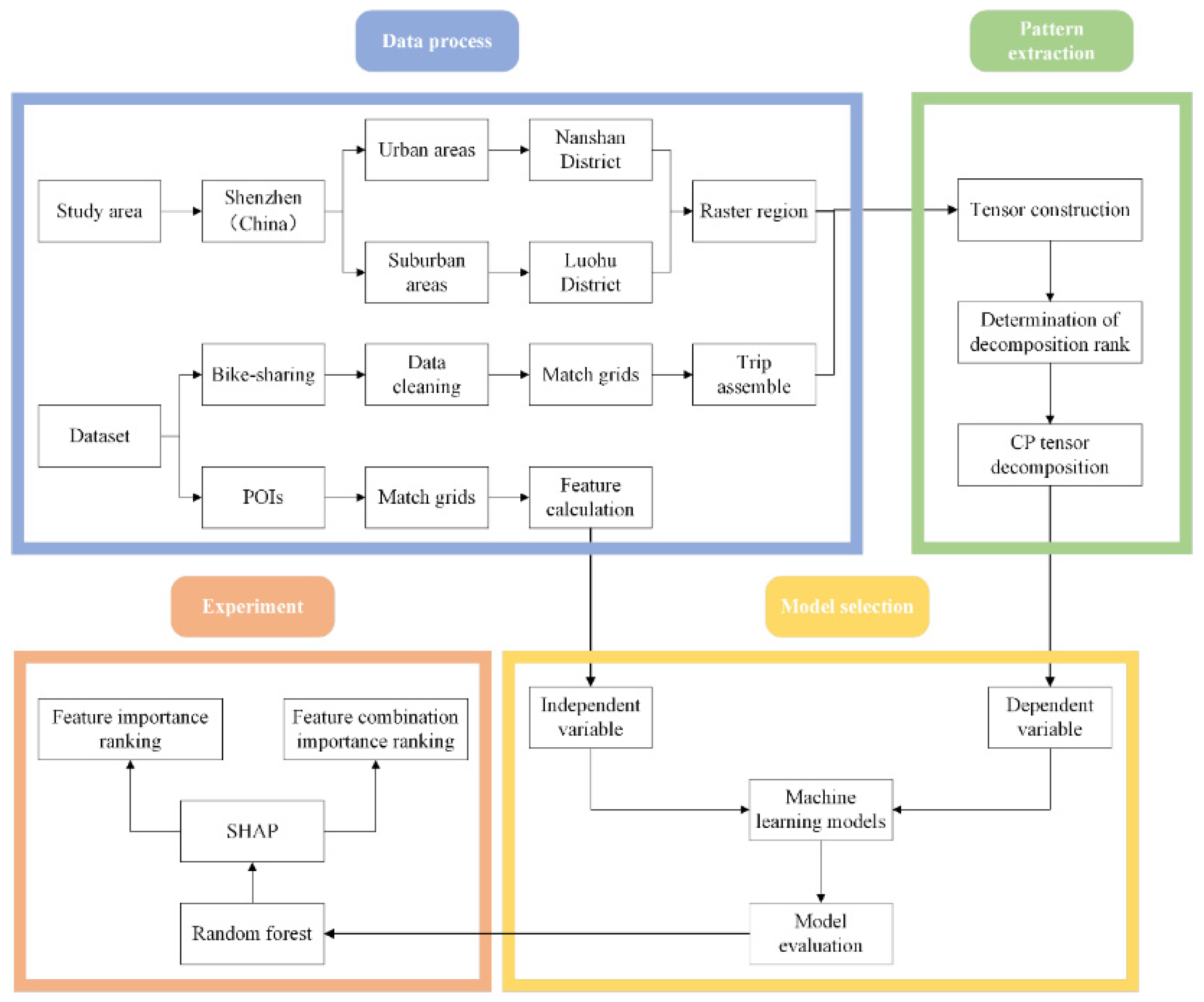
2. Methodology
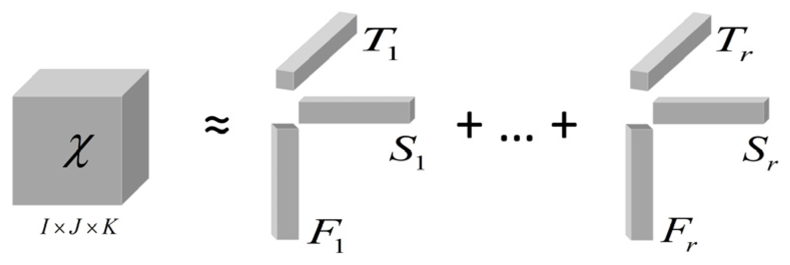
2.1. Tensor Decomposition
2.2. Prediction Model and Feature Importance Assessment
3. Data Preparation
3.1. Data Sources
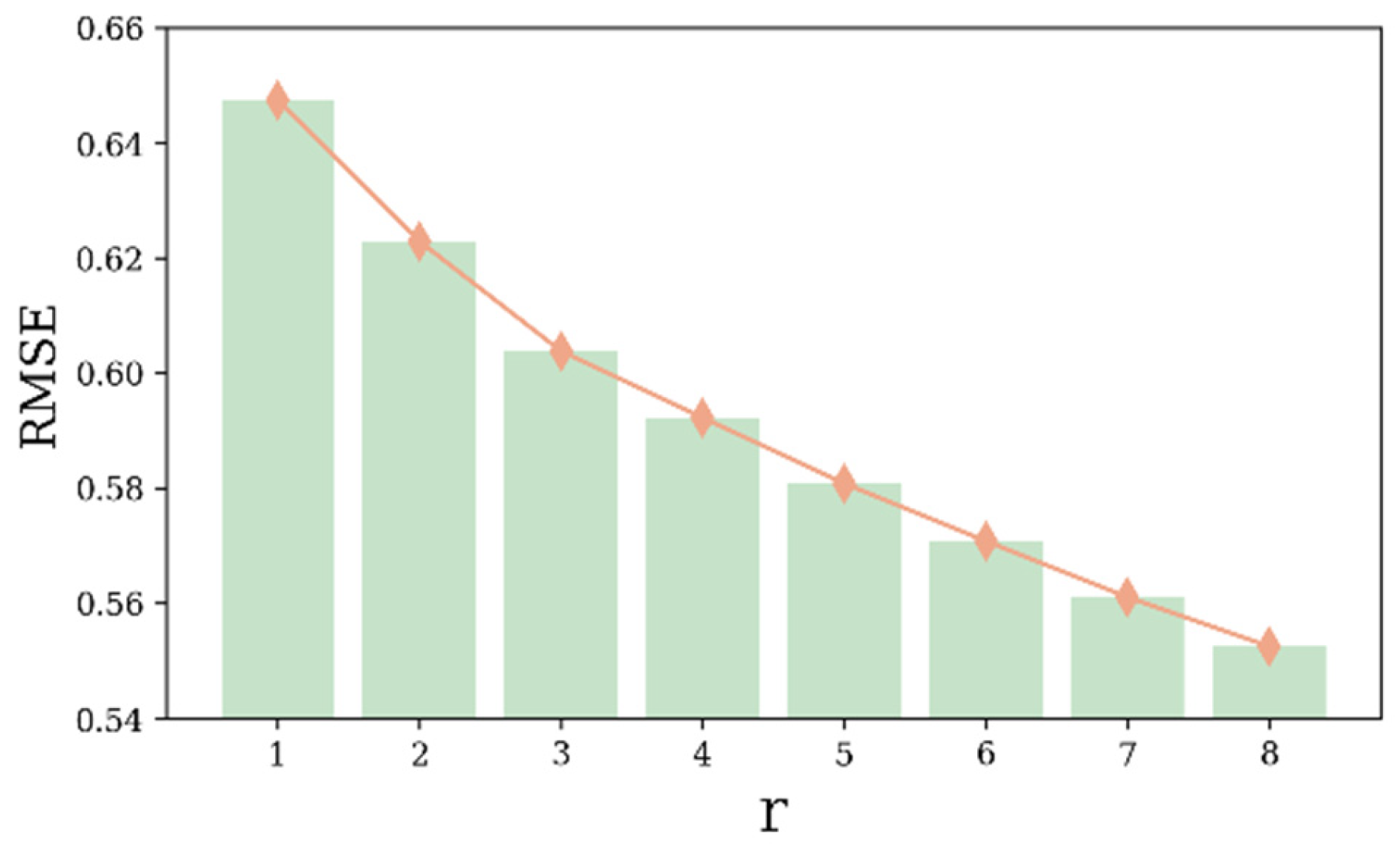
3.2. Tensor Construction and Determination of Decomposition Rank
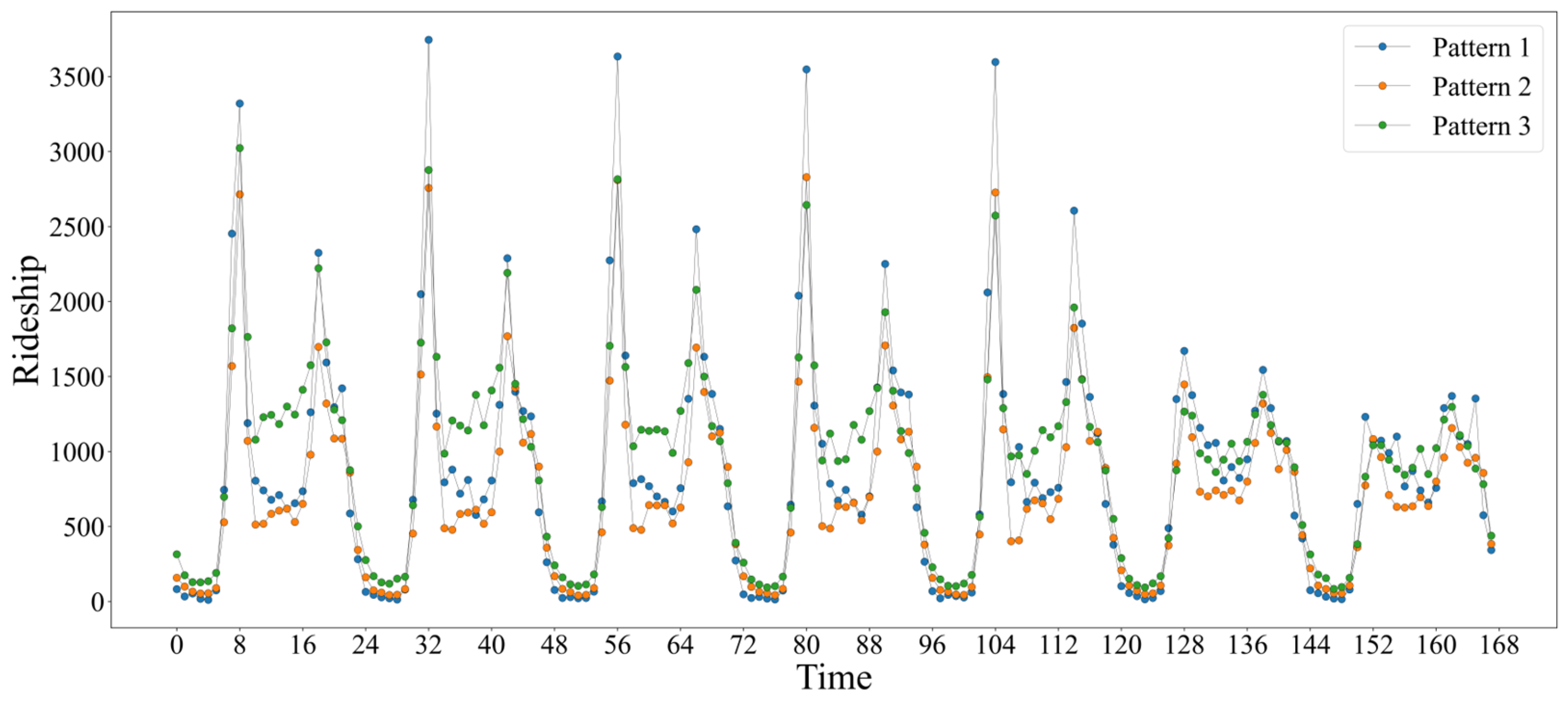
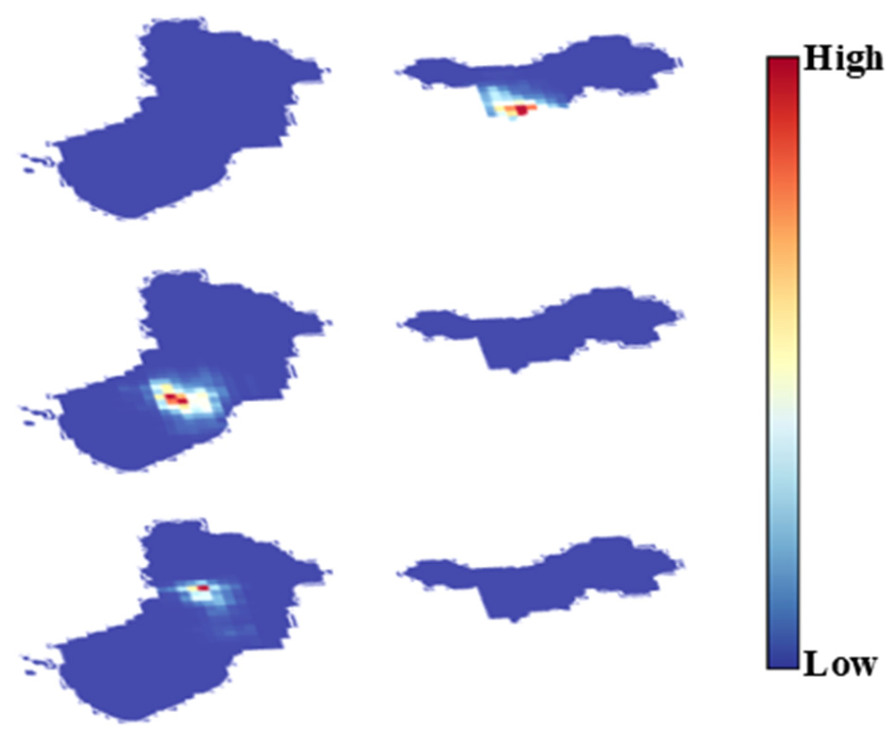
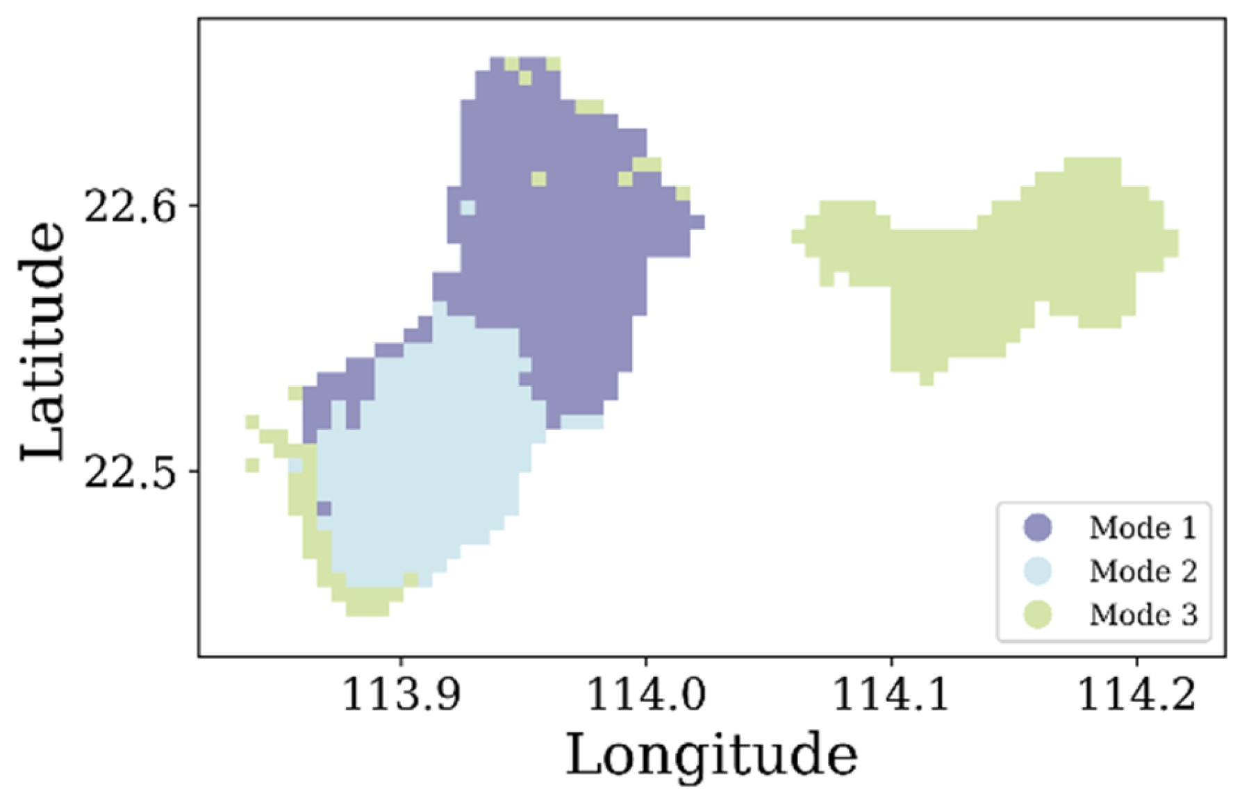
3.3. Determination of Travel Patterns
4. Experiments and Results
4.1. Model Training and Validation
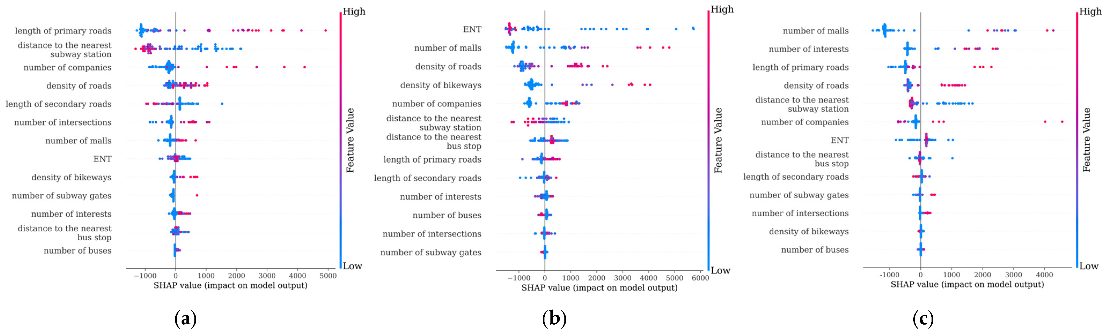
4.2. Importance Analysis of Features
4.3. Importance Analysis of Feature Combinations
5. Conclusions
- (1)
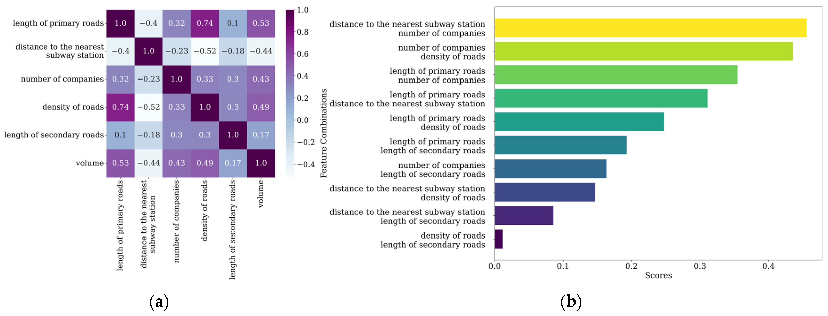
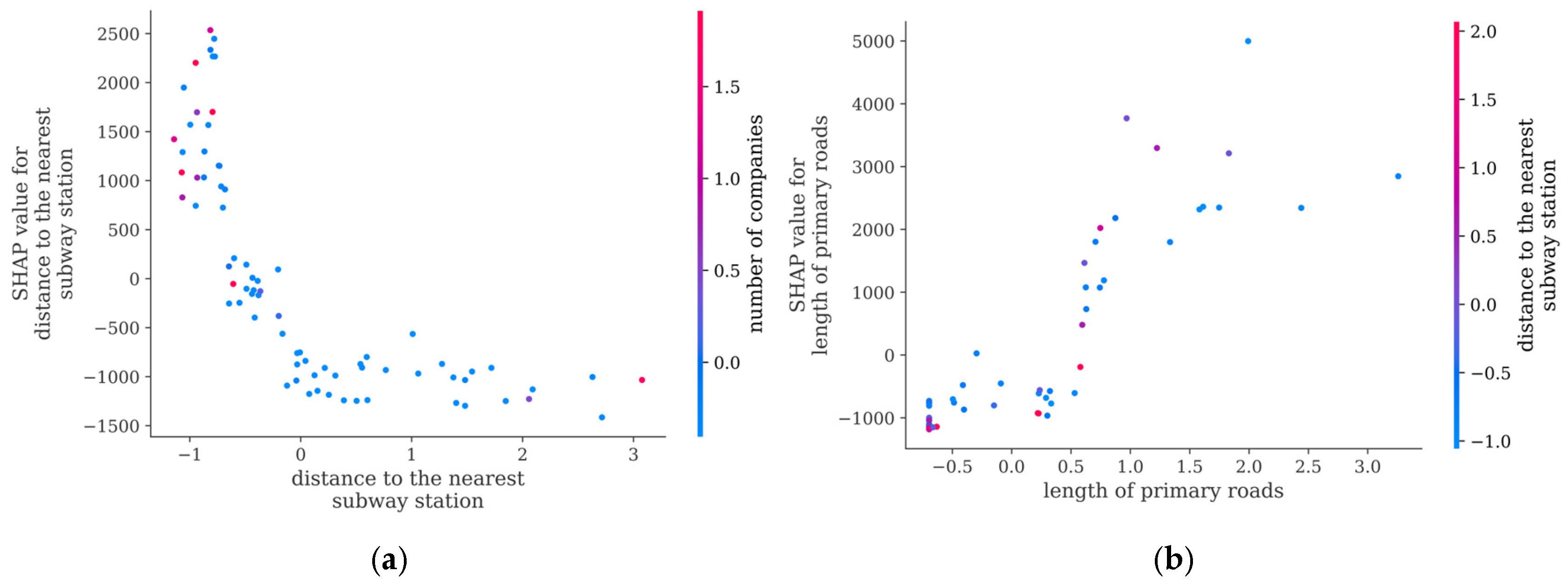
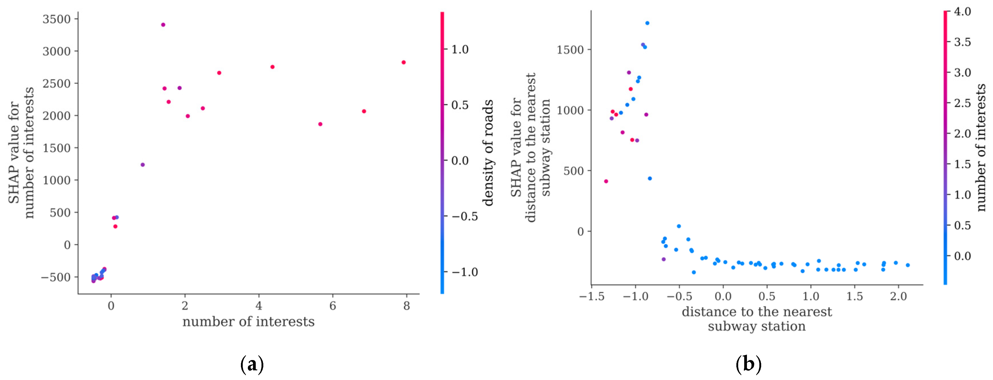
- For the peak-high traffic pattern, factors such as the length of the primary roads and distance to the nearest subway station have a significant impact. It is recommended to increase the number of shared bikes around major roads and near subway stations, while also constructing bike lanes to enhance convenience and safety. Additionally, attention should be given to the large demand for bikes generated by commuting. For example, travel is concentrated in the northern part of Nanshan District, leading to a high volume of trips during peak hours and little usage during off-peak hours. This requires management departments to make targeted bike-sharing adjustments to avoid situations where bikes are unavailable during peak hours and not used during off-peak hours.
- (2)
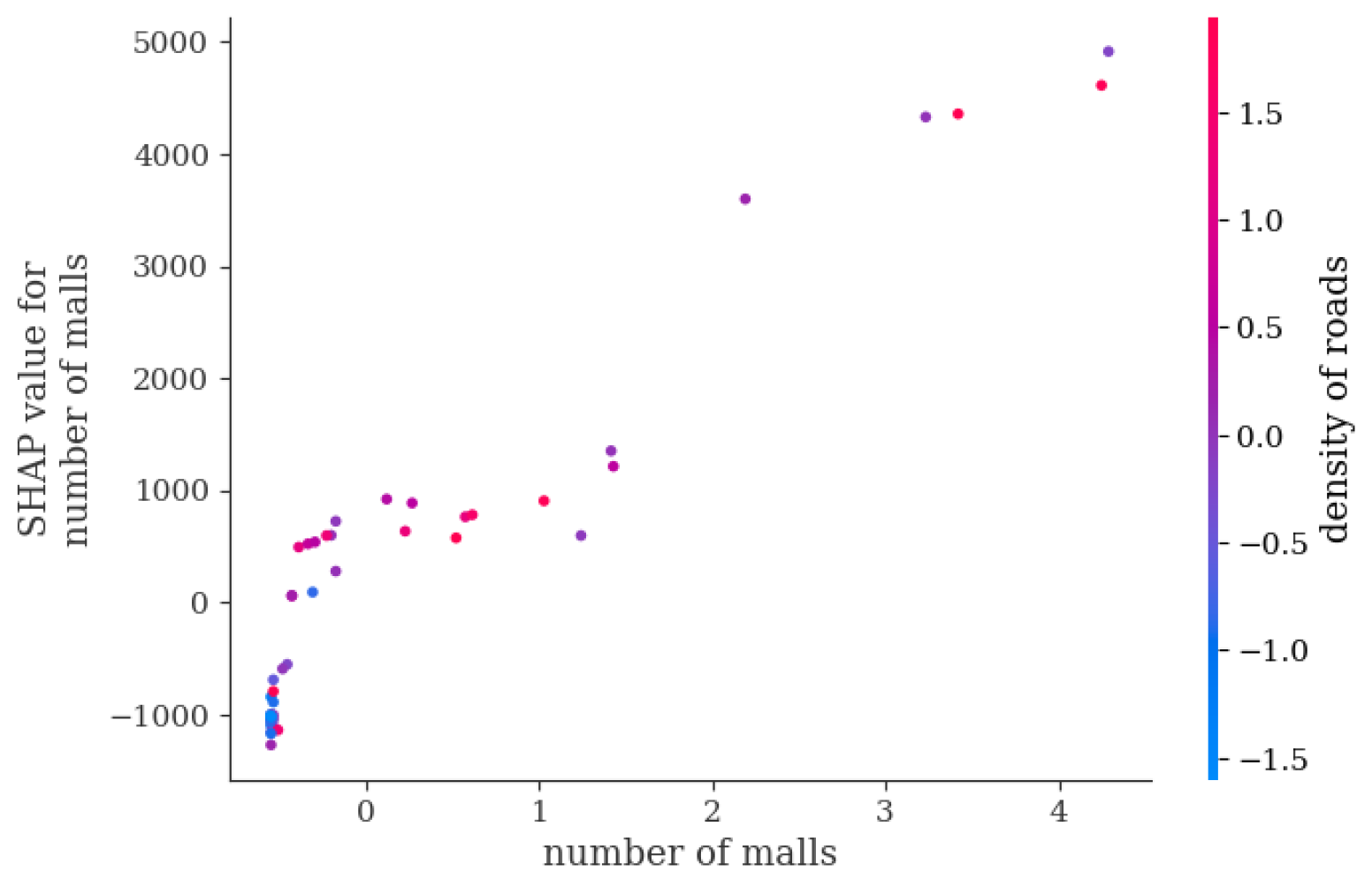
- For the steady traffic pattern, areas such as dedicated commercial districts, residential areas, and office areas are more attractive for bike-sharing usage. It is recommended to increase bike-sharing availability in areas with single-use land and clear demand while ensuring an adequate supply near places like shopping malls to meet user needs. For example, in the southern part of Nanshan District, during peak hours, attention should be given to the timely dispatch of shared bikes in these areas, with consideration of commuting as the primary purpose.
- (3)
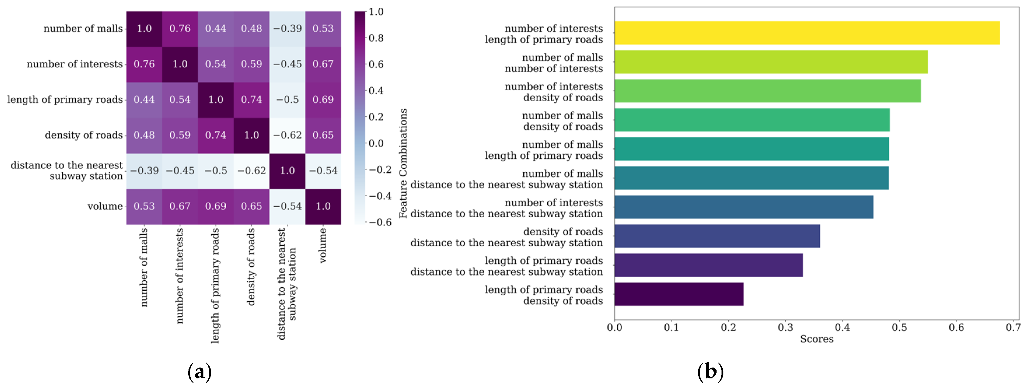
- For the off-peak high traffic pattern, scenes such as tourist interests and shopping malls generate more shared bike trips. It is recommended to deploy more shared bikes in these areas while also paying attention to the construction of road infrastructure. It is advised not to blindly increase the number of interests in urban planning to avoid suppressing bike-sharing use due to exceeding a certain threshold. For example, in Luohu District, trips are relatively dispersed. There is a high demand for bikes during peak hours, and considerable usage occurs during off-peak hours. Management departments should adopt more proactive dispatch strategies, responding more frequently and promptly to user needs to maintain the availability and efficiency of bike-sharing services.
Author Contributions
Funding
Institutional Review Board Statement
Informed Consent Statement
Data Availability Statement
Conflicts of Interest
Abbreviations
| POI | Points of interest |
| OD | Origin-destination |
| CP | CANDECOMP/PARAFAC |
| RF | Random forest |
| SHAP | Shapley additive explanations |
References
- Jiang, J.A.; Chen, S.L. Exploring the pathways of achieving carbon peaking and carbon neutrality targets in the provinces of the Yellow River basin of China. Sustainability 2024, 16, 6553. [Google Scholar] [CrossRef]
- Rimoldi, A.; Cenedese, C.; Padoan, A.; Dörfler, F.; Lygeros, J. Urban traffic congestion control: A DeePC change. In Proceedings of the 2024 European Control Conference, Stockholm, Sweden, 25–28 June 2024. [Google Scholar] [CrossRef]
- Tan, X.Y.; Zhu, X.L.; Li, Q.; Li, L.N.; Chen, J. Tidal phenomenon of the dockless bike-sharing system and its causes: The case of Beijing. Int. J. Sustain. Transp. 2022, 16, 287–300. [Google Scholar] [CrossRef]
- Figliozzi, M.; Tipagornwong, C. Impact of last mile parking availability on commercial vehicle costs and operations. Supply Chain Forum 2017, 18, 60–68. [Google Scholar] [CrossRef]
- Cui, Y.F.; Lv, W.F.; Wang, Q.; Du, B.W. Usage demand forecast and quantity recommendation for urban shared bicycles. In Proceedings of the 2018 International Conference on Cyber-Enabled Distributed Computing and Knowledge Discovery, Zhengzhou, China, 18–20 October 2018. [Google Scholar] [CrossRef]
- Dong, X.Y.; Zhang, B.; Wang, Z.H. Impact of land use on bike-sharing travel patterns: Evidence from large scale data analysis in China. Land Use Policy 2023, 133, 106852. [Google Scholar] [CrossRef]
- Wang, B.; Vu, H.L.; Kim, I.; Cai, C. Short-term traffic flow prediction in bike-sharing networks. J. Intell. Transport. Syst. 2022, 26, 461–475. [Google Scholar] [CrossRef]
- Du, M.Y.; Cheng, L. Better understanding the characteristics and influential factors of different travel patterns in free-floating bike sharing: Evidence from Nanjing, China. Sustainability 2018, 10, 1244. [Google Scholar] [CrossRef]
- Xing, Y.Y.; Wang, K.; Lu, J.J. Exploring travel patterns and trip purposes of dockless bike-sharing by analyzing massive bike-sharing data in Shanghai, China. J. Transp. Geogr. 2020, 87, 102787. [Google Scholar] [CrossRef]
- Kou, Z.Y.; Cai, H. Understanding bike sharing travel patterns: An analysis of trip data from eight cities. Phys. A 2019, 515, 785–797. [Google Scholar] [CrossRef]
- Li, Q.M.; Xu, W.P. The impact of COVID-19 on bike-sharing travel pattern and flow structure: Evidence from Wuhan. Camb. J. Reg. Econ. Soc. 2022, 15, 477–494. [Google Scholar] [CrossRef]
- Ma, J.Z.; Zheng, C.J.; Yu, M.; Shen, J.X.; Zhang, H.Y.; Wang, Y.Y. The analysis of spatio-temporal characteristics and determinants of dockless bike-sharing and metro integration. Transp. Lett. 2024, 16, 182–195. [Google Scholar] [CrossRef]
- Wang, F.Y.; Yin, C.Y.; Chang, X.M.; Zhang, X.Y.; He, Z.B. Exploring the relationship between built environment and bike-sharing demand: Does the trip length matter? Transp. Plan. Technol. 2024. [Google Scholar] [CrossRef]
- Quan, Y.F.; Wu, X.; Zhu, Z.J.; Liu, C.Y. Origin-destination spatial-temporal patterns of dockless shared bikes based on shopping activities and its application in urban planning: The case of Nanjing. Systems 2024, 12, 506. [Google Scholar] [CrossRef]
- Wang, F.Y.; Omar, S.; Wu, Y.C.; Zhang, X.Y.; He, J. Analysis of bike-sharing travel behavior using multi-day OD trip data. In Proceedings of the 23rd Joint COTA International Conference of Transportation Professionals, Beijing, China, 15–17 July 2023. [Google Scholar] [CrossRef]
- Peng, C.B.; Jin, X.G.; Wong, K.C.; Shi, M.X.; Liò, P. Collective human mobility pattern from taxi trips in urban area. PLoS ONE 2012, 7, e34487. [Google Scholar] [CrossRef]
- Li, Q.M.; Zhang, E.J.; Luca, D.; Fuerst, F. The travel pattern difference in dockless micro-mobility: Shared e-bikes versus shared bikes. Transport. Res. Part D Transport. Environ. 2024, 130, 104179. [Google Scholar] [CrossRef]
- Dong, J.; Chen, B.; He, L.; Ai, C.; Zhang, F.; Guo, D.; Qiu, X. A spatio-temporal flow model of urban dockless shared bikes based on points of interest clustering. ISPRS Int. J. Geo-Inf. 2019, 8, 345. [Google Scholar] [CrossRef]
- Chen, G.Y.; Wei, Z.C. Exploring the impacts of built environment on bike-sharing trips on weekends: The case of Guangzhou. Int. J. Sustain. Transp. 2024, 18, 315–327. [Google Scholar] [CrossRef]
- Ethier, B.G.; Wilson, J.S.; Camhi, S.M.; Shi, L.; Troped, P.J. An analysis of built environment characteristics in daily activity spaces and associations with bike share use. Travel Behav. Soc. 2024, 37, 100850. [Google Scholar] [CrossRef]
- Song, Y.C.; Luo, K.; Shi, Z.Y.; Zhang, L.; Shen, Y.G.; Tong, H.Y.; Torrao, G. Nonlinear influence and interaction effect on the imbalance of metro-oriented dockless bike-sharing system. Sustainability 2024, 16, 349. [Google Scholar] [CrossRef]
- Li, Z.T.; Shang, Y.Z.; Zhao, G.W.; Yang, M.Z. Exploring the multiscale relationship between the built environment and the metro-oriented dockless bike-sharing usage. Int. J. Environ. Res. Public Health 2022, 19, 2323. [Google Scholar] [CrossRef]
- Yang, H.T.; Zheng, R.; Li, X.; Huo, J.H.; Yang, L.C.; Zhu, T. Nonlinear and threshold effects of the built environment on e-scooter sharing ridership. J. Transp. Geogr. 2022, 104, 103453. [Google Scholar] [CrossRef]
- Zhuang, C.G.; Li, S.Y.; Tan, Z.Z.; Feng, G.; Wu, Z.F. Nonlinear and threshold effects of traffic condition and built environment on dockless bike sharing at street level. J. Transp. Geogr. 2022, 102, 103375. [Google Scholar] [CrossRef]
- Zhang, Y.; Thomas, T.; Brussel, M.; Maarseveen, M.V. Exploring the impact of built environment factors on the use of public bikes at bike stations: Case study in Zhongshan, China. J. Transp. Geogr. 2017, 58, 59–70. [Google Scholar] [CrossRef]
- Guo, Y.Y.; He, S.Y. Built environment effects on the integration of dockless bike-sharing and the metro. Transport. Res. Part D Transport. Environ. 2020, 83, 102335. [Google Scholar] [CrossRef]
- Silvestri, F.; Babaei, S.H.; Coppola, P. Improving urban cyclability and perceived bikeability: A decision support system for the city of Milan, Italy. Sustainability 2024, 16, 8188. [Google Scholar] [CrossRef]
- Coppola, P.; Silvestri, F. Gender inequality in safety and security perceptions in railway stations. Sustainability 2021, 13, 4007. [Google Scholar] [CrossRef]
- Villarrasa-Sapiña, I.; Toca-Herrera, J.L.; Pellicer-Chenoll, M.; Taczanowska, K.; Rueda, P.; Devís-Devís, J. Effects of meteorology on bike-sharing: Cases of 13 cities using non-linear analyses. Cities 2024, 155, 105457. [Google Scholar] [CrossRef]
- Kolda, T.G.; Bader, B.W. Tensor decompositions and applications. SIAM Rev. 2009, 51, 455–500. [Google Scholar] [CrossRef]
- Tang, H.; Fei, S.X.; Shi, X.Y. Revealing travel patterns from dockless bike-sharing data based on tensor decomposition. In Proceedings of the 12th International Symposium on Visual Information Communication and Interaction, Shanghai, China, 20 September 2019. [Google Scholar] [CrossRef]
- Lespinats, S.; Colange, B.; Dutykh, D. Nonlinear Dimensionality Reduction Techniques: A Data Structure Preservation Approach; Springer International Publishing: Cham, Switzerland, 2022. [Google Scholar] [CrossRef]
- Phan, A.H.; Tichavský, P.; Cichocki, A. Deflation method for CANDECOMP/PARAFAC tensor decomposition. In Proceedings of the 2014 IEEE International Conference on Acoustics, Speech and Signal Processing, Florence, Italy, 4–9 May 2014. [Google Scholar] [CrossRef]
- Hayashi, K.; Kishimoto, K.; Shimbo, M. Binarized embeddings for fast, space-efficient knowledge graph completion. IEEE Trans. Knowl. Data Eng. 2023, 35, 141–153. [Google Scholar] [CrossRef]
- Tang, J.J.; Wang, X.L.; Zong, F.; Hu, Z. Uncovering spatio-temporal travel patterns using a tensor-based model from metro smart card data in Shenzhen, China. Sustainability 2020, 12, 1475. [Google Scholar] [CrossRef]
- Rigatti, S.J. Random forest. J. Insur. Med. 2017, 47, 31–39. [Google Scholar] [CrossRef]
- Slack, D.; Hilgard, S.; Jia, E.; Singh, S.; Lakkaraju, H. Fooling lime and SHAP: Adversarial attacks on post hoc explanation methods. In Proceedings of the 3rd AAAI/ACM Conference on AI, Ethics, and Society, New York, NY, USA, 7–8 February 2020. [Google Scholar] [CrossRef]
- Choi, J.E.; Shin, J.W.; Shin, D.W. Vector SHAP values for machine learning time series forecasting. J. Forecast. 2025, 44, 635–645. [Google Scholar] [CrossRef]
- Gao, F.; Li, S.Y.; Tan, Z.Z.; Wu, Z.F.; Zhang, X.M.; Huang, G.P.; Huang, Z.W. Understanding the modifiable areal unit problem in dockless bike sharing usage and exploring the interactive effects of built environment factors. Int. J. Geogr. Inf. Sci. 2021, 35, 1905–1925. [Google Scholar] [CrossRef]
- Wang, J.Y.; Wu, J.J.; Wang, Z.; Gao, F.; Xiong, Z. Understanding urban dynamics via context-aware tensor factorization with neighboring regularization. IEEE Trans. Knowl. Data Eng. 2019, 32, 2269–2283. [Google Scholar] [CrossRef]
- Hamka, M.; Ramdhoni, N. K-means cluster optimization for potentiality student grouping using elbow method. In Proceedings of the 3rd International Conference on Engineering and Applied Sciences, Purwokerto, Indonesia, 26 July 2021. [Google Scholar] [CrossRef]
- Zhang, Y.F.; Jian, C.; Qiu, Z.X. Nonlinear impact analysis of built environment on urban road traffic safety risk. Syst. Sci. Control Eng. 2023, 11, 2268121. [Google Scholar] [CrossRef]
- Zhu, L.; Ali, M.; Macioszek, E.; Aghaabbasi, M.; Jan, A. Approaching sustainable bike-sharing development: A systematic review of the influence of built environment features on bike-sharing ridership. Sustainability 2022, 14, 5795. [Google Scholar] [CrossRef]
- El-Assi, W.; Salah Mahmoud, M.; Nurul Habib, K. Effects of built environment and weather on bike sharing demand: A station level analysis of commercial bike sharing in Toronto. Transportation 2017, 44, 589–613. [Google Scholar] [CrossRef]
- Chen, M.; Wang, T.; Liu, Z.; Li, Y.; Tu, M. Nonlinear and threshold effects of the built environment on dockless bike-sharing. Sustainability 2024, 16, 7690. [Google Scholar] [CrossRef]
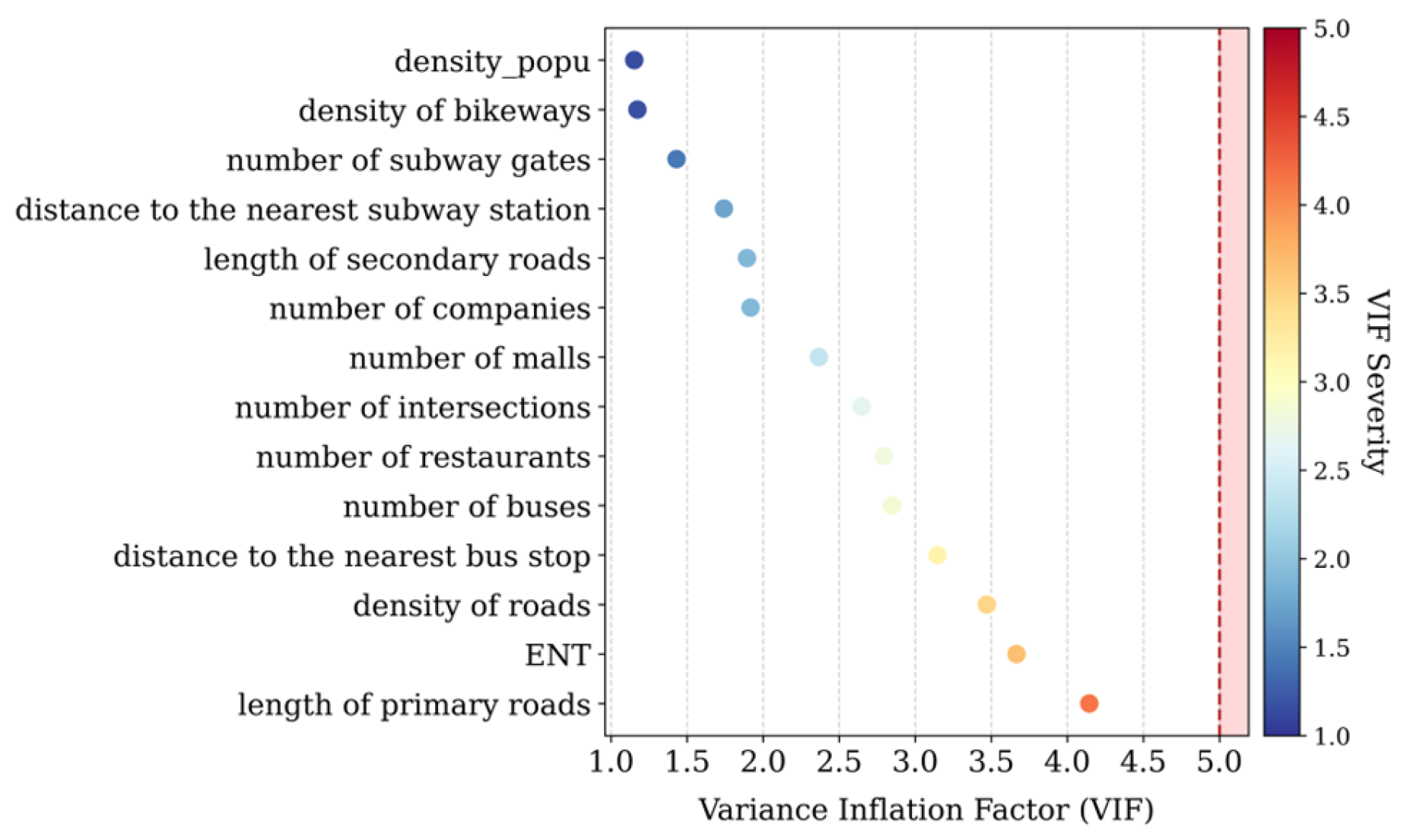
- Salmerón, R.; García, C.B.; García, J. Variance inflation factor and condition number in multiple linear regression. J. Stat. Comput. Simul. 2018, 88, 2365–2384. [Google Scholar] [CrossRef]
- Song, Y.; Merlin, L.; Rodriguez, D. Comparing measures of urban land use mix. Comput. Environ. Urban Syst. 2013, 42, 1–13. [Google Scholar] [CrossRef]
- Aydin, Z.E.; Erdem, B.I.; Cicek, Z.I.E. Prediction bike-sharing demand with gradient boosting methods. Pamukkale Univ. J. Eng. Sci. 2023, 29, 824–832. [Google Scholar] [CrossRef]
- Chen, T.Q.; Guestrin, C. XGBOOST: A scalable tree boosting system. In Proceedings of the 22nd ACM SIGKDD International Conference on Knowledge Discovery and Data Mining, San Francisco, CA, USA, 13–17 August 2016. [Google Scholar] [CrossRef]
- Simon, R.; Elena, M.; Omar, A.K. Predictive modeling for optimization of field operations in bike-sharing systems. In Proceedings of the 2019 6th Swiss Conference on Data Science (SDS), Bern, Switzerland, 14–15 June 2019. [Google Scholar] [CrossRef]
- Wang, X.X.; Zheng, S.Q.; Wang, L.Q.; Han, S.; Liu, L. Multi-objective optimal scheduling model for shared bikes based on spatiotemporal big data. J. Clean. Prod. 2023, 421, 138362. [Google Scholar] [CrossRef]
- Miranda-Moreno, L.F.; Lahti, A.C. Temporal trends and the effect of weather on pedestrian volumes: A case study of Montreal, Canada. Transport. Res. Part D Transport. Environ. 2013, 22, 54–59. [Google Scholar] [CrossRef]
- Hsu, C.K.; Rodríguez, D.A. A comparison of heat effects on road injury frequency between active travelers and motorized transportation users in six tropical and subtropical cities in Taiwan. Soc. Sci. Med. 2024, 360, 117333. [Google Scholar] [CrossRef] [PubMed]
- Márquez, L.; Cantillo, V.; Arellana, J. How do the characteristics of bike lanes influence safety perception and the intention to use cycling as a feeder mode to BRT? Travel Behav. Soc. 2021, 24, 205–217. [Google Scholar] [CrossRef]


| Start Time | End Time | Start Latitude | Start Longitude | End Latitude | End Longitude |
|---|---|---|---|---|---|
| 2021-05-10 16:37:36.0 | 2021-05-10 16:45:12.0 | 22.596647 | 114.138533 | 22.603652 | 114.139904 |
| Dimension | Variable Names | Mean | Variance |
|---|---|---|---|
| Density | density of bikeways | 5.65 | 14.28 |
| density of roads | 125.92 | 103.45 | |
| Diversity | ENT | 0.74 | 0.29 |
| number of companies | 18.76 | 36.68 | |
| number of interests | 0.88 | 1.05 | |
| number of malls | 34.68 | 90.16 | |
| Design | number of intersections | 1.39 | 2.00 |
| number of buses | 1.39 | 2.00 | |
| number of subway gates | 0.55 | 1.82 | |
| Destination Accessibility | length of the primary roads | 990.08 | 1351.39 |
| length of the secondary roads | 503.56 | 743.09 | |
| Distance to Transit | distance to the nearest bus stop | 0.54 | 0.50 |
| distance to the nearest subway station | 1.46 | 1.18 |
| Models | R2 | MAE | RMSE2 |
|---|---|---|---|
| RF | 0.804 | 6.542 | 10.572 |
| LightGBM | 0.759 | 9.267 | 15.631 |
| XGBoost | 0.723 | 11.438 | 19.685 |
| MLP | 0.726 | 10.741 | 17.529 |
| CNN | 0.712 | 10.298 | 18.023 |
Disclaimer/Publisher’s Note: The statements, opinions and data contained in all publications are solely those of the individual author(s) and contributor(s) and not of MDPI and/or the editor(s). MDPI and/or the editor(s) disclaim responsibility for any injury to people or property resulting from any ideas, methods, instructions or products referred to in the content. |
© 2025 by the authors. Licensee MDPI, Basel, Switzerland. This article is an open access article distributed under the terms and conditions of the Creative Commons Attribution (CC BY) license (https://creativecommons.org/licenses/by/4.0/).
Share and Cite
Shen, Y.; Zhang, L.; Song, Y.; Wang, C.; Yu, Z. Nonlinear Influence of Urban Environment on Dockless Shared Bicycle Travel Patterns. Sustainability 2025, 17, 4575. https://doi.org/10.3390/su17104575
Shen Y, Zhang L, Song Y, Wang C, Yu Z. Nonlinear Influence of Urban Environment on Dockless Shared Bicycle Travel Patterns. Sustainability. 2025; 17(10):4575. https://doi.org/10.3390/su17104575
Chicago/Turabian StyleShen, Yonggang, Long Zhang, Yancun Song, Chengquan Wang, and Zhenwei Yu. 2025. "Nonlinear Influence of Urban Environment on Dockless Shared Bicycle Travel Patterns" Sustainability 17, no. 10: 4575. https://doi.org/10.3390/su17104575
APA StyleShen, Y., Zhang, L., Song, Y., Wang, C., & Yu, Z. (2025). Nonlinear Influence of Urban Environment on Dockless Shared Bicycle Travel Patterns. Sustainability, 17(10), 4575. https://doi.org/10.3390/su17104575