Abstract
Currently, regional flood research often lacks a synergistic assessment of both flood occurrence risk and flood duration, limiting the comprehensive understanding needed for sustainable disaster risk reduction. To address this gap, this study applies advanced machine learning approaches to assess flood hazards in the Yangtze River Delta, one of China’s most economically and environmentally significant regions. Specifically, XGBoost is employed to evaluate flood occurrence risk, while LSTM is used to predict flood duration. A novel flood risk index (FRI) is proposed to quantify the integrated risk by combining these two dimensions, supporting more sustainable and effective flood risk management strategies. Furthermore, SHAP analysis is conducted to identify the most critical factors contributing to flooding. The results demonstrate that XGBoost delivers strong predictive performance, with average precision, recall, F1-score, accuracy, and AUC values of 0.823398, 0.831667, 0.827090, 0.826435, and 0.871062, respectively. Areas with high flood risk, long duration, and elevated FRI values are mainly concentrated in major river basins and coastal zones. The range of flood risk spans from 0.000073 to 0.998483 (mean: 0.237031), flood duration from 0.223598 to 2.077040 (mean: 0.940050), and FRI from 0 to 0.934256 (mean: 0.091711). Cities with over 40% of their areas falling in medium to high FRI zones include Suzhou (48.99%), Jiaxing (48.07%), Yangzhou (46.87%), Suqian (44.19%), Changzhou (43.43%), Wuxi (43.20%), Lianyungang (42.21%), Yancheng (40.88%), Huai’an (40.73%), and Bengbu (40.06%). SHAP analysis reveals that elevation and rainfall are the most critical factors influencing flood occurrence, underscoring the importance of integrating environmental variables into sustainable flood risk governance.
1. Introduction
Floods are among the most frequent and devastating natural disasters. Each year, they cause significant loss of life and economic damage [1,2]. With global climate change, increasing extreme weather events, and rapid urbanization, large-scale and long-duration floods are expected to become more frequent in the future. Therefore, assessing flood risk is essential for effective flood control and sustainable development.
Modeling plays a key role in studies of flood risk assessment. Kumar reviewed and organized several common flood analysis models [3], including hydrologic and hydraulic modeling, numerical flood modeling, rainfall–runoff modeling, remote sensing and GIS-based flood modeling [4], multiple-criteria decision analysis-based flood management (MCDA) [5,6], and models based on artificial intelligence (AI) and machine learning (ML). However, hydrodynamic and rainfall–runoff models are more suitable for localized sub-watershed studies [7]. Comparatively, GIS-based and machine learning approaches are preferred.
With advances in computing and algorithms, machine learning has emerged as an efficient and accurate tool for flood prediction. Algorithms such as random forest (RF), support vector machine (SVM), and extreme gradient boosting (XGBoost) have been widely applied [8]. For example, RF was used to predict flood risk in the Dongjiang River Basin, China, and was shown to be highly reliable [9]. SVM has been employed to evaluate flood sensitivity in the Kuala Lumpur Basin, Malaysia, proving to be an effective tool [10]. Additionally, the frequency ratio (FR) method was combined with SVM using a radial basis function kernel to assess flood probability in Malaysia [11]. In addition to supervised learning, semi-supervised methods like the weakly labeled support vector machine (WELLSVM) have shown promising results in flood response studies in Beijing [12].
Traditional models such as RF, SVM, and multi-layer perceptron (MLP) are well-established in flood assessment. Newer methods like gradient-boosted decision trees (GBDT), XGBoost, and one-dimensional convolutional neural networks (1D-CNN) have seen relatively limited application [13]. In one study, XGBoost, combined with particle swarm optimization (PSO), was used to assess flood frequency at the national scale in Iran. It outperformed RF and support vector regression (SVR) across all flood quartiles [14].
The Yangtze River Delta (YRD) has become a key region of interest for flood studies. Zhu et al. used machine learning methods such as XGBoost to assess flood susceptibility in the YRD urban agglomeration [15]. A study proposed a framework for assessing urban flood resilience based on the PSR-SENCE model, which assessed the flood resilience of 27 cities in the YRD [16]. Deng et al. identified population density, land use, and precipitation intensity as key factors influencing heavy rainfall disasters in the region [17]. Zhang et al. analyzed how population exposure changes under multiple storm scenarios, finding significant spatial and temporal variation in the YRD [18]. These studies highlight the region’s vulnerability and the need for sustainable flood risk management.
However, most existing research focuses only on pre-flood risk. The hazards caused by long-duration floods and extensive inundation areas are often overlooked [19]. This indicates a gap in current disaster risk frameworks. Many fail to consider the temporal dimension of floods, which is crucial for a comprehensive understanding of disaster impacts. This perspective aligns with the principles of the Sendai Framework for Disaster Risk Reduction, which calls for more holistic and sustainable approaches to disaster management.
We apply two machine learning methods, XGBoost and LSTM, to predict and analyze flood risk in the YRD. This study fills a gap in previous research that focused only on either flood risk or flood duration. We propose a coupled prediction approach that considers both aspects. The flood risk index (FRI) is introduced to quantify the integrated hazard level. By combining spatial and temporal dimensions, this method aligns with multi-dimensional disaster risk frameworks. It also supports sustainable flood management under climate change and urbanization. The study addresses two scientific questions: (1) What is the geographical distribution of potential flood risk areas and flood duration in the YRD? (2) What are the most critical factors contributing to flooding in this region? The remainder of this paper is organized as follows: Section 2 presents the study area and methodology; Section 3 discusses the pre-flood risk, post-flood inundation levels, FRI and SHAP results; Section 4 analyzes the causes and measures of the risks and hazards, resolution, flood management references and limitations; Section 5 concludes the study. The framework of the study is shown in Figure 1.
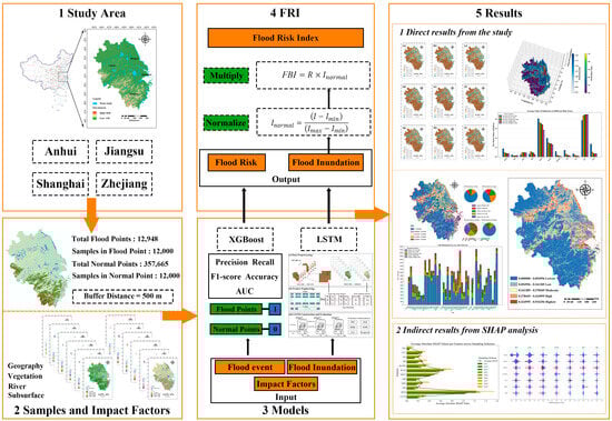
Figure 1.
This is the framework of this study. This study can be divided into five segments. Firstly, the research scope of this study is defined as three provinces and one city in the YRD. Secondly, based on the flood map, the sample area is tested, and the distribution of flood impact indicators is provided. Thirdly, a machine learning process is performed based on the comparison of the model assessment as a way to obtain the predicted flood risk and duration, so that the FRI can be extracted as a measure of the combined flood risk. Finally, visualization maps and SHAP analysis maps are obtained, respectively.
2. Materials and Methods
2.1. Materials
2.1.1. Study Area
The YRD is located in eastern China and includes parts of the provinces of Shanghai, Jiangsu, Zhejiang, and Anhui. Considering the completeness of the provincial administrative divisions, the study area of this paper includes the complete divisions of three provinces and one city. Geographically, the entire study area encompasses the core area of the YRD, with latitudes ranging from 27.2° N to 35.1° N, and longitudes ranging from 114.9° E to 123.1° E (Figure 2), covering a watershed area of about 27,250 square kilometers. According to CLCD land use data, the YRD features a dense network of rivers and lakes, with a water surface ratio of 7.36%. The region experiences a subtropical monsoon climate characterized by high temperatures and abundant rainfall during the same season, along with distinct seasonal variations. The landscape primarily consists of the East China Plains and the hilly areas of southern Zhejiang and Anhui, with a gently undulating topography and a general decline in elevation from west to east.
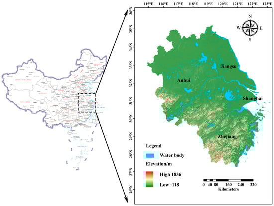
Figure 2.
This illustration shows the research region and the attribution of elevation and waterbodies. The picture is from https://www.tianditu.gov.cn/ (accessed on 15 October 2024).
The YRD is the most frequently flooded and threatened region in China. Influenced by the monsoon climate, typhoons, low topography, and a dense river network, flooding events occur frequently and show a trend of increasing intensity and scope. With the rollout of the YRD Integrated Development Plan, the region has entered a new stage of coordinated growth. During the 14th Five-Year Plan, ecological security became a national priority, making disaster prevention and mitigation a key focus in the YRD. Therefore, setting the study area as the YRD exhibits both practical urgency and scientific support for regional governance and flood control policies.
The base map of the China region was sourced from the Standard Map Service System of the National Geographic Information Public Service Platform, at a scale of 1:20 million. It depicts the officially recognized boundaries of China, without including neighboring countries or modifying the original content of the map.
2.1.2. Sample
In flood hazard studies, historical flood events are crucial data sources. In this study, the Global Flood Database v1 (2000–2018) [20] from the Google Earth Engine platform was selected and extracted for the study area. This dataset includes maps depicting the extent and temporal distribution of 913 flood events between 2000 and 2018. In this study, the Sentinel-1 SAR dataset (COPERNICUS/S1_GRD) provided by the Google Earth Engine platform was used in order to obtain flood data from 2019 to 2024, and the flood event points were extracted with reference to the methodology suggested in Ref. [21]. The resolution was standardized to 1000 m × 1000 m during geoprocessing, with the pixel values in flood zones assigned a value of 1, and those in non-flood zones assigned a value of 0.
This was achieved using the Create Random Points tool in ArcMap, which generates random sample points within a vector map of points derived from the flood map. To balance the number of sampling points in both flood and non-flood areas, a total of 24,000 sample points were selected, with 12,000 points in the flood zone and 12,000 points in the non-flood zone. A buffer distance of 500 m was used. In ArcMap, a buffer width of 500 m is used during random sampling. This ensures that each sampling area fully covers a 1000 m × 1000 m raster cell, without overlapping multiple cells, thus reducing spatial confusion. A buffer smaller than 500 m may cause sample points to cluster too closely, reducing spatial representatives. In contrast, a buffer larger than 500 m may space the points too far apart. This increases the risk of missing some flood points, especially those located within the buffer zones of neighboring samples. Sampling was conducted in three batches, and each batch was repeated three times, as shown in Table 1. The final sampling plan consists of nine sampling programs, labeled from A11 to A33, created by combining different parts of the same batch.

Table 1.
Specific programmers for random point sampling.
2.1.3. Impact Factors for Flood Assessment
In order to accurately predict and assess floods, the selected indicator system should be reasonable and highly relevant to flood occurrence. In this study, 12 indicators were selected to assess the risk of flooding and the duration of inundation, covering four dimensions: geographic, vegetation, fluvial, and subsurface. This study focuses on predicting the probability of flooding, especially using machine learning models, and thus prioritizes physical geographic and meteorological hydrological factors that are directly related to flooding, such as rainfall, topography, and soil properties. This assessment system is reasonable in the field of flood risk assessment, in contrast to a study in Quang Binh Province, Vietnam, which mainly considered physical factors such as topography, slope, and rainfall, without incorporating socioeconomic variables [22]. In addition, Liu et al. proposed the flood genome model, which focuses on physical factors such as topography, hydrology, and built environment, while socioeconomic variables were not included in the model [23]. Thus, in this study, there are considerations of socioeconomic factors, which will be discussed in depth in Section 4.
The geographic dimension includes eight elements (Table 2): elevation (based on the digital elevation model, DEM), slope (SLOPE), average annual rainfall (RAIN), China land cover data (CLCD), the stream power index (SPI), the sediment transport index (STI), the topographic wetness index (TWI), and the topographic control index (TCL). The vegetation dimension is represented by the normalized difference vegetation index (NDVI), while the river dimension includes the distance to the river (DIS). The subsurface dimension comprises the density of pipeline networks (DPN) and the impervious surface ratio (ISR).
Table 2.
Detailed information for each indicator.
2.2. Methods
2.2.1. Model Selection
Previous studies have shown that GBDT, XGBoost, and RF generally achieve higher accuracy in predicting flood risk compared to that of other machine learning models [13]. However, due to differences in study areas and sample characteristics, it is not appropriate to select a single model without conducting a comparative analysis.
XGBoost is an efficient implementation of the GBDT algorithm. It improves model performance by combining the outputs of multiple decision trees. This method was first introduced by Chen and Guestrin [26]. The main process within a cycle of XGBoost consists of solving for the initial predictions (initializing the model), adding iterations and training each tree, calculating the residuals, and fitting a new tree, thus updating the predictions (1)–(3):
where is the initial projected value, and the target values of all samples are averaged and used as the initial predicted value; is the iterative updating component, which represents updating the final prediction by accumulating the predicted values of the fitted new tree in each round of iteration; is the first-order derivative (gradient) of the loss function, which is used to reflect the error in the current prediction; is the second-order derivative of the loss function (Hessian), which is used to regulate the update step; is the ratio of learning, used to control the influence of each tree in order to progressively approximate the optimal solution.
Random forest is an integrated learning model based on the idea of bagging (self-help method). Multiple decision trees are constructed by randomly sampling the training data, and each tree is trained on a randomly selected subset of features. The final prediction is determined by voting (classification task) or averaging (regression task) across all trees [9].
Gradient boosting decision tree (GBDT) is an effective machine learning algorithm based on an integrated approach to decision trees. It improves the performance of a model by progressively training a series of weak learners (usually decision trees), optimizing each prediction based on the residuals of previous models, and the function can be expressed as follows (4):
where is the final result of the prediction; is the initial projected value; is the ratio of learning; is the decision tree model constructed in the iteration, which serves to fit the residuals of the previous model.
In order to identify the top-performing model in this study, five performance metrics, i.e., precision, recall, F1-score, accuracy, and AUC, were selected to compare the strengths and weaknesses of the three models. Precision represents the proportion of samples predicted as positive by the model that are actually positive, reflecting the accuracy of the positive predictions. Recall measures the proportion of actual positive samples that are correctly predicted as positive, indicating the model’s ability to cover positive cases. F1-score, which is the harmonic mean of precision and recall, helps balance the two metrics, especially for imbalanced datasets. Accuracy shows the proportion of correctly predicted samples out of the total, but it can be misleading for datasets with unbalanced categories. AUC (area under the ROC curve) assesses the overall performance of the model across different classification thresholds, with the ROC curve plotting the false-positive rate on the horizontal axis and recall on the vertical axis. AUC values closer to 1 indicate better model performance in distinguishing between positive and negative classes.
When flood duration needs to be predicted, the binary machine learning used for risk prediction is no longer applicable. Instead, flood duration often needs to be predicted with the help of a time series forecasting model, so finding and identifying a model that performs well is necessary.
Performance comparisons between models are usually made in LSTM, CNN, ANN, SVM, and MLP [27]. Numerous research results have shown that LSTM performs well when dealing with either short or long-time sequences [28,29,30,31]. Considering this, LSTM is used as a flood inundation time prediction model in this study.
The LSTM model is affiliated with recurrent neural networks (RNN), and the main nodes include forgetting gates (5), input gates (6) and (7), memory units (8), and output gates (9) and (10). At each time step, the workflow consists of forgetting, information updating, memory unit updating, and outputting [32]. The main functions are shown, as follows:
where is the forgetting gate, which determines how much past information is forgotten; is the input gate, which decides the importance of the present information; is candidate memories; represents the process of updating the memory cells; is the output gate that determines the next moment’s hidden layer state; is the sigmoid activation function; tanh is hyperbolic tangent activation function; is the weight matrix of the forgetting gate; and are, respectively, the weight matrix of the input gates and the candidate memories; is the weight matrix of the output gate; is the hidden layer state at the previous moment; is the input at the current moment; and are the corresponding bias terms.
In this study, Python, version 3.11.10; pandas, version 2.2.2; XGBoost, version 2.1.1; PyTorch, version 2.2.2; and matplotlib, version is 3.9.2, are used. The scikit-learn version information is as follows: uname_result (system = Windows 10, node = DESKTOP-9VMC0KN, release = 10, version = 10.0.19045, machine = AMD64). The operating system is Windows 10; the CPU is Intel64 Family 6 Model 158 Stepping 9, Genuine Intel. Total training time for flood risk is about 10 min, and total time for flood inundation is about 3 h 34 min.
2.2.2. Flood Risk Index
Duration is an important indicator of the hazardousness of a disaster, but it is unscientific to simply predict duration while ignoring the preconditions for the occurrence of a disaster. In order to obtain an assessment index that takes both into account, this study multiplies the risk (probability) of flood occurrence and the normalized duration of flooding to obtain a composite hazard index of flooding. The theoretical basis for this is that the composite risk in areas at low risk of flooding is also generally low, regardless of the estimated duration, and that an anomaly in one of these values does not lead to an anomaly in the composite risk. Similar ideas can be found in the studies of Qi, Apel et al. in regards to calculating the composite risk score [33,34].
is calculated by the following formula:
where is the composite hazard index of flooding; is the risk of flooding, which will be predicted by XGBoost; is the inundation of flooding, which will be predicted by LSTM; is standardized by min–max normalization. For example, if the predicted flood duration at a pixel point is 5 days ( = 5), the minimum value of flood duration in all samples is 2 days ( = 2), and the maximum value is 10 days (), then the standardized flood duration for that pixel is 0.375 ().
2.2.3. Shapley Additive Explanations (SHAP)
SHAP (Shapley additive explanations) is an ex post model interpretation method that calculates the marginal contribution of features to the model’s output, allowing for interpretation of black-box models at both global and local levels. This method effectively overcomes the abstract input–output relationship in machine learning, providing a reasonable quantification of the contribution of each feature. Given that SHAP can be applied to XGBoost, this study uses it to assess the interpretability of flood risk predictions.
Firstly, the SHAP values for each feature will be calculated, and bar charts will be plotted to visualize these contributions. The SHAP model computes a contribution value for each feature, indicating how the feature’s value influences the final prediction. This contribution can be positive (increasing the predicted value) or negative (decreasing the predicted value). By plotting the contribution histograms, we can identify which features are most influential in the model’s predictions and understand their impact on the predicted outcomes.
Secondly, based on the aggregated SHAP values of all indicators, summary plots will be generated. These plots serve as a visualization tool to present the importance of each feature and its relationship with the predicted outcomes.
3. Results
3.1. Index Distribution in Research Region
The source data for each indicator were processed using ArcMap to obtain their distribution across the YRD region, with all indicators standardized to a spatial resolution of 1000 m × 1000 m. The values of the twelve indicators were then assigned to the sampling points from each of the previously generated sampling programs using the Value Extraction to Points tool. This process outputs a table containing sampling point information with twelve indicator columns and one flood event column, which will serve as part of the input data for training the XGBoost model.
Figure 3 illustrates the spatial distribution characteristics of the key geo-environmental factors involved in the flood risk analysis of the Yangtze River Delta region: (a) indicates the land use types in the study area, whose spatial distribution affects the surface runoff path and infiltration capacity, and is an important basis for the identification of flood-prone areas; (b) shows the topographic relief extracted based on the digital elevation model (DEM), which is used for the identification of low-lying and waterlogging-prone areas; (c) is the Euclidean distance to the river, which reflects the proximity of each parcel to the source of flooding and is a key factor in assessing flood exposure; (d) is the density of built-up areas, which is calculated from official land-use data and is used to measure the degree of urbanization, thus reflecting the load on the drainage system and the responsiveness to heavy rainfall; (e) indicates the proportion of impermeable surfaces, such as dense areas of roads and buildings, which can significantly reduce surface water; (e) is the proportion of impermeable surfaces, such as roads and built-up areas, which significantly reduces the permeability of surface water and increases the risk of urban flooding; (f) is the normalized vegetation index (NDVI), which reflects the degree of surface vegetation cover, and is closely related to the soil retention and water regulation capacity; (g) represents the spatial pattern of the average annual precipitation in the past two decades, which helps to identify the areas of perennial heavy precipitation; (h) is the distribution of slopes, which influences the speed and convergence path of the surface water flow and is an important parameter for the characterization of the terrain control capacity; (i) is the runoff power index (SPI), which can be used to reflect the erosive capacity and energy distribution of flood water flow; (j) is the sediment transport index (STI), which estimates the sediment transport capacity of surface water flow and affects the degree of downstream siltation and drainage smoothness; (k) is the terrain moisture index (TWI), which reveals the possibility of terrain waterlogging and is used for the identification of potential wet flooded areas; (l) is the terrain control index (TCL), which combines multiple topographic factors to reflect the role of geomorphological structure in regulating flood aggregation and dispersion. Through the spatial visualization of these factors, flood-prone areas can be comprehensively identified, and geographic support can be provided for refined risk assessment and disaster prevention decision making.
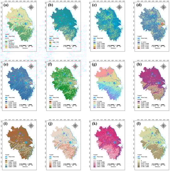
Figure 3.
(a) Describes the land use type within the study area; (b) represents the elevation within the study area using a numerical elevation model; (c) is the distance from the river, expressed through the Euclidean distance; (d) is the density of the official website in the built-up area; (e) represents the rate of impermeable surfaces; (f) is the NDVI (normalized difference vegetation index); (g) represents the twenty-year average annual rainfall in the study area; (h) is the gradient; (i) represents the stream power index; (j) denotes the sediment transport index; (k) is the topographic wetness index; (l) is the topographic control index.
3.2. Flood Risk Forecast
This study applies the GridSearchCV method to perform a combinatorial search of multiple hyperparameters. It exhaustively explores all possible combinations within the specified parameter space and selects the set that performs best during cross-validation. To balance the model’s learning ability and generalization capacity, the selected parameters, as listed in Table 3, contribute jointly to model structure, training speed, and resistance to overfitting. The search space includes a total of 3 × 3 × 2 × 2 × 2 = 72 parameter combinations. For each combination, tri-fold cross-validation is conducted on the training set. The training data are divided into three equal parts, with two used for training and one for validation. This process is repeated three times, and the average accuracy is calculated to evaluate model performance. This ensures that the evaluation results are stable and representative. To guarantee the reproducibility and comparability of the results, a fixed random seed (random seed = 42) is set throughout the training data split, sampling, and model initialization steps. This eliminates the uncertainties caused by random variation.
Table 3.
Parameter network values for GBDT, XGBoost, and RF.
This study divides the data from 2000–2018 as the model training set and introduces the random sampling scheme below. The data from 2019–2024 are used as the model test set and validation set. The overall sample size ratio of the training set, test set, and validation set are controlled as 6:2:2 to evaluate the performance of the GBDT, XGBoost, and RF models. The results in Table 4 show that the mean values of five statistical indexes for both GBDT and XGBoost are higher than 0.8, indicating excellent model performance: XGBoost > GBDT > RF.
Table 4.
Model performance evaluation results.
Compared with GBDT, XGBoost is an optimized version with several advantages. It offers higher computational efficiency and built-in regularization. It also automatically handles missing values and provides stronger explanations of feature importance. The superiority of XGBoost has been demonstrated in data-driven flood alert systems [35]. Therefore, XGBoost is selected as the predictive model for flood risk in this study.
Due to the random nature of the sampling scheme creation, there is some variation in the predictions produced by different schemes. To identify the sampling scheme that best fits the model and yields the best prediction results, this study calculates the true positive and false positive rates for each sampling scheme and plots the ROC curves to determine the optimal threshold with the AUC for each scheme. The optimal threshold is defined as the cutoff point that maximizes the kappa coefficient, which is used to delineate the 0–1 labeling.
As shown in Table 5, among all sampling scenarios, the metric values are above 0.8, suggesting good model performance. However, A11, A12, and A13 show recall values below 0.8, indicating lower sensitivity in detecting flood-prone areas. Among all schemes, A32 achieves the highest kappa coefficient (0.702853) at the optimal threshold, reflecting stronger agreement with actual flood occurrences. It also shows a well-balanced performance in regards to precision (0.843686), recall (0.854583), and F1-score (0.849100). Additionally, A32 shows higher accuracy (0.848125) and AUC (0.870202) scores. Based on these results, A32 is chosen as the baseline sampling scheme for flood risk prediction due to its strong reliability and classification capability. The ROC curve of the model under nine sampling schemes is shown in Figure 4. The confusion matrix shows TN (true negative) in the upper left, FP (false positive) in the upper right, FN (false negative) in the lower left, and TP (true positive) in the lower right.
Table 5.
Comparison among sampling schemes.
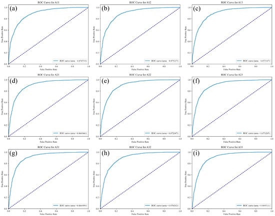
Figure 4.
The ROC curves for sampling programmers A11 to A33 correspond to (a–i), respectively. These are used to evaluate the model’s classification performance under different thresholds. The ROC curve plots the false positive rate (FPR) on the horizontal axis and the true positive rate (i.e., recall) on the vertical axis. The curve shows a trend of rapid increase, followed by gradual flattening. This indicates that the model achieves a high recall rate even at low false positive rates, suggesting strong recognition ability. The dashed line represents the baseline of random classification. The model’s curve lies well above this line, showing much better discriminative power than that of random guessing. The area under the ROC curve (AUC) reflects the model’s overall classification performance. A value closer to 1 indicates stronger accuracy across different thresholds. This figure provides a visual reference for comparing the performance of different sampling schemes.
The trained XGBoost model was then used to reprocess all the image point metrics in the YRD region to obtain the expected risk values (ranging from 0 to 1) for each image point. The entire region was classified into five risk zones—highest risk, high risk, moderate risk, low risk, and lowest risk—using the natural intermittent points classification (Jenks) method.
As showed in Figure 5h, the flood risk ranges from 0.000073 to 0.998483, with a mean value of 0.237031. The high-value areas are mainly concentrated in large river basins and coastal regions, including the Huaihe River Basin, Yangtze River Basin, Taihu Lake Basin, Qiantang River Basin, and the coastal areas of the East China Sea. Clearly, flooding in the YRD region is primarily caused by the inundation of rivers, lakes, and seas.
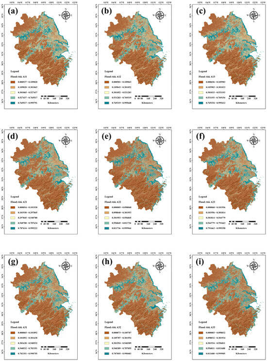
Figure 5.
(a–i) represent scenarios A11–A33, respectively.
From a provincial perspective, Shanghai has the largest proportion of high-risk areas, accounting for 40.86%, largely due to its coastal lowlands and extensive mudflat areas. Following Shanghai, Jiangsu has 19.98% of its area classified as high-risk, mainly due to its long coastline and vast watershed. Zhejiang Province ranks next, with 9.63% of the high-risk areas, a result of its hilly terrain covering a larger part of the province. Finally, Anhui Province has the smallest proportion of high-risk areas at 8.66%, primarily due to its distance from the coast, higher elevation, and more mountainous terrain.
The mean values of the indicators and the proportion of high-risk areas within each province are summarized in Figure 6. The indicators vary significantly across different flood risk levels. NDVI and DEM values decrease as the flood risk increases, indicating that areas with lower vegetation cover and elevation are more prone to flooding. RAIN, SLOPE, SPI, STI, and TWI are also lower in high-risk areas, suggesting that gentle topography, poor drainage, and high rainfall contribute to waterlogging. DPN and ISR are slightly higher in high-risk areas, indicating that urbanization affects water flow paths and flood risk. TCL remains high across all risk levels, showing the overall influence of topography on water flow. This analysis highlights the environmental characteristics of high-risk flood areas, aiding in risk identification.
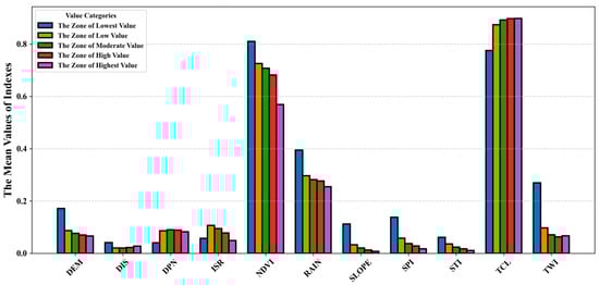
Figure 6.
This is the distribution of indicators in different zones, which shows the normalized mean values of the indicators in areas with different flood risk classes. The horizontal coordinates are the indicator names, the vertical coordinates are the indicator means, and the bar colors represent the different risk class areas.
3.3. Flood Inundation Forecast
The workflow of LSTM can be divided into three stages: data preprocessing, feature engineering, LSTM construction and evaluation; the workflow of the LSTM employed in this study is illustrated in Figure 7.
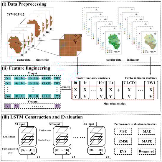
Figure 7.
The framework of LSTM, which consists of three main nodes, in order of data preprocessing, feature engineering, and LSTM construction and evaluation. In section (i), the sources and proportions of the training, test, and validation sets are consistent with the process of flood risk forecast. Two sets of data will be read as the data source for the LSTM, including 12 sheets of raster data storing the evolution of the flood and tabular data containing features and coordinates of image points. Each iteration reads 12 raster files (each corresponding to a different point in time) and combines them into a 3D array of shape (t, H, W), with t denoting the number of time steps, H and W being the height and width of the raster, and the array value being (12, 1,1). The purpose of outputting this array is to provide a structure that facilitates the subsequent extraction of the time series of specific image elements by time step. In section (ii), traversing the whole raster image by image, the time series of each image point at all time steps are extracted through the time dimension and combined with the corresponding metrics to form a feature vector X. At the same time, the corresponding target variable (flood duration) is stored in y. In section (iii), a three-layer LSTM model is defined using PyTorch to learn the relationship between the time series data and flood duration. The input layer receives the time series features and indicators, while the hidden layers capture the dynamics of the time series through multiple LSTM cells. The prediction results are then output through a fully connected layer.
All in all, a three-layer LSTM model is constructed based on PyTorch for predicting flood duration by combining time series data for the flood evolution process and related indicators. The model uses a fixed time window length of 12, corresponding to 12 different moments of raster data. The input data is initially structured as a 3D array with the shape (t, H, W), which is subsequently converted into a pixel-by-pixel time series and combined with static features to form an input tensor with the shape [N, 12, F], where N is the number of samples, and F is the number of features. The model contains three layers of LSTM with 100 hidden units per layer and uses a dropout rate of 0.5 to prevent overfitting; the final prediction results are output through a fully connected layer. The model is trained using the ADAM optimizer, with the learning rate set to 0.001, and the loss function is the mean square error (MSE). The batch size is 32, the number of training rounds is 500, and all hyper-parameters are determined by grid search, as listed in Table 6. The division ratio of the training set, validation set, and test set is consistent with the flood-risk prediction stage.
Table 6.
The search space and the optimized hyperparameters.
It has been shown that batch size can influence the accuracy of model predictions. This study records the changes in the MSE loss function for each batch size, as shown in Figure 8. During the training process of the LSTM model, the loss values show an overall decreasing trend, indicating that the model is continuously optimized and gradually reduces the prediction error. The trends of training loss, validation loss, and testing loss are generally consistent, indicating that the model can fit the training data effectively and that it exhibits good generalization ability. Although there are small fluctuations in some epochs, such fluctuations are reasonable and are usually due to the diversity of data batches, as well as to natural fluctuations when the model is fine-tuned around local optimal solutions. Overall, neither the smooth decline in loss nor the small fluctuations affect the stability of the model and the final fit. In terms of the evaluation metrics, the model performs well, especially with high R-squared scores and variance explained, indicating better prediction. When the batch size is 32, the loss values show an overall decreasing trend. Training loss drops from 0.738 to 0.065, validation loss from 1.023 to 0.082, and testing loss from 0.873 to 0.085. The small loss gap (0.0168) indicates consistent fitting between training and validation sets, without significant overfitting. The high R2 score of 0.9172 reflects strong predictive power, and the smoothing degree of 0.0215 shows stable training. Although there are some fluctuations, this is typical of the LSTM model’s optimization process.
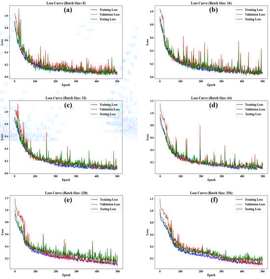
Figure 8.
The loss curve for each batch size. Each figure corresponds to a different batch size, (a) corresponds to a batch size of 8; (b) of 16; (c) of 32; (d) of 64; (e) of 128; (f) of 256.
On one hand, batch size is used to verify whether the parameter results align with expectations after the grid search; on the other hand, it helps assess whether the model’s convergence of the loss function is reasonable under the current parameters. The results of the model performance evaluation are presented in Table 7.
Table 7.
Results of the model performance evaluation.
The results show that the optimal batch size of this model is 32, which is consistent with the hyperparameter tuning results, and the model performs more satisfactorily in this case.
The geographical distribution of flood duration is presented in Figure 9 using a three-dimensional bar chart. Duration represents the average flood duration over a future sampling period of 25 years. The results show that the duration ranges from 0.223598 to 2.077040, and the mean value is 0.940050, with areas of higher flood duration (above the mean value) predominantly concentrated in the Yangtze River, Huaihe River, and Taihu Lake basins, as well as along the coasts of Hangzhou Bay and the East China Sea.
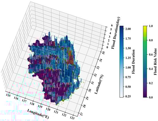
Figure 9.
The 3D geographical distribution of flood duration.
3.4. FRI
In this study, the results derived in Section 3.2 and Section 3.3 were calculated using the methodology outlined in Section 2.2.2 to obtain the geographic distribution of the composite flood hazard. FRI ranges from 0 to 0.934256 with a mean value of 0.091711. The distribution was then categorized into five levels—low, lower, moderate, higher, and high—using the natural intermittent points classification (Jenks) method, and the lowest-low, low-moderate, moderate-high, and high-highest thresholds were 0.054956, 0.161205, 0.278445, and 0.424995, respectively.
We divided the ranked districts into provincial administrative regions and plotted the percentage of districts in each rank within each province, as shown in Figure 10. The results indicate that the proportion of moderate and high-risk areas in Shanghai and Jiangsu provinces reached 52.2% and 36.3%, respectively, while the proportions in Anhui and Zhejiang provinces were relatively smaller, at 16.9% and 16.5%, respectively.
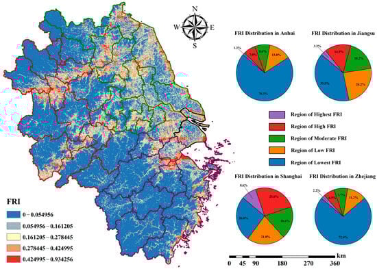
Figure 10.
Provincial distribution of FRI values.
To further explore the distribution of different FRI classes in the municipalities, this study divides the data by municipal area and presents stacked maps of the FRI class areas for each city, as shown in Figure 11. The y-axis represents the number of image points, which is equivalent to the area of each class. Line graphs were plotted for low and moderate regions to indicate the municipal weight of moderate and high-risk areas. Zhoushan and Huainan display medium and high-risk zones exceeding 50%, with values of 57.34%, 52.94%, and 52.21%, respectively. Ten cities—Suzhou, Jiaxing, Yangzhou, Suqian, Changzhou, Wuxi, Lianyungang, Yancheng, Huai’an, and Bengbu—have medium-high value zones exceeding 40%, with values of 48.99%, 48.07%, 46.87%, 44.19%, 43.43%, 43.20%, 42.21%, 40.88%, 40.73%, and 40.06%, respectively. These cities are typically located in coastal regions or large river basins and are characterized by low-lying areas. Cities with more than 30% but less than 40% of medium-high value zones include Nantong, Taizhou, Ningbo, Wuhu, Tongling, and Maanshan. Cities with less than 30% but more than 20% include Nanjing, Anqing, Huzhou, Chuzhou, and Zhenjiang. Cities with less than 20% include Lishui, Bozhou, Lu’an, Hefei, Xuzhou, Hangzhou, Chizhou, Huaibei, Wenzhou, Shaoxing, Quzhou, Jinhua, Fuyang, and Huangshan.
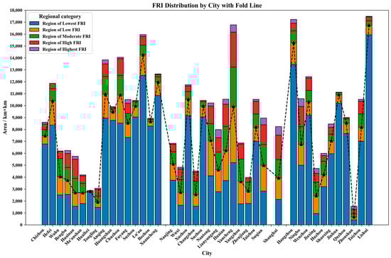
Figure 11.
FRI distribution by city, with fold line.
3.5. SHAP Results
3.5.1. Histogram of SHAP Values
In this study, the SHAP values of each metric across the nine sampling scenarios for risk prediction were calculated and presented in bar charts. Additionally, line graphs were plotted with the mean SHAP value as the node, as shown in Figure 12. The three metrics with the highest mean SHAP values were DEM, RAIN, and NDVI, respectively. Among these, DEM consistently exhibited a mean absolute SHAP value close to or greater than 1 in all sampling scenarios, significantly influencing the model’s prediction results. This suggests that elevation is the primary factor affecting flood occurrence. Rainfall ranked second in importance, although its impact was somewhat limited due to the relatively small size of the study area, where rainfall anisotropy is not pronounced and thus does not emerge as the primary driver of flooding. The third most influential factor was NDVI, as vegetation cover plays a crucial role in influencing surface runoff, especially in relatively flat areas with minimal topographic relief.
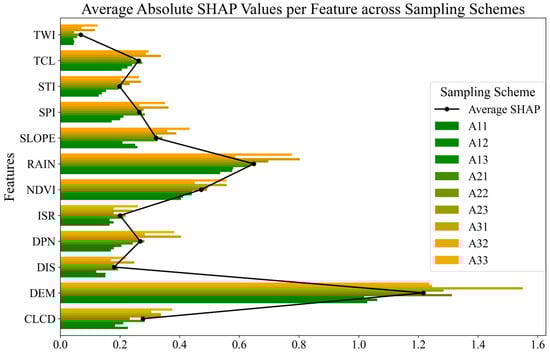
Figure 12.
Average absolute SHAP value.
3.5.2. Interaction Summary Plot
While the previous section highlighted the SHAP importance of each feature, this section focuses on the interactions between features, as shown in Figure 13. The plots on the diagonal (e.g., DEM–DEM, RAIN–RAIN) display the SHAP distribution of individual features, while the off-diagonal plots (e.g., DEM–RAIN, RAIN–NDVI) illustrate the interactions between pairs of features. The color gradient represents the feature values, with red indicating high values and blue indicating low values, which helps to visualize both the data distribution and the feature interactions. This study primarily analyzes the interactions of the three most influential indicators, based on their SHAP contributions. Given that the CLCD value represents different land use types and does not directly influence flooding, it was excluded from the interaction map.
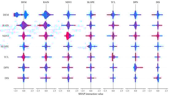
Figure 13.
SHAP indicator interactive chart. Red dots indicate samples with a large value for this characteristic (i.e., the indicator value is close to the maximum) and blue dots indicate samples with a small value for this characteristic (i.e., the indicator value is close to the minimum).
The DEM itself (DEM–DEM) shows a wide distribution of SHAP values, indicating that it has a significant influence on the model. High values (red) correspond to positive SHAP values, while low values (blue) have a negative contribution. A stronger interaction with RAIN suggests that topography significantly impacts rainfall accumulation (or runoff). The relatively weak interaction with NDVI and SLOPE is due to the limited direct relationship between elevation and vegetation (NDVI) or slope (SLOPE). The low interaction with TCL, DPN, and DIS indicates that the combined effect of elevation and these factors contributes less to the model’s prediction.
The RAIN itself (RAIN–RAIN) has a wide, asymmetrical SHAP value distribution, indicating that rainfall is a key factor in the model. The strongest interaction with DEM suggests that both rainfall and topography are major contributors to flood duration (or risk) predictions. The moderate interaction with NDVI and SLOPE suggests that rainfall affects flood characteristics through vegetation cover or slope. The small interaction with TCL, DPN, and DIS indicates that rainfall has an indirect influence on downstream watershed characteristics or distance to rivers.
The distribution of NDVI is narrower and less influential, suggesting that vegetation cover plays a limited role and mainly serves as an indirect buffer against floods. The medium interaction with RAIN indicates that rainfall affects vegetated and non-vegetated areas differently. The weak interaction with DEM and SLOPE suggests limited direct interaction between vegetation and topography. The negligible interaction with TCL, DPN, and DIS further highlights that the contribution of vegetation indices to the combination of these features is minimal.
The DEM (digital elevation model) and RAIN (rainfall) are the core features for predicting flood risk and significantly affect the probability of flooding. Notably, the SHAP distribution of RAIN is wide and asymmetrical, with both high and low rainfall values spread across positive and negative impact areas. This suggests that the effect of rainfall on flood risk is non-linear. During the low rainfall phase (SHAP values close to zero or negative), rainfall has little effect on flood risk, and its impact on low-lying areas may be mitigated by natural drainage systems or reduced due to improved subsurface conditions (e.g., enhanced soil wetness and reduced soil transport). As rainfall increases to a critical level (medium rainfall), surface drainage and infiltration capacities become saturated, leading to a rapid rise in flood risk. In the high rainfall phase (dramatic increase in SHAP values), under extreme rainfall conditions, the flood risk surges sharply, with highly non-linear impacts. The surface’s destructive capacity is amplified as water volume increases.
4. Discussion
In this study, two models, XGBoost and LSTM, were applied to predict the risk of flood occurrence and flood duration, respectively, and more reasonable prediction results were obtained. Simultaneous prediction of potential risk-duration was achieved, which in turn led to an integrated pre-disaster and post-disaster hazard evaluation. The study breaks through the previous limitation of only assessing flood risk and provides some reference for future flood risk management.
4.1. Rationalization of the Resolution Used in the Current Study
There are currently some peer-researched cases that use 1000 m × 1000 m as their study resolution. In a machine learning-based flood sensitivity assessment study of the Yangtze River Basin, 1 km resolution DEM and meteorological data were used, and it was confirmed that the 1 km resolution could meet the accuracy requirements in regional scale flood sensitivity analysis, with relatively higher computational efficiency [15]. Another study applied to basin-scale flood modeling in the lower Yangtze River region looks at resampling the data resolution from 30 m to 1000 m and hydrological modeling separately, with the main considerations being extended flood simulation and meteorological matching [36]. Another study assessed extreme precipitation in the YRD region using a 1.5 km resolution convection-allowed regional climate model. The results show that the high-resolution model exhibits higher accuracy in simulating extreme precipitation events and provides strong support for flood forecasting [37].
In summary, the 1 km resolution is considered moderate resolution (MR), which is reasonable and efficient in capturing large-scale flood characteristics (e.g., overall inundation extent, basin-level risk zoning, regional hydrological variability). Moreover, it has to be admitted that a 1 km resolution may be too coarse when studying details such as micro-drainage within the city and neighborhood ponding.
Although the 1 km resolution meets the basic standard for flood risk prediction at the regional scale, as well as at the regional scale, there are significant limitations in urban scale applications, especially for fine-grained flood modeling and potential damage assessment. Firstly, the 1 km resolution cannot adequately capture micro-topographic variations, such as low-lying areas, drainage outlets, under bridges, and other detailed areas, within the city, and these are often critical points for flood water accumulation. These micro-topographic changes in the city directly affect the distribution of water flow and the depth of water accumulation and therefore, cannot be accurately modeled at a 1 km resolution, which may lead to underestimation or under-reporting of local flood risks. Secondly, the 1 km resolution is also unable to accurately simulate the drainage systems, pumping stations, ditches, and other infrastructures within the city, and these play a crucial role in the mitigation of urban flooding and the guidance of water flows. For example, factors such as the layout of the urban drainage network, the drainage capacity, and the capacity of the pumping station cannot be accurately reflected at such a coarse resolution, which affects the accuracy of flood simulation. In addition, information such as the density of buildings and the degree of hardening of ground surfaces, which are crucial for the assessment of flood water accumulation and damage, cannot be adequately represented at a 1 km resolution. Due to the absence of these infrastructures and features, flood damage assessment may underestimate the actual risk, especially in critical areas such as residential, industrial, and utility areas. Finally, the large size of the 1 km resolution raster cells may result in some high-risk areas being misclassified as safe, or some areas that should be recognized as being affected by flooding being overlooked due to the “averaging effect”, thus affecting the accurate assessment of flood risk. In summary, although a 1 km resolution is suitable for large-scale flood risk assessment, in urban flood modeling and detailed damage assessment, in order to improve the accuracy of prediction and damage assessment, there is still a need to use higher resolution data (e.g., 10 m or 30 m resolution), combining it with more detailed engineering infrastructure data for multiscale modeling in order to more accurately reflect the complexity of the inner city and the role of flood defenses.
4.2. SHAP-Based Indicator Correlation Analysis
In this study, XGBoost and LSTM models are analyzed separately using SHAP to investigate the influence of various factors on flooding. SHAP enables the researcher to identify the most important features within each model and to explore interactions among them. This enhances our understanding of how these features collectively affect prediction outcomes. For decision makers, this approach offers a more transparent modeling process and valuable insights into the mechanisms behind flood prediction. Additionally, SHAP’s visualizations help present results in a clear and accessible format, which supports model optimization and the development of emergency response strategies.
However, different machine learning models can yield varying interpretation results due to the degree of compatibility with SHAP [38]. As a result, SHAP’s interpretive value remains somewhat limited and should be viewed as a transitional tool for improving transparency in black-box models. In future research, it is important to address interpretation bias stemming from model differences. A more robust version of SHAP is needed to reduce or eliminate inconsistencies across models.
Interpretation outcomes can also be influenced by changes in sample conditions. Variations in data sources, feature distributions, time spans, or spatial coverage may affect SHAP’s ability to consistently reflect feature importance [13]. In flood prediction, regions with unique topographic or climatic characteristics—such as steep slopes or highly variable rainfall—can show strong influences on model outputs. Historical trends regarding water levels or precipitation also play a key role, but if such trends are underrepresented in the training data, the model may fail to capture their full effects. In these cases, SHAP may not adequately reveal critical temporal dependencies. Furthermore, geographic differences significantly affect SHAP interpretation. For example, in mountainous regions where flash floods are common, soil and land use may be the dominant drivers. In contrast, in flat or coastal areas, where urban flooding or riverine inundation is more prevalent, elevation and rainfall tend to be more influential.
Similar conclusions have been reported in previous studies [15,17,39]. Moreover, research conducted in Poland using SHAP found that the main flood-driving factors were rainwater collectors, land surface temperature (LST), digital elevation model (DEM), soil type, river buffers, and the normalized difference vegetation index (NDVI) [40]. Another study identified rainfall as the primary driver of flooding [41]. In contrast, a study in South Korea highlighted land use and soil characteristics as the most significant contributors [42]. These differences are likely due to the geographic context of each study area. Flash flood-prone hillslopes may be more sensitive to soil and land use, while flat and coastal regions tend to be more affected by elevation and precipitation.
4.3. References for Flood Management
In this study, XGBoost is used as a decision tree model and LSTM as a time series model to predict flood risk and duration in the YRD. SHAP analysis revealed that the digital elevation model (DEM) is a key factor influencing flooding. This underscores the need to consider topography in urban planning, especially in the low-lying areas along the region’s rivers and coasts, which are particularly vulnerable to flooding. To mitigate this, flood protection measures in key cities like Shanghai, Nanjing, and Suzhou should be strengthened, focusing on the construction, operation, and maintenance of embankments, drainage systems, and flood protection infrastructure.
Flood management strategies in the YRD should be tailored to the region’s unique characteristics and evolving policy directions. Recently, more region-specific strategies have been implemented alongside sponge city initiatives. For example, Shanghai promotes a dual strategy of “sponge city + ocean city”, emphasizing the protection and restoration of marine ecosystems to address sea-level rise and extreme weather. Zhejiang has introduced a “green infrastructure + smart management” model for urban flood prevention, combining ecological wetlands and rain gardens with big data and AI for real-time monitoring and flood management. Meanwhile, Jiangsu focuses on integrating ecological restoration with cultural heritage in the design of waterfront spaces, enhancing both ecological quality and the preservation of historic sites.
Overall, the YRD is shifting from the traditional “hard defense” to a “soft defense” in regards to flood management. The focus is now on ecological restoration, smart management, and cultural integration, aiming for improved flood resilience and sustainable urban development.
4.4. Limitations
Flood occurrence is a complex and multifactorial process influenced by a wide range of climatic, geographic, hydrological, socioeconomic, and other factors. The flood prediction indicators used in this study are developed from four main dimensions: river, geography, vegetation, and subsurface characteristics. However, these factors alone are insufficient to fully capture the dynamics of flood occurrence. For instance, socioeconomic factors such as urbanization, river management practices, dyke construction, and land use changes may significantly impact the occurrence and propagation of floods. These factors are often not adequately represented in existing indicator systems. The lack of consideration of these non-natural influences may result in suboptimal model predictions, particularly in more complex scenarios.
In this study, the flood occurrence mechanism has been simplified to make the model more understandable and applicable. However, this simplification may overlook the intricate interactions between multiple factors, which could affect both the realism and the predictive accuracy of the model. For example, an increase in precipitation does not always directly result in flooding; factors such as soil infiltration capacity, river flow, and the effectiveness of regional flood defenses must also be taken into account. Existing flood prediction models are often constrained by specific spatial and temporal scales. Precipitation and watershed characteristics may change over short periods, but current models may not capture these rapid changes in real time. Moreover, the regional variability of rainfall in the study area is limited, which diminishes its impact on flood prediction. The scarcity of long-term meteorological and hydrological data in many areas, due to challenges in data acquisition, further limits the generalizability of models across different spatial and temporal contexts.
In flood prediction research, much of the focus has been on comparing several commonly used machine learning models (e.g., XGBoost, random forest, GBDT), while other potentially advantageous models (e.g., convolutional neural networks, generative adversarial networks) have often been overlooked. These models, particularly in deep learning, may offer distinct advantages in handling complex time-series data, non-linear relationships, or large-scale data. The limited selection of models in the current research may result in an incomplete evaluation of model performance, which in turn affects the accuracy of flood predictions. While existing models like XGBoost and LSTM have shown promising results, they do have certain limitations. XGBoost, for instance, can capture non-linear relationships between features but is constrained by its reliance on feature selection and tree structures, which makes it less effective in handling more complex feature interactions. LSTM, on the other hand, is adept at processing time-series data but displays limitations in modeling long-term dependencies. In these cases, emerging models, such as graph neural networks or deep reinforcement learning, may be better suited for capturing complex spatial and temporal dependencies. However, due to the limited scope of the model comparisons, the potential of these new models remains underexplored.
5. Conclusions
This study primarily uses XGBoost and LSTM to predict flood occurrence risk and flood duration, respectively, and proposes the flood risk index (FRI) as a composite indicator to measure the degree of flood hazard. A comparative analysis of the most critical indicators affecting floods was conducted using the SHAP interpreter. The main conclusions of this study are as follows.
- XGBoost exhibits the best performance in predicting flood occurrence risk. By comparing precision, recall, F1-score, accuracy, and AUC, XGBoost outperformed other models for all evaluation metrics, and the average multi-sample metric values (precision, recall, F1-score, accuracy, AUC) of XGBoost reached 0.823398, 0.831667, 0.827090, 0.826435, and 0.871062, respectively.
- High flood risk areas, long flood durations, and high FRI values are concentrated in large river basins and coastal areas. The study shows that flood risk ranges from 0.000073 to 0.998483, with a mean value of 0.237031; flood duration ranges from 0.223598 to 2.077040, with a mean value of 0.940050; and FRI ranges from 0 to 0.934256, with a mean value of 0.091711.
- From a provincial perspective, the provinces with the highest percentage of medium and high-value zones are Shanghai Municipality, Jiangsu Province, Anhui Province, and Zhejiang Province. Ten cities—Suzhou, Jiaxing, Yangzhou, Suqian, Changzhou, Wuxi, Lianyungang, Yancheng, Huai’an, and Bengbu—contain medium-high value zones exceeding 40%, with ratios of 48.99%, 48.07%, 46.87%, 44.19%, 43.43%, 43.20%, 42.21%, 40.88%, 40.73%, and 40.06%, respectively.
- SHAP interpreter analysis results indicate that elevation and rainfall are critical factors influencing flood occurrence. These two factors significantly affect the likelihood of flooding and should be key considerations in future flood management. In particular, the impact of elevation on flood risk should be fully addressed in urban planning, especially in coastal and floodplain areas, where flood protection infrastructure, such as dikes and urban drainage systems, is essential.
Author Contributions
Conceptualization, H.Z.; methodology, H.Z.; software, H.Z.; validation, K.Z. and Z.X.; data curation, X.J. and S.P.; writing—original draft preparation, H.Z.; writing—review and editing, X.W.; visualization, K.Z. and Z.X.; funding acquisition, X.W. All authors have read and agreed to the published version of the manuscript.
Funding
This research was funded by the National Key Research and Development Program of China, grant number 2016YFC0502700. The APC was funded by Fudan University.
Institutional Review Board Statement
Not applicable.
Informed Consent Statement
Not applicable.
Data Availability Statement
The data presented in this study are openly available in Global Flood Database, v1 (2000–2018), at https://doi.org/10.1038/s41586-021-03695-w, reference number [16].
Acknowledgments
All support has been acknowledged.
Conflicts of Interest
The authors declare no conflicts of interest.
Abbreviations
The following abbreviations are used in this manuscript:
| XGBoost | extreme gradient boosting |
| LSTM | long short-term memory |
| RF | random forest |
| GBDT | gradient boosted decision trees |
| FRI | flood risk index |
| YRD | Yangtze River Delta |
| DEM | digital elevation model |
| CLCD | Annual China Land Cover Dataset |
| SPI | stream power index |
| STI | sediment transport index |
| TWI | topographic wetness index |
| TCL | topographic control index |
| NDVI | normalized difference vegetation index |
| DIS | distance away from river |
| DPN | density of pipeline networks |
| ISR | impervious surface ratio |
| SHAP | Shapley additive explanations |
| AUC | area under the curve |
| ROC | receiver operating characteristic curve |
| MSE | mean squared error |
| MAE | mean absolute error |
| RMSE | root mean squared error |
| MAPE | mean absolute percentage error |
References
- Salman, M.; Li, Y. Flood Risk Assessment, Future Trend Modeling, and Risk Communication: A Review of Ongoing Research. Nat. Hazards Rev. 2018, 19, 4018011. [Google Scholar] [CrossRef]
- Sajid, T.; Maimoon, S.K.; Waseem, M.; Ahmed, S.; Khan, M.A.; Tränckner, J.; Pasha, G.A.; Hamidifar, H.; Skoulikaris, C. Integrated Risk Assessment of Floods and Landslides in Kohistan, Pakistan. Sustainablity 2025, 17, 3331. [Google Scholar] [CrossRef]
- Kumar, V.; Sharma, K.; Caloiero, T.; Mehta, D.J.; Singh, K. Comprehensive Overview of Flood Modeling Approaches: A Review of Recent Advances. Hydrology 2023, 10, 141. [Google Scholar] [CrossRef]
- Wu, X.; Zhu, H.; Hu, L.; Meng, J.; Sun, F. Analysis of Short-Term Heavy Rainfall-Based Urban Flood Disaster Risk Assessment Using Integrated Learning Approach. Sustainability 2024, 16, 8249. [Google Scholar] [CrossRef]
- Šiljeg, S.; Milošević, R.; Mamut, M. Pluvial Flood Susceptibility in the Local Community of the City of Gospić (Croatia). Sustainability 2024, 16, 1701. [Google Scholar] [CrossRef]
- Karymbalis, E.; Andreou, M.; Batzakis, D.-V.; Tsanakas, K.; Karalis, S. Integration of GIS-Based Multicriteria Decision Analysis and Analytic Hierarchy Process for Flood-Hazard Assessment in the Megalo Rema River Catchment (East Attica, Greece). Sustainability 2021, 13, 10232. [Google Scholar] [CrossRef]
- Fraehr, N.; Wang, Q.J.; Wu, W.; Nathan, R. Assessment of surrogate models for flood inundation: The physics-guided LSG model vs. state-of-the-art machine learning models. Water Res. 2024, 252, 121202. [Google Scholar] [CrossRef]
- Mosavi, A.; Ozturk, P.; Chau, K.-W. Flood Prediction Using Machine Learning Models: Literature Review. Water 2018, 10, 1536. [Google Scholar] [CrossRef]
- Wang, Z.L.; Lai, C.G.; Chen, X.; Yang, B.; Zhao, S.; Bai, X. Flood hazard risk assessment model based on random forest. J. Hydrol. 2015, 527, 1130–1141. [Google Scholar] [CrossRef]
- Tehrany, M.S.; Pradhan, B.; Mansor, S.; Ahmad, N. Flood susceptibility assessment using GIS-based support vector machine model with different kernel types. CATENA 2015, 125, 91–101. [Google Scholar] [CrossRef]
- Mojaddadi, H.; Pradhan, B.; Nampak, H.; Ahmad, N.; Ghazali, A.H.B. Ensemble machine-learning-based geospatial approach for flood risk assessment using multi-sensor remote-sensing data and GIS. Geomat. Nat. Hazards Risk 2017, 8, 1080–1102. [Google Scholar] [CrossRef]
- Zhao, G.; Pang, B.; Xu, Z.; Peng, D.; Xu, L. Assessment of urban flood susceptibility using semi-supervised machine learning model. Sci. Total Environ. 2019, 659, 940–949. [Google Scholar] [CrossRef]
- Chen, J.; Huang, G.; Chen, W. Towards better flood risk management: Assessing flood risk and investigating the potential mechanism based on machine learning models. J. Environ. Manag. 2021, 293, 112810. [Google Scholar] [CrossRef]
- Kanani-Sadat, Y.; Safari, A.; Nasseri, M.; Homayouni, S. A novel explainable PSO-XGBoost model for regional flood frequency analysis at a national scale: Exploring spatial heterogeneity in flood drivers. J. Hydrol. 2024, 638, 131493. [Google Scholar] [CrossRef]
- Zhu, K.; Wang, Z.; Lai, C.; Li, S.; Zeng, Z.; Chen, X. Evaluating Factors Affecting Flood Susceptibility in the Yangtze River Delta Using Machine Learning Methods. Int. J. Disaster Risk Sci. 2024, 15, 738–753. [Google Scholar] [CrossRef]
- Zhu, S.; Feng, H.; Shao, Q. Evaluating Urban Flood Resilience within the Social-Economic-Natural Complex Ecosystem: A Case Study of Cities in the Yangtze River Delta. Land 2023, 12, 1200. [Google Scholar] [CrossRef]
- Deng, M.; Li, Z.; Tao, F. Rainstorm Disaster Risk Assessment and Influence Factors Analysis in the Yangtze River Delta, China. Int. J. Environ. Res. Public Health 2022, 19, 9497. [Google Scholar] [CrossRef]
- Zhang, Y.; Yao, R.; Zhu, Z.; Jin, H.; Zhang, S. Spatiotemporal evolution of population exposure to multi-scenario rainstorms in the Yangtze River Delta urban agglomeration. J. Geogr. Sci. 2024, 34, 654–680. [Google Scholar] [CrossRef]
- Saha, A.; Chandra Pal, S. Application of machine learning and emerging remote sensing techniques in hydrology: A state-of-the-art review and current research trends. J. Hydrol. 2024, 632, 130907. [Google Scholar] [CrossRef]
- Tellman, B.; Sullivan, J.A.; Kuhn, C.; Kettner, A.J.; Doyle, C.S.; Brakenridge, G.R.; Erickson, T.A.; Slayback, D.A. Satellite imaging reveals increased proportion of population exposed to floods. Nature 2021, 596, 80–86. [Google Scholar] [CrossRef]
- Vanama, V.S.K.; Mandal, D.; Rao, Y. GEE4FLOOD: Rapid mapping of flood areas using temporal Sentinel-1 SAR images with Google Earth Engine cloud platform. J. Appl. Remote Sens. 2020, 14, 034505. [Google Scholar] [CrossRef]
- Bui, Q.D.; Luu, C.; Mai, S.H.; Ha, H.T.; Ta, H.T.; Pham, B.T. Flood risk mapping and analysis using an integrated framework of machine learning models and analytic hierarchy process. Risk Anal. 2023, 43, 1478–1495. [Google Scholar] [CrossRef] [PubMed]
- Liu, Z.; Felton, T.; Mostafavi, A. Interpretable machine learning for predicting urban flash flood hotspots using intertwined land and built-environment features. Comput. Environ. Urban Syst. 2024, 110, 102096. [Google Scholar] [CrossRef]
- Fang, Z.; Wang, Y.; Peng, L.; Hong, H. Predicting flood susceptibility using LSTM neural networks. J. Hydrol. 2021, 594, 125734. [Google Scholar] [CrossRef]
- Huang, H.; Chen, X.; Wang, X.; Wang, X.; Liu, L. A Depression-Based Index to Represent Topographic Control in Urban Pluvial Flooding. Water 2019, 11, 2115. [Google Scholar] [CrossRef]
- Chen, T.; Guestrin, C. XGBoost: A Scalable Tree Boosting System. In Proceedings of the 22nd ACM SIGKDD International Conference on Knowledge Discovery and Data Mining, San Francisco, CA, USA, 13–17 August 2016. [Google Scholar] [CrossRef]
- Dtissibe, F.Y.; Ari, A.A.A.; Abboubakar, H.; Njoya, A.N.; Mohamadou, A.; Thiare, O. A comparative study of Machine Learning and Deep Learning methods for flood forecasting in the Far-North region, Cameroon. Sci. Afr. 2024, 23, e02053. [Google Scholar] [CrossRef]
- Atashi, V.; Kardan, R.; Gorji, H.T.; Lim, Y.H. Comparative Study of Deep Learning LSTM and 1D-CNN Models for Real-time Flood Prediction in Red River of the North, USA. In Proceedings of the 2023 IEEE International Conference on Electro Information Technology (eIT), Romeoville, IL, USA, 18–20 May 2023. [Google Scholar] [CrossRef]
- Le, X.-H.; Nguyen, D.-H.; Jung, S.; Yeon, M.; Lee, G. Comparison of Deep Learning Techniques for River Streamflow Forecasting. IEEE Access 2021, 9, 71805–71820. [Google Scholar] [CrossRef]
- Rahimzad, M.; Moghaddam Nia, A.; Zolfonoon, H.; Soltani, J.; Mehr, A.D.; Kwon, H.-H. Performance Comparison of an LSTM-based Deep Learning Model versus Conventional Machine Learning Algorithms for Streamflow Forecasting. Water Resour. Manag. 2021, 35, 4167–4187. [Google Scholar] [CrossRef]
- Khairudin, N.B.M.; Mustapha, N.B.; Aris, T.N.B.M.; Zolkepli, M.B. Comparison of Machine Learning Models For Rainfall Forecasting. In Proceedings of the 2020 International Conference on Computer Science and Its Application in Agriculture (ICOSICA), Bogor, Indonesia, 16–17 September 2020. [Google Scholar] [CrossRef]
- Hochreiter, S.; Schmidhuber, J. Long Short-Term Memory. Neural Comput. 1997, 9, 1735–1780. [Google Scholar] [CrossRef]
- Qi, M.; Huang, H.; Liu, L.; Chen, X. An Integrated Approach for Urban Pluvial Flood Risk Assessment at Catchment Level. Water 2022, 14, 2000. [Google Scholar] [CrossRef]
- Apel, H.; Martínez Trepat, O.; Hung, N.N.; Chinh, D.T.; Merz, B.; Dung, N.V. Combined fluvial and pluvial urban flood hazard analysis: Concept development and application to Can Tho city, Mekong Delta, Vietnam. Nat. Hazards Earth Syst. Sci. 2016, 16, 941–961. [Google Scholar] [CrossRef]
- Sanders, W.; Li, D.; Li, W.; Fang, Z.N. Data-Driven Flood Alert System (FAS) Using Extreme Gradient Boosting (XGBoost) to Forecast Flood Stages. Water 2022, 14, 747. [Google Scholar] [CrossRef]
- Chen, Z.; Zeng, Y.; Shen, G.; Xiao, C.; Xu, L.; Chen, N. Spatiotemporal characteristics and estimates of extreme precipitation in the Yangtze River Basin using GLDAS data. Int. J. Climatol. 2021, 41, E1812–E1830. [Google Scholar] [CrossRef]
- Dong, G.; Jiang, Z.; Wang, Y.; Tian, Z.; Liu, J. Evaluation of extreme precipitation in the Yangtze River Delta Region of China using a 1.5 km mesh convection-permitting regional climate model. Clim. Dyn. 2022, 59, 2257–2273. [Google Scholar] [CrossRef]
- Zhao, J.C.; Zhang, C.B.; Wang, J.; Abbas, Z.; Zhao, Y. Machine learning and SHAP-based susceptibility assessment of storm flood in rapidly urbanizing areas: A case study of Shenzhen, China. Geomat. Nat. Hazards Risk 2024, 15, 2311889. [Google Scholar] [CrossRef]
- Wang, Q.; Xu, Y.; Wang, J.; Lin, Z.; Dai, X.; Hu, Z. Assessing sub-daily rainstorm variability and its effects on flood processes in the Yangtze River Delta region. Hydrol. Sci. J. 2019, 64, 1972–1981. [Google Scholar] [CrossRef]
- Gulshad, K.; Yaseen, A.; Szydłowski, M. From Data to Decision: Interpretable Machine Learning for Predicting Flood Susceptibility in Gdańsk, Poland. Remote Sens. 2024, 16, 3902. [Google Scholar] [CrossRef]
- Starzec, M.; Kordana-Obuch, S. Evaluating the Utility of Selected Machine Learning Models for Predicting Stormwater Levels in Small Streams. Sustainability 2024, 16, 783. [Google Scholar] [CrossRef]
- Pradhan, B.; Lee, S.; Dikshit, A.; Kim, H. Spatial flood susceptibility mapping using an explainable artificial intelligence (XAI) model. Geosci. Front. 2023, 14, 101625. [Google Scholar] [CrossRef]
Disclaimer/Publisher’s Note: The statements, opinions and data contained in all publications are solely those of the individual author(s) and contributor(s) and not of MDPI and/or the editor(s). MDPI and/or the editor(s) disclaim responsibility for any injury to people or property resulting from any ideas, methods, instructions or products referred to in the content. |
© 2025 by the authors. Licensee MDPI, Basel, Switzerland. This article is an open access article distributed under the terms and conditions of the Creative Commons Attribution (CC BY) license (https://creativecommons.org/licenses/by/4.0/).