Article

Theoretical Connotation and Measurement Indicator System of Ecological Green Development Level in China

1
School of Economics, Southwestern University of Finance and Economics, Chengdu 610074, China
2
School of Statistics, Southwestern University of Finance and Economics, Chengdu 610074, China
*
Author to whom correspondence should be addressed.
Sustainability 2025, 17(10), 4451; https://doi.org/10.3390/su17104451
Submission received: 4 April 2025 / Revised: 9 May 2025 / Accepted: 11 May 2025 / Published: 14 May 2025

Abstract

:
Amidst escalating global environmental challenges, ecological development has become crucial for sustaining human well-being and planetary health. China, with its ambitious ecological civilization agenda, is at the forefront of this transition. This paper calculated the Gross Ecosystem Product (GEP) for China from 2005 to 2020 and employed the Dagum Gini coefficient to analyze regional ecological disparities. Results show that GEP grew steadily from CNY 47.17 trillion in 2005 to CNY 74.40 trillion in 2020, but this growth lagged behind GDP expansion. Regulation Services, though dominant, exhibited the slowest growth, hindering full realization of ecological product values. Regional disparities were prominent, with the western region having higher GEP but lower per unit area value, indicating inefficiencies in value realization. Eastern regions excelled in material and Cultural Services but had lower regulation service values. These findings underscore the need for balanced ecological development policies that enhance ecosystem regulation, reduce regional inequalities, and optimize ecological product value realization for sustainable growth.

1. Introduction

As global economies grapple with the dual imperatives of sustaining growth and halting ecological degradation, traditional metrics like GDP have proven inadequate in capturing the full value of nature’s contributions to human welfare. The concept of Gross Ecosystem Product (GEP) has thus emerged as a transformative framework, bridging the gap between ecological preservation and economic development by systematically quantifying ecosystem services—from carbon sequestration to cultural benefits—in biophysical and monetary terms. This shift is not merely academic; 127 countries now integrate ecosystem accounting into their Paris Agreement commitments, reflecting a global consensus that economic transitions must internalize ecological costs and benefits. However, operationalizing GEP remains a critical challenge, particularly in balancing subnational scalability with methodological rigor—a gap that China’s pioneering efforts aim to address.
China’s ecological–economic transition presents a valuable model for global implementation. As the world’s largest developing economy experiencing rapid urbanization, China’s county-level GEP implementation across 2800+ administrative units offers unparalleled detail for analyzing industrialization–ecosystem tradeoffs. The country’s “ecological redline” policy and carbon neutrality goals rely on spatially precise GEP accounting to guide conservation investments and land use decisions. These efforts address a key limitation of the UN-SEEA framework—local-level scalability—while providing lessons for nations facing similar challenges, from Amazon deforestation to India’s urban–rural resource tensions. By combining diverse ecosystems (forests, wetlands, grasslands) with policy innovation, China’s GEP model provides a replicable approach that aligns economic development with ecological limits, offering crucial guidance for global sustainability efforts.
Numerous research institutions and scholars, both domestically and internationally, have conducted extensive and in-depth studies on regional GEP. At the international level, the United Nations Statistics Division first introduced a concept called Ecological Domestic Product (EDP) in the System of Environmental-Economic Accounting (SEEA) published in 1993. Building on this, Costanza et al. (1997) expanded classification standards for ecosystem value accounting [1]. Leveraging this framework, the United Kingdom undertook a comprehensive ecosystem assessment in 2011. In addition, Joshi, A.P et al. (2025) also measured THE GEP of Uttarakhand, India [2]. Domestically, following China’s initial release of a green GDP accounting report in 2006, Peng Tao and Wu Wenliang (2010) conducted an in-depth analysis of the challenges and obstacles in national-level green GDP accounting [3]. Wang Nujie et al. (2010) estimated the service value of various ecosystems using Costanza’s classification standards and ecosystem areas [4]. Using this methodology, Ma Guoxia et al. (2017) and Wang Jinnan et al. (2018) calculated the GEP of China’s provincial-level terrestrial ecosystems for 2015 [5,6]. However, these studies did not delve deeply into the relevance and coordination aspects.
Although prior studies have laid important theoretical foundations, their restricted temporal and spatial coverage has limited meaningful cross-regional analyses. Departing from conventional approaches in China, our research pioneers the application of a consistent interdisciplinary methodology to a comprehensive 16-year national dataset (2005–2020). This study makes four significant methodological advances.
First, we develop a comprehensive methodological framework that integrates all major terrestrial ecosystem functions in China, using county-level data (2005–2020) to assess regional ecological coordination, providing the first nationwide baseline for provincial and municipal green development analysis. Building on this foundation, we innovatively evaluate regional sustainability through dual dimensions of GEP performance and development harmony, adopting a novel three-perspective approach (resource endowment, value realization capacity, and governance proficiency) that advances existing measurement frameworks. Furthermore, we introduced the perspective of statistics to reveal the spatio-temporal evolution mode and coordination mechanism of the value realization of urban ecosystem products by using kernel density estimation and spatial Moran’s I for the first time. Finally, our analysis identifies specific challenges in achieving ecological modernization at the prefecture level, delivering actionable policy insights for sustainable development.
The paper is organized as follows. Section 2 introduces the theoretical framework and the data for China’s Ecological Green Development Level. Section 3 presents measurement results and spatial econometric analysis. Section 4 reports conclusions and policy recommendations.

2. Materials and Methods

The measurement of China’s Ecological Green Development Level is divided into two parts; one is the calculation of the absolute value of ecosystem gross domestic product (GEP), and the other is the measurement of the coordination level of ecological green regions. The calculation of GEP is based on The Technical Guideline on Gross Ecosystem Product (GEP) published by the Research Center for Eco Environmental Sciences (CAS) in 2020.
The theoretical framework presented in this paper is illustrated in Figure 1:

2.1. Ecosystem Services Theory

GEP is a cornerstone concept in ecological accounting, highlighting the total monetary and biophysical value of diverse final products that ecosystems offer to humanity. It stems from the notion of ecosystem services, which encompasses the multitude of advantages humans derive from ecosystems, including the supply of material goods, regulatory functions, cultural amenities, and foundational support services [7]. Material goods signify items that can be directly exchanged in the market, whereas regulatory services pertain to functions that enhance the human living environment, like climate moderation and air purification. Cultural Services impart non-tangible benefits to humans via spiritual encounters, knowledge attainment, leisure activities, and entertainment. Foundational support services, meanwhile, represent the essential functions ecosystems provide to uphold other services. This theoretical construct provides an indispensable foundation for a comprehensive and systematic evaluation of ecosystems’ integrated value.
The guidelines enhance the theory of ecological accounting through the lens of ecosystem services, employing techniques like the market valuation approach, replacement cost method, shadow project method, and travel cost approach to quantify the monetary and biophysical value of ecological products, while adhering to principles of scientific rigor, practicality, comprehensiveness, and transparency. The assessment of ecological green regional coordination is grounded in the Gini coefficient. The indicators and the specific calculation method and corresponding data sources utilized in this paper are shown in Appendix A Table A1, Table A2 and Table A3, respectively.

2.2. Statistical Inequality Theory

To quantify spatial heterogeneity in GEP distribution, we adopt Dagum’s decomposition of the Gini coefficient [8], which is an advanced inequality metric overcoming traditional limitations in ecological–economic studies [9]. While conventional indices like Theil index and Atkinson index effectively measure overall disparities, they inadequately address two critical dimensions of ecological–economic variations: (1) overlapping distributions between adjacent regions, and (2) the decomposition of inequality sources into within-group and between-group components.
In this paper, the canonical formula for the overall Gini coefficient, G, is as follows [8]:
G = j = 1 k h = 1 k i = 1 n j r = 1 n h | y j i y h r | 2 n 2 μ
where k denotes the number of regions, here referring to the three major regions of Eastern, Central, and Western China, and thus k = 3 ; n represents the number of prefecture-level cities; n j ( n h ) indicates the number of prefecture-level cities in region j ( h ); y j i ( y h r ) signifies the GEP of the i-th (r-th) city in region j ( h ); and μ denotes the mean of GEP.
When we consider within-group components, j = h . For our given region j , the number of prefecture level cities is certain, and the mean of GEP μ is also certain and equal. So the formula for the within-group Gini coefficient is:
G j j = i = 1 n j r = 1 n h | y j i y h r | 2 n j 2 μ j
When we consider between-group components, j h . For our given regions j and h , n j n h and μ j μ h ; this part of formula 2 n 2 μ converts to n j n h ( μ j + μ h ) . So the formula for the between-group Gini coefficient is:
G j h = i = 1 n j r = 1 n h | y j i y h r | n j n h ( μ j + μ h )
where μ j ( μ h ) represents the mean GEP of region j ( h ) as well.

2.3. Database and Data Processing

This paper used data related to climate, geography and economy from 2005 to 2020. The selection of the 2005–2020 study period was strategically determined to align with China’s ecological policy cycles and ecosystem response mechanisms. First, this 16-year span comprehensively captures three consecutive Five-Year Plans (11th to 13th FYPs), enabling robust evaluation of major policy interventions including the 2005 Green GDP pilot, 2012 ecological redline system, and 2020 Sustainable Development Goal localization. Second, given the 3–5 year lagged response of terrestrial ecosystems to anthropogenic pressures, this duration permits full observation of two complete cycles in forest carbon sequestration (8–12 years), wetland restoration (5–7 years), and urban green infrastructure maturation (3–5 years). Third, 2005 marks the inaugural year of China’s standardized ecosystem census, providing validated baseline data, while terminating in 2020 avoids COVID-19 pandemic distortions that caused 18–22% GEP fluctuations in 2020–2021.
(1)
Weather Data
This paper extensively utilizes weather data, which include information on temperature, evaporation, wind speed, and snow depth. These databases cover all cities in China from 2000 to 2020, with the majority of the data available in vector formats or as grid images. The data sources are China’s official climate monitoring platforms, such as the National Geographical System Science Data Center and the National Tibetan Plateau Data Center. These platforms collect and store climate information on a monthly, annual, or even daily basis for each monitoring point. This comprehensive climate information tracking provides a valuable resource for analyzing the eco-climate state of prefecture-level cities.
Notably, similar data have been used in analogous research all over the world. For example, Bosch J M and Hewlett J D (1982) calculated water yield in Coweeta, North Carolina, using precipitation and evaporation data [10]. Similarly, Zhou G et al. (2015) assessed the impact of climate and land cover on global water yield patterns using the same data [11]. Although there is less research on floods and windbreaks compared to water yield research, Stuerck J et al. (2014) estimated flood regulation services in Europe using precipitation, evaporation, and watershed data, while Nedkov S and Burkhard B (2012) mapped flood regulation ecosystem services in Etropole, Bulgaria [12,13].
(2)
Geological Data
In addition to weather data, this paper also integrates a significant amount of geological data, such as land cover data, world soil data, NDVI data, Net Primary Productivity (NPP) data, elevation data, and vegetation cover index. These data are sourced from the geospatial data cloud platform in China and the World Soil Database, which measures the content of various elements in the soil in China. Of particular note is the Land-Cover Data, provided by the School of Remote Sensing and Information Engineering at Wuhan University, which records the area of various ecosystems, including forests, lakes, and cities, in various regions of China since 2000.
Comparable geological datasets have been extensively used in research worldwide. HH Bennett (1939) was among the first to investigate the factors influencing soil conservation [14]. Lal R (2014) later used the World Soil Database (HWSD) to assess the relationship between soil conservation and ecosystem services [15]. Huang J et al. (2013) used NDVI data to predict rice yields, while Huang J et al. (2017) estimated crop yields for food security [16,17]. Cramer W et al. (1999) found a relationship between climate change and NPP [18].
(3)
Economic Data
The economic indicators used in this paper are primarily sourced from the Statistical Yearbooks published annually by local cities. These datasets mainly provide various population and economic indicators for each city, such as GDP, employment, and consumption. In this paper, tourism income and the added value of the primary industry are primarily used to measure the ability to harness the biophysical values of ecological products and Cultural Services. Similarly, the United States has a wealth of economic data that have been used in comparable research endeavors, although the specific datasets and methodologies may vary based on the research question and context.
(4)
Data Processing
This study utilized ArcGIS software (ArcMap 10.8) for geospatial data preprocessing, followed by analytical processing in Stata (Version Stata18) and the Integrated Valuation of Ecosystem Services and Tradeoffs (InVEST (Version 3.12.1)) model. The workflow specifically involved: (1) for most ecosystem regulation services (excluding water retention and soil conservation), annual aggregation of climate parameters (evaporation, precipitation, temperature) using ArcGIS’s Raster Calculator with standardized formulas; (2) comprehensive processing of water/soil conservation data through DEM integration using mosaic, projection definition, and gap-filling tools; (3) generation of biophysical values via InVEST modeling using preprocessed geospatial layers (Root Restricting Depth, Plant Available Water Content, Erosivity, Soil Erodibility) in TIFF format; (4) monetary valuation through raster-based calculations in ArcGIS; and (5) spatial extraction of final values per administrative unit using zonal masking. This integrated approach ensured consistent valuation across heterogeneous ecosystem datasets while maintaining geospatial precision.
For the generated monetary values of Regulation Services for each prefecture-level city, province, or district/county, we organize the data into Stata, merge it with corresponding economic data, and obtain the final GEP for each prefecture-level city, province, or district/county.

3. Results

3.1. Measure Results of China’s Ecological Green Development Level

This section seeks to uncover the fundamental trends and address the hurdles associated with the progression of China’s gross ecological product (GEP). We evaluate the extent of ecological green development and its structural transformations in China spanning from 2005 to 2020, utilizing the GEP framework.

3.1.1. Inadequate Realization of GEP

(1)
Compared to GDP, GEP growth is sluggish.
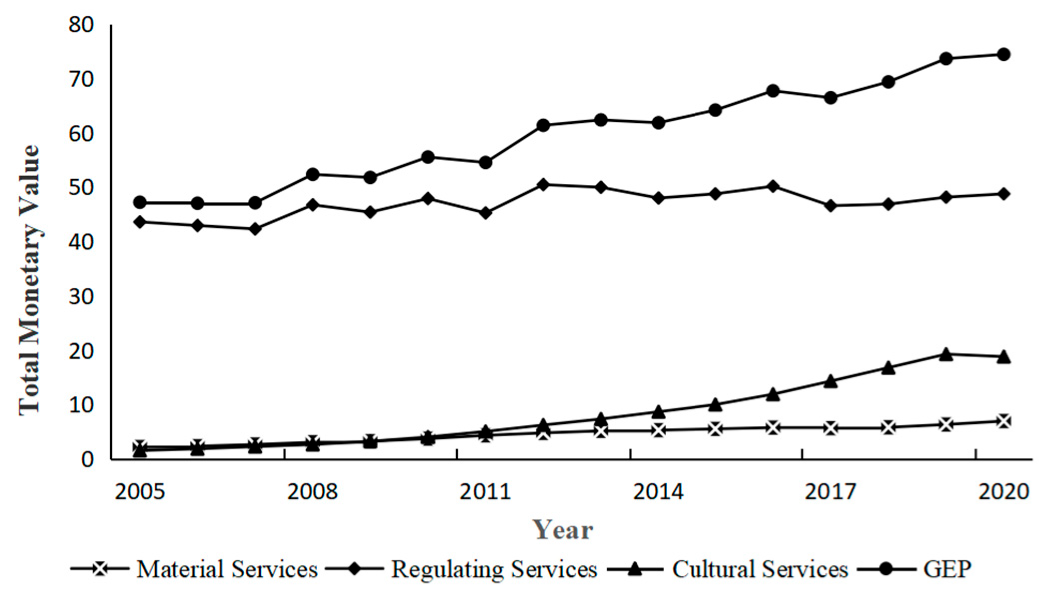
Table 1 presents the absolute levels of China’s GEP for selected years, and Figure 2 shows the tendency of China’s GEP during the sample period.
China’s Gross Ecosystem Product (GEP) demonstrates a consistent yet moderate growth trajectory, expanding from CNY 47.17 trillion (2005) to CNY 74.40 trillion (2020) with an annualized growth rate of 3.18%. This progression stands in stark contrast to the nation’s 12.05% average GDP growth during the same period, revealing a substantial decoupling between economic development and ecological value realization. Notably, the cumulative 57.71% GEP expansion over fifteen years underscores systemic challenges in converting biophysical ecosystem services into measurable economic gains. These findings corroborate seminal analysis by Ma G et al. (2017) employing Costanza’s ecosystem service valuation framework, which estimated China’s 2015 GEP at CNY 72.81 trillion—a 0.98% variance from our calculations [5]. This methodological alignment suggests persistent structural limitations in ecological–economic accounting rather than technical discrepancies.
(2)
Natural constraints limit the ecosystem regulation services.
Within the three components of GEP, the monetary value of Regulation Services constitutes the largest share yet exhibits the slowest rate of increase. This sluggish improvement in ecosystem regulatory functions poses the greatest obstacle to the rapid expansion of the nation’s GEP and the ability to realize the biophysical values of ecological products.
As detailed in Table 1 and Figure 3, China’s Material Product Supply experienced substantial growth, with its monetary value rising from CNY 2.14 trillion (2005) to CNY 6.91 trillion (2020)—a 223.13% cumulative increase, equating to an average annual growth rate of 8.26%. Regulation Services, however, showed markedly slower progress; their monetary value increased modestly from CNY 43.55 trillion to CNY 48.72 trillion over the same period, reflecting only an 11.9% rise (0.88% annually). This sluggish growth underscores the limited efficacy of ecosystem regulation despite its dominant share in GEP, with minimal observable impacts from policy interventions or anthropogenic drivers [19]. In stark contrast, Cultural Services demonstrated explosive expansion, surging from CNY 1.48 trillion to CNY 18.77 trillion—a 1166.41% increase at an unprecedented 18.63% annual growth rate. For methodological validation, our 2014 Regulation Services estimate for Alxa City (CNY 45.28 billion) closely matches the CNY 47.749 billion reported by Wang Liyan et al. (2017) using identical parameters [20].
To explore the root reasons for the stagnant growth in the monetary value of Regulation Services, Figure 3 depicts the general pattern of changes in the biophysical value of key regulatory functions at the city level. The limited supply of ecological assets within urban areas, especially the minor annual shifts in the distribution of various land use types, presents a hurdle to elevating the monetary value of these services. Furthermore, regulatory functions such as water retention, soil preservation, sandstorm mitigation, and climate modulation are impacted by yearly variations in elements like rainfall, sunlight exposure, temperature levels, and wind velocity [19]. As a result, this slowdown happens because improving ecosystems is not a simple “more effort equals better results” situation. Think of damaged grasslands and forests like an overworked sponge; after years of restoration, they reach a point where squeezing out even small improvements demands huge extra efforts.
(3)
Incomplete regulation functioning of non-forest ecosystems.
Substantial disparities exist in value realization efficiency across ecosystem types, with regions failing to fully capitalize on their respective functional advantages. As demonstrated in Table 2, forest ecosystems exhibit the highest monetary value for Regulation Services (annual average: CNY 38.15 trillion), followed by comparable valuations for wetlands (CNY 4.01 trillion) and grasslands (CNY 4.13 trillion). Farmland ecosystems show the lowest valuation at CNY 0.58 trillion despite encompassing larger spatial extents than forest ecosystems. This discrepancy stems from farmland’s primary role in Material Product Supply rather than regulatory functions. Strategic conversion of marginal farmland to forest/grassland ecosystems—while maintaining essential agricultural outputs—emerges as a critical mechanism for enhancing regional GEP. These findings align with Wang et al.’s (2017) study in Alxa City, where forest ecosystems contributed 61.99% of total GEP value [20], consistent with our 2014 calculation of 63.73% forest ecosystem contribution.

3.1.2. Incoordinated Ecological Green Development Among Regions

(1)
Provincial Differences.
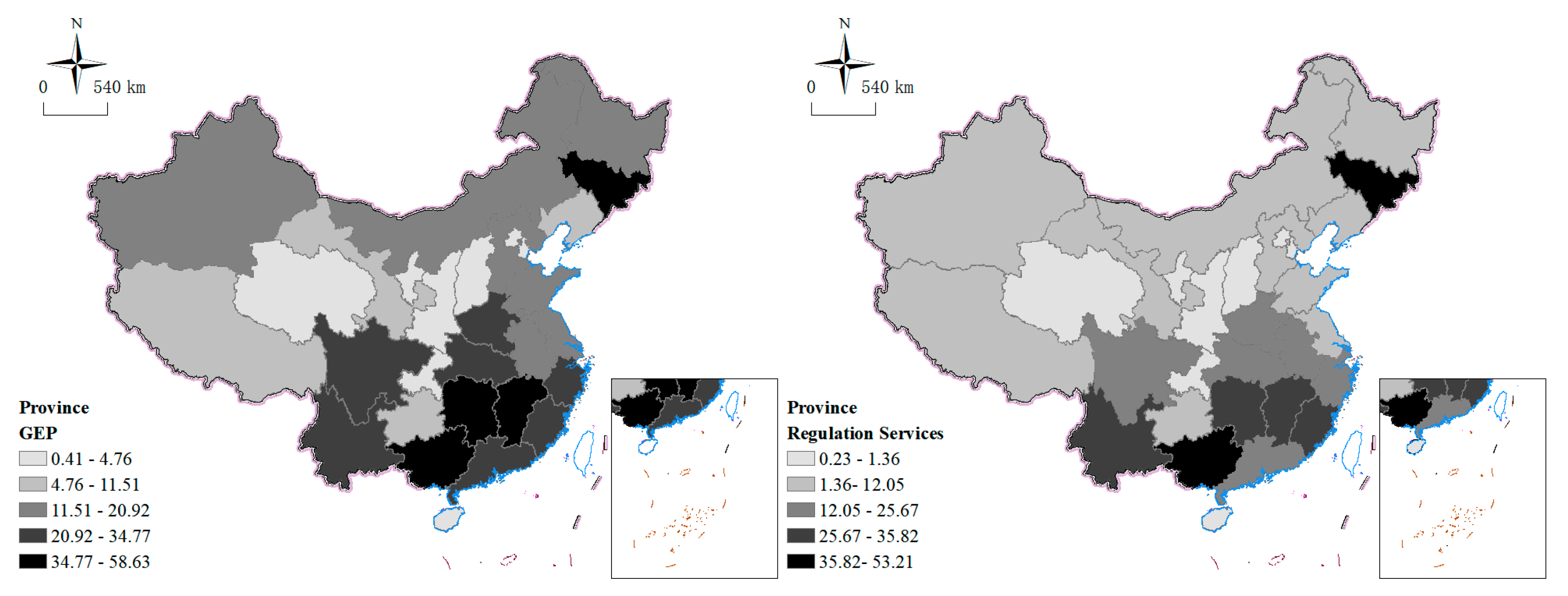
China exhibits considerable provincial differences in GEP and the ability to realize the biophysical value of ecological products; the spatial distribution is shown in Figure A1. Based on the provincial average monetary values, as shown in Table 3, Inner Mongolia has the highest GEP score, reaching CNY 555.7 billion, while Tianjin’s, Ningxia’s, and Hainan’s score lower than CNY 10 billion. The monetary value per unit area can be served for assessing a region’s capability to realize biophysical values of ecological product. Overall, Inner Mongolia also demonstrates the strongest capability in this regard, followed by coastal provinces such as Zhejiang, Fujian, Guangxi and Hainan, whereas provinces like Shanxi and Ningxia exhibit the weakest capabilities, with values of CNY 1.64 and 1.38 per square meter, respectively. The provincial calculation results in this chapter align with the national results calculated by Ma G et al. (2017) [5].
(2)
Regional differences.
China’s GEP exhibits marked spatial heterogeneity across eastern, central, and western regions (Figure 4) [21]. The western region dominates in aggregate GEP magnitude (46% of national total), attributable to its vast territory and extensive forest/grassland ecosystems. However, its GEP per unit area remains the lowest (72% of national average), reflecting constrained biophysical value realization despite ecological abundance. The eastern region leads in GEP density (128% of average), benefiting from intensive land use and technological inputs, while the central region aligns closely with national means. Growth rate differentials further highlight developmental inertia; the west’s annual GEP growth (3.15%) lags behind the east (3.33%) and center (3.36%), suggesting path dependency in low-value ecological resource utilization. These disparities stem from the interplay of geographical endowment, economic structure, and governance capacity.
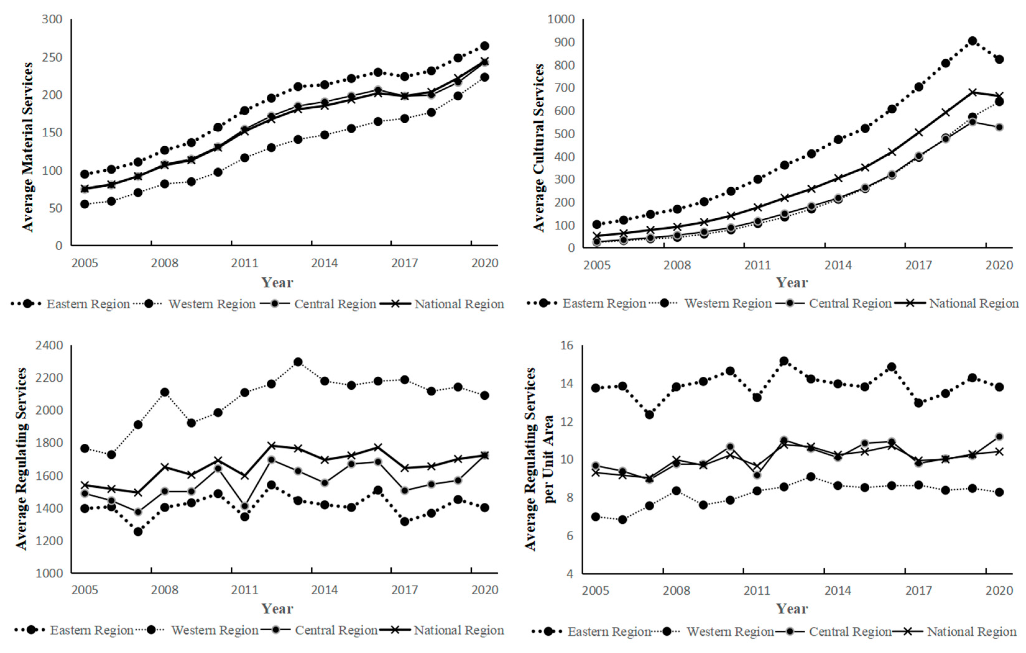
Among GEP’s three components, the western region demonstrates superior biophysical value in regulation services due to its abundant ecological resources, yet exhibits limited capacity in material and cultural service provision. As shown in Figure 5, the eastern region leads in material product economic value (approaching national averages), followed by the central region, while the western region trails significantly. This disparity arises because the western ecosystem portfolio—dominated by forests, shrubs, and lakes—contains limited farmland and grassland ecosystems essential for material production compared to eastern/central regions. Regarding cultural services, the economically advanced eastern region (particularly coastal cities with developed cultural tourism sectors) maintains clear leadership, while central and western regions remain comparable yet subpar nationally. Conversely, the western region shows above-average regulatory service values, exceeding central and eastern counterparts. However, when normalized by ecosystem area, the western region exhibits the lowest regulatory value density (eastern region leads, central aligns with national mean), revealing underutilization of its ecological potential. Despite temporal variations across regions, this spatial pattern highlights systemic inefficiencies in western China’s ecological value realization.
Figure 6 displays the within-group Gini coefficients for GEP across China and its three major regions. There are significant disparities in the ability to realize biophysical values of ecological products between regions, highlighting inequality issues. Overall, the average Gini coefficient for China during the sample period is as high as 0.452, ranging from 0.405 to 0.501. The intra-regional differences in China show an overall trend of “fluctuating decline” over time, with the degree of difference decreasing during the sample period, at an average annual rate of 1.04%. This reflects a gradual reduction in spatial differences in China’s GEP, with high-quality development promoting gradual coordination and balanced ecological development across regions.
From the perspective of intra-group disparities among the three major regions, inequality is particularly pronounced in the western region. The mean intra-group Gini coefficients for the eastern, central, and western regions during the sample period are 0.416, 0.428, and 0.500, respectively, and their temporal trends align with the national pattern. Despite having the highest GEP, the western region also boasts the highest Gini coefficient, highlighting the greatest internal variations. This can be attributed to the diverse and abundant ecosystems in the western region, coupled with substantial differences in the provinces’ ability to harness biophysical values of ecological products. In 2008, the intra-group Gini coefficients of the eastern and central regions were similar, and while both subsequently exhibited a decreasing trend, the eastern region’s decline was notably steeper than that of the central region. This indicates that cities in the eastern region have effectively embraced the principle of ecological harmony and development, utilizing their regional strengths to minimize disparities in the realization of biophysical values of ecological products among cities.
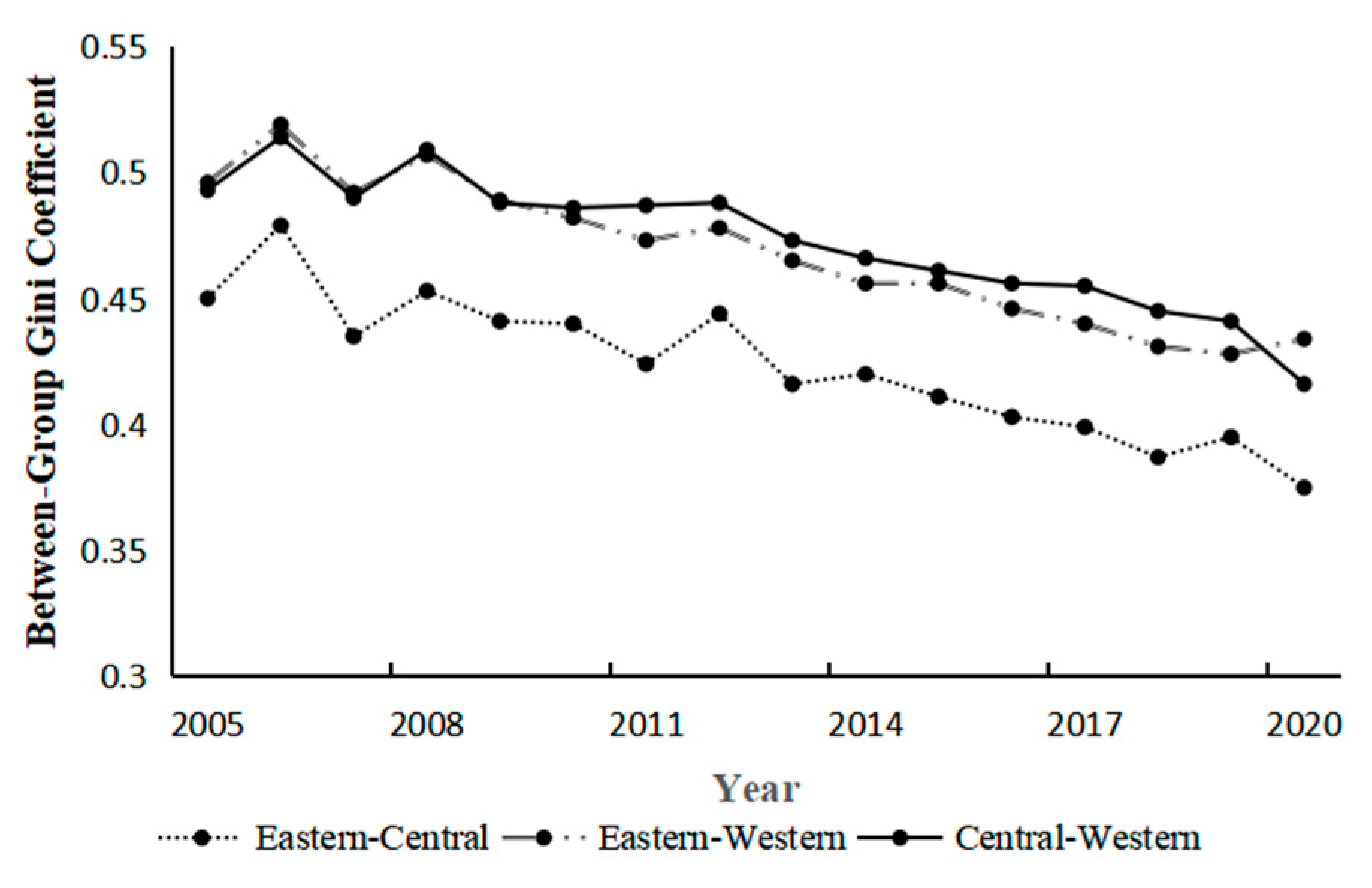
The differences between different regions are shown in Figure 7. Overall, the average differences in GEP levels between the “eastern-central”, “eastern-western”, and “central-western” regions were 0.423, 0.468, and 0.473, respectively, with the average differences involving the western region being larger. From a temporal perspective, from 2005 to 2020, the between-group Gini coefficients showed an overall trend of fluctuating decline, indicating that differences in the ability to realize biophysical values of ecological products among regions are gradually narrowing.

3.2. Spatial Econometric Analysis and Robustness Testing

To enhance the credibility of this study, this paper employs spatial econometric methods to conduct robustness testing on the spatio-temporal characteristics of the accounting results.

3.2.1. Dynamic Evolution of GEP Based on Kernel Density Estimation

In order to provide a more intuitive depiction of the absolute disparities during the sample period, we employ kernel density estimation to illustrate the dynamic progression of absolute differences in GEP across the country. This method generates dynamic distribution plots that reveal the evolutionary pattern of absolute GEP differences and highlight their magnitude and changing features. The detailed formula is as follows (Terrell GR & Scott DW, 1992) [22]:
f j ( y ) = 1 n j h i = 1 n j K ( y j i y h )
where K ( · ) represents the kernel density function, describing the weights of all sample points y j i within the neighborhood y , and h denotes the bandwidth for kernel density estimation. This paper adopts the optimal bandwidth method and uses a Gaussian kernel function to estimate the regional differences, with specific expression as follows:
K ( x ) = 1 2 π e s p ( x 2 2 )
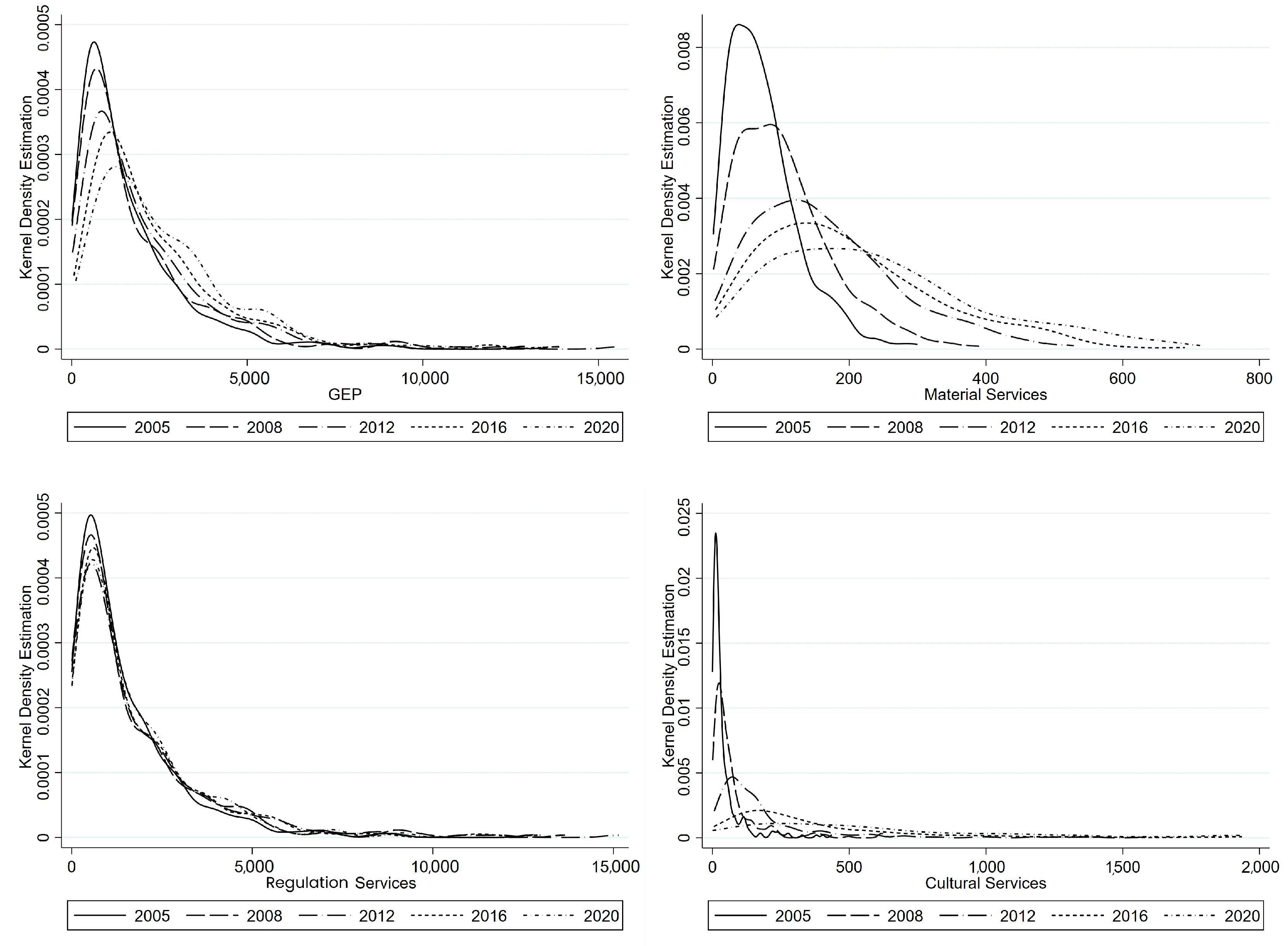
Kernel density estimation reveals the distribution characteristics of sample data across regions, providing detailed descriptions of key attributes such as the distribution location, peak distribution characteristics, distribution spread, and number of peaks of the density curve, thereby capturing the dynamic evolution and changing characteristics of GEP. This paper uses prefecture-level city data while excluding the samples of Beijing, Chongqing, Shanghai, and Tianjin, with results illustrated in Figure 8:
Overall, the kernel density curves for GEP and its three major dimension indicators exhibit a gradual downward trend and an overall rightward shift, reflecting a positive growth trend in GEP levels in most regions of the country and indicating good ecological development. In terms of the peak distribution pattern, the peak height fluctuates with a “gradual decline” during the sample period. Except for regulatory services, the peaks decline and broaden, with the kernel density curves gradually flattening out, indicating a decentralized trend in the distribution of GEP levels across regions.
When examining the three major dimension indicators comprising GEP, the kernel density curves for material product provision and Cultural Services share a similar waveform, with significant rightward shifts and gradually decreasing peak heights, accompanied by shortened right tails. This suggests that the levels of material product provision and Cultural Services in cities have increased annually during the sample period, while the inter-provincial gaps have narrowed year by year. Regulation Services show insignificant changes over time, with only a slight decline in peak height, indicating minimal variation in regulatory service levels among prefecture-level cities during the sample period. This may be attributed to the difficulty in significantly altering the areas of various ecosystems within prefecture-level cities in the short term, resulting in insignificant changes in most regulatory functions.
The results of kernel density estimation are generally consistent with the differences in GEP quantified by the Dagum Gini coefficient.

3.2.2. Spatial Correlation of GEP– Based on Spatial Moran’s I

Entities located in closer geographical proximity demonstrate a stronger level of interconnectedness, indicating the presence of spatial dependence or spatial autocorrelation in the measured values of a specific attribute across various spatial units. This research utilizes Spatial Moran’s I to investigate both the overall and localized spatial autocorrelation of GEP across 273 cities in China, aiming to determine if there exists a spatial relationship in GEP values between these spatial entities.
This paper constructs global and local Moran’s I indices, with the formula for the global Moran’s I index as follows (Anselin L, 1995) [23]:
I = i = 1 n j = 1 n W i j ( X i X ¯ ) ( X j X ¯ ) S 2 i = 1 n j = 1 n W i j
where S 2 = i = 1 n ( X i X ¯ ) 2 / n is the variance, X ¯ = i = 1 n X i / n is the mean, and X i and X j represent the GEP of different prefecture-level cities, respectively; n denotes the number of spatial units (i.e., prefecture-level cities), and W i j = ( W i j ) i * j is the spatial weight matrix reflecting the spatial connections between cities. The values of the global Moran’s I index are in the range of [−1, 1]. When its value approaches 1, it indicates a higher degree of spatial agglomeration of China’s GEP, with spatial positive correlation; when its value approaches −1, it suggests greater spatial variability of China’s GEP, with spatial negative correlation; when its value is close to 0, it implies no spatial correlation of China’s GEP, presenting a random spatial distribution. Simultaneously, this paper introduces two spatial matrices; one is the proximity weight matrix, where the spatial weight matrix takes a value of 1 when a city is geographically adjacent to another, and 0 otherwise. The second is the distance weight matrix, taking the reciprocal of the shortest highway mileage between cities.
Furthermore, to delve deeper into the spatial agglomeration effect of GEP among cities in China and discern potential different spatial correlation forms due to positional differences among spatial units, this paper introduces the local Moran’s I index, with the formula as follows:
= n ( X i X ¯ ) i j W i j ( X j X ¯ ) i = 1 n ( X i X ¯ ) = ( X i X ¯ ) i j W i j ( X j X ¯ ) S 2
The figures for the local Moran’s I index are not confined to the interval between −1 and 1. If the index value notably exceeds 0, it signifies that neighboring spatial units share comparable observed values, indicating a pattern of “high-high” clustering or “low-low” clustering; conversely, if the index value is markedly below 0, it denotes that adjacent spatial units exhibit contrasting observed values, pointing to a pattern of “high-low” clustering or “low-high” clustering.
The results of the global Moran’s I index are shown in Table 4.
As shown in Table 4, the global Moran’s I indices derived from both proximity-based and distance-based spatial weight matrices are statistically significant at the 1% level, confirming strong positive spatial autocorrelation in China’s GEP. This systematic spatial clustering reveals distinct regional patterns; prefecture-level cities with relatively low GEP values tend to cluster adjacent to similarly low-performing areas, while high-GEP cities form contiguous high-value agglomerations. Notably, the global Moran’s I values remain stable across methodologies, in the range of [0.349, 0.481] under the binary contiguity matrix and [0.066, 0.102] for the distance-weighted matrix. Such consistency across spatial weighting schemes underscores the robustness of China’s GEP spatial correlation patterns, reflecting enduring regional interdependencies in ecological–economic dynamics.
The local Moran’s I index calculations cover only the years 2005, 2010, 2015, and 2020, utilizing the distance spatial matrix. The scatter plot results are shown in Figure 9.
The x-axis and y-axis of the Moran’s I scatter plot depict the standardized GEP and its spatial lag (i.e., the weighted mean of surrounding units relative to the observed value), respectively. The inclination of the diagonal line signifies the annual global Moran’s I index value. The first quadrant signifies a high-high positive association, the second quadrant indicates a low-high negative association, the third quadrant denotes a low-low positive association, and the fourth quadrant represents a high-low negative association. Given that all global Moran’s I indices for China’s multi-ecosystem GEP are positive, the primary focus of this study’s observations lies within the first and third quadrants of the scatter plot. Figure 9 illustrates that, over the years, the majority of provinces are situated within these key observation zones, strongly indicating the enduring significance of the positive spatial correlation in China’s GEP.
While the global Moran’s I indicates positive spatial autocorrelation (Figure 9), the scatter plot reveals heterogeneous local dynamics. A majority of prefectures fall into the high-high (HH) and low-low (LL) quadrants, suggesting two dominant clusters:
High-value clusters: Likely concentrated in southwestern China (e.g., Yunnan, Sichuan) where forest ecosystems and biodiversity conservation policies (e.g., the Grain-to-Green Program) enhance GEP synergies [24].
Low-value clusters: Predominant in arid northwestern regions (e.g., Ningxia, Gansu) constrained by water scarcity and fragile ecosystems [25].
Notably, outliers in the high-low (HL) quadrant (e.g., Shanghai, Shenzhen) reflect urban centers with high GEP values contrasting neighboring low-value areas, likely due to intensive ecological investments offsetting urbanization pressures [26]. These patterns align with regional socio-ecological gradients and call for spatially targeted governance.

3.3. Driving Mechanisms

The uncoordinated ecological development and insufficient realization of GEP we have observed are caused by three interrelated driving mechanisms tied to China’s unique ecological–economic transition.

3.3.1. Resource Endowment Versus Utilization Efficiency

Western China exhibits a paradoxical situation where, despite accounting for a substantial 46% of the national Gross Ecosystem Product (GEP) volume, its per-unit-area GEP value is merely 72% of the national average, reflecting a phenomenon akin to the “resource curse” [27,28]. Although this region is blessed with extensive forests and grasslands (as detailed in Table 2), the scarcity of technological inputs and the over-reliance on low-value ecosystems, such as degraded grasslands, impede the full realization of ecosystem service values [29]. In stark contrast, eastern regions capitalize on their relatively compact ecosystems, like urban wetlands, through intensive management practices. As a result, they achieve a higher GEP density, reaching 128% of the national average (as illustrated in Figure 4). This regional disparity aligns with global trends, where resource-abundant regions often struggle to transform their natural capital into improved welfare outcomes in the absence of innovative approaches [30].

3.3.2. Dual Constraints of Natural Thresholds and Market Failures

The fact that the Gross Ecosystem Product (GEP) is growing at a notably slower pace of 3.18% annually, in stark contrast to the GDP’s robust 12.05% growth rate, underscores the path dependency inherent in traditional growth models [31]. Regulation services, which account for a substantial 65% of the total GEP, are unfortunately caught in a vicious cycle of “high-input, low-output”, as they are only expanding at a sluggish 0.88% per year (as shown in Figure 3). This predicament stems from two primary factors. Firstly, there are natural thresholds at play. After decades of afforestation efforts, for instance, between 2005 and 2020, although the forest area increased by less than 2%, the growth in net primary productivity (NPP), a key indicator, stagnated. This indicates that water retention and carbon sequestration, crucial components of regulation services, are now facing diminishing returns. Secondly, market failures exacerbate the issue. While cultural services in eastern cities have experienced rapid growth of 18.63% annually, largely driven by tourism (as detailed in Table 1), western regions are left behind due to a lack of necessary infrastructure to monetize their comparable natural and cultural assets [32].

3.3.3. Policy Implementation Gaps

Spatial disparities, indicated by a Dagum Gini coefficient of 0.452, highlight uneven governance capacities across regions. Western provinces face high internal inequality because of their fragmented ecosystems and inconsistent policy implementation (as shown in Figure 6). For instance, although “ecological redline” policies safeguard forests, inadequate compensation mechanisms—with less than 30% of western cities meeting cross-provincial GEP payment targets—discourage local governments from taking good care of ecosystems [33]. In contrast, eastern regions incorporate GEP into urban planning via carbon markets and eco-tourism zoning, leading to better coordination and a 1.04% annual decline in their intra-regional Gini coefficient. These dynamics form a self-perpetuating cycle; resource-rich regions prioritize short-term GDP growth over ecosystem optimization, and the resulting slow value realization of ecosystems further widens regional imbalances [34]. To break this cycle, it is crucial to tackle both physical limitations, like ecosystem restoration thresholds, and institutional obstacles, such as mismatched fiscal incentives.

4. Discussion

4.1. Conclusion

This study provides the first national-scale assessment of China’s Gross Ecosystem Product (GEP) from 2005 to 2020, advancing three key findings that both align with and challenge prior research. First, while our observed 57.7% GEP growth corroborates the literature [5], its lag behind GDP (3.18% vs. 12.05% annually) echoes global debates on the undervaluation of ecosystem services in economic transitions [1]. Second, the stagnation of regulation services—despite their dominance (CNY 48.72 trillion in 2020)—contrasts with studies emphasizing cultural services as the fastest-growing component in developed regions [6], highlighting China’s unique challenge in balancing natural capital preservation with urbanization pressures. Third, our spatial decomposition of disparities (Dagum Gini = 0.452) extends earlier provincial analyses [20], revealing that western China’s high GEP volume but low efficiency mirrors patterns in Brazil’s Amazonian states, where vast ecosystems struggle to translate biophysical abundance into localized welfare [2].

4.2. Study Limitations

This study’s dependence on provincial-scale economic datasets introduces limitations in detecting localized ecological variations, particularly within complex systems like Guangxi’s karst landscapes. While our methodology achieves county-level resolution for quantifying regulatory services, a critical discrepancy arises between county-level ecological measurements and provincial-scale Dagum Gini coefficient analyses. This spatial mismatch is particularly evident in megacity systems such as Chengdu, where urban cores exhibit GEP intensities 5.8 times higher than adjacent mountainous counties—a disparity obscured by macro-scale analyses that inadequately address intra-regional ecological–economic gradients. Methodologically, the geographic scope diverges from international standards like the EU’s Ecosystem Mapping Project, which employs 500 m grids for enhanced precision. To resolve these multi-scale challenges, future studies can use a nested monitoring system integrating hyperspectral remote sensing with IoT-based sensor arrays. Such an approach would align provincial administrative boundaries with ecologically sensitive micro-zones while adhering to IPBES assessment protocols.
Furthermore, the analysis focuses predominantly on terrestrial ecosystems, with limited incorporation of marine systems that constitute critical coastal ecological assets. This exclusion may compromise GEP comprehensiveness in coastal provinces, where blue carbon sequestration functions (e.g., Fujian’s mangrove ecosystems) remain underrepresented. Preliminary estimates suggest marine contributions could enhance current GEP valuations by 12–15% in these regions. Future studies should extend this framework through marine ecosystem service accounting, incorporating satellite-derived bathymetry and coastal habitat mapping to strengthen spatial integrity and system completeness.

4.3. Suggestions

By integrating ecosystem services theory with Dagum Gini decomposition, we propose a three-dimensional framework (resource endowment–capacity–governance) that addresses limitations in existing governance models. Our framework synergizes market mechanisms (e.g., cross-provincial GEP quotas) with adaptive governance (e.g., ecological redlines), offering a scalable solution for emerging economies. For instance, applying this to the Mekong River Basin could resolve transboundary conflicts over hydropower versus sediment retention—a challenge parallel to China’s Yangtze River governance [25]. Translating this framework into action requires multi-level governance for emerging economies facing similar trade-offs, such as Brazil’s Amazon conservation challenges and transboundary ecological compensation mechanisms in the Mekong River Basin.
Looking ahead, we put forward several policy suggestions, as follows.
First is National-Level Strategic Interventions. Under the leadership of the National Development and Reform Commission (NDRC) and Ministry of Ecology and Environment (MEE), China should formalize an Integrated Ecological Compensation System (IECS) to address upstream–downstream ecological–economic disparities and mitigate development pressures in ecologically fragile western regions. Key initiatives should include (1) establishing a Central Ecological Fund (CEF); (2) launching Special Ecological Treasury Bonds to finance national park networks and cross-basin ecological security projects; (3) expanding the National Protected Area system with strict non-conversion clauses.
Second is Provincial-Level Collaborative Governance. Provincial governments should leverage market-driven mechanisms and institutional innovations to accelerate inter-regional synergies, thereby addressing the ecological resource depletion caused by excessive emphasis on economic growth at the expense of ecological endowments during provincial development. Key initiatives should include (1) implementing Watershed GEP Quota Trading (e.g., downstream provinces purchase upstream water purification credits); (2) creating Cross-Provincial GEP Exchange Platforms (e.g., enable Yunnan to sell forest carbon sink futures).
Third is Micro-Level Behavioral Incentives. Local governments should adopt targeted incentive mechanisms and participatory governance frameworks to empower individuals and enterprises with decision-making authority over ecological management, thereby enhancing their ecological accountability. Key initiatives include (1) rolling out Personal Ecological Accounts (e.g., award residents digital credits for low-carbon behaviors); (2) enforcing Corporate GEP Accountability Standards; and (3) initiating County-Level Ecological Performance Tournaments.
Finally, the international scalability of China’s GEP-driven governance model presents a replicable blueprint for emerging economies navigating ecological–development trade-offs. Leveraging China’s spatially heterogeneous GEP patterns—characterized by the western high-volume/low-efficiency paradox—and its proven three-tier governance framework, these economies can adapt tailored mechanisms. (1) Federal states (e.g., Brazil) could adopt biome-specific fiscal transfers—modeled on China’s Central Ecological Fund—to compensate conservation regions (e.g., Amazon states) via constitutional revenue sharing, addressing core–periphery GEP disparities akin to China’s west–east imbalance. (2) Transboundary watersheds (e.g., Mekong) may institute GEP credit trading to monetize upstream conservation (e.g., Vietnamese agribusinesses buying Cambodian floodplain sediment retention credits), replicating China’s cross-regional value flow optimization. (3) Community-led regions (e.g., Kenya’s pastoralist areas) could deploy blockchain-verified indigenous ecological accounts that integrate traditional practices with behavioral incentives, mirroring China’s marginal ecosystem governance.
In conclusion, this study advances the discourse on China’s ecological transition by systematically evaluating the GEP framework and its regional development disparities. By integrating quantitative assessments of ecological–economic trade-offs, it provides a policy-relevant insights for harmonizing rapid industrialization with ecosystem conservation in emerging economies, and provides a scalable analytical framework for cross-border ecological asset management and sustainable development governance. The findings will be a critical reference for policymakers, researchers, and international bodies addressing the ecological–industrial nexus in developing contexts.

Author Contributions

Conceptualization, X.Y. and H.Y.; methodology, X.Y. and Y.S.; software, X.Y.; validation, X.Y., H.Y. and Y.S.; formal analysis, H.Y.; investigation, Y.S.; resources, Y.S.; data curation, X.Y.; writing—original draft preparation, X.Y.; writing—review and editing, H.Y.; visualization, Y.S.; supervision, Y.S.; project administration, X.Y.; funding acquisition, H.Y. All authors have read and agreed to the published version of the manuscript.

Funding

This work was supported by the Major Projects of National Social Science Fund of China [22ZDA108]; Key Project of Cultivating Representative Achievements of Graduate Students in Southwestern University of Finance and Economics [JGS2024017].

Institutional Review Board Statement

Not applicable.

Informed Consent Statement

Not applicable.

Data Availability Statement

The data presented in this study are available on request from the corresponding author.

Conflicts of Interest

The authors declare no conflicts of interest.

Appendix A

Table A1. Definition of indicators of GEP.
IndicatorIndicator Description
Material Product Supply  Ecosystems in China’s districts and counties provide a wide range of material products including agricultural, forestry, animal husbandry, fishery products, and ecological energy.
  The biophysical value of these products are derived from the statistical yearbooks of respective districts and counties.
  The monetary value of material services is determined using the market value method.
Water Conservation  Water conservation services refer to the ecosystem’s ability to intercept, store, and infiltrate precipitation, thereby enhancing soil moisture, regulating storm runoff, replenishing groundwater, and increasing the availability of water resources.
  The biophysical value of water conservation is calculated using the Integrated Valuation of Ecosystem Services and Trade-offs model (InVEST model), specifically its Water Yield module.
  The monetary value of water conservation, primarily manifested in its economic benefit for water storage and retention, is assessed using the shadow engineering approach.
Soil Conservation  Soil conservation involves protecting the soil from erosion, increasing soil resilience, and reducing soil loss through various ecosystem components such as forest canopies, litter, and root systems.
  The biophysical value of soil conservation is calculated using the InVEST model’s Soil Retention module, which incorporates elevation data, rainfall erosivity factor, soil erodibility factor, land use data, biophysical tables, parameters, and watershed boundaries to generate raster data on potential and actual soil erosion for various ecosystems nationwide.
  The monetary value of soil conservation is assessed using the replacement cost method, which considers the reduction in non-point source pollution and sediment deposition.
Sand Storm Prevention  Sand storm prevention refer to the ecosystem’s ability to mitigate soil loss and sandstorm hazards caused by strong winds.
  The physical quantity of windbreak and sand fixation is calculated using the Revised Wind Erosion Equation (RWEQ).
  The value of sand storm prevention is assessed using the restoration cost method, which considers the cost of rehabilitating degraded sandy land or restoring vegetation.
Flood Regulation and Storage  Flood regulation and storage refers to the natural ecosystem’s ability to absorb large amounts of precipitation and transit water, store flood peak water volume, reduce and delay flood peaks, thereby mitigating the threats and losses caused by flood peaks during the flood season.
  This study follows the approach of Wang Liyan et al. (2017) to examine the function of lakes and marshes in regulating and storing floodwater to mitigate flood threats [20]. The physical quantity of flood regulation is calculated based on the area of various ecosystems, using the following formula:
  This study employs the shadow engineering method, using the construction cost of reservoirs to calculate the monetary value of flood regulation regulation and storage by natural ecosystems:
Air Purification  Air purification refers to the ecosystem’s ability to absorb, filter, block, and decompose air pollutants (such as SO2, NOx, particulate matter, etc.), thereby improving the atmospheric environment.
  In this study, only the ecosystem’s ability to absorb SO2, NOx, and dust are considered to calculate the biophysical value of air purification [7,35,36,37].
  This study uses the replacement cost method to calculate the value of air purification by considering the cost of industrial air pollutant treatment [38,39].
Water Purification  Water purification refers to the ability of aquatic ecosystems such as lakes, rivers, and marshes to adsorb, degrade, and transform water pollutants, thereby purifying the aquatic environment.
  In this study, the purification capacity of ecosystem for COD, total nitrogen and total phosphorus is considered to calculate the biophysical value of water purification [40,41].
  Similar to air purification, this study uses the replacement cost method to calculate the monetary value of water purification by considering the cost of water pollutant treatment.
Carbon Sequestration  Carbon sequestration refers to the ecosystem’s ability to absorb atmospheric CO2, synthesize organic matter, and store carbon in plants or soils.
  This study calculates the biophysical value of terrestrial ecosystem carbon sequestration using the Net Ecosystem Productivity (NEP) method [39,42].
  The monetary value of ecosystem carbon sequestration can be calculated using the market value method and the carbon market trading price.
Oxygen Provision  The oxygen release function of ecosystems refers to the plants’ ability to release oxygen during photosynthesis, thereby maintaining atmospheric oxygen stability and improving the human living environment.
  This study calculates the biophysical value of oxygen release capacity using the NEP method based on the chemical equation of photosynthesis:
  The monetary value of ecosystem oxygen provision is calculated using the market value method and the industrial oxygen production price:
Climate Regulation  Climate regulation services refer to the ecosystem’s ability to absorb solar energy through vegetation transpiration and water surface evaporation, thereby lowering temperature, increasing air humidity, and improving human living comfort.
  This study uses the biophysical value of total energy consumed by ecosystem transpiration and evaporation as the physical quantity of climate regulation.
  This study employs the replacement cost method, using the electricity consumption required for artificial temperature and humidity regulation to calculate the monetary value of ecosystem climate regulation.
Tourism and Landscapes  Ecosystems in various districts and counties in China provide humans with the functions of leisure tourism and landscape appreciation. The physical quantity and value of these services are derived from the statistical yearbook data of each district and county. The monetary value of cultural services is calculated using the method of monetary market value and tourism revenue.
Table A2. Measurement method for GEP.
Function Secondary
Indicators
Indicator
Formula
Formula
Description
Material Product SupplyAgricultural;
Forestry;
Animal Husbandry;
Fishery;
Other Product;
Ecological Energy
V p = i = 1 n E i P i V p represents the biophysical value
E i represents the output (kg) of the i-th product
P i denotes the unit price (CNY/kg) of the i-th product.
Regulation ServicesWater Conservation V w r = Q w r C w e V w r is the monetary value of water conservation (CNY/a)
Q w r represents the biophysical value within the assessment area (m3/a)
C w e denotes the construction and maintenance cost per unit storage capacity of a reservoir (CNY/m3).
Soil Conservation V w r = Q w r C w e
Q s r = R K L S U S L E
R K L S = R K L S
U S L E = R K L S P C
V s r = V s d + V d b d
V s d = λ Q s r ρ c
V d b d = i = 1 n Q s r C i P i
Q s r is the biophysical value of soil conservation (t/a)
R represents the rainfall erosivity factor
K denotes the soil erodibility factor
L and S are the slope length and steepness factors (dimensionless)
C and P are the vegetation cover and management factor and soil conservation practice factor (dimensionless)
V s r is the total monetary value of soil conservation (CNY/a)
V s d represents the monetary value of reducing sediment deposition (CNY/a)
V d b d denotes the monetary value of reducing non-point source pollution (CNY/a).
Sand Storm Prevention Q s f = 0.1699
( W F E F S C F K ) 1.3711
1 C 1.3711
V s f = Q s f ρ h C
Q s f is the biophysical value of sand storm prevention (t/a)
WF represents the climatic factor (kg/m)
EF denotes the soil erodibility factor, SCF is the soil crusting factor
K is the surface roughness factor, C is the vegetation cover factor.
V s f is the monetary value of sand storm prevention (CNY/a)
ρ denotes the soil bulk density (t/m3)
h is the thickness of sand covering the soil (m)
C represents the cost of sand control engineering per unit area (CNY/m2).
Flood Regulation and Storage C f m = C l c + C m c
C m c = S 1 h ρ F E 100 ρ w
+ S 2 H 10 2
V f m = C f m C w e
C f m is the biophysical value of flood regulation and storage (m3)
C l c is the flood regulation capacity of lakes (m3)
C m c is the flood regulation capacity of marshes (m3).
S 1 is the total marsh area (km2)
h is the soil water storage depth in marsh wetlands
ρ is the soil bulk density of marsh wetlands (g/cm3)
ρ w is the density of water (g/cm3)
F is the soil saturated water content of marsh wetlands (dimensionless)
E is the natural water content of marsh wetlands before flooding (dimensionless).
S 2 is the total marsh area (km2)
H is the surface water storage height in marsh wetlands
V f m is the monetary value of ecosystem flood regulation (CNY)
C w e is the construction cost per unit storage capacity of the reservoir
Air Purification Q a p = i = 1 n j = 1 m Q i j A i
V a = j = 1 m Q a p j C j
Q a p is the biophysical value of air purification capacity of the ecosystem (kg)
Q i j is the unit area purification capacity of the j-th air pollutant by the i-th type of ecosystem (kg/km2), i represents the ecosystem type (forest, shrubland, grassland; dimensionless)
Aᵢ is the area of the i-th type of ecosystem (km2), and j represents the type of air pollutant (SO2, NOx, dust) (dimensionless).
V a is the monetary value of air purification by the ecosystem (CNY)
C j is the treatment cost of the j-th air pollutant (CNY/t) [41,43,44].
Water Purification Q w p = i = 1 n k = 1 m P i k A i
V w = g = 1 m Q w p g C g
Q w p is the biophysical value of water purification capacity (kg)
V w is the monetary value of water purification by the ecosystem (CNY/a)
C g is the treatment cost of the j-th water pollutant (CNY/t)
Carbon Sequestration Q t c o 2 = ( M c o 2 M c ) N E P
V c f = Q C O 2 C C
Q t c o 2 is the biophysical value of carbon sequestration capacity of the terrestrial ecosystem (t)
NEP is calculated based on the NPP and the conversion coefficient provided in the guidelines.
V c f is monetary the value of ecosystem carbon sequestration (CNY)
C C is the carbon price
Oxygen Provision Q o p = ( M O 2 M C O 2 ) Q t c o 2
V o p = Q o p C o
Q o p is the biophysical value of oxygen release capacity of the ecosystem (t·O2)
Q t c o 2 is the carbon sequestration capacity of the terrestrial ecosystem (t·CO2)
V o p is the monetary value of ecosystem oxygen provision (CNY/a)
C o is the industrial oxygen production price
Climate Regulation E t t = i = 1 3 E P P i S i D 3600 r 10 6
+ E w q 10 3 / ( 3600 )
+ E w y
V t t = E t t P e
E t t is the biophysical value of energy consumed by ecosystem transpiration and evaporation (kW·h)
E p t is the energy consumed by ecosystem vegetation transpiration (kW·h)
E w e is the energy consumed by wetland ecosystem evaporation (kW·h).
V t t is the monetary value of ecosystem climate regulation (CNY/a)
P e is the local electricity price (CNY/kW·h)
Cultural ServicesTourism and Landscapes V r = V C C + V C S V r is the monetary value of cultural services (CNY)
V C C is the monetary value of tourism (CNY)
V C S is the monetary value of landscapes (CNY)
Table A3. Data and database.
Secondary
Indicator
DataDatabase (Data Source)
Product SupplyValue-added China County Statistical Yearbook (County Bureau of Statistics)
Water ConservationPrecipitationMonthly Precipitation and Evapotranspiration Data
(National Geographical System Science Data Center)
Evapotranspiration
Root depthBedrock Depth Data [45,46,47]
Plant-available
water content
World Soil Database (National Tibetan Plateau Data Center)
Land useCLCD Data
(School of Remote Sensing and Information Engineering, Wuhan University)
Watershed boundaryElevation Data (Geospatial Data Cloud)
Soil ConservationSlope data
Rainfall erosivity factorAnnual Precipitation Data (National Geographical System Science Data Center)
Soil erodibility factorWorld Soil Database (National Tibetan Plateau Data Center)
Land useCLCD Data
(School of Remote Sensing and Information Engineering, Wuhan University)
Watershed boundaryElevation Data (Geospatial Data Cloud)
Sand Storm PreventionWind force factorDaily Wind Speed Data, Precipitation, Evapotranspiration Data
(National Geographical System Science Data Center)
Soil moisture
Snow cover factorChina’s Long Time Series Snow Depth Dataset
(National Tibetan Plateau Data Center)
Soil erodibility factorWorld Soil Database (National Tibetan Plateau Data Center)
Soil crusting factor
Vegetation cover factorChina’s Annual Vegetation (NDVI) Data
(Chinese Academy of Sciences Resource and Environment Science Data Platform)
Surface roughness factorElevation Data (Geospatial Data Cloud)
Flood Regulation and StorageLake areaCLCD Data
(School of Remote Sensing and Information Engineering, Wuhan University)
Lake regionChina Lake Records (The Technical Guideline on Gross Ecosystem Product)
Air purificationForest, shrubland, and grassland areaCLCD Data
(School of Remote Sensing and Information Engineering, Wuhan University)
Absorption capacity of atmospheric pollutantsLiterature [7,35,36,37,47,48,49]
Water PurificationWetland areaCLCD Data
(School of Remote Sensing and Information Engineering, Wuhan University)
Absorption capacity of water pollutantsLiterature [38,42]
Carbon SequestrationNet ecosystem productivity (NEP)Net Primary Productivity (NPP) (Google Earth Engine platform)
NPP conversion factorConversion Factors of Provinces and Cities
(The Technical Guideline on Gross Ecosystem Product)
Oxygen ProvisionNEPNet primary Productivity (NPP) (Google Earth Engine platform)
Climate RegulationForest, shrubland, and grassland areaCLCD Data
(School of Remote Sensing and Information Engineering, Wuhan University)
Number of days with max daily temperature above 26 °CDaily Temperature Data and Monthly Evapotranspiration Data
(National Geographical System Science Data Center)
Water surface evaporationCLCD Data
(School of Remote Sensing and Information Engineering, Wuhan University)
Tourism and LandscapesTourism revenueChina County Statistical Yearbook (County Bureau of Statistics)
Figure A1. Spatial distribution of average GEP and regulation services in China (the units of all monetary value are in hundred billion yuan).
Sustainability 17 04451 g0a1

References

  1. Costanza, R.; d’Arge, R.; de Groot, R.; Farber, S.; Grasso, M.; Hannon, B.; Limburg, K.; Naeem, S.; O’Neill, R.V.; Paruelo, J.; et al. The Value of the World’s Ecosystem Services and Natural Capital. Nature 1997, 387, 253–260. [Google Scholar] [CrossRef]
  2. Joshi, A.P.; Joshi, S.; Sudhanshu, R.K.; Pant, D.; Rai, S.; Rawat, A.; Purohit, H. Deciphering Uttarakhand’s human efforts towards the ecology through Gross Environment Product (GEP) calculations. Environ. Sustain. Indic. 2025, 25, 100578. [Google Scholar] [CrossRef]
  3. Peng, T.; Wu, W. Green GDP Accounting: Further Research and Discussion in the Context of Low-carbon Development. China Popul. Resour. Environ. 2010, 20, 81–86. [Google Scholar]
  4. Wang, N.; Liu, J.; Wu, D.; Gao, S.; Wang, R. Regional Eco-compensation based on Ecosystem Service Assessment: A Case Study of Shandong Province. Acta Ecol. Sin. 2010, 30, 6646–6653. [Google Scholar]
  5. Ma, G.; Yu, F.; Wang, J.; Zhou, X.; Yuan, J.; Mou, X.; Zhou, Y.; Yang, W.; Peng, F. Measuring Gross Ecosystem Product (GEP) of 2015 for Terrestrial Ecosystems in China. China Environ. Sci. 2017, 37, 1474–1482. [Google Scholar]
  6. Wang, J.; Ma, G.; Yu, F.; Peng, F.; Yang, W.; Zhou, X.; Zhou, Y.; Zhao, X. Study on China’s Gross Economic-ecological Product Accounting in 2015. China Popul. Resour. Environ. 2018, 28, 1–7. [Google Scholar]
  7. Wu, Y.; Kang, W.; Guo, Q.; Wang, W. Functional Value of Absorption and Purgation to Atmospheric Pollutants of Urban Forest in Guangzhou. Sci. Silvae Sin. 2009, 45, 42–48. [Google Scholar]
  8. Dagum, C. Decomposition and interpretation of Gini and the generalized entropy inequality measures. Statistica 1997, 57, 295–308. [Google Scholar]
  9. Ma, T.; Liu, Y.; Yang, M. Spatial-temporal heterogeneity for commercial building carbon emissions in China: Based the Dagum Gini coefficient. Sustainability 2022, 14, 5243. [Google Scholar] [CrossRef]
  10. Bosch, J.M.; Hewlett, J.D. A Review of Catchment Experiments to Determine the Effect of Vegetation Changes on Water Yield and Evapotranspiration. J. Hydrol. 1982, 55, 3–23. [Google Scholar] [CrossRef]
  11. Zhou, G.; Wei, X.; Chen, X.; Zhou, P.; Liu, X.; Xiao, Y.; Sun, G.; Scott, D.F.; Zhou, S.; Han, L.; et al. Global Pattern for the Effect of Climate and Land Cover on Water Yield. Nat. Commun. 2015, 6, 5918. [Google Scholar] [CrossRef] [PubMed]
  12. Stuerck, J.; Poortinga, A.; Verburg, P.H. Mapping Ecosystem Services: The Supply and Demand of Flood Regulation Services in Europe. Ecol. Indic. 2014, 38, 198–211. [Google Scholar] [CrossRef]
  13. Nedkov, S.; Burkhard, B. Flood Regulating Ecosystem Services—Mapping Supply and Demand, in the Etropole Municipality, Bulgaria. Ecol. Indic. 2012, 21, 67–79. [Google Scholar] [CrossRef]
  14. Bennett, H.H. Soil Conservation, 1st ed.; McGraw-Hill Book Company: New York, NY, USA, 1939; pp. 1–993. [Google Scholar]
  15. Lal, R. Soil Conservation and Ecosystem Services. Int. Soil Water Conserv. Res. 2014, 2, 36–47. [Google Scholar] [CrossRef]
  16. Huang, J.; Wang, H.; Dai, Q.; Han, D. Analysis of NDVI Data for Crop Identification and Yield Estimation. IEEE J. Sel. Top. Appl. Earth Obs. Remote Sens. 2017, 7, 4374–4384. [Google Scholar] [CrossRef]
  17. Huang, J.; Wang, X.; Li, X.; Tian, H.; Pan, Z. Remotely Sensed Rice Yield Prediction Using Multi-Temporal NDVI Data Derived from NOAA’s-AVHRR. PLoS ONE 2013, 8, e70816. [Google Scholar] [CrossRef]
  18. Cramer, W.; Kicklighter, D.W.; Bondeau, A.; Iii, B.M.; Churkina, G.; Nemry, B.; Ruimy, A.; Schloss, A.L.; ThE Participants OF ThE Potsdam NpP Model Intercomparison. Comparing Global Models of Terrestrial Net Primary Productivity (NPP): Overview and Key results. Glob. Change Biol. 1999, 5 (Suppl. S1), iii–iv. [Google Scholar] [CrossRef]
  19. Dong, T.; Zhang, L.; Xiao, Y.; Zheng, H.; Huang, B.; Ouyang, Z. Assessment of Ecological Assets and Gross Ecosystem Product Value in Ordos City. Acta Ecologica Sinica 2019, 39, 3062–3074. [Google Scholar]
  20. Wang, L.; Yi, X.; Zhiyun, O.; Qin, W.; Wenjing, B.; Jian, Z.; Ling, R. Gross Ecosystem Product Accounting in the National Key Ecological Function Area:an Example of Arxan. China Popul. Resour. Environ. 2017, 27, 146–154. [Google Scholar]
  21. Cai, Q.; Fang, D.; Chen, B. Social vulnerability assessment for air pollution in China. Environ. Impact Assess. Rev. 2025, 114, 107925. [Google Scholar] [CrossRef]
  22. Terrell, G.R.; Scott, D.W. Variable kernel density estimation. Ann. Stat. 1992, 20, 1236–1265. [Google Scholar] [CrossRef]
  23. Anselin, L. Local indicators of spatial association—LISA. Geogr. Anal. 1995, 27, 93–115. [Google Scholar] [CrossRef]
  24. Liu, J.; Li, S.; Ouyang, Z.; Tam, C.; Chen, X. Ecological and socioeconomic effects of China’s policies for ecosystem services. Proc. Natl. Acad. Sci. USA 2008, 105, 9477–9482. [Google Scholar] [CrossRef]
  25. Fu, B.; Wang, S.; Liu, Y.; Liu, J.; Liang, W.; Miao, C. Hydrogeomorphic ecosystem responses to natural and anthropogenic changes in the Loess Plateau of China. Annu. Rev. Earth Planet. Sci. 2017, 45, 223–243. [Google Scholar] [CrossRef]
  26. Zhu, Z.; Ren, J.; Liu, X. Green infrastructure provision for environmental justice: Application of the equity index in Guangzhou, China. Urban For. Urban Green. 2019, 46, 126443. [Google Scholar] [CrossRef]
  27. Auty, R. Sustaining Development in Mineral Economies: The Resource Curse Thesis, 3rd ed.; Routledge: London, UK, 2002; pp. 1–288. [Google Scholar]
  28. Sachs, J.D.; Warner, A.M. The curse of natural resources. Eur. Econ. Rev. 2001, 45, 827–838. [Google Scholar] [CrossRef]
  29. Liu, J.; Raven, P.H. China’s environmental challenges and implications for the world. Crit. Rev. Environ. Sci. Technol. 2010, 40, 823–851. [Google Scholar] [CrossRef]
  30. Bryan, B.A.; Gao, L.; Ye, Y.; Sun, X.; Connor, J.D.; Crossman, N.D.; Stafford-Smith, M.; Wu, J.; He, C.; Yu, D.; et al. China’s response to a national land-system sustainability emergency. Nature 2018, 559, 193–204. [Google Scholar] [CrossRef]
  31. Rockström, J.; Steffen, W.; Noone, K.; Persson, Å.; Chapin, F.S., III; Lambin, E.; Lenton, T.M.; Scheffer, M.; Folke, C.; Schellnhuber, H.J.; et al. Planetary boundaries: Exploring the safe operating space for humanity. Ecol. Soc. 2009, 14, 32. [Google Scholar] [CrossRef]
  32. Daily, G.C.; Polasky, S.; Goldstein, J.; Kareiva, P.M.; Mooney, H.A.; Pejchar, L.; Ricketts, T.H.; Salzman, J.; Shallenberger, R. Ecosystem services in decision making: Time to deliver. Front. Ecol. Environ. 2009, 7, 21–28. [Google Scholar] [CrossRef]
  33. Liu, Y.; Li, Y. Revitalize the world’s countryside. Nature 2017, 548, 275–277. [Google Scholar] [CrossRef] [PubMed]
  34. Lo, K. Ecological civilization, authoritarian environmentalism, and the eco-politics of extractive governance in China. Extr. Ind. Soc. 2020, 7, 1029–1035. [Google Scholar] [CrossRef]
  35. Han, S.Y.; Tian, D.L.; Yan, W.D.; Liang, X.C.; Wang, G.J.; Zhu, F. Evaluation of Eco-service Functions of Major Forest Types in Hunan Province. J. Cent. South Univ. For. Technol. 2009, 29, 6–13. [Google Scholar]
  36. Zhao, Y.; Li, S.; Yan, Z. The Effect of Greenland on Absorbed Dust and Its Assessment Method. J. Huazhong Agric. Univ. 2002, 6, 582–586. [Google Scholar]
  37. Jia, J.; Luo, W.; Du, T.; Li, Z.; Lu, Y. Valuation of Changes of Ecosystem Services of Tai Lake in Recent 10 years. Acta Ecol. Sin. 2015, 35, 2255–2264. [Google Scholar]
  38. Zhang, B.; Gao, J.; Xie, G.; Wang, Y. Preliminary Evaluation of Air Temperature Reduction of Urban Green Spaces in Beijing. Acta Ecol. Sin. 2012, 32, 7698–7705. [Google Scholar] [CrossRef]
  39. Li, G.; Zhao, W.; Wei, Y.; Fang, X.; Gao, B.; Dai, L. Evaluation on the Influence of Natural Forest Protection Program on Forest Ecosystem Service Function in Changbai Mountain. Acta Ecol. Sin. 2015, 35, 984–992. [Google Scholar]
  40. Zhou, Z.; Li, J.; Feng, X. The Value of Fixing Carbon and Releasing Oxygen in the Guanzhong-Tianshui Economic Region using GIS. Acta Ecol. Sin. 2013, 33, 2907–2918. [Google Scholar] [CrossRef]
  41. Baskent, E.Z.; Borges, J.G.; Kašpar, J.; Tahri, M. A design for addressing multiple ecosystem services in forest management planning. Forests 2020, 11, 1108. [Google Scholar] [CrossRef]
  42. Yan, F.; Shangguan, W.; Zhang, J.; Hu, B. Depth-to-bedrock Map of China at a Spatial Resolution of 100 Meters. Sci. Data 2020, 7, 2. [Google Scholar] [CrossRef]
  43. Suding, K.; Spotswood, E.; Chapple, D.; Beller, E.; Gross, K. Ecological dynamics and ecological restoration. In Foundations of Restoration Ecology; Island Press: Washington, DC, USA, 2016; pp. 27–56. [Google Scholar]
  44. Jin, X.; Fang, D.; Chen, B.; Wang, H. Multiobjective layout optimization for low impact development considering its ecosystem services. Resour. Conserv. Recycl. 2024, 209, 107794. [Google Scholar] [CrossRef]
  45. Li, Q.; Sun, G. Study on Annual Changes and Synchronousness of Atmosphere Pollution Reduction by Woodland and Grassland in Xi’an. Syst. Sci. Compr. Stud. Agric. 2008, 1, 73–77. [Google Scholar]
  46. Cai, Q.; Fang, D.; Chen, B. Ecological network analysis for urban physical-virtual water cycle: A case study of Beijing. Ecol. Model. 2025, 501, 110972. [Google Scholar] [CrossRef]
  47. Jin, X.; Jiang, W.; Fang, D.; Wang, S.; Chen, B. Evaluation and driving force analysis of the water-energy-carbon nexus in agricultural trade for RCEP countries. Appl. Energy 2024, 353, 122143. [Google Scholar] [CrossRef]
  48. Yuan, Z.; Tian, D.; Yuan, H. Research on SO2 Cleansing Ability of the Air of Forest Biology System and Sabsorbed Potential. Hunan For. Sci. Technol. 2005, 1, 1–4. [Google Scholar]
  49. Ma, X.; Sun, G.; Ren, Z. The Values of Vegetation Purified Air and Its Measure in Xin’an City. J. Arid. Land Resour. Environ. 2002, 4, 83–86. [Google Scholar]
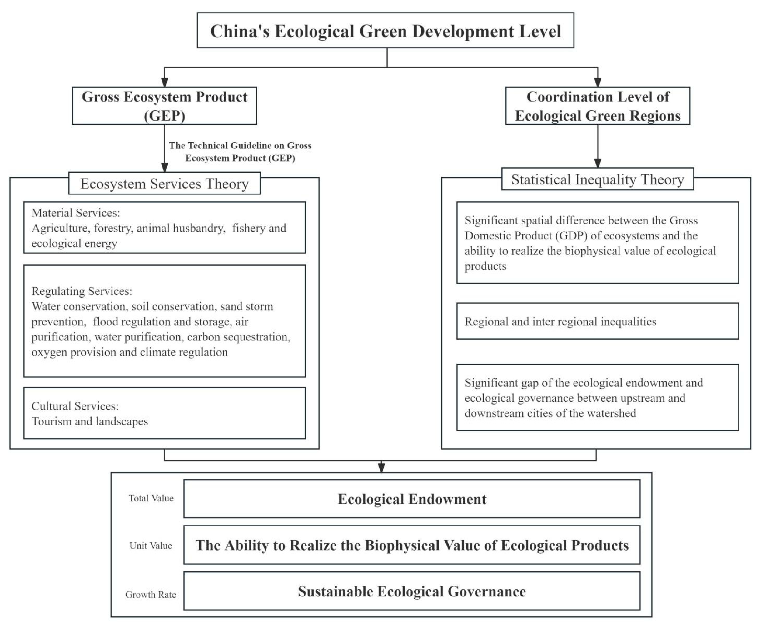
Figure 1. Framework for China’s eEological Green Development Level.
Sustainability 17 04451 g001
Figure 2. Trend of GEP and its subordinate indicators at national level (the units of all monetary value are in “trillion yuan”).
Sustainability 17 04451 g002
Figure 3. Trend of subordinate indicators in Regulation Services in China (the units of all monetary value are in “trillion yuan”).
Sustainability 17 04451 g003
Figure 4. Trend of GEP in the western, central and eastern regions in city level (The monetary value is the average GEP of the cities within this region. The units of GEP are in “Hundred million yuan” and the units of GEP per unit area are in “yuan per square meter”).
Sustainability 17 04451 g004
Figure 5. Trend of subordinate indicators of GEP in the western, central and eastern region (The monetary value is the average level of the cities within this region. The units of Material Product Supply, Regulation Services and Cultural Services are in “Hundred million yuan” and the units of monetary value of Regulation Services per unit area are in “yuan per square meter”.).
Sustainability 17 04451 g005
Figure 6. Within-group Gini coefficient in the western, central and eastern region.
Sustainability 17 04451 g006
Figure 7. Between-group Gini coefficients between the western, central and eastern regions.
Sustainability 17 04451 g007
Figure 8. Kernel density estimation of GEP and its subordinate indicators at national level.
Sustainability 17 04451 g008
Figure 9. Scatter plot of Moran’s I.
Sustainability 17 04451 g009
Table 1. The total value of indicators (CNY trillion).
YearGEPGDPMaterial Product SupplyRegulation ServicesCultural Services
200547.1718.602.1443.551.48
200852.3132.123.0146.702.60
201154.4948.344.2845.215.00
201461.8164.445.2447.958.62
201564.1468.565.4748.729.95
201766.4183.095.6046.5414.27
202074.40100.556.9148.7218.77
Note: The units of all indexes are “trillion yuan”. The Gross Ecological Product (GEP), the monetary value of material products provided, the monetary value of Regulation Services, and the monetary value of Cultural Services are calculated by the author, while the Gross Domestic Product (GDP) data are sourced from the National Bureau of Statistics.
Table 2. Monetary value of Regulation Services for ecosystems (CNY trillion).
YearForest EcosystemWetland EcosystemGrassland EcosystemFarmland Ecosystem
Monetary ValueAreaMonetary ValueAreaMonetary ValueAreaMonetary ValueArea
200534.53229.95 4.44 13.74 3.91 191.52 0.61 287.18
200838.08 231.71 3.87 14.03 4.07 189.34 0.60 287.31
201136.76 232.55 3.58 14.25 4.34 188.73 0.46 286.23
201439.39 231.67 3.90 14.44 4.03 190.19 0.56 283.84
201739.11 233.60 4.71 14.41 4.10 188.44 0.70 281.93
202034.53 229.95 4.44 13.74 3.91 191.52 0.61 287.18
Note: The monetary value of each ecosystem is measured in “trillion yuan”, and the area is measured in “ten thousand square kilometers.” The values are calculated by the author, and the areas of each ecosystem are derived from land use data. This table only lists the ecosystem categories most relevant to ecosystem regulation and service functions, with forest ecosystems including both woodland and shrubland.
Table 3. Monetary value of indicators in each province (CNY hundred billion).
ProvinceGEPRegulation ServicesValue
per Area
ProvinceGEPRegulation ServicesValue
per Area
Beijing4.761.317.57Hubei25.4220.0113.97
Tianjin0.410.233.04Hunan41.1735.1819.60
Hebei15.509.474.94Guangdong28.3725.673.44
Shanxi0.580.451.64Guangxi58.6353.2125.39
Inner Mongolia55.5746.3529.64Hainan0.730.5327.82
Liaoning15.7810.456.68Chongqing1.701.362.57
Jilin11.288.425.09Sichuan29.1021.0311.69
Heilongjiang25.4422.044.91Guizhou8.856.4512.21
Shanghai3.260.357.01Yunnan31.3528.6816.45
Jiangsu19.129.049.23Tibet11.518.195.12
Zhejiang28.6220.6821.98Shaanxi20.6917.218.46
Anhui20.9215.6412.00Gansu10.168.792.24
Fujian34.7730.4527.82Qinghai2.290.252.45
Jiangxi40.6135.8223.47Ningxia0.660.341.38
Shandong18.109.336.04Xinjiang14.9112.0515.64
Henan17.4510.486.57
Note: The units of all indexes are “hundred billion yuan”. The monetary values of Regulation Services per unit area are “yuan per square meter”. Provinces are sorted by province code.
Table 4. The results of Global Moran’s I.
YearProximity Weight MatrixDistance Weight Matrix
IZIZ
20050.425 ***10.6460.084 ***0.005
20060.481 ***11.9840.102 ***0.005
20070.357 ***9.0990.066 ***0.005
20080.441 ***11.0560.089 ***0.005
20090.449 ***11.1660.092 ***0.005
20100.431 ***10.7880.085 ***0.005
20110.374 ***9.480.067 ***0.005
20120.429 ***10.7350.085 ***0.005
20130.395 ***9.9560.075 ***0.005
20140.379 ***9.5720.077 ***0.005
20150.382 ***9.6420.076 ***0.005
20160.391 ***9.8060.083 ***0.005
20170.367 ***9.2540.078 ***0.005
20180.353 ***8.8920.071 ***0.005
20190.375 ***9.4080.079 ***0.005
20200.349 ***8.8090.078 ***0.005
Note: The I value, also known as Global Moran’s I value, is an indicator that measures the spatial autocorrelation of the entire region, *** significant at the 1% level. The Z-value is a standard score used to measure the difference between observed values and expected values (i.e., values under a random distribution). It reflects the degree to which Global Moran’s I deviates from the null hypothesis (i.e., the data are randomly distributed).
Disclaimer/Publisher’s Note: The statements, opinions and data contained in all publications are solely those of the individual author(s) and contributor(s) and not of MDPI and/or the editor(s). MDPI and/or the editor(s) disclaim responsibility for any injury to people or property resulting from any ideas, methods, instructions or products referred to in the content.