Method to Select Variables for Estimating the Parameters of Equations That Describe Average Vehicle Travel Speed in Downtown City Areas

Abstract

A lack of public vehicular traffic data for a city limits our understanding of the traffic occurring in the street networks of that city; however, there are free tools to extract street network graphs from digital maps and to assess the static properties associated with those graphs. This study proposes a two-stage modeling method to describe dynamic traffic data with static street network features. A quadratic polynomial is used to fit the average travel speed (ATS) pattern observed in the city center. Then, the relationship between the polynomial parameters and street network variables is analyzed through multiple linear regression. Descriptive geometric and topological measurements of downtown areas are obtained with the OSMnx tool (from OpenStreetMap), and with these data, independent variables are defined. The speed of vehicles, assessed every 15 min (from 6:00 a.m. to 10:00 p.m.) on the downtown street networks of twelve major cities, is obtained with the distance_matrix service of GoogleMaps, and with these data, the ATS (the dependent variable) is calculated. The ATS (presenting a U-shape) is modeled with a polynomial equation of order two, so there are three parameters for each city; in turn, each parameter is modeled with a multiple linear regression equation with the independent variables. For training purposes, the ATS equation parameters of ten cities are calculated, and the parameters, in turn, are explained with the proposed method. For validation purposes, the parameters of two cities not considered in the training process are calculated with the multiple linear regression equations. The ATS equation parameters of the twelve cities are correctly modeled so that each city’s ATS can be adequately described. It was concluded that the method selects the independent variables that are suitable to explain the ATS equation parameters. In addition, with the Akaike information criterion, the variable selection case presenting the best trade-off between accuracy and complexity is identified.

1. Introduction

The speeds at which vehicles circulate in the downtown areas of major cities in many countries have not yet been described properly. The principal reason for this is the lack of technology, i.e., the required infrastructure to measure traffic conditions. Fortunately, with the era of information technology, there are now some options. OpenStreetMap (OSM) contains a lot of information from networks (topological and geometrical) that can be extracted. Additionally, GoogleMaps offers services to deliver data that can be used as a proxy of direct speed measurements in the field. The focus of this work is to develop a method to determine which static street network features can be selected as inputs of a process whose output is the average vehicle speed in street networks of downtown areas.

In order to preserve the geometric patterns and geographical properties [1,2,3] of the street networks used in this study, the primal approach (where street segments are links and intersections are nodes) was used to represent them, which is a natural approach [4]. The differences between the primal approach and the dual approach are outlined in [2], where it was concluded that the primal approach captures (in greater detail than the dual) centrality information details to describe the network structure, and that the distribution of centrality is different between self-organized and planned cities. Topological and geometric network measurements are widely used in urban planning and transportation practice. Three supplemental measurements were proposed in [5], i.e., measurements of entropy, connection patterns (by measuring ringness, webness, beltness, circuitness, and treeness), and continuity (which evaluates the network quality from a driver’s perspective). A summary of research on network measurements for describing the topological characteristics of transportation networks is given in [3].

The literature suggests that static street network characteristics can explain traffic conditions to some extent. The correlation between traffic flow and centrality measurements at different modes (point mode, line mode, and area mode) was studied in [6], where it was found that modified centrality measurements presented a higher correlation with traffic flow than the conventional measurements; for similar works, see [7,8]. In the present work, in order to better approximate observations and estimations, it was deemed suitable to use multiple independent variables (the static street network characteristics) to explain the dependent variable (average travel speed). In [9], the traffic flow (the dependent variable) was better explained with multiple linear regression than with univariate analysis or other multivariate approaches (random forest, support vector regression, or artificial neural networks). The topological measurements used in [9] were degree, betweenness, closeness, page rank, and the clustering coefficient, and the geometrical property was road length, which altogether were the independent variables.

Speed estimations are important in mobility applications, such as for defining travel routes and forecasting travel times [10]. To estimate the free-flow speed on links without considering diurnal speed fluctuations, see [11,12]. The use of street network properties to predict vehicle speed on network links is discussed in [13]; the independent variables in that study were speed limit, betweenness (to identify important links), and closeness (to distinguish between central urban and peripheral rural streets), and the model coefficients were calculated to explain vehicle speed (the dependent variable) for a given time interval and street category. The model presented in [14] estimates the speed on a road link considering diurnal variation throughout a day; the independent variables were daytime, the functional road classification, and the legal speed limit (the map attributes were extracted from OSM). That study also discussed the transferability of the model to another comparable region (similar in topography, peak hours, traffic demand, and driving behavior).

A macroscopic cost flow function in the form of the macroscopic bureau of public roads (MBPR) was formulated with network topological metrics, as in reference [15]; the free flow travel time was correlated with the average number of junctions per unit of distance and the congestion sensitivity parameter with the road density. Therefore, the network average travel time depended on traffic demand and the spatially variable network topological features. The relation between network topologies and the network macroscopic fundamental diagram (MFD) was modeled in the form of a macroscopic Underwood’s model [16]. With this model, the space mean speed over time period T was explained by the free-flow space mean speed, the traffic density per unit of area, and the optimal density per unit of area. The free-flow space mean speed was explained by the average number of junctions per unit of distance (the first decreased as the second increased), and the optimal density was explained by the density degree normalized by the trafficable area. A sensitivity analysis suggested that the found relationships may be true on networks of different size. That work focused on traffic modeling considering static street network features as explanatory variables; however, the attempts at speed predictions with new techniques, for example, with deep learning [17,18,19] and with graph neural networks [20,21,22], are notorious.

The present work is different from the ones revised in literature. In our approach, the speed of individual street links was calculated considering time. Every 15 min (from 6:00 a.m. to 10:00 p.m.), an average was calculated that represent the traffic speed conditions of downtowns zones. With a second order equation, the average travel speed (ATS) was described, and the parameters of these equations estimated following the proposed method, with street network metrics as the independent variables. The source of the data used in the present work was a low-cost alternative, as an extensive measurement campaign was not feasible.

The research questions are as follows:

• Can static street network features be used as independent variables to describe the average travel speeds in downtown zones?
• Which is the best method to determine the independent variables that might be used to estimate the parameters of the equations that describe the ATS?

A summary of the methodology used in this study is presented in Figure 1.

Figure 1. Summary of the used methodology as a block diagram.

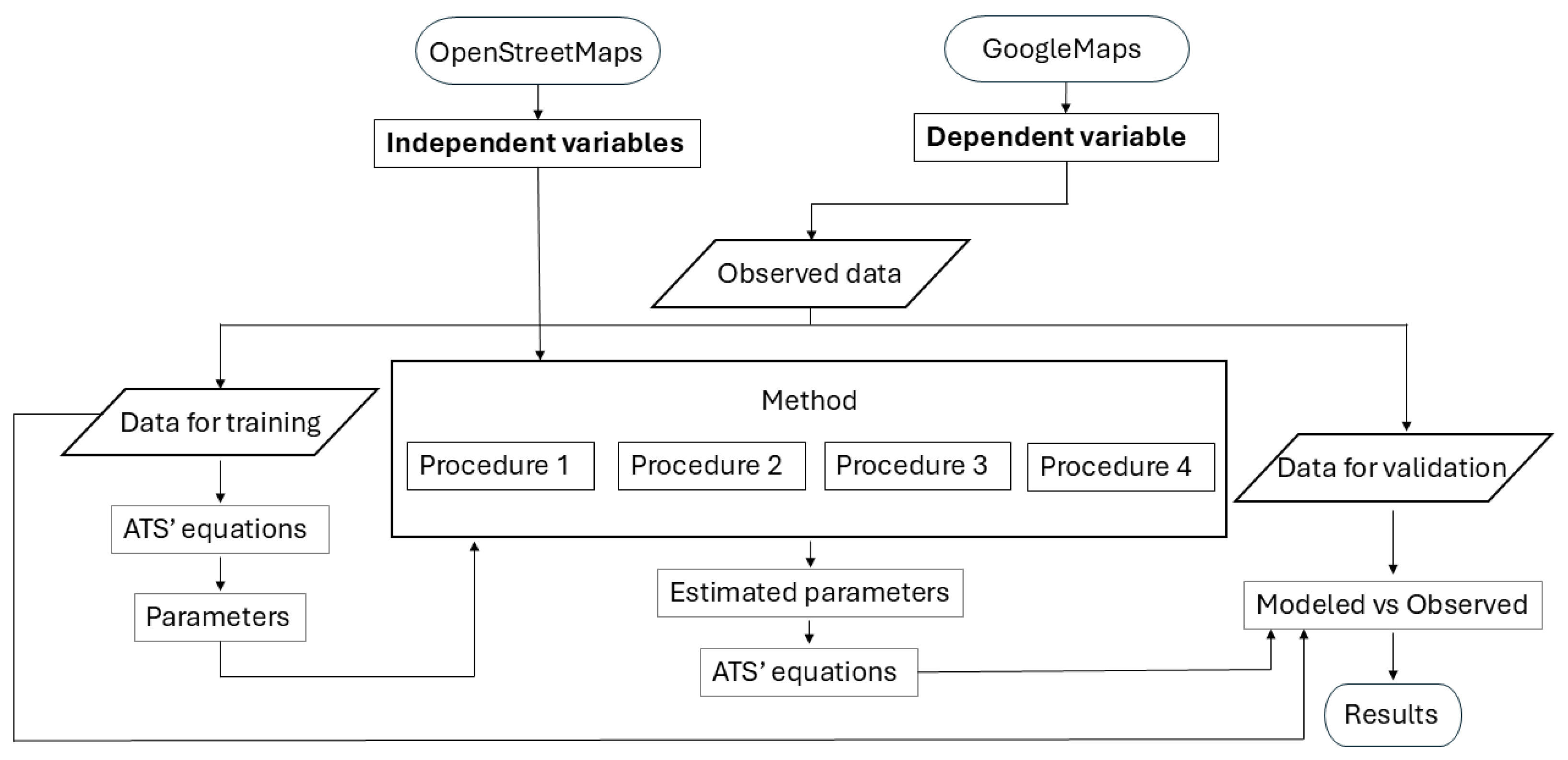
2. Materials and Methods

The selected Mexican cities for this investigation were Toluca, Puebla, Queretaro, San Luis Potosi, Aguascalientes, Durango, Guadalajara, Mazatlan, Monterrey, Veracruz, Ciudad de Mexico, and Merida. The TomTom company calculates the average travel time (ATT) required to travel 10 km. For example, in Ciudad de Mexico, ATT = 31 min 53 s; for Puebla, ATT = 29 min 57 s; for Guadalajara, ATT = 27 min 8 s; and for Monterrey, ATT = 18 min 21 s. These cities were selected due to their positions in the TomTom traffic index 2024 rankings [23]. For completeness, other cities without serious congestion problems were also selected.

For each city, a (central) point in the downtown zone was selected, and from this point, a 500 m radius was identified to establish the area under analysis. Table 1 shows the latitude and longitude of the central points, the dates on which the traffic information was acquired, and the id (identifier) of each city.

Table 1. Cities’ central point coordinates and dates on which the traffic information was obtained.

City	Latitude, Longitude (central_point)	Readings’ Date (year/month/day)	id
Toluca	19.290271, −99.656241	2024/4/10	1
Puebla	19.045296, −98.199224	2024/5/8	2
Queretaro	20.591938, −100.393755	2024/5/22	3
San Luis Potosi	22.152679, −100.977041	2024/4/10	4
Aguascalientes	21.883707, −102.295368	2024/4/10	5
Durango	24.025159, −104.667530	2024/4/3	6
Guadalajara	20.674257, −103.350420	2024/4/10	7
Mazatlan	23.202669, −106.420695	2024/5/22	8
Monterrey	25.676165, −100.314396	2024/5/22	9
Veracruz	19.196422, −96.137607	2024/5/29	10
Ciudad de Mexico	19.432574, −99.133204	2024/5/8	11
Merida	20.967084, −89.623739	2024/5/29	12

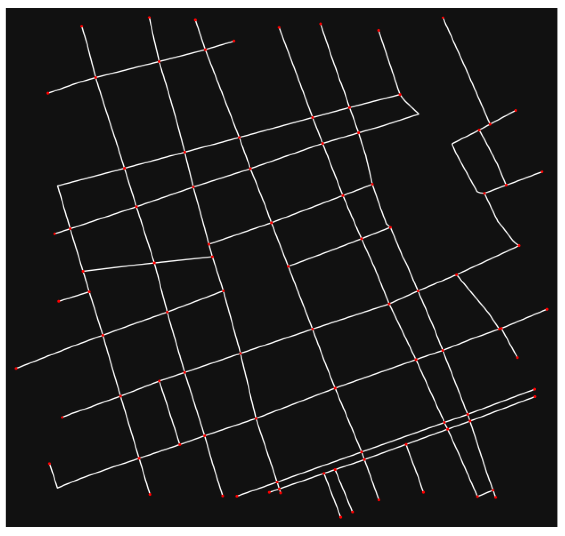
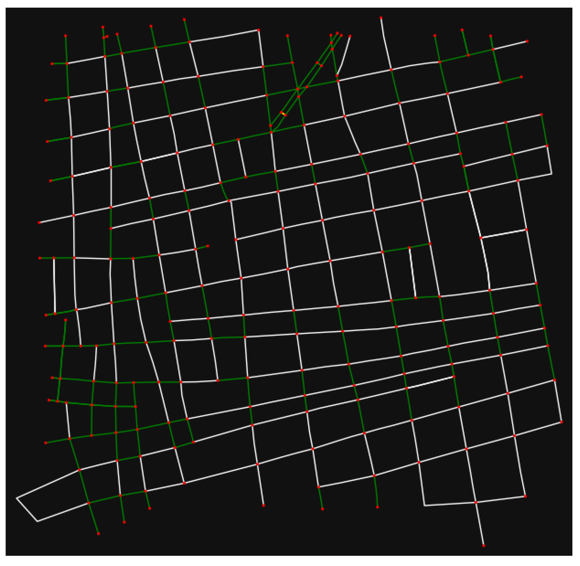
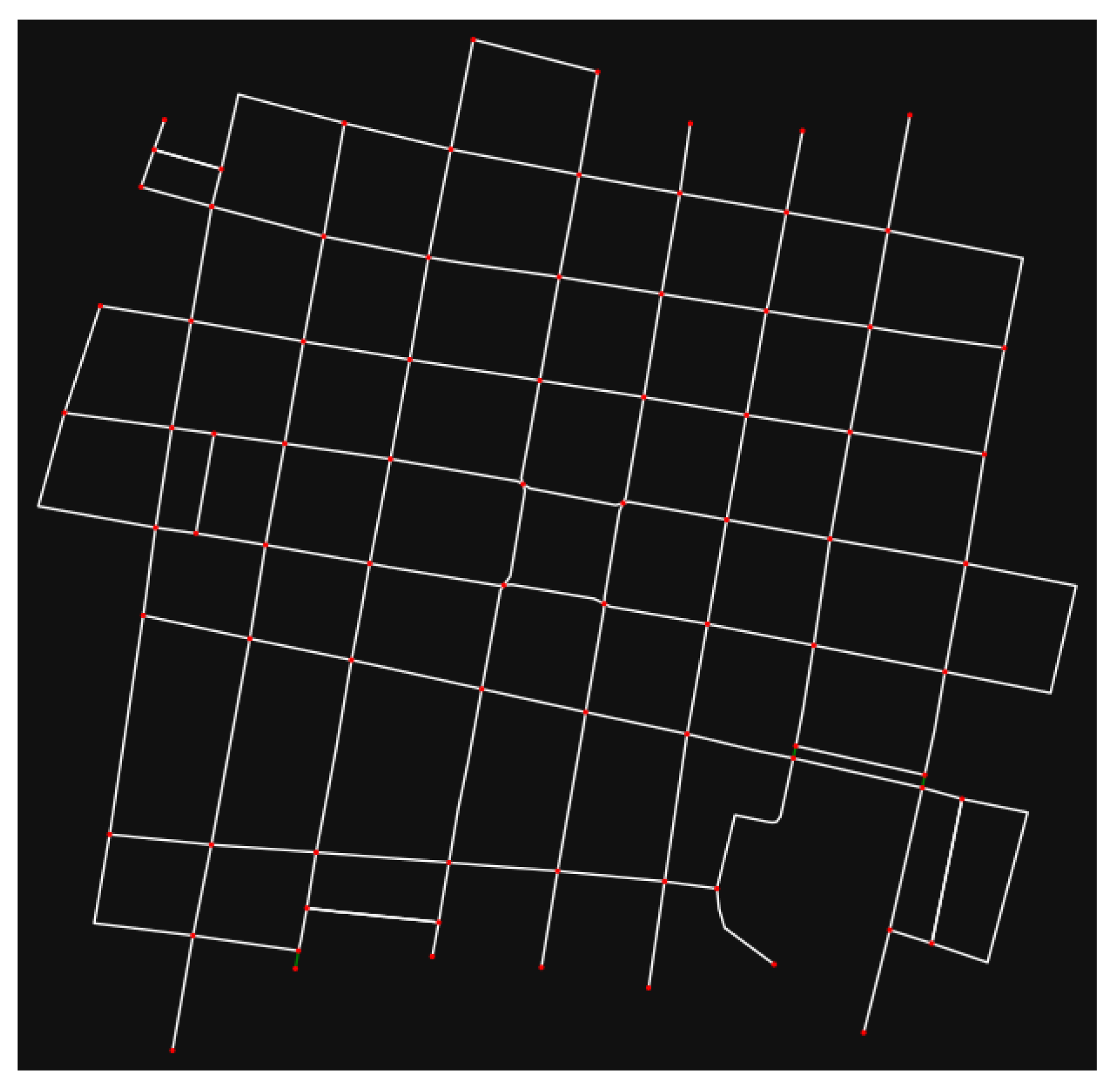
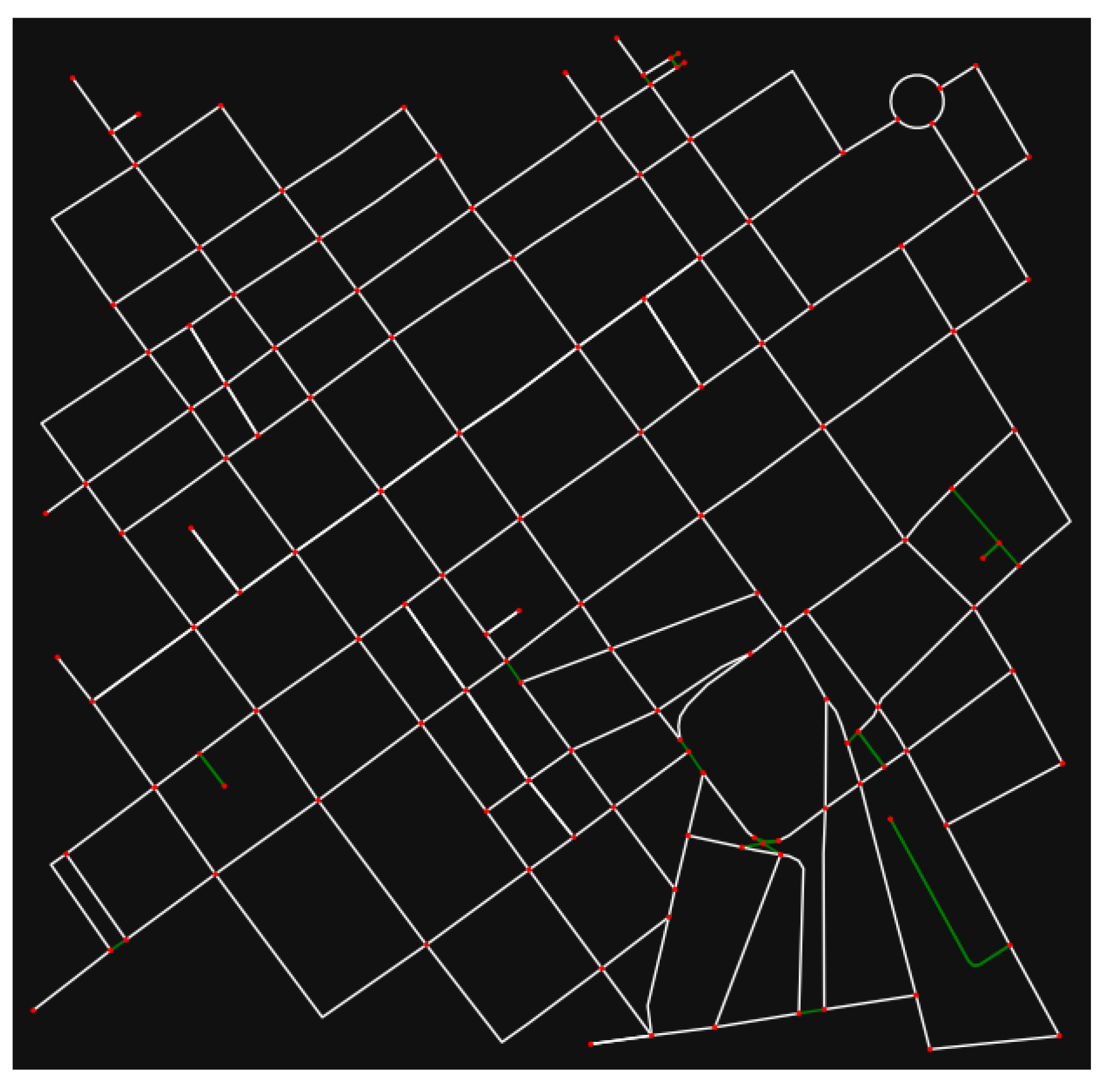
2.1. Instructions to Extract Street Network Data

With the OSMnx tool, the street networks were downloaded from OpenStreetMap [24]. The static street network characteristics of each city could be obtained through Technique 1 or Technique 2 (see Appendix A.1). All the programming instructions presented in this paper were implemented with Python 3.11.2.

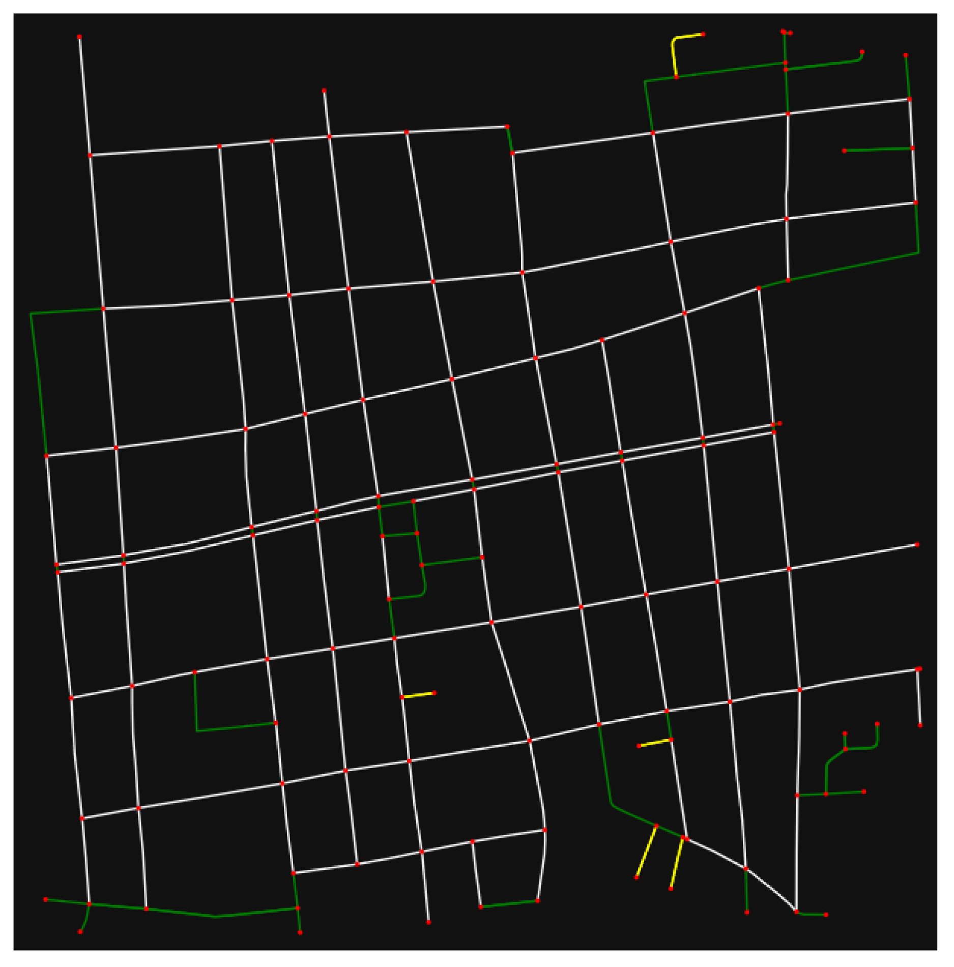
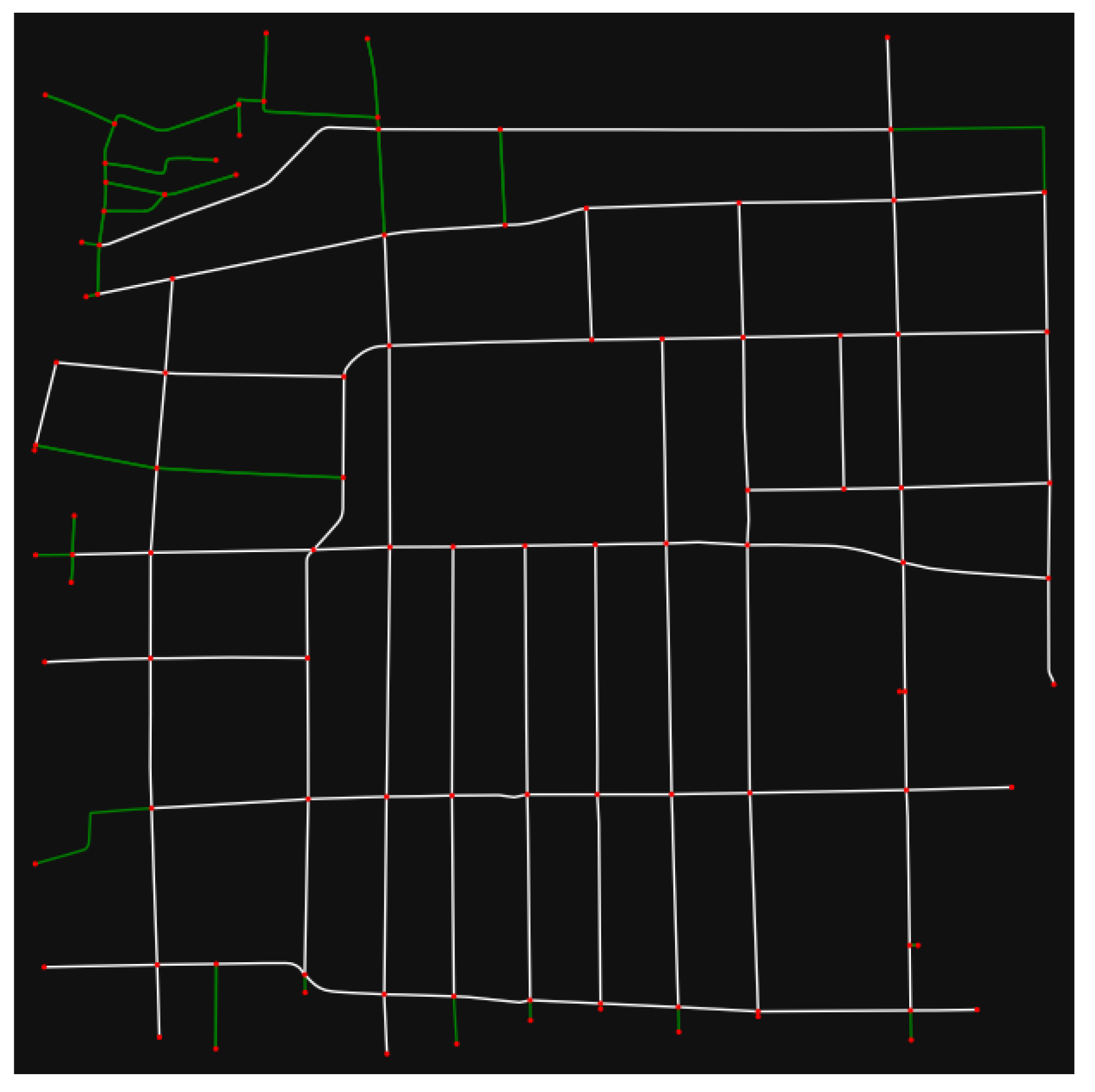
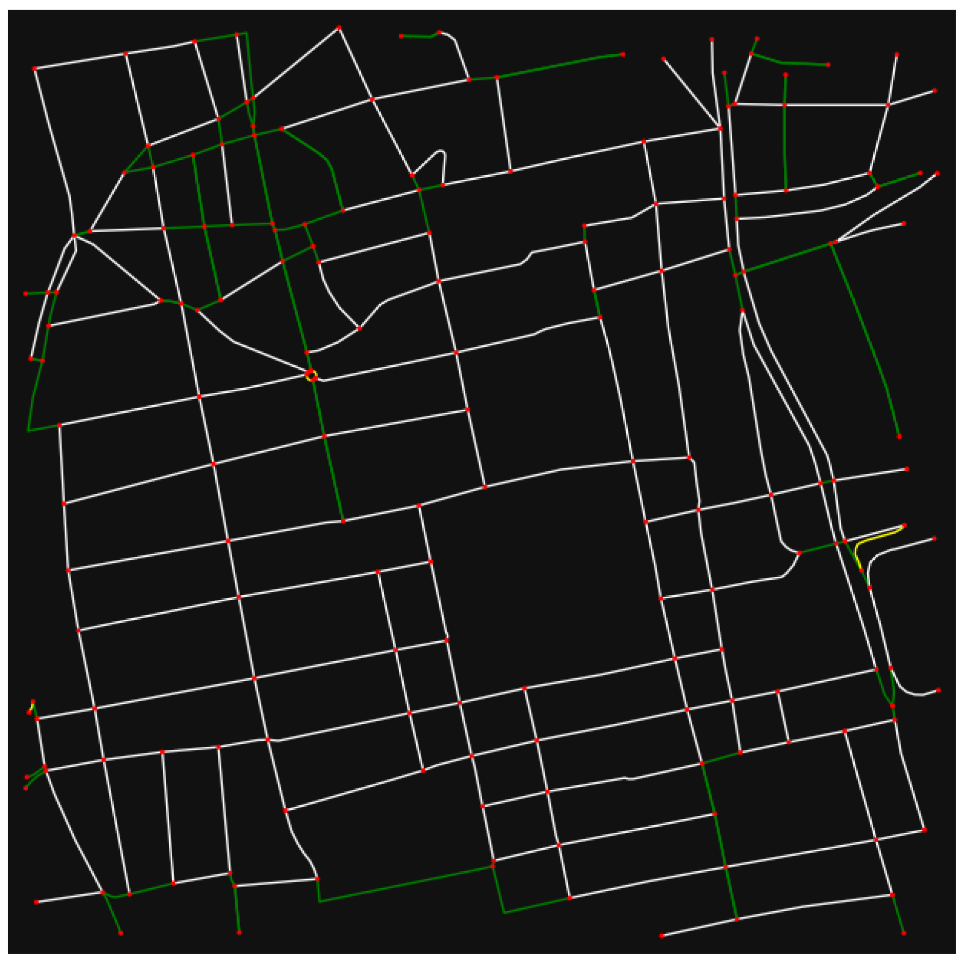
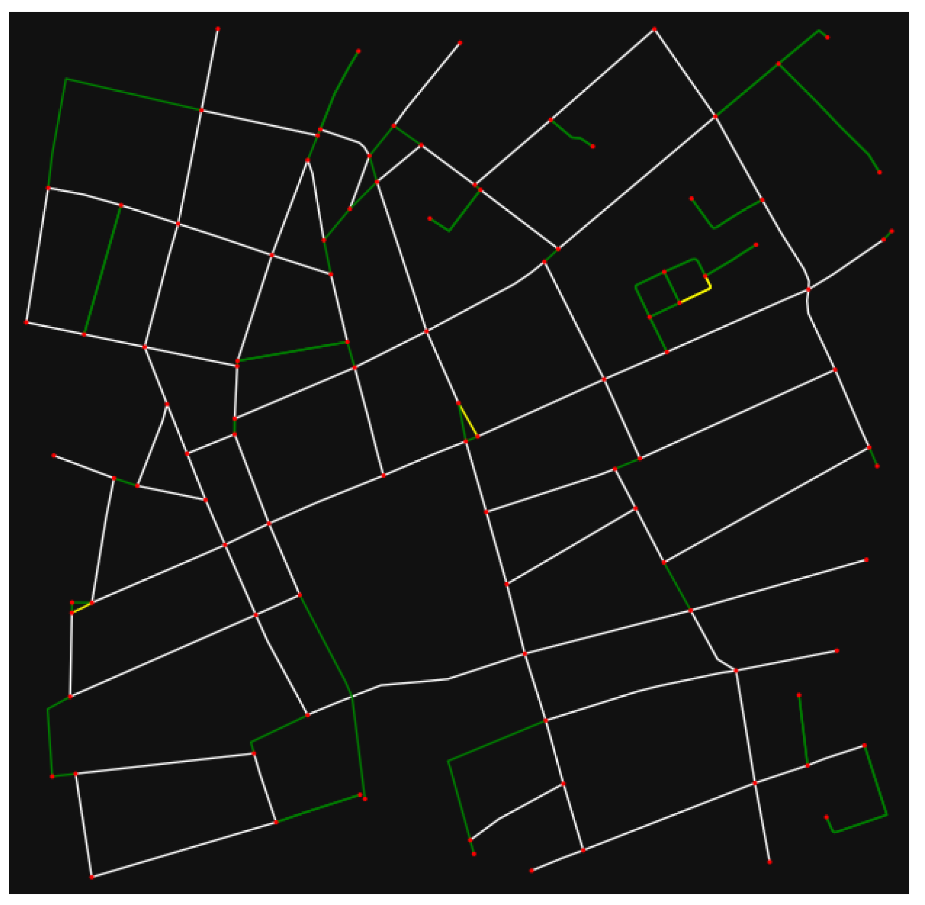
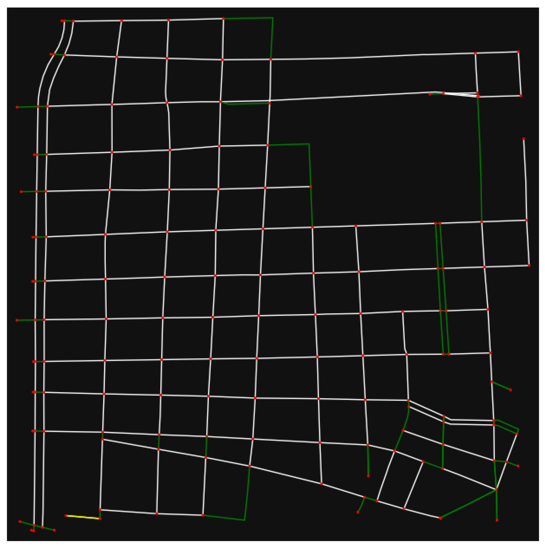
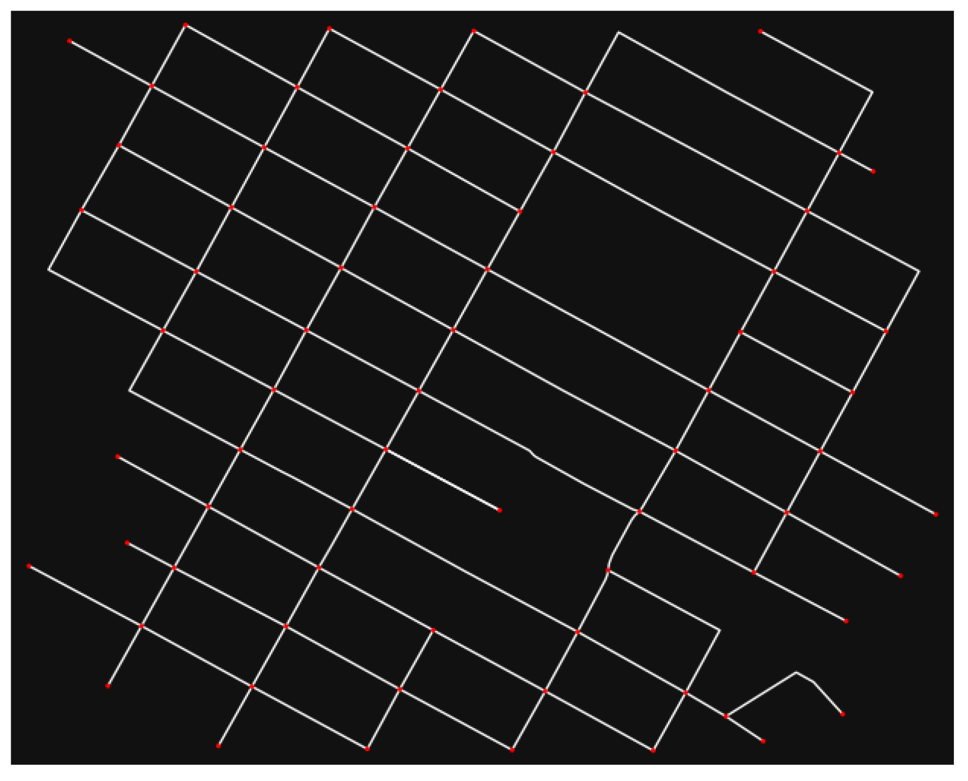
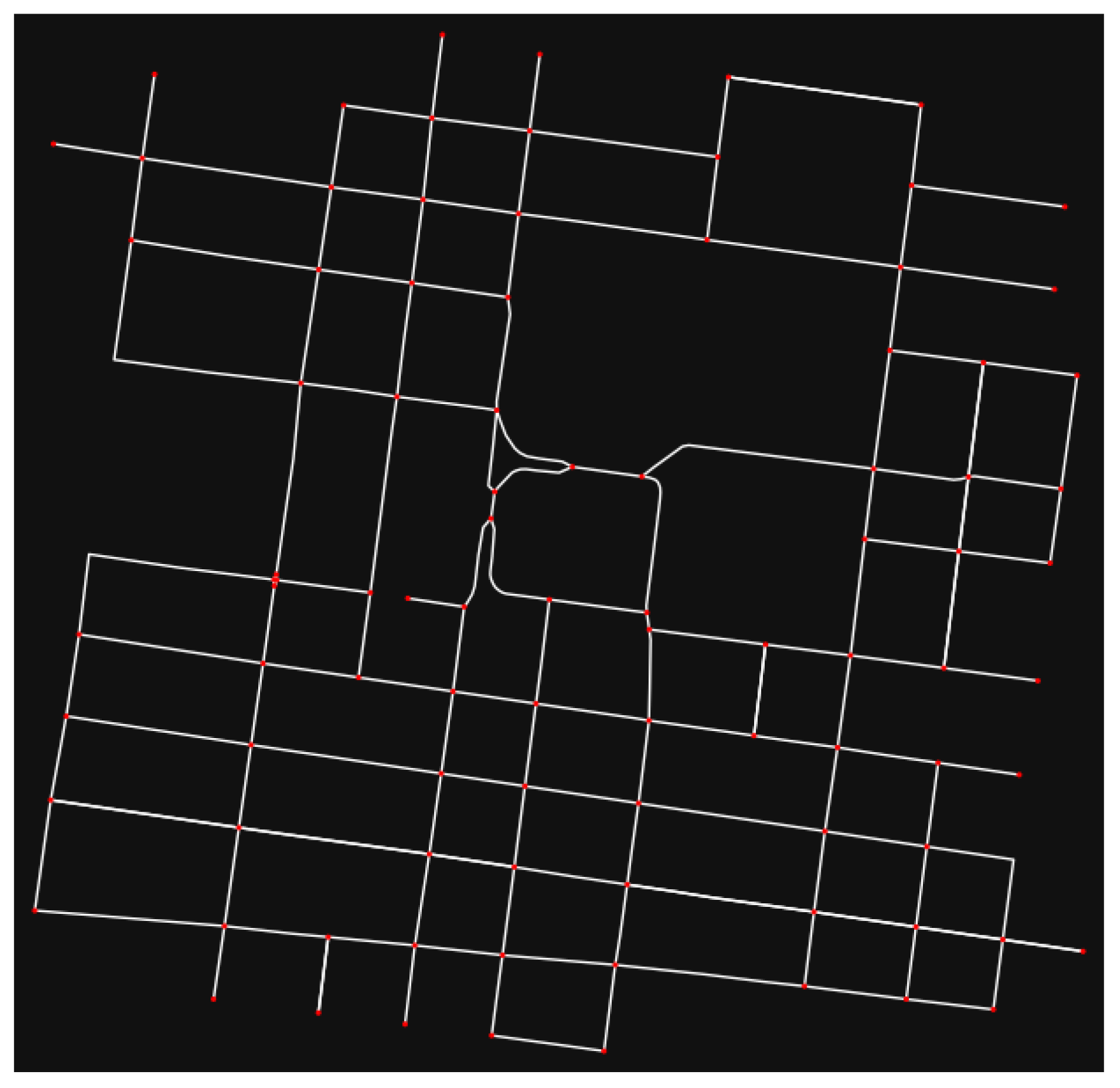
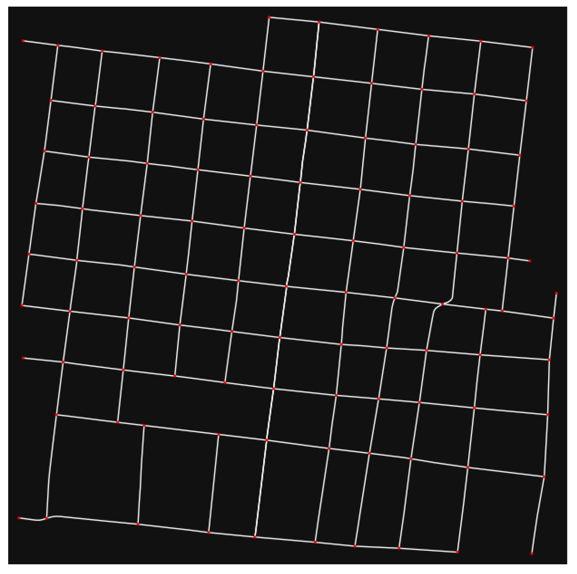
2.2. Street Networks of Cities

In Appendix A.2, a graph of each city is presented, as well as the edges used to acquire speed readings.

2.3. Speed Measurements

To acquire speed readings on a selected edge, a service provided by GoogleMaps was used in the form of the following instruction:

output = gmaps.distance_matrix((n1_latitude, n1_longitude), (n2_latitude, n2_longitude), mode = ‘driving’, units = ‘metric’, departure_time = d_t, traffic_model = ‘best_guess’)

where n1 and n2 are the nodes at the edge ends, n1_latitude and n1_longitude are the latitude and longitude of n1, respectively, and n2_latitude and n2_longitude are the latitude and longitude of n2, respectively. The variable d_t = (year, month, day, hour), the year, month, and day are as presented in Table 1. The first data request happened at hour = 6 a.m. and subsequent requests were made every 15 min, the instruction d_t = d_t + datetime.timedelta(minutes = 15) was used to update d_t. The last data request was performed at hour = 10 p.m. The other arguments of gmaps.distance_matrix can be consulted in [25]. The distance (distance) to go through an edge and the travel time (travel_time) needed to complete that distance were obtained as follows:

distance = output[‘rows’][0][‘elements’][0][‘distance’][‘value’]

travel_time = output[‘rows’][0][‘elements’][0][‘duration_in_traffic’][‘value’]

The travel speed (travel_speed) on the edge was calculated by travel_speed = distance/travel_time. Because the range in time for acquiring readings was from 6 a.m. to 10 p.m. at intervals of 15 min, the data of an edge had 65 travel speed samples. To corroborate if distance was equal to the edge length (edge_length) was calculated dif = abs(distance − edge_length); if $\mathrm{dif}<10$, no action was taken; if $\mathrm{dif}\ge 10$, the edge was removed from the analysis. The reason for this error was that the nodes coordinates of the edge did not exactly match between OpenStreetMap (from which the edges data were obtained) and GoogleMaps, so if $\mathrm{dif}\ge 10$, the route taken by gmaps.distance_matrix was not the one that strictly went along the edge.

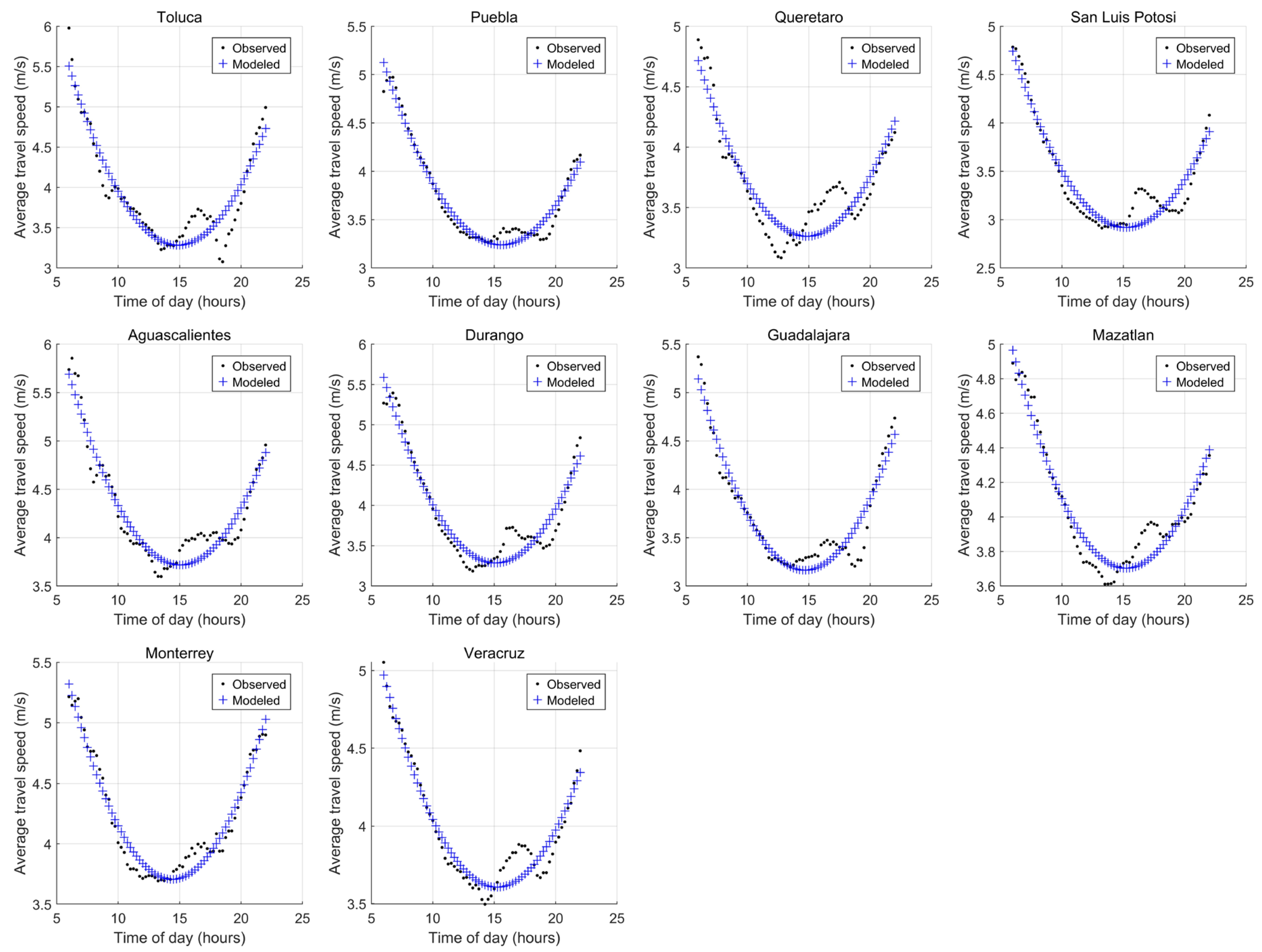
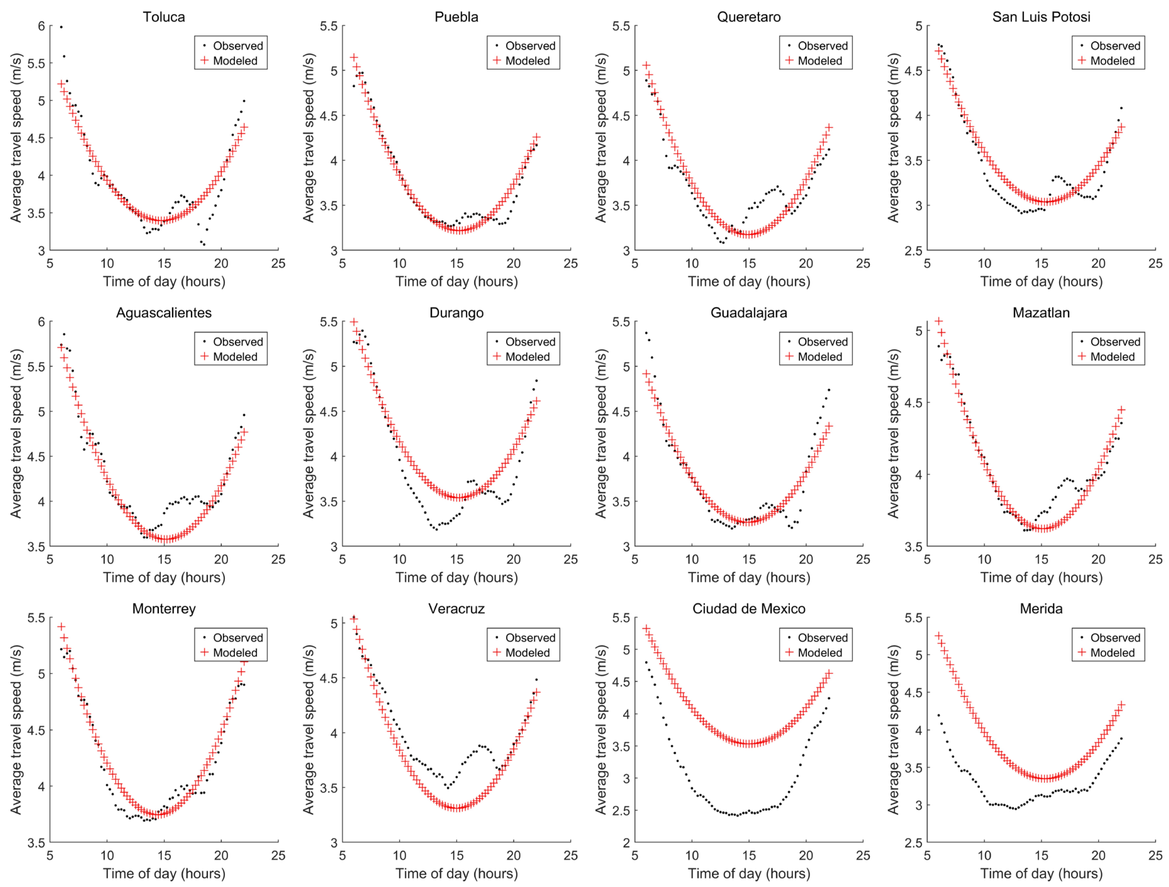
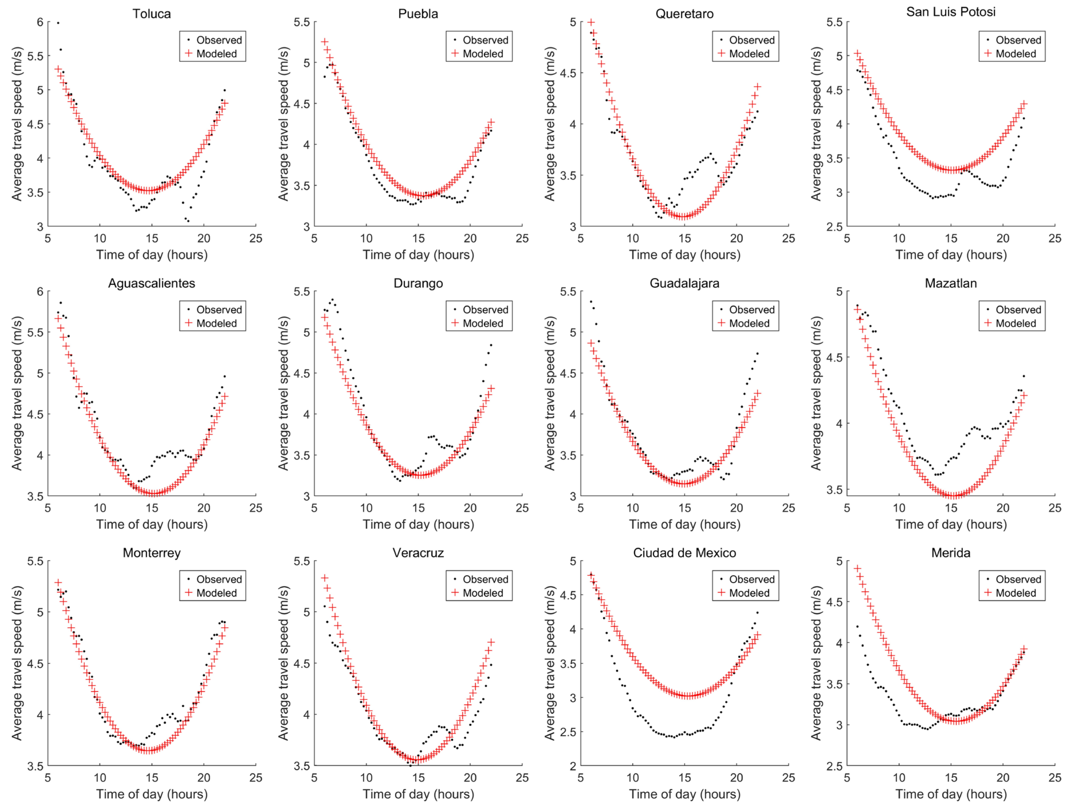
2.4. Model to Describe the Average Travel Speed (ATS)

For a city, for each point in time, the variable travel_speed was averaged using the segments of the city, resulting in the average travel speed (ATS). ATS_i as a function of time (i is the time index) was the pattern to be modeled. Hereafter, ATS_i will be referred to as the “observations”. This pattern had a U-shape that could be explained with a polynomial second order equation; see Equation (1). Higher order polynomials would have increased the complexity of the model and are beyond the scope of this work.

$$\mathrm{ATS}\_{\mathrm{MOD}}_{\mathrm{i}}={\mathrm{at}}^2+\mathrm{bt}+\mathrm{c}$$

(1)

In Equation (1), $\mathrm{ATS}\_{\mathrm{MOD}}_{\mathrm{i}}$ is the modeled average travel speed, t represents a point of time inside the range under evaluation, and i is the time index associated with t. The three parameters, a, b and c for each city, could then be estimated. The intention was to describe each parameter by the street network data with multiple linear regression. Ten cities were selected to train the model: Toluca (id = 1), Puebla (id = 2), Queretaro (id = 3), San Luis Potosi (id = 4), Aguascalientes (id = 5), Durango (id = 6), Guadalajara (id = 7), Mazatlan (id = 8), Monterrey (id = 9), and Veracruz (id = 10). The parameter values of Equation (1) of each city are shown in Table 2.

Table 2. Parameter values of the ATS equations.

City	Parameter a	Parameter b	Parameter c	MAE 1 (m/s)
Toluca	0.028396	−0.843706	9.547877	0.165484
Puebla	0.020665	−0.642999	8.239078	0.078630
Queretaro	0.0186069	−0.552343	7.360227	0.146007
San Luis Potosi	0.021510	−0.654421	7.895163	0.118764
Aguascalientes	0.0240903	−0.725108	9.173014	0.132317
Durango	0.0278565	−0.840950	9.630438	0.148438
Guadalajara	0.026250	−0.770993	8.823447	0.121535
Mazatlan	0.014890	−0.452952	7.146595	0.076942
Monterrey	0.022889	−0.659153	8.451607	0.087286
Veracruz	0.016063	−0.488818	7.324627	0.079215

¹ MAE is the Mean Absolute Error.

Table 2 also presents the Mean Absolut Error (MAE), which was calculated with Equation (2):

$$\mathrm{MAE}={\displaystyle \frac{{\sum }_{\mathrm{i}=1}^{\mathrm{n}}\left|{\mathrm{ATS}}_{\mathrm{i}}-\mathrm{ATS}\_{\mathrm{MOD}}_{\mathrm{i}}\right|}{\mathrm{n}}}$$

(2)

where i is the time index and n = 65. Figure 2 shows, for each city, the observed ATS in black dots and the modeled ATS_MOD in blue. It can be observed that for some cities, the ATS resembles a W-shape. Nevertheless, the ATS_MOD was close enough to the ATS, and as such, a model considering one change of direction using a second order equation was deemed to be adequate.

Figure 2. Observed (ATS) vs. modeled (ATS_MOD) as a function of time.

2.5. Independent Variables

Next, we sought to explain ATS equation parameters a, b, and c by the street network variables in Table 3. See reference [24] for definitions of the variables with ID = 1 to 6. The road classification tag description of OpenStreetMap is in reference [26].

Table 3. Street network variables.

Variable	Definition	ID
n	The number of nodes in the network.	1
m	The number of edges in the network.	2
k_avg	Average node degree (in-degree and out-degree).	3
sum_edges_length	The sum of the edge length in the network (in meters).	4
avg_edges_length	The average of the edge length (in meters).	5
circuity_avg	The total edge length divided by the sum of great circle distances between the nodes incident to each edge.	6
oneway_true	The percentage of one-way edges.	7
length _75	The percentage of edges with a length ≤ 75 m.	8
length _125	The percentage of edges with a length > 75 m and ≤125 m.	9
length _ leftover	The percentage of edges with a length > 125 m.	10
h_residential	The percentage of edges classified as residential.	11
h_tertiary	The percentage of edges classified as tertiary.	12
h_ leftover	The sum of the following percentages: % of edges classified as primary + secondary % + living_street % + trunk % + primary_link % + secondary_link % + tertiary_link %.	13
lanes_1	The percentage of edges with 1 lane.	14
lanes_2	The percentage of edges with 2 lanes.	15
lanes_ leftover	The sum of: % of edges with 3 lanes + % with 4 lanes + % with 5 lanes + % with 6 lanes.	16
intercept	The constant term equal to 1.	17

The values of the variables presented in Table 3 are presented in Table 4 (the units of the variables are specified in Table 3). The values of the variables in Table 4 were normalized to be in the range from 0 to 1.

Table 4. Independent variable values.

	Variable ID
City	1	2	3	4	5	6	7	8	9	10	11	12	13	14	15	16
Toluca	97	159	3.27835	16,617.4190	104.5120	1.0097	0.6981	0.3962	0.2830	0.3207	0.5838	0.1118	0.3043	0.0097	0.3106	0.6796
Puebla	68	105	3.0882	16,339.4670	155.6139	1.0318	0.9809	0.0285	0.4571	0.5142	0.4363	0.1363	0.4272	0.0740	0.9259	0
Queretaro	94	130	2.7659	15,400.8590	118.4681	1.0175	1	0.2461	0.2538	0.5000	0.7022	0.0534	0.2442	0.1153	0.3269	0.5576
San Luis Potosi	186	308	3.3118	22,967.7810	74.5707	1.0127	0.7987	0.5844	0.2694	0.1461	0.7419	0.0258	0.2322	0.2261	0.7619	0.0119
Aguascalientes	77	110	2.8571	12,447.2360	113.1566	1.0256	1	0.3181	0.3181	0.3636	0.3839	0.3571	0.2589	0.1578	0.8157	0.0263
Durango	110	181	3.2909	16,980.1849	93.8131	1.0147	0.9447	0.4198	0.2762	0.3038	0.5879	0.3021	0.1098	0	0.9636	0.0363
Guadalajara	145	247	3.4068	20,779.2279	84.1264	1.0087	0.9352	0.3076	0.6234	0.0688	0.7935	0.0121	0.1943	0.2460	0.4047	0.3492
Mazatlan	220	391	3.5545	29,011.3119	74.1977	1.0132	0.8465	0.4808	0.4936	0.0255	0.8081	0.1867	0.0051	0	1	0
Monterrey	103	185	3.5922	18,577.7809	100.4204	1.0008	0.9027	0.0540	0.8594	0.0864	0.5621	0.1351	0.3027	0.0823	0.2117	0.7058
Veracruz	140	245	3.5000	20,149.0319	82.2409	1.0267	0.8122	0.4897	0.3836	0.1265	0.6491	0.0887	0.2620	0	0.6666	0.3333
Ciudad de Mexico	93	154	3.3118	18,876.1639	122.5724	1.0189	0.8311	0.0454	0.6558	0.2987	0.6580	0.1935	0.1483	0.1393	0.7622	0.0983
Merida	82	137	3.3414	18,445.1519	134.6361	1.0457	0.9562	0.1094	0.1824	0.7080	0.6428	0.2285	0.1285	0.4824	0.5175	0

3. Results

The procedures for explaining the ATS equation parameters are presented in this section, along with the results.

3.1. Procedure 1: Selecting Variables Considering the ATS Error

Parameters a, b, and c, presented in Table 2, can be explained by multiple linear regression (MLR) considering the variables in Table 3. The vector $\mathrm{A}=\left[{\mathrm{a}}_1,{\mathrm{a}}_2\dots {\mathrm{a}}_{10}\right]$ contains parameter a for each city, and the sub index is associated with the id of the city, so ${\mathrm{a}}_1$ is the parameter of Toluca, ${\mathrm{a}}_2$ of Puebla, and so on. The same logic applies to vectors $\mathrm{B}=\left[{\mathrm{b}}_1,{\mathrm{b}}_2\dots {\mathrm{b}}_{10}\right]$ and $\mathrm{C}=\left[{\mathrm{c}}_1,{\mathrm{c}}_2\dots {\mathrm{c}}_{10}\right]$, which contain the b parameter values and the c parameter values, respectively. The parameters explained through the MLR were named _a, _b, and _c.

One or more variables from Table 3 can be selected as the independent variables for explaining a parameter in the MLR approach; see Equation (3).

$${\mathrm{y}}_{\mathrm{id}}={\mathsf{\beta }}_1{ \mathrm{x}}_{\mathrm{id},1}+{\mathsf{\beta }}_2{ \mathrm{x}}_{\mathrm{id},2}+\dots +{\mathsf{\beta }}_{\mathrm{p}}{ \mathrm{x}}_{\mathrm{id},\mathrm{p}}$$

(3)

where ${\mathrm{y}}_{\mathrm{id}}$ is the dependent variable (_a, _b, or _c), ${\mathsf{\beta }}_1$ to ${\mathsf{\beta }}_{\mathrm{p}}$ are the coefficients of the independent variables, ${\mathrm{x}}_{\mathrm{id},1}$ to ${\mathrm{x}}_{\mathrm{id},\mathrm{p}}$ are the independent variables (p variables from Table 3, so p is the number of independent variables), and id = 1…k is the city index (associated with the id presented in Table 1). With Equation (3) and p variables, $\_\mathrm{A}=\left[\_{\mathrm{a}}_1\dots \_{\mathrm{a}}_{10}\right]$, $\_\mathrm{B}=\left[\_{\mathrm{b}}_1\dots \_{\mathrm{b}}_{10}\right]$, and $\_\mathrm{C}=\left[\_{\mathrm{c}}_1\dots \_{\mathrm{c}}_{10}\right]$ were calculated. With these values, the average travel speed of each city was calculated, named $\_{\mathrm{ATS}}^{\mathrm{id}}$ for a specific city (the id corresponds to a city), e.g., for Toluca, $\_{\mathrm{ATS}}^1=\_{\mathrm{a}}_1{\mathrm{t}}^2+\_{\mathrm{b}}_1\mathrm{t}+\_{\mathrm{c}}_1$, or alternatively, $\_{\mathrm{ATS}}^{\mathrm{toluca}}=\_{\mathrm{a}}_1{\mathrm{t}}^2+\_{\mathrm{b}}_1\mathrm{t}+\_{\mathrm{c}}_1$. To measure the error ${\mathrm{E}}^{\mathrm{cities}}={\sum }_{\mathrm{id}=1}^{\mathrm{id}=\mathrm{k}}{\mathrm{E}}^{\mathrm{id}}$, see ${\mathrm{E}}^{\mathrm{id}}$ in Equation (4).

$${\mathrm{E}}^{\mathrm{id}}={\displaystyle \frac{{\sum }_{\mathrm{i}=1}^{\mathrm{n}}\left|{\mathrm{ATS}}_{\mathrm{i}}^{\mathrm{id}}-\_{\mathrm{ATS}}_{\mathrm{i}}^{\mathrm{id}}\right|}{\mathrm{n}}}$$

(4)

At this point, the second question emerged, i.e., Which variables could be used to estimate the parameters of the equations that describe the ATS? To address this, Algorithm 1 was introduced.

Algorithm 1. Generalized steps of Algorithm 1.

1. Among the variables in Table 3, the one for which ${\mathrm{E}}^{\mathrm{cities}}$ was the lowest was chosen as the first explicative variable. 2. In order to calculate ${\mathrm{E}}^{\mathrm{cities}}$, we considered all the variables that had already been selected along with one of the variables that not been selected yet (one at a time). Again, the added variable for which ${\mathrm{E}}^{\mathrm{cities}}$ was the lowest was selected as the next explicative variable. In this step, if two or more variables led to the lowest value of ${\mathrm{E}}^{\mathrm{cities}}$, it was necessary to find which one led to the lowest ${\mathrm{E}}^{\mathrm{cities}}$ in step 1; that variable was the one selected as the next explicative variable. 3. If adding the selected variable in the previous step did not lead to a significant decrement in ${\mathrm{E}}^{\mathrm{cities}}$ (i.e., 0.01 m/s lower), the variable was removed and the algorithm was terminated. Otherwise, we proceeded to Step 2.

The results of Algorithm 1 are summarized in Table 5. Please note that ${\mathrm{E}}^{\mathrm{mexico}}={\mathrm{E}}^{11}$ and ${\mathrm{E}}^{\mathrm{merida}}={\mathrm{E}}^{12}$, and Ciudad de Mexico is abbreviated to “Mexico.” In the second row, the error results considering Variable 17 are presented, whereas the third row shows the error results considering Variables 17 and 12. In the fourth row, the error results considering Variables 17, 12 and 9, and so on are presented. This was called cumulative row results.

Table 5. Error results obtained by selecting from one to nine variables.

Variables’ ID	Ecities (m/s)	Emexico (m/s)	Emerida (m/s)	E (m/s)
17	2.512963	0.817906	0.598571	3.92944
12	2.034491	0.899163	0.733928	3.667582
9	1.715589	1.06559	0.590626	3.371805
16	1.57167	0.989279	0.558646	3.119595
4	1.480454	0.96178	0.569536	3.01177
6	1.290388	0.976852	0.826327	3.093567
15	1.226494	0.991728	1.395361	3.613583
7	1.18319	1.051899	1.429597	3.664686
11	1.156781	1.175445	1.439658	3.771884

Using Mexico and Merida as validation cities, the MLR models were tested. As the number of variables increased, ${\mathrm{E}}^{\mathrm{cities}}$ decreased; however, a different trend was observed for ${\mathrm{E}}^{\mathrm{mexico}}$ and ${\mathrm{E}}^{\mathrm{merida}}$. For $\mathrm{E}={\mathrm{E}}^{\mathrm{cities}}+{\mathrm{E}}^{\mathrm{mexico}}+{\mathrm{E}}^{\mathrm{merida}}$, the lowest E = 3.0117 m/s was obtained considering five variables (17, 12, 9, 16 and 4). Increasing the MLR complexity by increasing the number of independent variables, i.e., to more than six, caused a noticeably higher value of E than the one obtained considering five variables. These results suggest that it would be inefficient to use all variables listed in Table 5, as this could lead to overfitting the MLR models. Also, to prevent underfitting the MLR models, the use of a low number of variables should be avoided. Please note in Table 5 that the ${\mathrm{E}}^{\mathrm{cities}}$ obtained with one or two variables was larger than the one obtained with five variables. The graphical results of selecting the independent Variables 17, 12, 9, 16, and 4 are depicted in Figure 3. The visual results regarding the _ATS of the cities used for training were satisfactory; however, the _ATS of the cities used for validating was above the observed data, and hence, the _ATS was more optimistic (higher speeds) than it should have been.

Figure 3. Graphical results obtained using five variables: ID = 17, 12, 9, 16 and 4.

To determine if the number of variables in the MLR models was adequate, threshold error limits were set. Then, the following expression was formulated: ${\mathrm{E}}^{\mathrm{cities}}<2{\displaystyle \frac{\mathrm{m}}{\mathrm{s}}}\wedge {\mathrm{E}}^{\mathrm{mexico}}<1{\displaystyle \frac{\mathrm{m}}{\mathrm{s}}} \wedge { \mathrm{E}}^{\mathrm{merida}}<1{\displaystyle \frac{\mathrm{m}}{\mathrm{s}}}$; if the expression is true, the selection of variables was deemed to be good enough, so the aforementioned expression was the criteria used to accept or reject the variables selected in a given procedure. The threshold limits used to determine if the error is acceptable or not depend on the practical application that is intended to test. With Procedure 1, the condition was satisfied by selecting the first four, five, or six variables presented in Table 5; however, the lowest E = 3.0117 m/s occurred considering five variables, specifically, 17, 12, 9, 16, and 4.

3.2. Procedure 2: Selecting Variables Considering the Spearman Correlation Coefficient

Table 2 shows the Spearman correlation coefficient (SCC) between the independent variables and each parameter. For an independent variable, the first ten values appearing in Table 4 were considered because there were ten cities in the training process. The results are shown in Table 6.

Table 6. SCC between independent variables and parameters.

SCC Between Variable and Parameter a	SCC Between Variable and Parameter b	SCC Between Variable and Parameter c	SCC Score	Variable ID
−0.35758	0.357576	−0.51515	1.230303	11
0.425534	−0.42553	0.32219	1.173258	16
−0.44242	0.442424	−0.26061	1.145455	6
−0.28485	0.284848	−0.4303	1	4
−0.26061	0.260606	−0.41818	0.939394	2
0.248485	−0.24848	0.369697	0.866667	5
−0.22424	0.224242	−0.3697	0.818182	1
−0.21212	0.212121	−0.29697	0.721212	3
−0.28485	0.284848	−0.13939	0.709091	15
0.239282	−0.23928	0.141115	0.619679	14
0.151515	−0.15152	0.272727	0.575758	10
−0.13939	0.139394	−0.22424	0.50303	8
0.066667	−0.06667	0.284848	0.418182	12
0.115152	−0.11515	0.139394	0.369697	13
−0.09091	0.090909	−0.09091	0.272727	9
−0.05471	0.054711	0.133739	0.243162	7
0	0	0	0	17

In Table 6, the SCC score of a row is the sum of the respective absolute value of column one plus the absolute value of column two plus the absolute value of column three. The SCC score was an indicator for the variable to be used as an explicative one. The sorting order in Table 6 was done according to the SCC score (from greater to lower). The cumulative results of selecting variables (to estimate parameters _a, _b and _c, and then the _ATS) are shown in Table 7. Below, a table presenting cumulative results starts with the minimum number of variables for which the criteria condition was true.

Table 7. Error results of selecting from five to ten variables. These results come from Procedure 2.

Considered Variables (Cumulative)	Ecities (m/s)	Emexico (m/s)	Emerida (m/s)	E (m/s)
11, 16, 6, 4, 2	1.894663	0.46847	0.281023	2.644156
5	1.80784	0.724296	0.541257	3.073393
1	1.800265	0.57598	0.497557	2.873802
3	1.454441	1.041424	0.915076	3.410941
15	1.268898	1.883967	2.342394	5.495259
14	1.154621	1.56436	1.926892	4.645873

In Table 7, the second row considers the use of the first five variables of Table 6, as explained before. In this cumulative table, the results presented in the third row were obtained considering the use of the variables of the second and third rows, the results presented in the fourth row were obtained considering the use of the variables of the second, third, and fourth rows, and so on. The lowest E = 2.6441 m/s was obtained considering Variables 11, 16, 6, 4 and 2. By using these variables, the MLR models yielded the results in Figure 4. It can be noted that for Ciudad de Mexico, the tendency was an _ATS above ATS, except at 6 h and after 20 h. In contrast, for Merida, up to 14.25 h, _ATS was above the ATS, while before that and up to 18 h, _ATS was below ATS.

Figure 4. Graphic results considering variables ID = 11, 16, 6, 4, and 2 with Procedure 2.

Although increasing the number of variables made ${\mathrm{E}}^{\mathrm{cities}}$ decrease, this was not true for ${\mathrm{E}}^{\mathrm{mexico}}$ and ${\mathrm{E}}^{\mathrm{merida}}$. To improve the results so far, the variables whose value vector standard deviation (SD) was less than 0.1 (since this is a variable that did not significantly change from one city to another) were removed from the analysis. This was the case for Variable 6 (SD = 0.0091), Variable 3 (SD = 0.0785), and Variable 14 (SD = 0.0938). Also, if the vectors of two variable values had a large SCC (higher than 0.9 in absolute value, implying that one variable can explain the other), one of them was eliminated. Therefore, Variable 2 (SCC = 0.9636 between Variables 2 and 4), Variable 5 (SCC = −0.9272 between Variables 4 and 5), Variable 1 (SCC = 0.9878 between Variables 1 and 2), Variable 15 (SCC = −0.9057 between Variables 15 and 16), and Variable 10 (SCC = −0.903 between Variables 3 and 10) were eliminated. The criteria to eliminate a variable was based on the sequence presented in Table 6 (when two variables were compared, the first appearing in Table 6 was kept and the other was eliminated). The elimination of variables based on a small standard deviation and a large correlation was an attempt to decrease E.

By eliminating Variables 6, 3, and 14, in all cases, the criteria condition was not satisfied. On the other hand, by eliminating Variables 2, 5, 1, 15 and 10, the cumulative results presented in Table 8 were obtained.

Table 8. Error results of selecting from seven to ten variables—Procedure 2.

Considered Variables (Cumulative)	Ecities (m/s)	Emexico (m/s)	Emerida (m/s)	E (m/s)
11, 16, 6, 4, 3, 14, 12	1.415866	0.827168	0.887808	3.130842
13	1.209601	0.929687	1.85246	3.991748
9	1.183915	0.98442	1.660821	3.829156
7	1.154621	1.116746	1.584217	3.855584

To obtain the results presented in Table 8, Variable 8 was not included due to its null contribution to reducing ${\mathrm{E}}^{\mathrm{cities}}$. The best result was obtained considering seven variables: 11, 16, 6, 4, 3, 14, and 12, obtaining E = 3.1308 m/s. Without considering Variables 6, 3, and 14, and Variables 2, 5, 1, 15, and 10, the cumulative results presented in Table 9 were obtained.

Table 9. Error results of selecting from six to eight variables—Procedure 2.

Considered Variables (Cumulative)	Ecities (m/s)	Emexico (m/s)	Emerida (m/s)	E (m/s)
11, 16, 4, 8, 12, 13	1.505449	0.84545	0.627801	2.9787
9	1.411389	0.862381	0.414258	2.688028
7	1.308588	0.520448	0.437807	2.266843

According to the results presented in Table 9, the lowest E = 2.2668 m/s was obtained considering eight variables. Adding Variable 17 (the intercept) did not produce any change. Nevertheless, for the case of Table 9, the criteria condition, i.e., ${\mathrm{E}}^{\mathrm{cities}}$ < 2 m/s $\wedge$ ${\mathrm{E}}^{\mathrm{mexico}}<1 \mathrm{m}/\mathrm{s}$ $\wedge$ ${\mathrm{E}}^{\mathrm{merida}}<1 \mathrm{m}/\mathrm{s}$, was true if six or more variables were considered. A graph of the results considering all the variables in Table 9 (eight variables) is depicted in Figure 5. For Ciudad de Mexico and Merida, similar differences between the ATS and the _ATS were noticed. For Ciudad de Mexico up to 12.25 h, _ATS was above ATS, while before that and up to 17.75 h, _ATS was below ATS. For Merida up to 12.5 h, _ATS was above ATS, while before that and up to 19.25 h, _ATS was below ATS.

Figure 5. Graph of results considering variables ID = 11, 16, 4, 8, 12, 13, 9, and 7 with Procedure 2.

With Procedure 2, the criteria condition could be satisfied with five variables (11, 16, 6, 4, and 2), leading to E = 2.6441 m/s; with seven variables (11, 16, 6, 4, 3, 14, and 12) E = 3.1308 m/s was obtained, and with eight variables (11, 16, 4, 8, 12, 13, 9 and 7) E = 2.2668 m/s was obtained.

3.3. Procedure 3: Selecting Variables Considering the Kendall Correlation Coefficient

The Kendall correlation coefficient (KCC) was calculated for each variable with each parameter: 10 variable values vs. 10 parameter values (see Table 10). The KCC score of a row is the sum of the absolute values of Columns 1, 2, and 3, e.g., for the second row $0.9438=\left|0.3595\right|+\left|-0.3595\right|+\left|0.2247\right|$. Table 10 shows the results sorted according to the KCC score.

Table 10. KCC between independent variables and parameters.

KCC Between Variable and Parameter a	KCC Between Variable and Parameter b	KCC Between Variable and Parameter c	KCC Score	Variable ID
0.359573	−0.35957	0.224733	0.94388	16
−0.24444	0.244444	−0.28889	0.777778	2
−0.24444	0.244444	−0.28889	0.777778	4
−0.24444	0.244444	−0.28889	0.777778	11
−0.28889	0.288889	−0.15556	0.733333	6
−0.2	0.2	−0.24444	0.644444	1
0.2	−0.2	0.244444	0.644444	5
0.230022	−0.23002	0.092009	0.552052	14
−0.15556	0.155556	−0.2	0.511111	3
−0.2	0.2	−0.06667	0.466667	15
0.111111	−0.11111	0.155556	0.377778	10
−0.06667	0.066667	−0.11111	0.244444	9
−0.04495	0.044947	0.089893	0.179787	7
−0.02222	0.022222	0.111111	0.155556	12
0.022222	−0.02222	0.066667	0.111111	13
−0.02222	0.022222	0.022222	0.066667	8
0	0	0	0	17

The variables listed according to the last column in Table 10 were used to calculate the errors reported in Table 11.

Table 11. Error results of selecting from five to ten variables—Procedure 3.

Considered Variables (Cumulative)	Ecities (m/s)	Emexico (m/s)	Emerida (m/s)	E (m/s)
16, 2, 4, 11, 6	1.894663	0.46847	0.281023	2.644156
1	1.821077	0.555933	0.444885	2.821895
5	1.800265	0.57598	0.497557	2.873802
14	1.794858	0.470381	0.548603	2.813842
3	1.257935	1.811006	2.210164	5.279105
15	1.154621	1.56436	1.926892	4.645873

According to Table 11, the smallest E = 2.6441 m/s was obtained considering five variables; this result was also obtained with Procedure 2, so the graphical results were the same as those presented in Figure 4. Using the same logic as in Procedure 2, the elimination of one of two variables was carried out if the absolute value of KCC among them was larger than 0.9. In this way, Variables 1 and 4 were removed from the analysis. KCC between Variables 1 and 2 was 0.9555, so Variable 1 was eliminated; KCC between Variables 2 and 4 was 0.9111, so Variable 4 was eliminated. Without Variables 1 and 4, the results in Table 12 were obtained.

Table 12. Error results of selecting from four to ten variables following Procedure 3.

Considered Variables (Cumulative)	Ecities (m/s)	Emexico (m/s)	Emerida (m/s)	E (m/s)
16, 2, 11, 6	1.927766	0.502845	0.349252	2.779863
5	1.854873	0.485715	0.313103	2.653691
3	1.84062	0.471167	0.37357	2.685357
10	1.736947	0.535382	0.501385	2.773714
9	1.662883	0.566182	0.45813	2.687195
7	1.510898	0.872757	0.869186	3.252841
12	1.154621	0.843209	0.85009	2.84792

To obtain the results presented in Table 12 Variables 14 and 15 were eliminated, since the use of these variables caused ${\mathrm{E}}^{\mathrm{cities}}$ to increase. A graph of the results with Variables 16, 2, 11, and 6 is shown in Figure 6.

Figure 6. Graph of results considering variables ID = 16, 2, 11, and 6 with Procedure 3.

Figure 6 shows that for Ciudad de Mexico in the time range from 6 h to 20.25 h, the modeled speed was above the observed speed. For Merida in the range 6 h to 14.25 h, _ATS is above ATS, but a good match was observed at other times.

By removing Variables 6, 3, and 14 for the same reason as in Procedure 2, and Variables 1 and 4 for the reasons given above, the results presented in Table 13 were obtained.

Table 13. Error results of selecting from eight to ten variables—Procedure 3.

Considered Variables (Cumulative)	Ecities (m/s)	Emexico (m/s)	Emerida (m/s)	E (m/s)
16, 2, 11, 5, 15, 10, 9, 7	1.510042	0.444718	1.280525	3.235285
12	1.297709	0.18115	0.686969	2.165828
13	1.154621	0.476005	0.820604	2.45123

According to the results in Table 13, the use of the nine variables, i.e., 16, 2, 11, 5, 15, 10, 9, 7, and 12, led to E = 2.1658 m/s. The graphical results considering the first nine variables of Table 13 are shown in Figure 7. For Ciudad de Mexico, _ATS was close to ATS, but for Merida, _ATS was below ATS, showing a pessimistic pattern.

Figure 7. Graph of results considering variables ID = 16, 2, 11, 5, 15, 10, 9, 7, and 12 with Procedure 3.

Using Procedure 3, the following variables selection was made. E = 2.644156 m/s was obtained considering the five variables: 16, 2, 4, 11, and 6 (this selection of variables also occurred in Procedure 2). E = 2.6536 m/s was obtained considering five variables: 16, 2, 11, 6, and 5. Finally, E = 2.1658 m/s was obtained considering nine variables: 16, 2, 11, 5, 15, 10, 9, 7 and 12.

3.4. Procedure 4: Selecting Variables Considering the Pearson Correlation Coefficient

The Pearson correlation coefficient (PCC) of each variable with each parameter was calculated. These results are shown in Table 14.

Table 14. PCC between independent variables and parameters.

PCC Between Variable and Parameter a	PCC Between Variable and Parameter b	PCC Between Variable and Parameter c	PCC Score	Variable ID
−0.4997	0.508352	−0.55008	1.558129	4
−0.44463	0.451677	−0.50683	1.403139	1
−0.43684	0.447269	−0.48668	1.370791	2
−0.30564	0.337786	−0.4857	1.129121	11
0.209177	−0.23868	0.451187	0.899042	12
−0.35202	0.277843	−0.19844	0.8283	6
0.168582	−0.21433	0.209689	0.592601	10
−0.26273	0.182782	−0.09154	0.53705	15
0.173218	−0.184	0.157459	0.514675	13
0.112082	−0.14427	0.180244	0.436591	5
0.201936	−0.18687	0.041965	0.430768	14
0.203385	−0.12669	0.079921	0.409994	16
−0.10661	0.137753	−0.12074	0.365103	3
−0.11383	0.09161	−0.1309	0.336345	8
−0.04828	0.111084	−0.07005	0.229412	9
−0.03663	0.030915	0.009445	0.07699	7
0	0	0	0	17

The results in Table 14 were sorted according to the PCC score, which for a row is the sum of the absolute values of columns 1, 2 and 3. According to the variables’ order in Table 14 they were used to calculate the parameters _a, _b and _c, and therefore, the _ATS and the associated error which results are in Table 15.

Table 15. Error results of selecting from six to ten variables in Procedure 4.

Considered Variables (Cumulative)	Ecities (m/s)	Emexico (m/s)	Emerida (m/s)	E (m/s)
4, 1, 2, 11, 12, 6	1.637486	0.968751	0.960001	3.566238
10	1.522002	1.126446	0.540879	3.189327
15	1.366686	0.891263	0.938676	3.196625
13	1.175687	1.006183	1.359158	3.541028
5	1.154621	1.201276	1.354006	3.709903

In Table 15, the criteria condition (${\mathrm{E}}^{\mathrm{cities}}<2 \mathrm{m}/\mathrm{s}$ $\wedge$ ${\mathrm{E}}^{\mathrm{mexico}}<1 \mathrm{m}/\mathrm{s}$ $\wedge$ ${\mathrm{E}}^{\mathrm{merida}}<1 \mathrm{m}/\mathrm{s}$) is true if the first six variables (E = 3.5662 m/s) and the first eight variables (E = 3.1966 m/s) were taken into account. By eliminating Variables 6, 14, and 3 for the reasons explained in Procedure 2, the results in Table 16 were obtained.

Table 16. Error results of selecting from eight to ten variables in Procedure 4.

Considered Variables (Cumulative)	Ecities (m/s)	Emexico (m/s)	Emerida (m/s)	E (m/s)
4, 1, 2, 11, 12, 10, 15, 13	1.413888	0.881751	0.836374	3.132013
5	1.263094	0.405192	1.001969	2.670255
16	1.154621	0.519341	3.894834	5.568796

The best result in Table 16 was with nine variables, for which E = 2.6702 m/s (being ${\mathrm{E}}^{\mathrm{merida}}=1.0019$, i.e., slightly exceeding the requirement to satisfy the criteria condition), followed by eight variables, for which E = 3.132 m/s.

Following the logic described in Procedure 2, Variables 1, 2, and 16 were eliminated. The PCC between Variables 1 and 2 was 0.9925, so Variable 2 was eliminated; the PCC between Variables 15 and 16 was −0.9502, so Variable 16 was eliminated; and the PCC between Variables 1 and 4 is 0.9492, so Variable 1 was eliminated. Without Variables 1, 2, and 16, the results shown in Table 17 were obtained.

Table 17. Error results of selecting from five to ten variables in Procedure 4.

Considered Variables (Cumulative)	Ecities (m/s)	Emexico (m/s)	Emerida (m/s)	E (m/s)
4, 11, 12, 6, 10	1.715612	0.823187	0.326592	2.865391
15	1.40208	0.813834	0.817474	3.033388
13	1.237813	0.843922	1.332179	3.413914
5	1.194517	0.953743	1.25701	3.40527
14	1.18102	0.946305	1.050057	3.177382
3	1.154621	1.104522	12.92633	15.185473

According to the results in Table 17, the criteria condition was met with five variables (E = 2.8653 m/s) and with six variables (E = 3.0333 m/s). A graph of the results considering Variables 4, 11, 12, 6, and 10 is presented in Figure 8.

Figure 8. Graphical results considering variables ID = 4, 11, 12, 6, and 10 with Procedure 4.

By eliminating Variables 6, 3, and 14 (for the reasons described in Procedure 2), and Variables 1, 2, and 16 (as above), the results in Table 18 were obtained.

Table 18. Error results of selecting from six to nine variables in Procedure 4.

Considered Variables (Cumulative)	Ecities (m/s)	Emexico (m/s)	Emerida (m/s)	E (m/s)
4, 11, 12, 10, 15, 13	1.44623	0.808871	0.699084	2.954185
5	1.427031	0.925099	0.625911	2.978041
8	1.388221	0.934193	0.418327	2.740741
7	1.329856	0.680169	0.383759	2.393784

To obtain the results in Table 18, Variables 9 and 17 were removed due to their null contribution to reducing ${\mathrm{E}}^{\mathrm{cities}}$. The criteria condition was true using from six to nine variables, with the use of nine variables yielding the most accurate result (E = 2.3937 m/s). Figure 9 presents the results with nine variables, in which for the cities used to validate the _ATS was above the ATS.

Figure 9. Graph of results considering variables ID = 4, 11, 12, 10, 15, 13, 5, 8, and 7.

The best results from Procedure 4 were obtained with five variables, i.e., 4, 11, 12, 6, and 10, with E = 2.8653 m/s, and with nine variables, i.e., 4, 11, 12, 10, 15, 13, 5, 8, and 7, with E = 2.3937 m/s.

3.5. Algorithm for Procedures 2, 3, and 4

Algorithm 2 is now presented. It is a generalized algorithm for Procedures 2, 3, and 4.

Algorithm 2. Steps of Algorithm 2.

1. Calculate the correlation coefficient (Spearman in Procedure 2, Kendall in Procedure 3, and Pearson in Procedure 4) of each independent variable (the ones in Table 3) with each parameter (a, b, and c); the variables are sorted according to a score (SCC in Procedure 2, KCC in Procedure 3, and PCC in Procedure 4). 2. Gradually select variables to be used in the MLR models one at a time, following the sorted values from Step 1. For each selection case, with the estimated parameters, describe the ATS and calculate the error of the cities for training and of the cities for testing: the sum of both is E. 3. Repeat Step 2 but remove from the analysis the variables (considering normalized values from 0 to 1) with SD < 0.1. 4. Among the independent variables, there may be pairs of variables whereby one can explain the other. Calculate the correlation coefficient (Spearman in Procedure 2, Kendall in Procedure 3, and Pearson in Procedure 4) between each possible pair of variables and consider the cases for which $\left|\mathrm{correlation} \mathrm{coefficient}\right|>0.9$. Arrange these cases according to the absolute value of the correlation coefficient (from higher to lower); for each case, keep the variable appearing first in the list established in Step 1 and eliminate the other; repeat Step 2 with the variables not removed in this step. 5. Exclude from the analysis the variables selected for elimination in Steps 3 and 4 and repeat Step 2. 6. The variable selection cases meeting the criteria condition (that can be set according to specific needs) are considered suitable choices. In addition, in making this selection, the relation between the number of variables used and the accuracy obtained should be considered.

4. Discussion

The best results were found with Procedure 3 and nine variables, i.e., 16, 2, 11, 5, 15, 10, 9, 7, and 12, leading to ${\mathrm{E}}^{\mathrm{cities}}=$1.2977 m/s, ${\mathrm{E}}^{\mathrm{mexico}}=$0.1811 m/s, and ${\mathrm{E}}^{\mathrm{merida}}=0.6869$ m/s; thus, E = 2.1658 m/s.

The second best result, using a fewer variables than the previous result, was with Procedure 2 and eight variables:, i.e., 11, 16, 4, 8, 12, 13, 9, and 7. In this case, ${\mathrm{E}}^{\mathrm{cities}}=1.3085$ m/s, ${\mathrm{E}}^{\mathrm{mexico}}=0.5204$ m/s, and ${\mathrm{E}}^{\mathrm{merida}}=0.4378$ m/s were obtained, leading to E = 2.2668 m/s.

The third best result, involving fewer variables than the previous result, was with Procedure 2 or Procedure 3 and five variables, i.e., 11, 16, 6, 4, and 2. In this case, we obtained ${\mathrm{E}}^{\mathrm{cities}}=1.8946$ m/s, ${\mathrm{E}}^{\mathrm{mexico}}=0.4684$ m/s, and ${\mathrm{E}}^{\mathrm{merida}}=0.281$ m/s, so E = 2.6441 m/s.

The next best result, involving fewer variables than the previous result, was with Procedure 3 and four variables, i.e., 16, 2, 11, and 6. In this case, ${\mathrm{E}}^{\mathrm{cities}}=1.9277$ m/s, ${\mathrm{E}}^{\mathrm{mexico}}=0.5028$ m/s, and ${\mathrm{E}}^{\mathrm{merida}}=0.3492$ m/s were obtained, leading to E = 2.7798 m/s.

A summary of this analysis is presented in Table 19.

Table 19. Error results of the accurate variable selection cases.

Procedure	Selected Variables ID	Number of Variables	Ecities (m/s)	Emexico (m/s)	Emerida (m/s)	E (m/s)	Criteria Condition Satisfied?
3	16, 2, 11, 5, 15, 10, 9, 7 and 12	9	1.2977	0.1811	0.6869	2.1658	Yes
2	11, 16, 4, 8, 12, 13, 9 and 7	8	1.3085	0.5204	0.4378	2.2668	Yes
2 or 3	11, 16, 6, 4 and 2	5	1.8946	0.4684	0.281	2.6441	Yes
3	16, 2, 11 and 6	4	1.9277	0.5028	0.3492	2.7798	Yes
1	17, 12 and 9	3	1.7155	1.0655	0.5906	3.3718	No
1	17 and 12	2	2.0344	0.8991	0.7339	3.6675	No

According to the results in Table 19, Procedure 1 yielded the cases for which three and two variables were selected; however, the criteria condition was not true. Using three variables, ${\mathrm{E}}^{\mathrm{mexico}}$ overshoots the accepted value by 0.0655 m/s, and in the same context, using two variables, ${\mathrm{E}}^{\mathrm{cities}}$ overshoots the accepted value by 0.0344 m/s. Since Variable 17 is the intercept, for the case of three variables it was only necessary to know the percentage of edges whose lengths were greater than 75 m and less than or equal to 125 m (variable length_125), and the percentage of edges classified as tertiary (variable h_tertiary). For the case of two variables, it was only necessary to know the variable h_tertiary. With Procedure 3, the most accurate variable selection case was the one with nine variables that yielded E = 2.1658 m/s; however, this result was not noticeably shorter than E = 2.2668 m/s, the result obtained with eight variables using Procedure 2. Again, the difference between E = 2.6441 m/s, obtained with Procedure 2 (or 3) using five variables, and E = 2.7798 m/s, obtained with Procedure 3 using four variables, was not significant. With Procedure 4, a selection of variables to improve the results in Table 19 was not found.

Please note in Table 19, the tendency of ${\mathrm{E}}^{\mathrm{cities}}$ was to increase as the number of variables decreased; however, for ${\mathrm{E}}^{\mathrm{mexico}}$ and ${\mathrm{E}}^{\mathrm{merida}}$, this was not the case. For ${\mathrm{E}}^{\mathrm{merida}}$ from nine to five variables, ${\mathrm{E}}^{\mathrm{merida}}$ decreased. In contrast, from five variables to two, ${\mathrm{E}}^{\mathrm{merida}}$ increased. The lowest ${\mathrm{E}}^{\mathrm{merida}}$ was obtained considering five variables. The pattern of ${\mathrm{E}}^{\mathrm{mexico}}$ is not clear but it suggests that as the number of variables decreases, ${\mathrm{E}}^{\mathrm{mexico}}$ increases. The lowest ${\mathrm{E}}^{\mathrm{mexico}}$ was obtained using nine variables, followed by five variables. Using only the errors of the data used for validation, i.e. ${\mathrm{E}}^{\mathrm{merida}}$ and ${\mathrm{E}}^{\mathrm{mexico}}$, five variables were shown to yield good accuracy, i.e., ${\mathrm{E}}^{\mathrm{merida}}$ + ${\mathrm{E}}^{\mathrm{mexico}}$ = 0.7494 m/s, followed by four variables, for which ${\mathrm{E}}^{\mathrm{merida}}$ + ${\mathrm{E}}^{\mathrm{mexico}}$ = 0.852 m/s. According to the results presented in Table 19, it seems to be adequate to use five variables: ID = 11, 16, 6, 4, and 2.

In order to complement the results presented in Table 19, the Akaike information criterion (AIC) was calculated [27]. This criterion is useful to obtain an indicator of model complexity (related to the number of independent variables) and its predictive power. The AIC was calculated by Equation (5).

$$\mathrm{AIC}=2\mathrm{k}-2\ln \left(\mathrm{L}\right)$$

(5)

where k is the number of variables considered in the multiple linear regression and L the likelihood of the second-order polynomial equation. Table 20 shows the results of the AIC corresponding to each city for the selection of variable cases in Table 19 that satisfied the criteria condition.

Table 20. Akaike information criterion for variable selection.

	AIC
City	Variables 16, 2, 11, 5, 15, 10, 9, 7 and 12	Variables 11, 16, 4, 8, 12, 13, 9 and 7	Variables 11, 16, 6, 4 and 2	Variables 16, 2, 11 and 6
Toluca	79.8216	77.8252	72.3146	70.3100
Puebla	78.2486	76.3053	71.3166	69.9867
Queretaro	79.4806	77.3497	71.7798	69.7849
San Luis Potosi	79.7076	77.5553	73.0721	70.9668
Aguascalientes	79.2210	77.2679	71.8849	70.1672
Durango	79.6188	77.5806	72.1154	70.2339
Guadalajara	79.2236	77.4284	71.7783	69.8138
Mazatlan	78.8828	76.3096	71.9778	69.7753
Monterrey	78.5715	76.8614	70.8510	68.6945
Veracruz	78.6062	76.6270	71.4487	69.1751
Ciudad de Mexico	79.9924	80.2118	73.5662	71.7025
Merida	82.2071	79.7871	72.9880	71.3444

Variable selection with the lowest AIC reflects the best trade-off between model complexity and goodness-of-fit. Table 20 shows that for the cities used for training, the AIC decreased as the number of variables was reduced; the same was true for Merida. For Ciudad de Mexico, AIC slightly increased from the case with nine variables to the one with eight, but the tendency from eight to four variables was that AIC decreased. Based on the AIC score presented in Table 20, the selection of four variables was found to be the most appropriate.

For Ciudad de Mexico with nine variables, the model accuracy was the best; however, for Merida this was not the case. With such a number of variables, the multiple linear regression models might have learned something that was not desirable (regarding the patterns of the second-order polynomial parameters). Therefore, the modeled speed was below the observed speed all day, and speed forecasts always yielded highly pessimistic values. Among the remaining cases (eight, five, and four variables), for Merida, the modeled patterns looked very similar to each other, highlighting that at around 15 h, the difference between the modeled and the observed speed for the case with eight variables was higher than it was for the cases with five and four variables. As such, the lowest E^merida was obtained with five variables, followed by four variables, then eight variables, and the lowest AIC^merida (the superscript indicates the city for which the AIC was calculated) was obtained with four variables, followed by five variables, then eight variables. On the other hand, for Ciudad de Mexico, the patterns of five and four variables looked similar, but they were different from the pattern with eight variables. The lowest E^mexico was obtained with five variables, followed by four variables, then eight variables. Regarding AIC^mexico, the lowest value was obtained with four variables, followed by five variables, and finally, by eight variables.

Method Limitations

The twelve selected cities showed a similar ATS pattern, which was a U-shaped form. Therefore, the patterns of all cities could, in principle, be modeled with the same approach, in this case a 2nd-order polynomial equation. Hence, it seems promising to use the method with another set of cities, possibly from another country, if the ATS pattern among cities is similar. The model to describe the ATS would not have to be the same as the one selected in this investigation, since the procedures could be adapted if the number of parameters were different than three. A limitation of a 2nd-order polynomial equation is that the ATS pattern to be modeled can only has one significant change of direction.

If the ATS is strongly influenced by the dynamic behavior occurring in the street networks, it is possible that the parameters of the ATS model could only be estimated with the use of variables reflecting the dynamic nature of the street network.

5. Conclusions

A recommendation for a similar analysis to the one developed in this study is to use Procedure 2 or 3. The selection of Variables 11, 16, 6, 4, and 2 seems to be appropriate, as this selection yielded accurate results to describe the data for validating. Also, Procedure 3 resulted in the selection of Variables 16, 2, 11, and 6, providing an acceptable error. Then, the number of edges in the network (m), the sum of the edge lengths (sum_edges_length), the circuity average (circuity_avg), the percentage of edges classified as residential (h_residential), and the percentage of edges with 3 lanes + % of edges with 4 lanes + % of edges with 5 lanes + % of edges with 6 lanes (lanes_leftover) are variables to be considered in order to explain the average travel speed.

With Procedure 3 with nine variables, i.e., 16, 2, 11, 5, 15, 10, 9, 7, and 12, the lowest ${\mathrm{E}}^{\mathrm{cities}}$ and ${\mathrm{E}}^{\mathrm{mexico}}$ were obtained, and in terms of general results, E = 2.1658 m/s was also the lowest value; therefore, the average of the edge lengths (avg_edges_length), the percentage of one-way edges (oneway_true), the percentage of edges with a length >75 m and ≤125 m (length_125), the percentage of edges with a length >125 m (length_leftover), the percentage of edges classified as tertiary (h_tertiary), and the percentage of edges with 2 lanes (lanes_2) are also variables that should be taken into consideration.

For the cities used for training purposes, the selection of five variables, i.e., 11, 16, 6, 4, and 2 (with procedure 2 or 3), is a suitable choice. For the cities for validating purposes, for Ciudad de Mexico the _ATS exhibited an optimistic pattern, but the difference was not so prominent. For Merida, the difference between _ATS and ATS was evident up to 14.25 h (this was the modeled speed above the observed speed), but from that point in time, the _ATS was close to the ATS. With Procedure 3 and the selection of nine variables, i.e., 16, 2, 11, 5, 15, 10, 9, 7 and 12, for Ciudad de Mexico, the similarity between the modeled speed and the observed speed was good enough. However, for Merida, the difference between _ATS and ATS was significant. With Procedure 2 and variables 11, 16, 4, 8, 12, 13, 9, and 7, similar _ATS patterns for both Ciudad de Mexico and Merida were obtained.

It is interesting to note the level of precision obtained with just three variables, i.e., 17, 12 and 9, and with two variables, i.e., 17 and 12. With three variables, ${\mathrm{E}}^{\mathrm{mexico}}$ was slightly higher than the selected threshold, but ${\mathrm{E}}^{\mathrm{cities}}$ and ${\mathrm{E}}^{\mathrm{merida}}$ were acceptable. With two variables, ${\mathrm{E}}^{\mathrm{cities}}$ was slightly higher than the selected threshold but ${\mathrm{E}}^{\mathrm{mexico}}$ and ${\mathrm{E}}^{\mathrm{merida}}$ were acceptable. Variables 12 and 9 were necessary in the cases of nine, eight, and three variables, affirming their importance.

Throughout the Section 2, the second investigative question was answered. The presented results and their discussion suggest that static street network features can be used to indirectly describe the average travel speeds in downtown zones. Therefore, the answer to the first investigative question is positive. In this work, the proposed method was used to describe the average travel speed with a U-curve shape. Nevertheless, future work should assess whether this procedure can be used with street networks presenting different ATS shapes. Additionally, we plan to complement the method by including independent variables reflecting the dynamic nature of street networks (weather, events, accidents) and network centrality measurements, specifically, closeness and betweenness, as it would be interesting to learn if these variables can help to describe the ATS of street networks where it is common to travel at low speeds.

Appendix A.1

The instructions in the next block are called Technique 1:

G = osmnx.graph.graph_from_point(central_point, dist = radio, dist_type = ‘bbox’, network_type = ‘drive’, simplify = False, retain_all = False, truncate_by_edge = False) where central_point is presented in Table 1 and radio = 500 m. Subsequently, in G were eliminated false edges and edges that do not impact on traffic conditions (this is a manual job for each city case). With G1 = osmnx.utils_graph.remove_isolated_nodes(G, warn = False) isolated nodes were removed and G1 was obtained. With G2 = osmnx.simplification.simplify_graph(G1, remove_rings = True, track_merged = False) the nodes that are not intersections or dead ends were removed and G2 was obtained. The street network data is obtained from G2 with network_data = osmnx.stats.basic_stats(G2, area = square, clean_int_tol = None) where square = (radio*2)*(radio*2).

The instructions in the next block are called Technique 2:

The G graph is downloaded and created with G = osmnx.graph.graph_from_point(central_point, dist = radio, dist_type = ‘bbox’, network_type = ‘drive’, simplify = False, retain_all = False, truncate_by_edge = False) G1 was obtained directly from G, G1 = osmnx.simplification.simplify_graph(G, remove_rings = True, track_merged = False) from G1 were removed false edges and edges that do not impact on traffic conditions, then G2 = osmnx.utils_graph.remove_isolated_nodes(G1, warn = False) the network data was obtained from G2 with network_data = osmnx.stats.basic_stats(G2, area = square, clean_int_tol = None)

Depending on the city case, Technique 1 or Technique 2 was used. For Durango city Technique 1 was used. In this case after G is obtained, the edges where no name was found and the edges tagged as living_street (the highway tags explanation can be seen in reference [26]) were eliminated. For Toluca city Technique 2 was used. In this case after G1 is obtained those edges with no name found and those with a length <10 m were removed. For San Luis Potosi city Technique 2 was used. In this case after G1 is obtained no edge was removed. For Aguascalientes city Technique 1 was used. In this case after G is obtained the edges which are not one way were removed. For Guadalajara city Technique 2 was used. In this case after G1 is obtained those edges with no name found and those with a length <10 m were removed. For Puebla city Technique 2 was used. In this case after G1 is obtained those edges with no name found and those with a length ≤10 m were removed. For Mexico city Technique 1 was used. In this case after G is obtained no edge was removed. For Monterrey city Technique 2 was used. In this case after G1 is obtained the edges with no name found and the edges with a length <25 m were removed. For Queretaro city Technique 1 was used. In this case after G is obtained the edges with no name found, the edges that are not one way, the edges that are reversible, and the edges tagged as living_street were removed. For Mazatlan city Technique 1 was used. In this case after the G is obtained the edges with no name found were removed. For Merida city Technique 2 was used. In this case after G1 is obtained all edges were kept. For Veracruz city Technique 2 was used. In this case after G1 is obtained all edges were kept.

For each edge in G2 the following information was obtained: if it is one way (the traffic is allowed only in one direction), if it is reversed (if necessary, the circulation is allowed in both directions), its highway classification tag, its length, its name, the legal maximum speed, and the number of lanes; the data files (in Supplementary Materials) associated with the aforementioned features are oneway.csv, reversed.csv, highway.csv, length.csv, name.csv, maxspeed.csv, and lanes.csv, respectively.

Appendix A.2

Appendix A.2.1. Durango

In the case of Durango city, for acquiring speed readings the most relevant edges were considered, so an edge was considered if it is strictly one way, if it is not reversible, if it is not tagged as ‘living_street’ (since these are designed for the pedestrians use), if its length ≥ 50 m (to remove short segments), if it has a unique street name (an edge with two or more names was avoided because the nodes needed to differentiate one street from another were not properly detected), and if its legal maximum speed is known (specified in OSM). In this city case and in others, if edges that allow traffic in both ways and reversible edges were excluded it is because it was found that these were not relevant to describe the vehicles’ speeds on the street network. The graph of Durango city is presented in Figure A1, in which the edges considered to acquire speed readings are presented in white color. Figure A1 to Figure A12 present the nodes as red dots.

Figure A1. Durango city’ downtown graph.

Appendix A.2.2. Toluca

In the case of Toluca city, to acquire speed readings an edge was included if it has a unique street name (representing a single street), if it is one way, if it is not reversible, if it is not tagged as ‘living_street’, and if its length ≥50 m. The graph of Toluca city is presented in Figure A2, in which the edges considered to acquire speed readings are presented in white color.

Figure A2. Toluca city’ downtown graph.

Appendix A.2.3. San Luis Potosi

In the case of San Luis Potosi city, to acquire speed readings an edge was considered if it has a unique street name, if it is one way, if it is not reversible, if it is not tagged as ‘living_street’, and if its length ≥50 m. The graph of San Luis Potosi city is presented in Figure A3, in which the edges considered to acquire speed readings are presented in white color.

Figure A3. San Luis Potosi city’ downtown graph.

Appendix A.2.4. Aguascalientes

In the case of Aguascalientes city, to acquire speed readings an edge was considered if it has a unique street name, if it is one way, if it is not reversible, if it is not tagged as ‘living_street’, and if its length ≥50 m. The graph of Aguascalientes city is presented in Figure A4, in which the edges considered to acquire speed readings are presented in white color, the edges with no name found in the source (OSM) are presented in yellow color, and the edges not considered for any of the other aforementioned reasons are presented in green color.

Figure A4. Aguascalientes city’ downtown graph.

Appendix A.2.5. Guadalajara

In the case of Guadalajara city, to acquire speed readings an edge was considered if it has a unique street name, if it is one way, if it is not reversible, if it is not tagged as ‘living_street’, and if its length ≥50 m. The graph of Guadalajara city in Figure A5, in which the edges considered to acquire speed readings are presented in white color, the edges with no name found in yellow color, and the edges not considered for any of the other aforementioned reasons in green color.

Figure A5. Guadalajara city’ downtown graph.

Appendix A.2.6. Puebla

In the case of Puebla city, to acquire speed readings an edge was considered if it has a unique street name and if its length >10 m. The graph of Puebla city in Figure A6, in which the edges considered to acquire speed readings are presented in white color.

Figure A6. Puebla city’ downtown graph.

Appendix A.2.7. Ciudad de Mexico

In the case of Mexico city, to acquire speed readings an edge was considered if it has a unique street name and if its length >10 m. The graph of Mexico city in Figure A7, in which the edges considered to acquire speed readings are presented in white color.

Figure A7. Mexico city’ downtown graph.

Appendix A.2.8. Monterrey

In the case of Monterrey city, to acquire speed readings an edge was considered if it has a unique street name, if its length ≥25 m, and if it is not tagged as ‘living_street’. The graph of Monterrey city in Figure A8, in which the edges considered to acquire speed readings are presented in white color.

Figure A8. Monterrey city’ downtown graph.

Appendix A.2.9. Queretaro

In the case of Queretaro city, to acquire speed readings an edge was considered if it has a unique street name, if it is not tagged as ‘living_street’, if it is one way, and if it is not reversible. The graph of Queretaro city in Figure A9, in which the edges considered to acquire speed readings are presented in white color.

Figure A9. Queretaro city’ downtown graph.

Appendix A.2.10. Mazatlan

In the case of Mazatlan city, to acquire speed readings an edge was considered if it has a unique street name, if it is not tagged as ‘living_street’, and if tis length $\ge 75 \mathrm{m}$. The graph of Mazaltan city in Figure A10, in which the edges considered to acquire speed readings are presented in white color, the edges with no name found in yellow color, and the edges not considered for any of the other aforementioned reasons in green color.

Figure A10. Mazatlan city’ downtown graph.

Appendix A.2.11. Merida

In the case of Merida city, to acquire speed readings an edge was considered if it has a unique street name, if its length $\ge 25 \mathrm{m}$, and if it is not tagged as ‘living_street’. The graph of Merida city in Figure A11, in which the edges considered to acquire speed readings are presented in white color, and the edges not considered for any of the aforementioned reasons in green color.

Figure A11. Merida city’ downtown graph.

Appendix A.2.12. Veracruz

In the case of Veracruz city, to acquire speed readings an edge was considered if it has a unique street name, if its length $\ge 25 \mathrm{m}$, and if it is not tagged as ‘living_street’. The graph of Veracruz city in Figure A12, in which the edges considered to acquire speed readings are presented in white color, and the edges not considered for any of the aforementioned reasons in green color.

Figure A12. Veracruz city’ downtown graph.

References

- Crucitti, P.; Latora, V.; Porta, S. Centrality measures in spatial networks of urban streets. Phys. Rev. E 2006, 73, 5. [Google Scholar] [CrossRef] [PubMed]
- Porta, S.; Crucitti, P.; Latora, V. The network analysis of urban streets: A primal approach. Environ. Plan. B-Plan. Des. 2006, 33, 705–725. [Google Scholar] [CrossRef]
- Lin, J.; Ban, Y. Complex Network Topology of Transportation Systems. Transp. Rev. 2013, 33, 658–685. [Google Scholar] [CrossRef]
- Cardillo, A.; Scellato, S.; Latora, V.; Porta, S. Structural properties of planar graphs of urban street patterns. Phys. Rev. E 2006, 73, 8. [Google Scholar] [CrossRef] [PubMed]
- Xie, F.; Levinson, D. Measuring the structure of road networks. Geogr. Anal. 2007, 39, 336–356. [Google Scholar] [CrossRef]
- Zhao, S.; Zhao, P.; Cui, Y. A network centrality measure framework for analyzing urban traffic flow: A case study of Wuhan, China. Phys. A-Stat. Mech. Its Appl. 2017, 478, 143–157. [Google Scholar] [CrossRef]
- Jiang, B.; Liu, C. Street-based topological representations and analyses for predicting traffic flow in GIS. Int. J. Geogr. Inf. Sci. 2009, 23, 1119–1137. [Google Scholar] [CrossRef]
- Jayasinghe, A.; Sano, K.; Nishiuchi, H. Explaining traffic flow patterns using centrality measures. Int. J. Traffic Transp. Eng. 2015, 5, 134–149. [Google Scholar] [CrossRef] [PubMed]
- Pun, L.; Zhao, P.; Liu, X. A Multiple Regression Approach for Traffic Flow Estimation. IEEE Access 2019, 7, 35998–36009. [Google Scholar] [CrossRef]
- Musolino, G.; Polimeni, A.; Rindone, C.; Vitetta, A. Travel time forecasting and dynamic routes design for emergency vehicles. Procedia Soc. Behav. Sci. 2013, 87, 193–202. [Google Scholar] [CrossRef]
- Moses, R.; Mtoi, E. Evaluation of Free Flow Speeds on Interrupted Flow Facilities; Florida Department of Transportation: Tallahassee, FL, USA, 2013. [Google Scholar]
- Dixon, K.K.; Wu, C.-H.; Sarasua, W.; Daniel, J. Estimating free-flow speeds for rural multilane highways. Transp. Res. Rec. 1999, 1678, 73–82. [Google Scholar] [CrossRef]
- Graser, A.; Leodolter, M.; Koller, H.; Brändle, N. Improving vehicle speed estimates using street network centrality. Int. J. Cartogr. 2016, 2, 77–94. [Google Scholar] [CrossRef]
- Leodolter, M.; Koller, H.; Straub, M. Estimating Travel Times from Static Map Attributes. In Proceedings of the 2015 International Conference on Models and Technologies for Intelligent Transportation Systems (Mt-Its), Budapest, Hungary, 3–5 June 2015; pp. 121–126. [Google Scholar]
- Wong, W.; Wong, S.C. Network topological effects on the macroscopic Bureau of Public Roads function. Transp. A-Transp. Sci. 2016, 12, 272–296. [Google Scholar] [CrossRef]
- Wong, W.; Wong, S.C.; Liu, H.X. Network topological effects on the macroscopic fundamental diagram. Transp. B-Transp. Dyn. 2021, 9, 376–398. [Google Scholar] [CrossRef]
- Zhang, K.; Zheng, L.; Liu, Z.; Jia, N. A deep learning based multitask model for network-wide traffic speed prediction. Neurocomputing 2020, 396, 438–450. [Google Scholar] [CrossRef]
- Cao, M.; Li, V.O.; Chan, V.W. A CNN-LSTM model for traffic speed prediction. In Proceedings of the 2020 IEEE 91st Vehicular Technology Conference (VTC2020-Spring), Antwerp, Belgium, 25–28 May2020; pp. 1–5. [Google Scholar]
- Dai, F.; Huang, P.; Xu, X.; Qi, L.; Khosravi, M.R. Spatio-temporal deep learning framework for traffic speed forecasting in IoT. IEEE Internet Things Mag. 2021, 3, 66–69. [Google Scholar] [CrossRef]
- Sharma, A.; Sharma, A.; Nikashina, P.; Gavrilenko, V.; Tselykh, A.; Bozhenyuk, A.; Masud, M.; Meshref, H. A Graph Neural Network (GNN)-Based Approach for Real-Time Estimation of Traffic Speed in Sustainable Smart Cities. Sustainability 2023, 15, 1893. [Google Scholar] [CrossRef]
- Shen, Y.; Li, L.; Xie, Q.; Li, X.; Xu, G. A Two-Tower Spatial-Temporal Graph Neural Network for Traffic Speed Prediction. In Proceedings of the Advances in Knowledge Discovery and Data Mining: 26th Pacific-Asia Conference, PAKDD 2022, Chengdu, China, 16–19 May 2022; Proceedings, Part II. pp. 406–418. [Google Scholar]
- Yu, B.; Lee, Y.; Sohn, K. Forecasting road traffic speeds by considering area-wide spatio-temporal dependencies based on a graph convolutional neural network (GCN). Transp. Res. Part C-Emerg. Technol. 2020, 114, 189–204. [Google Scholar] [CrossRef]
- TomTom Traffic Index, Ranking. 2024. Available online: https://www.tomtom.com/traffic-index/ranking/ (accessed on 1 April 2024).
- Boeing, G. OSMnx: New methods for acquiring, constructing, analyzing, and visualizing complex street networks. Comput. Environ. Urban Systems 2017, 65, 126–139. [Google Scholar] [CrossRef]
- Distance Matrix API Request and Response. Available online: https://developers.google.com/maps/documentation/distance-matrix/distance-matrix (accessed on 31 October 2024).
- Key:Highway. Available online: https://wiki.openstreetmap.org/wiki/Key:highway (accessed on 30 October 2024).
- Sakamoto, Y.; Ishiguro, M.; Kitagawa, G. Akaike Information Criterion Statistics; D. Reidel Publishing Company: Dordrecht, The Netherlands, 1986; Volume 81, p. 26853. [Google Scholar]
Disclaimer/Publisher’s Note: The statements, opinions and data contained in all publications are solely those of the individual author(s) and contributor(s) and not of MDPI and/or the editor(s). MDPI and/or the editor(s) disclaim responsibility for any injury to people or property resulting from any ideas, methods, instructions or products referred to in the content. |
© 2025 by the authors. Licensee MDPI, Basel, Switzerland. This article is an open access article distributed under the terms and conditions of the Creative Commons Attribution (CC BY) license (https://creativecommons.org/licenses/by/4.0/).