Article

A Machine Learning and Panel Data Analysis of N2O Emissions in an ESG Framework

1
Dipartimento di Scienze Economiche, Psicologiche, della Comunicazione, della Formazione e Motorie, Niccolò Cusano University, 00166 Rome, Italy
2
Dipartimento di Economia e Impresa, University of Catania, 95124 Catania, Italy
3
Dipartimento di Management, Finanza e Tecnologia, LUM University Giuseppe Degennaro, 70010 Casamassima, Italy
*
Authors to whom correspondence should be addressed.
Sustainability 2025, 17(10), 4433; https://doi.org/10.3390/su17104433
Submission received: 22 March 2025 / Revised: 26 April 2025 / Accepted: 30 April 2025 / Published: 13 May 2025

Abstract

:
Addressing climate change requires a deeper understanding of all greenhouse gases, yet nitrous oxide (N2O)—despite its significant global warming potential—remains underrepresented in sustainability analysis and policy discourse. The paper examines N2O emissions from an environmental, social, and governance (ESG) standpoint with a combination of econometric and machine learning specifications to uncover global trends and policy implications. Results show the overwhelming effect of ESG factors on emissions, with intricate interdependencies between economic growth, resource productivity, and environmental policy. Econometric specifications identify forest degradation, energy intensity, and income inequality as the most significant determinants of N2O emissions, which are in need of policy attention. Machine learning enhances predictive power insofar as emission drivers and country-specific trends are identifiable. Through the integration of panel data techniques and state-of-the-art clustering algorithms, this paper generates a highly differentiated picture of emission trends, separating country groups by ESG performance. The findings of this study are that while developed nations have better energy efficiency and environmental governance, they remain significant contributors to N2O emissions due to intensive industry and agriculture. Meanwhile, developing economies with energy intensity have structural impediments to emission mitigation. The paper also identifies the contribution of regulatory quality in emission abatement in that the quality of governance is found to be linked with better environmental performance. ESG-based finance instruments, such as green bonds and impact investing, also promote sustainable economic transition. The findings have the further implications of additional arguments for mainstreaming sustainability in economic planning, developing ESG frameworks to underpin climate targets.

1. Introduction

The study of nitrous oxide (N2O) emissions in ESG models on a global level is a new frontier of research, characterized by increasing interest in innovative methodologies for understanding the complexity of the interaction of environmental, economic, and social determinants. While the literature on the emissions of greenhouse gases has been led by CO2 and methane (CH4), N2O is relatively uncharted territory despite its high global warming potential and long-term contribution to climate change (Figure 1).
The graph in Figure 1 provides empirical data backing the assertion that, in relation to other significant greenhouse gases, nitrous oxide (N2O) is still quite underrepresented in scholarly discourse oriented on sustainability. Based on a structured query run using the Scopus database, publications citing “CO2” or “carbon dioxide” in conjunction with “sustainability” number 21,618. In contrast, 3336 people are talking about “CH4” or “methane” and “sustainability”; records connected to “N2O” or “nitrous oxide” and “sustainability” total just 1175. Research output on N2O and sustainability accounts for roughly 5.4% of the pertinent CO2-focused literature and 35.2% of that on methane, indicating a distinct bibliometric disparity. Given that N2O has a mean atmospheric lifetime over a century and a global warming potential (GWP) nearly 300 times that of CO2 over a 100-year horizon, its marginalization in sustainability research is both unequal and concerning. These numbers back up the claim that N2O remains an “uncharted territory” in the literature on sustainability and climate change. The relative dearth of academic engagement with N2O, despite its well-documented environmental impact, underscores a crucial research gap. This underlines the significance of the present research, which aims to offer a more equitable and complete management of greenhouse gases under the environmental, social, and governance (ESG) and climate mitigation frameworks [1,2,3].
This research innovation is located at the nexus of environmental economics, sustainable finance, and predictive analytics, and it takes an innovative methodological inspiration from the nexus of econometric techniques and machine learning with the aim of obtaining an improved understanding of the determinants of N2O emissions and their interaction with ESG models. The literature gap is evident on several fronts. First, much of the literature on the analysis of the emissions of N2O has been focused on sectoral analyses, the most prominent of which is agriculture and soil management practice, with little macroeconomic consideration of the mitigation role of ESG models in emissions reduction. While many studies have been carried out on the relationship between ESG performance and carbon emissions mitigation, few studies have made explicit reference to the consideration of the role of ESG factors in N2O emissions on a global level. Second, traditional econometric techniques have been the overwhelming tool of examination of the effectiveness of environmental policy in the mitigation of the emissions of greenhouse gases, yet the application of machine learning methodologies remains limited in this respect [4,5,6].
Studying nitrous oxide (N2O) emissions within the environmental, social, and governance (ESG) framework helps one to acquire a more comprehensive understanding of sustainability performance. A variety of connected processes—including fertilizer use, industrial agriculture, and land degradation—directly related to ESG factors interact to generate N2O emissions. These emissions are influenced by environmental management practices, socioeconomic disparities, and the strength of institutional governance. Looking at N2O in relation to ESG criteria helps to identify structural causes of emissions and provides a framework for linking environmental effects to policy effectiveness and social equity. Moreover, N2O’s absence from ESG studies undermines the robustness of emissions inventories, sustainability disclosures, and green investment criteria. As ESG criteria direct corporate strategy, financial decisions, and regulatory frameworks, the absence of N2O consideration could result in insufficient risk assessments and missed chances for mitigation. Including N2O into ESG models increases the precision of sustainability analysis and helps to shape focused, data-informed climate action [7].
The justification for this research is the urgent need to handle the underrepresentation of nitrous oxide (N2O) in the larger conversation on greenhouse gas emissions and ESG-based sustainability assessment. Although N2O—with its great global warming potential and significance to agriculture, energy, and waste systems—has been mostly ignored, current research has thoroughly investigated the influence of ESG variables in relation to carbon dioxide (CO2) and methane (CH4). This exclusion reduces the completeness of ESG evaluations and compromises the policy relevance of emission modeling. Theoretically, this paper adds to the ESG literature by including N2O emissions as a necessary environmental dimension within a multidimensional framework connecting environmental, social, and governance indicators to global sustainability outcomes. It extends current models by thinking of ESG as a macro-level analytical tool for explaining emissions dynamics rather than just as a corporate measure. Empirically, this study uses both conventional econometric methods and sophisticated machine learning algorithms to find causal links, identify hidden patterns, and improve predictive capacity. By doing this, it provides new insights on the structural drivers of N2O emissions, therefore presenting a more complex knowledge of country-level ESG profiles. This two-pronged strategy also improves methodological approaches in sustainability and climate research. The research increases the empirical basis and theoretical frontiers of ESG-climate interactions and offers data-driven tools for more focused and inclusive emission reduction plans to decision-makers [8].
The application of cutting-edge clustering and regression algorithms offers new leads in uncovering latent structure in the data and in model predictive power, informing a more fine-grained understanding of the underlying dynamics of N2O emissions. The second innovative aspect of the research has to do with the application of large global datasets, including the World Bank ESG Database and other global datasets, to analyze N2O emissions from a multidimensional lens. The data cover a long time span and include variables on economic, social, and environmental determinants of N2O emissions, permitting close analysis of the interplay between environmental governance, economic growth, and abatement policy. The use of panel data models enables the estimation of between-country and across-time heterogeneity, and clustering routines enable the determination of clusters of countries with the same profile, both in emissions and ESG performance. Methodologically, this research combines traditional econometric specifications, including fixed and random effects regressions, with machine learning algorithms, including density-based clustering, decision trees, regression via support vector machines, and boosting methods. This enables the comparison of predictive performance of competing models and tests the significance of ESG variables in explaining N2O emissions. The further exploration of the importance of variables by dropout loss in machine learning models enables a quantitative assessment of the contribution of each factor to emissions and informs a deeper understanding of the nexus between ESG and environmental sustainability [9,10].
The research question is thus innovative in its potential to bring together different disciplines—economics, environmental science, and data science—to analyze a complex phenomenon such as N2O emissions using an ESG lens. The interdisciplinary nature of this research is dictated by the necessity to address the issue of sustainability, as through it, we can develop more efficient predictive and abatement tools for emissions, and in doing so, we can ease the transition towards low-carbon economies. The proposed analysis also has important implications for environmental governance and public policy, as it provides empirical insights on the efficacy of ESG strategies in reducing the climate footprint of N2O. In a setting in which investors and policymakers have increasing interest in sustainability, this research contributes meaningfully to data-driven emission strategies and the achievement of international climate goals. Overall, this research addresses a basic gap in the literature by suggesting a novel analysis of N2O emissions through innovative data analytics and ESG models. The integration of econometrics and machine learning surmounts the limitations of traditional approaches and provides new empirical insights on the determinants of emissions, with implications for the development of more effective climate change mitigation strategies. This research is a step ahead in our knowledge of the economy–environment–sustainable finance nexus and provides analytical tools valuable to ESG practitioners, policymakers, and academics [11,12].
This article continues as follows: Section 2 presents the literature review, Section 3 shows the data and methodology, Section 4 contains the econometric and machine learning analysis, Section 5 contains the discussion of the results, Section 6 presents the limitations and future research, Section 7 shows the policy recommendations, and Section 8 concludes. Appendixes A–D are added to present hyper-parameter optimization, a full list of the analyzed countries, and the list of abbreviations.

2. Literature Review

An increasing amount of research has started to examine how the environmental, social, and governance (ESG) framework can be used to address nitrous oxide (N2O) emissions, one of the most powerful greenhouse gases. Researchers from a variety of fields and disciplines stress that integrated approaches are necessary for successful mitigation and that each ESG pillar interacts with N2O dynamics in a unique way.
Numerous studies highlight agriculture, land use, and energy systems as important sources of N2O from an environmental perspective. According to ESG tracking principles, ref. [13] recommend that the agri-food sector adopt carbon footprinting, focusing on fertilizer use and livestock farming. Biochar and agricultural waste are evaluated by [14,15] as soil management techniques that directly lower N2O flux, in line with ESG-compliant sustainable agriculture. China’s decreasing cropland emissions and the ESG-driven agricultural policies that underpin this trend are discussed by [16]. The Bangladeshi textile industry is examined by [17], who demonstrate how ESG energy standards lower N2O emissions during production. Ref. [18] calls for ESG-compliant water and sanitation systems and emphasize the role of wastewater treatment in N2O emissions in the industrial and energy sectors. In its study of emissions reduction in the EU’s oil and energy companies, ref. [19] illustrates sector-level approaches to lowering N2O. Thermal power plant operations are linked to N2O output by [20] which emphasizes the necessity of ESG-linked monitoring in industrial sustainability.
One important factor that makes emissions control possible is the governance aspect of ESG. Saudi Arabia’s energy transition and net-zero strategy are examined by [21] as a forerunner to ESG-aligned climate governance. ESG benchmarks based on climate stressors such as Heat Index 35 require N2O abatement, according to [22,23], who highlight the need for stronger ESG regulations by criticizing EU environmental governance flaws that permit N2O emissions to continue. Ref. [24] confirms that institutional quality moderates ESG outcomes by highlighting the effectiveness of stronger governance institutions in controlling N2O. Furthermore, ref. [25] links improved N2O reporting to improved ESG performance in their evaluation of the UK’s 2013 disclosure requirements. Ref. [26] demonstrates how the energy sector in Canada is creating standards for N2O disclosure. In his study of Scope 3 greenhouse gas reporting in Norway, ref. [27] argues for full ESG reporting that takes indirect N2 emissions into account. In their critique of disjointed ESG reporting standards, ref. [28] make the case for standardized frameworks that incorporate N2O transparency. By incorporating N2O emissions monitoring into smart city ESG planning, ref. [29] apply these insights to the urban scale.
ESG-aligned investments are becoming more and more linked to N2O risk from a financial and market standpoint. A net-zero investment alignment model is put forth by [30], who highlight the financial sector’s catalytic role in reducing emissions, including N2O. ESG investment systems can support green transitions and give low-N2O assets priority, as demonstrated by [31]. While ref. [32] investigate how disclosures of emissions affect investor behavior, ref. [33] finds that ESG metrics can predict firm-level N2O emissions. Investment rerouting away from high-N2O emitters is discussed by [34,35], who associate emissions with the risk of firm default. Additionally, green finance mechanisms have the potential to reduce N2O. Green bonds are examined by [36] as instruments for projects aimed at reducing emissions. Ref. [37] outlines the regulatory levers that allow for the mitigation of N2O through financial instruments linked to ESG. The effects of carbon risk on stock performance and corporate incentives are examined by [38,39], with implications for investment strategies related to N2O. Ref. [40] create a climate risk transition metric that takes into account N2O exposure as well as firm-level emissions efficiency. The function of data technologies in incorporating N2O into ESG analysis is a recurring theme in the literature. Ref. [41] forecast how biochar aging will affect N2O emissions using machine learning. A digital carbon forecasting platform that can be expanded to N2O is created by [42]. Ref. [43] investigates how firm-level environmental data inform ESG investing and indirectly affect N2O mitigation, while ref. [44] suggest blockchain-based ESG systems for emissions traceability. Long-term N2O monitoring is crucial for wastewater treatment, according to [45,46], who provide techniques for calculating commodity-based emissions, such as N2O, from company data. Geographical and social factors also come into play. In their assessment of the correlation between emissions and environmental quality across Canadian provinces, ref. [47] provide support for mitigation policies that are ESG-compliant. Businesses that include N2O reduction in their ESG disclosures gain a competitive advantage, according to [48]. According to [49] N2O control is a crucial part of ESG investment, which is positioned as a means of accomplishing sustainable development goals. Ref. [50] looks into ESG risks in the construction and engineering sectors, which are connected to N2O emissions through material processing. The necessity of incorporating N2O into climate-related ESG decision-making is emphasized by [51]. With possible co-benefits for N2O offsetting, ref. [52] apply natural climate solutions to carbon accounting. Innovation policy and green development are linked by [53], who emphasize the importance of ESG-guided technology in reducing NOx emissions.
All things considered, these studies agree that N2O needs to be more explicitly incorporated into ESG frameworks as a signal for institutional, financial, and regulatory strategies as well as a measure of environmental performance. The ESG model is a multifaceted tool that can effectively guide mitigation across sectors and regions and capture the complexity of N2O emissions, whether through disclosure, investment, policy reform, or technological innovation.
Although the current research provides useful analysis of sector-specific N2O emission sources—especially in agriculture, energy, and industry—and emphasizes the possibilities of ESG-oriented policy tools, it is still mostly scattered and thematically compartmentalized. Without methodically including ESG aspects into a unified explanatory framework for N2O emissions, most studies examine environmental factors in isolation or within tightly defined sectors. Moreover, the used empirical methods are usually restricted to either qualitative evaluations or conventional econometric models, with little investigation of machine learning techniques to reveal non-linear patterns or improve predictive power. To date, no research has provided a thorough, cross-country study connecting macro-level ESG indicators to N2O emissions, nor has current work jointly used panel data analysis and machine learning algorithms to assess the interaction between governance quality, environmental deterioration, social inequality, and emission levels. Furthermore, although increasing policy interest in ESG disclosures, there is still insufficient quantitative data on how national-level ESG performance metrics relate to and possibly control N2O emissions. By creating an integrated methodological approach that combines conventional econometric modelling with sophisticated machine learning tools to evaluate the predictive and explanatory power of ESG indicators in shaping worldwide N2O emission patterns, this study aims to close these important gaps.
We have added the following main hypothesis:
  • H0: At the global level, ESG indicators do not significantly account for variation in N2O emissions.
  • H1 (main hypothesis): Environmental, social, and governance (ESG) indicators significantly account for cross-country variation in nitrous oxide (N2O) emissions. Specifically, changes in ESG performance metrics are linked to observable variations in N2O emissions per capita, and their predictive relevance can be confirmed using both econometric estimation and machine learning-based modelling.
A synthesis of the literature review is presented in the following Table 1.

3. Data and Methodology

The increasing prominence of environmental, social, and governance (ESG) frameworks in global sustainability has generated interest in the determinants of greenhouse gas emissions, including nitrous oxide (N2O), a prime determinant of climate change. Despite being a major contributor, research on N2O emissions has concentrated mostly on sectoral levels with minimal integration of macroeconomic and ESG-related determinants. This paper fills this lacuna with the first application of state-of-the-art econometric and machine learning techniques in the modeling of N2O emissions (metric tons of CO2 equivalent per capita) worldwide. Using panel data from the World Bank, this paper adopts fixed and random effects regressions to control for unobserved heterogeneity, as well as clustering techniques to classify countries in accordance with ESG performance and emissions trajectory. This paper also examines prime determinants like energy intensity, forest depletion, economic growth, and governance quality. By integrating conventional econometric approaches with machine learning models, this paper enhances predictive capability and delivers a granular analysis of the influence of ESG determinants on N2O emissions in support of efficient climate policies [56,57,58].
The variables used in the model are shown in the following table (Table 2). A full list of abbreviations is presented in Table A15 in the Appendix C. The description of the basic statistics of the data is showed in the Table A16, Table A17 and Table A18 and Figure A1, Figure A2 and Figure A3 in the Appendix D.
The methodological strategy followed to estimate the effect of nitrous oxide emissions (metric tons of CO2 equivalent per capita) within the ESG domain is consistent and well organized, as it integrates econometric models, clustering algorithms, and regression algorithms to have a comprehensive view of the phenomenon. The use of panel data regressions with fixed and random effects is particularly appropriate when working with a World Bank dataset for 193 nations, as it allows the unobserved heterogeneity to be captured and the bias generated by omitted variables to be minimized. The strategy is functional in terms of causal identification and estimation of the effect of ESG-related variables on nitrous oxide emissions. The use of clustering algorithms, such as density-based, fuzzy c-means, hierarchical clustering, model-based, neighborhood-based, and random forest, is functional in the identification of homogeneous clusters of nations with similar profiles with respect to emissions, environmental governance, or other ESG-related aspects. Some points should be considered, however, on the appropriateness of each methodology. Density-based clustering is appropriate for the identification of non-linear and irregularly shaped clusters but can be highly sensitive to parameter choice. Fuzzy c-means assumes that each observation belongs to more than one cluster with a given probability, which can or cannot be the case with respect to the data structure. Hierarchical clustering provides a hierarchical representation of relationships among observations, which makes it interpretable, but it can be computationally intensive with a large number of countries. Random forest clustering is not traditionally used as a direct clustering technique but can be functional in the assessment of variable importance in the clustering task [59,60,61].
The combination of these approaches ensures that a range of clustering structures are examined, but rigorous validation is needed in order to determine the most appropriate strategy. In the regression analysis, the use of random forest, boosting, decision tree, k-nearest neighbors, linear regression, regularized linear, and support vector machine is methodologically sound, insofar as it enables comparison between tree-based models, statistical regression models, and machine learning regression models. There are some methodological matters to be clarified, however. Linear regression and regularized linear models, i.e., ridge or lasso, are appropriate where relationships between variables are theorized as linear but may be too rigid to capture complex environmental and economic relationships. Tree-based models, i.e., decision tree, random forest, and boosting models like XGBoost or LightGBM, are more suitable to capture non-linear relationships and variable interactions and give feature importance measures. K-nearest neighbors can be sensitive to the choice of the number of neighbors and may not be ideal in high-dimensional data. Support vector machine, although able to capture non-linear relationships, may have computational problems when fitted to large data such as that for 193 countries. Overall, the methodological design is sound and offers a well-balanced synthesis of econometric and machine learning approaches to the prediction and analysis of nitrous oxide emissions. To model the reliability of the findings, however, it would be preferable to utilize cross-validation across approaches, comparing regression model outputs with those of econometric models and testing cluster robustness using metrics like the silhouette score or Dunn index. Furthermore, analysis of variable importance using tree-based models could give more insight into the key drivers of emissions in the ESG framework. Hyperparameters are indicated in the Table A1, Table A2, Table A3, Table A4, Table A5, Table A6, Table A7, Table A8, Table A9, Table A10, Table A11, Table A12, Table A13 and Table A14 in the Appendix A. The integration of these validation techniques would ensure that the regression and clustering models yield interpretable and meaningful results with stability in the estimation process [62,63,64,65].
This article emphasizes how integrating econometric models with machine learning algorithms is innovative because it provides both predictive power and analytical depth when analyzing N2O emissions. Statistical inference is made possible by econometric models like fixed and random effects regressions. Machine learning models, on the other hand, help by revealing intricate, nonlinear relationships, locating hidden structures in the data, and enhancing prediction accuracy. Additionally, these models provide variable importance metrics, such as dropout loss, which allow for a more accurate understanding of the factors that have the greatest impact on nitrous oxide emissions. In particular, machine learning is very good at determining important factors like net forest depletion, energy intensity, and forest area. Additionally, it makes it easier to group countries into clusters according to their emission characteristics and ESG performance, something that econometric models are less suitable for. The ESG model is a theoretical framework that combines governance, social, and environmental indicators to analyze how they relate to N2O emissions. This model is operationalized using both econometric and machine learning techniques: econometrics assesses statistical relationships and tests significance, whereas machine learning forecasts results and ranks ESG factors according to their influence. This collaboration enables the study to transcend conventional approaches and provide a more sophisticated, evidence-based comprehension of how environmental outcomes are influenced by ESG performance [66,67,68,69,70].
Scientifically relevant to the research question is the use of a varied collection of machine learning regression and clustering algorithms since the aim is both explanatory and predictive: to reveal the complex, nonlinear, and possibly latent interactions between ESG-related macro-variables and N2O emissions at the global level. Particularly appropriate for high-dimensional, non-linear data settings are regression algorithms like boosting, random forest, support vector machine, and K-nearest neighbors, which let the model catch complex patterns that conventional linear econometric models could overlook. Furthermore, the addition of regularized linear models and neural networks enables strong comparisons across various complexity levels and bias–variance tradeoffs, therefore guaranteeing that results are not the result of overfitting or model-specific artifacts. From the clustering perspective, algorithms such as hierarchical, density-based, and fuzzy c-means clustering allow for the grouping of nations according to comparable ESG profiles and emission patterns, therefore exposing latent structures hidden in regression-only settings. Clustering helps to achieve the goal of the study by helping to create policy-relevant groupings of nations beneficial for differentiated sustainability strategies. Aiming to adapt the method choice to the multidimensional character of ESG and the multifactorial beginnings of N2O emissions, this multi-method framework increases the empirical depth and theoretical consistency of the research. Model interpretability—through decision trees and feature importance scores—and predictive performance—through support vector machines and ensemble methods—guarantee that both scientific knowledge and practical relevance are covered [71].

4. Econometric Analysis

4.1. E—Environment Econometric Results

In the following analysis we consider the relationship between NOE and some variables related to the environmental component in the ESG model. Specifically, we used panel data with fixed and random effects to estimate the following equation:
N O E = α + β 1 A S F N D i t + β 2 E I P E i t + β 3 F A
where i = 193 and t = [2011;2020] (Table 3).
The positive relationship between nitrous oxide emissions and adjusted savings–net forest depletion. The positive relationship between nitrous oxide emissions (metric tons of CO2 equivalent per capita) and adjusted savings–net forest depletion (% of GNI) means that where nitrous oxide emissions are greater, forest depletion as a proportion of gross national income is also greater. This relationship is due to environmental and economic reasons. Nitrous oxide is a potent greenhouse gas emitted mainly from agriculture, industry, and fuel consumption. Expanding agriculture, particularly across the developing world, tends to result in deforestation as forests are cleared for crops or pasture. The use of fertilizer in intensive agriculture releases huge amounts of nitrous oxide while simultaneously degrading soils and necessitating additional land conversion, speeding forest loss. Industrialization and urbanization also drive nitrous oxide emissions higher through increased energy consumption and inefficiencies in waste treatment. These activities also tend to encourage deforestation, either through direct land use conversion like logging for infrastructure or indirect economic pressure, like increased demand for wood and agricultural products. Where environments are less regulated, economic reliance on natural resource extraction pushes this relationship higher, leading to greater forest depletion as a proportion of national income. The inclusion of adjusted savings–net forest depletion in the current analysis accounts for the economic cost of forest depletion. When forest resources are exploited unsustainably without prudent management, their depletion represents a loss of national wealth, reducing economic resilience in the future. Nitrous oxide-emitting nations also possess weak environmental policies, such that forest degradation and greenhouse gas emissions increments happen together. Reversing the correlation requires broad environmental policies supporting sustainable agriculture, reforestation, and emissions controls. Carbon pricing systems, land-use planning, and green tech investments could tackle nitrous oxide emissions and forest degradation together [72,73,74].
The negative relationship between nitrous oxide emissions and energy intensity level of primary energy. The negative relationship between nitrous oxide emissions (metric tons of CO2 equivalent per capita) and the degree of energy intensity of primary energy shows that per capita nitrous oxide emissions rise as energy intensity decreases. Several economic, technological, and environmental factors can explain the negative relationship. Energy intensity reflects the amount of energy required to produce one unit of economic output. Falling energy intensity usually suggests higher energy efficiency, technological advancement, or a shift towards less energy-intensive industries. Highly industrialized economies with mature manufacturing sectors are likely to see falling energy intensity due to investment in renewable energy, energy-efficient manufacturing, and decarbonization policies. However, despite such efficiencies, nitrous oxide emissions can still rise due to rising consumption of agricultural fertilizers, industrial processes, and waste management releasing this powerful greenhouse gas. Economic growth for most developing countries still depends on high energy use from fossil fuels and therefore results in rising energy intensity. However, such countries may not yet be major contributors to nitrous oxide emissions if their agricultural and industrial sectors are still small in scale. In contrast, more developed nations that have become energy efficient can continue to see high nitrous oxide emissions due to intensive agricultural production, particularly in livestock and fertilizer consumption. This negative relationship reflects the need for combined environmental policies. While reducing energy intensity is important to reducing CO2 emissions, it does not necessarily reduce nitrous oxide emissions. Policies should be developed to improve fertilizer management, sustainable agriculture, and low-emission industrial processes. Simultaneous consideration of energy efficiency and nitrous oxide emissions can be incorporated into general climate change mitigation policies, trading off economic productivity and environmental sustainability [75,76].
The negative relationship between nitrous oxide emissions and forest area. The negative correlation is understandable given the environmental and economic processes involved. Forests are sinks of carbon, absorbing greenhouse gases and reducing emissions, thereby decreasing atmospheric N2O concentration. Nations with high forest cover also rely less on intensive agriculture, particularly the application of synthetic fertilizers, which are the prevailing sources of nitrous oxide emissions. Deforestation for agricultural purposes enhances N2O emissions, as land-use conversion typically involves soil disturbance and fertilizer application, both of which increase nitrogen release. Industrialized nations with high agricultural output also have lower forest cover, boosting emissions through mechanized farming, livestock, and nitrogenous fertilizers. Economic development is also a factor, as nations with higher forest conservation policies embrace land-use systems that are sustainable and limit N2O emissions. On the other hand, nations prioritizing industrial and agricultural development may experience deforestation, thereby enhancing emissions. Policy interventions, such as afforestation programs and sustainable agriculture, can strengthen this negative correlation by promoting forest conservation and preventing emission-intensive land-use changes. In addition, the ecosystem service function of forests in enhancing soil nitrogen retention reduces the risk of nitrous oxide release from terrestrial ecosystems. With these interconnections, processes between forest area and N2O emissions need to be understood in order to institute policy responses to climate change mitigation, particularly in balancing economic development and environmental sustainability [74,77].

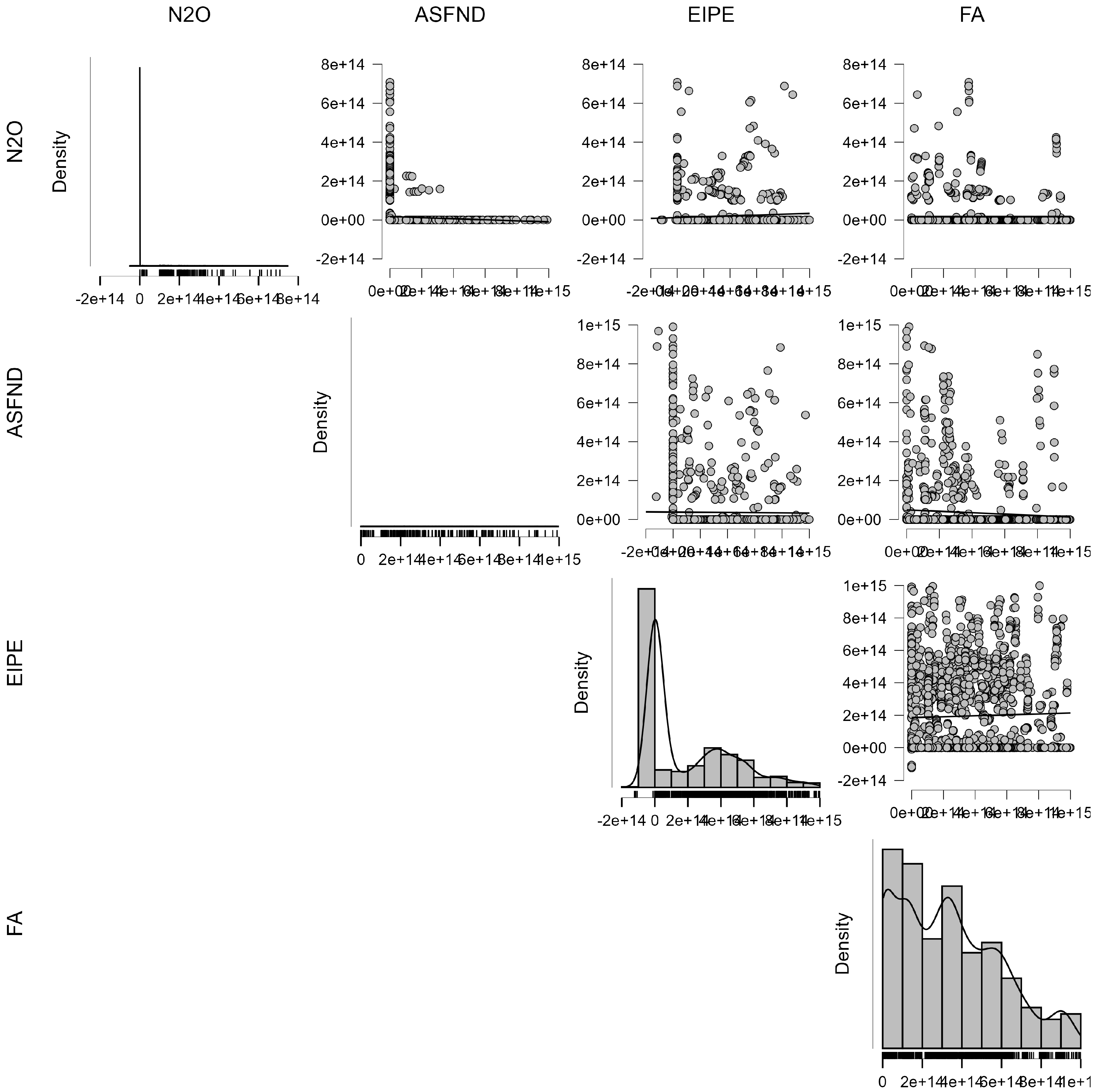
4.1.1. Clusterization Model for the Estimation of the E-Environmental Component Within the ESG Model

In the following analysis, we compare four different machine learning algorithms applied to clustering, namely density-based, fuzzy c-means, hierarchical clustering, and neighborhood-based. The algorithms are analyzed through the use of a set of statistical indicators, namely the maximum diameter, minimum separation, Pearson’s γ, Dunn index, entropy, and Calinski–Harabasz index. The results are shown in the following table (Table 4).
In order to be able to make a comparison between the algorithms based on the identified indicators, it is necessary to proceed with the normalization as indicated in the following Table 5.
In selecting the most appropriate clustering algorithm out of a list of available algorithms, it is convenient to have a clear and systematic decision rule based on given performance measures. In the current instance, the algorithms were compared using a list of standard criteria, viz. maximum diameter, minimum separation, Pearson’s γ, Dunn index, entropy, and Calinski–Harabasz index. In order to make the decision-making process as objective as possible, one useful approach is to tally the number of measures on which each algorithm performs best. On the basis of this rule, the density-based algorithm is the best option, with optimum performance on several key measures such as maximum diameter, minimum separation, and Dunn index. The second best option is the neighborhood-based algorithm, with its best performances in entropy and Calinski–Harabasz indices. In turn, the hierarchical algorithm performs best in terms of Pearson’s γ but without comparable performance in other key measures. On the other hand, the fuzzy c-means algorithm exhibits uniformly poor performance across all measures with the best performance of intermediate scores and without leading in any specific category. In instances wherein a tie between algorithms is observed, one possible alternative approach is to calculate the average normalized scores on all measures and then select the algorithm with the highest overall average. Such an approach assures comprehensive and balanced evaluation by taking into account at the same time cluster compactness, cluster separation, internal cohesion, and overall quality of clustering. In the current analysis, however, there was no tie and thus the simpler approach of tallying “best-performing” measures sufficed in the selection of an algorithm. In conclusion, the application of this simple yet effective decision rule enables one to effortlessly and accurately decide on the most suitable clustering algorithm [78,79,80]. Thus, for the setting being examined, the density-based algorithm is by far the preferable alternative due to its general high performance across a set of important evaluation metrics, thereby being the most stable clustering algorithm among the ones being investigated (Figure 2).
The clustering outcome presents a highly unbalanced clustering structure with a single large cluster (Cluster 1) containing the vast majority of data points and a very small second cluster (Cluster 2). There are eight noise points, suggesting that a small portion of the dataset was not assigned to a cluster, most likely due to outliers or datapoints very poorly represented by the uncovered clusters. Cluster 1, containing 1912 points, explains almost all of the within-cluster heterogeneity (99.6%) and has an extremely high sum of squares (6,575,671), suggesting that the cluster is capturing most of the variance in the data and either reflects a naturally compact and well-defined structure or potential over-grouping through an overly inclusive cluster assignment. Cluster 2, in contrast, contains only 10 points and explains a negligible proportion of the explained within-cluster heterogeneity (0.4%). Its internal sum of squares (29.027) is substantially lower than that of Cluster 1, as would be anticipated from the cluster’s size. However, that its silhouette score is comparatively lower (0.465 versus 0.646 for Cluster 1) suggests that Cluster 2’s cohesion and separation are lower, and it may have less distinct boundaries from points in its immediate neighborhood. The silhouette scores also support the assessment of clustering quality. Cluster 1 has a moderately high silhouette score (0.646), suggesting that points within this cluster are well separated from other clusters and internally cohesive. Cluster 2 also possesses a lower silhouette coefficient (0.465), indicating its members are less well defined, perhaps overlapping with the large Cluster 1. Overall, the clustering solution is dominated by the size of Cluster 1. This skewness may either indicate the necessity to tweak clustering parameters in an attempt to reveal a more substantively interesting split in the data or that the dataset itself simply has a highly skewed distribution with most points being part of a single dominant cluster [81,82,83]. Further investigation of clustering criteria and potential modification of distance measures or parameter adjustment may be warranted to enhance cluster discrimination (Figure 3).
The cluster means table explains the character of the three clusters by four environmental and economic measures: adjusted savings from net forest depletion, energy intensity level of primary energy, forest area percentage of land area, and nitrous oxide emissions in metric tons of CO2 equivalent per capita. The cluster pattern shows distinct grouping across the variables. Cluster 0 has both the highest adjusted savings at 0.847 and energy intensity at 1.801, suggesting that units or regions belonging to this cluster have high forest depletion but higher energy intensity. The negative forest area at −0.288 suggests lower forest cover, but nitrous oxide emissions at 5.586 are moderately high among the three clusters. This suggests that Cluster 0 potentially represents regions of higher industrialization and energy consumption but at high environmental expense. Cluster 1 is near zero for all the indicators, with adjusted savings, energy intensity, and nitrous oxide emissions near zero and forest area mildly positive at 0.003, suggesting some balance between environment and economic activity. This cluster most likely represents regions of sustainable utilization of resources or environmental–economic equilibrium. Cluster 2 is moderately high in adjusted savings at 0.606 but has the lowest energy intensity at −0.126, suggesting lower consumption of energy per unit of GDP. However, it also shares the same negative forest area proportion of −0.288 with Cluster 0, suggesting forest depletion. Its nitrous oxide emissions at 8.886 are the highest, suggesting very high emissions despite moderately lower energy intensity. This cluster can lead us to areas of high environmental degradation in the form of emissions, maybe from agriculture or other non-energy sectors. In total, the clusters differ by environmental impact and energy use. Cluster 0 is energy-intensive with medium emissions, Cluster 1 is balanced, and Cluster 2 has a lower energy intensity but with the highest emissions [84,85,86].

4.1.2. ML Regressions for the Estimation of the E-Environmental Component Within the ESG Model

In order to determine the most suitable algorithm, a comparison of the most significant performance measures such as mean squared error, root mean squared error, mean absolute error, and the coefficient of determination is needed. The best model must have the lowest mean squared error, root mean squared error, and mean absolute error and the highest coefficient of determination, which indicates the level of variance in the data explained by the model. K-nearest neighbors among all the algorithms has the highest value of the coefficient of determination of 0.182, explaining the most variance in the data. Although it does not have the lowest mean squared error or root mean squared error, the fact that it is capable of capturing the underlying patterns of the data better than the other algorithms makes it the most suitable algorithm. Other models, including random forest and decision tree, are also very good even though they have relatively lower values of the coefficient of determination. Models like boosting regression, support vector machine, and regularized linear regression have no explanatory power with very low values of the coefficient of determination and hence are not suitable [87,88,89]. Based on the trade-off between explanatory power and error measures, k-nearest neighbors is the best among the compared models (Table 6).
The relative importance of the variables in predicting nitrous oxide emissions in metric tons of CO2 equivalent per capita is represented by the mean dropout loss values of k-nearest neighbors. Larger dropout loss values mean that the removal of a variable results in a large increase in model error, proving it to have a strong contribution to prediction. The results show that forest area as percentage of land area has the largest mean dropout loss at 7.852 × 10¹³ and is thus the most important factor in nitrous oxide emissions prediction. This would imply that regions with extreme changes in forest cover most likely witness high variations in emissions, which may be due to deforestation, land use change, or losses in carbon sequestration. The second largest mean dropout loss of 7.106 × 10¹³ is contributed by the energy intensity level of primary energy, meaning that it also has a large role in emissions prediction. This is a manifestation of the strong relationship between energy consumption per unit of GDP and nitrous oxide emissions because a higher energy intensity level comes with increased reliance on fossil fuels, inefficient energy use, and higher greenhouse gas emissions. The adjusted savings from net forest depletion has the smallest mean dropout loss at 5.738 × 10¹³, meaning that while it is still a significant factor in emissions prediction, its effect is not as strong as those of forest area and energy intensity. This could mean that while net forest depletion influences changes in emissions, its effect is more indirect or contingent on other economic and environmental processes. Collectively, these results suggest that forest cover is the strongest predictor of nitrous oxide emissions, closely followed by energy intensity, with proportionally less contribution from net forest depletion [89,90,91]. The k-nearest neighbors model thus relies strongly on forest cover and energy efficiency in its emissions prediction, echoing the part of land use policy and energy use strategy in managing nitrous oxide emissions (Table 7).
The provided data include additive explanations for predictions of nitrous oxide emissions in units of metric tons of CO2 equivalent per capita, from three predictor variables: adjusted savings from net forest depletion, energy intensity level of primary energy, and forest area percentage of land area. The base value is the same for all cases at about 1.496 × 10¹³, and it represents the common starting point for predictions before the contributions from the variables alter it. The predicted values are highly variable for cases, as a result of the combined influence of the predictor variables. Case 1 has a relatively low predicted value of 0.382. The contributions show a very large positive effect of adjusted savings at 54.646 but strong negative effects from energy intensity at −3.752 × 10¹² and forest area at −1.121 × 10¹³. The enormous negative contribution of forest area shows that larger forest coverage is associated with lower nitrous oxide emissions. Case 2 has a very high predicted value of 2.575 × 10¹³, driven to a large degree by a very strong positive contribution from energy intensity at 2.152 × 10¹³. This shows that higher energy intensity is a key contributor to high nitrous oxide emissions for this case. Adjusted savings and forest area contributions are modest in comparison. Cases 3, 4, and 5 all have the same predicted value of 0.041. They are characterized by modest positive contributions from adjusted savings at 1.227 × 10¹² and large negative contributions from energy intensity at −6.127 × 10¹² and forest area at −1.006 × 10¹³. These cases show that lower energy intensity and larger forest area significantly reduce nitrous oxide emissions. Overall, the results identify energy intensity as a primary cause of increasing nitrous oxide emissions, with an ameliorating effect of forest area. Scenarios with high energy intensity contributions have higher emissions, and those with strongly negative forest area contributions have lower emissions [92,93]. This suggests that policies of energy intensity capping and forest area conservation or expansion can be effective options for nitrous oxide emission management (Table 8).

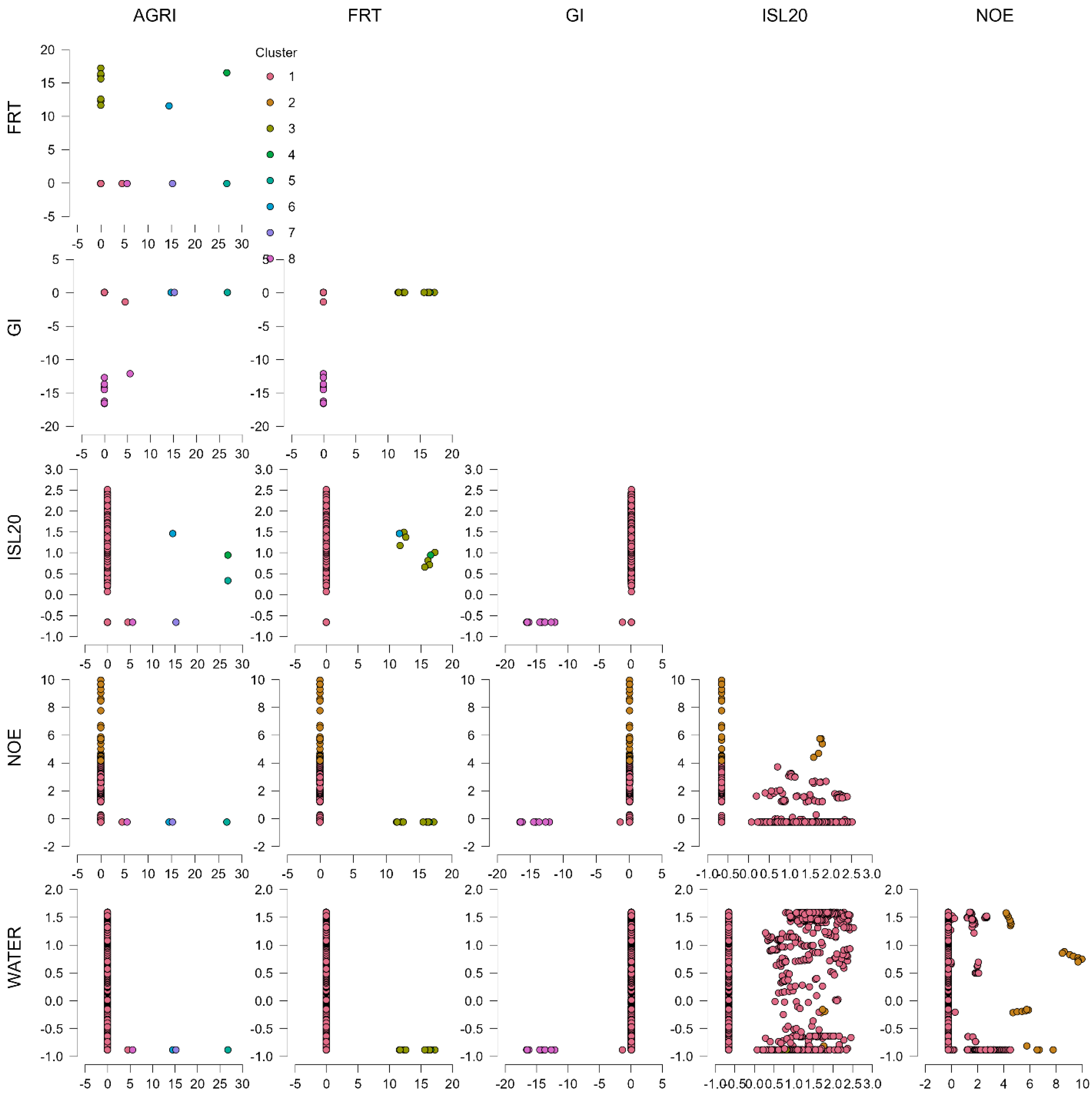
4.2. S—Social Econometric Results

In the following analysis we consider the relationship between NOE and some variables related to the social component in the ESG model. Specifically, we used panel data with fixed and random effects to estimate the following equation:
N O E i t = α + β 1 A G R I i t + β 2 F R T i t + β 3 G I i t + β 4 I S L 20 i t + β 5 W A T E R i t
where i = 193 and t = [2011;2020] (Table 9).
The positive relationship between nitrous oxide emissions and annualized average growth rate in per capita real survey mean consumption or income compared to the total population. The positive relationship between nitrous oxide (N2O) emissions, in per capita metric tons of CO2 equivalent, and the annualized average growth rate in per capita real survey mean consumption or income shows that income and consumption growth are linked with rising emissions of this potent greenhouse gas. Nitrous oxide, whose principal sources are agriculture, industry, and fossil fuel combustion, is a key cause of global warming owing to its lengthy atmospheric lifetime and large global warming potential. As incomes rise and economies grow, increased agricultural activity—particularly through the use of nitrogen-based fertilizers—leads to higher N2O emissions. Industrial growth and increased energy consumption also increase emissions. The trend is a textbook environmental–economic trade-off where economic development is obtained at the cost of environmental loss. The correlation suggests the implementation of sustainable development policies, for instance, encouraging efficient fertilizer use, investing in clean technologies, and implementing carbon pricing mechanisms to limit emissions without choking growth. Policymakers must balance economic objectives and environmental protection, ensuring development pathways include green growth initiatives. In the absence of early action, climate change may be driven by future income growth, so there is a need to integrate sustainability into economic planning [94,95,96].
The positive relationship between nitrous oxide emissions and fertility rate in terms of total births per woman. The positive relationship between nitrous oxide (N2O) emissions, in metric tons of CO2 equivalent per capita, and fertility rate, in total births per woman, means that rising birth rates are accompanied by rising emissions of this potent greenhouse gas. The relationship is explained by a group of socioeconomic and environmental determinants. In highly fertile countries, a rising population causes rising demand for food production, particularly in agriculture, which is the overwhelming source of N2O emissions. The widespread use of nitrogen-based fertilizers and livestock farming releases tremendous amounts of nitrous oxide to the environment. Additionally, greater population growth increases energy consumption, land use change, and deforestation, all of which contribute to high emissions. The relationship reflects the challenge of reconciling population growth with environmental sustainability. Highly fertile nations face pressures to boost agricultural and industrial production to feed and serve their populations, which entails high greenhouse gas emissions. Policy responses to this challenge include measures to promote sustainable agriculture, increased family planning activities, and investment in clean energy technologies. By integrating environmental concerns within population and economic policies, societies can attempt to curtail emissions while encouraging long-term sustainable development [97,98,99].
The negative relationship between nitrous oxide emissions and the Gini index. The inverse relation between nitrous oxide (N2O) emissions, in metric tons of CO2 equivalent per capita, and the Gini index demonstrates that with decreasing income inequality, N2O emissions per capita rise. The Gini index quantifies income inequality on a scale from 0 (perfect equality) to 100 (perfect inequality), and lower values represent more equitable income distribution. One explanation for this relationship is that countries with lower income inequality have greater overall economic progress, which is coupled with greater industrialization, energy consumption, and intensification of agriculture—all prominent sources of N2O emissions. More equitable income distribution can translate to greater access to modern infrastructure, greater consumption levels, and greater agricultural production to meet the needs of a larger middle class. These processes result in greater emissions from fertilizer use, livestock production, and the burning of fossil fuels. Countries with high income inequality, however, have more poor people and thus lower per capita emissions due to low industrial and agricultural activity. This is a characteristic of the complex trade-off between economic equity and environmental sustainability. Policymakers must design policies to achieve both economic inclusivity and sustainable development, including investment in clean technologies and environmentally friendly agricultural production systems [100,101,102].
The positive relationship between nitrous oxide emissions and income share held by the lowest 20%. The positive relationship between nitrous oxide (N2O) emissions, in metric tons of CO2 equivalent per capita, and the share of income held by the lowest 20% suggests that as income becomes more equally distributed, per capita N2O emissions rise. This is understandable given the broader economic growth and increased consumption patterns that follow more equal income distribution. When the lowest 20% of the population hold a high proportion of national income, this is usually a sign of reducing poverty and greater access to resources, including food, energy, and modern infrastructure. As poorer segments of society increase in economic standing, their consumption of goods and services rises, inducing greater agricultural activity, industrialization, and consumption of energy—all direct sources of nitrous oxide emissions. For instance, greater fertilizer use in agriculture, expanded livestock farming, and greater use of fossil fuels for transportation and energy consumption all lead to greater emissions. This correlation poses a challenge to balancing economic inclusivity and environmental sustainability. While reducing income inequality buttresses social and economic stability, it seems to lead to greater greenhouse gas emissions. Sustainable initiatives, including investments in clean energy and efficient agricultural technology, are necessary to offset environmental impacts while promoting equitable growth [103,104,105].
The negative relationship between nitrous oxide emissions and people using safely managed drinking water services. The inverse relation between nitrous oxide emissions, in metric tons of CO2 equivalent per capita, and the percentage of the population with access to safely managed drinking water services illustrates that access to clean water increases while per capita N2O emissions fall. The relation encapsulates general trends of socio-economic progress, environmental governance, and agricultural efficiency. Countries with widespread access to safely managed drinking water would be those that have well-developed infrastructure, better management of resources, and greater environmental protection. Such factors work in synergy with each other to suppress nitrous oxide emissions by promoting sustainable agricultural practices, cutting down the application of nitrogenous fertilizers, and enhancing wastewater treatment processes. Efficient water management can also limit nitrogen leaching from agriculture, a major source of N2O emissions. Secondly, nations with better water services would be likely to implement environmental policies that minimize greenhouse gas emissions without undermining economic growth. At the other end, regions with low access to clean water would be likely to have weak environmental protection and inefficient agricultural systems that lead to high per capita emissions. The absence of wastewater treatment and excess application of fertilizers lead to nitrogen accumulation in water bodies, indirectly increasing nitrous oxide emissions. The issue must be resolved by concerted policies that promote environmental sustainability as well as public health, such that gains in infrastructure are translated into greenhouse gas emission savings [106,107,108].

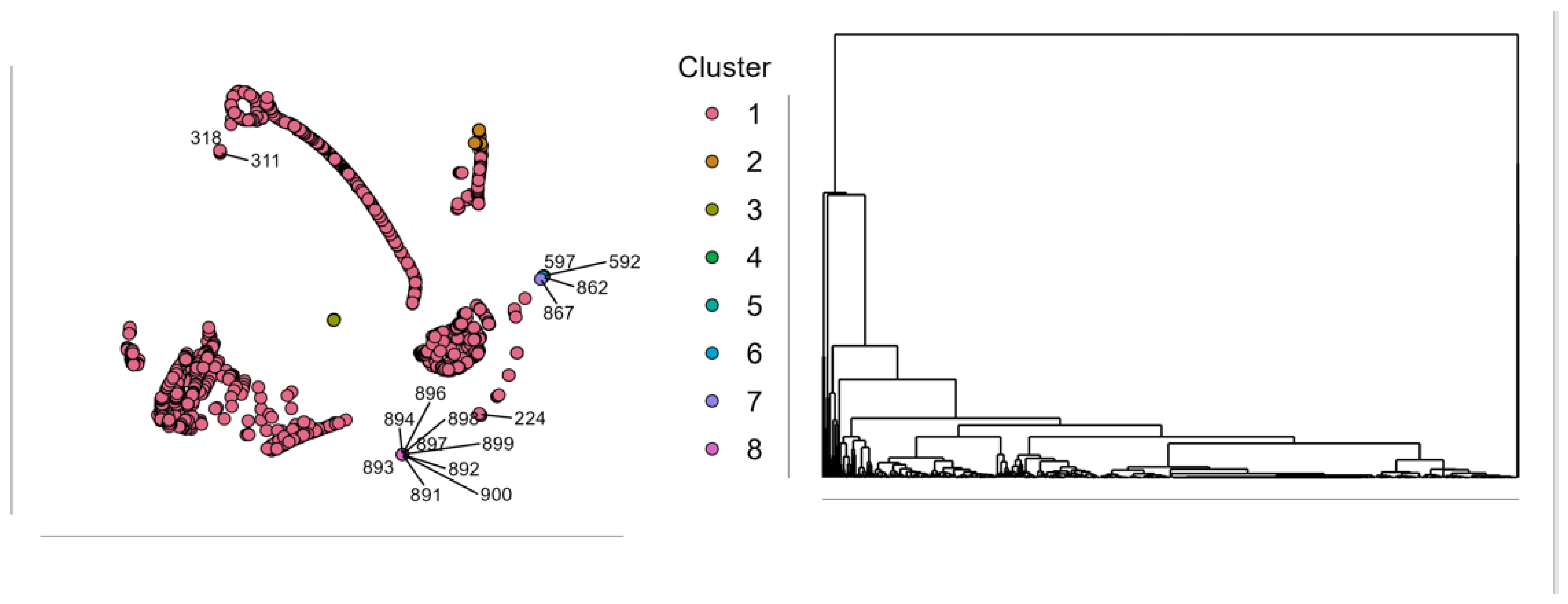
4.2.1. Clusterization Model for the Estimation of the S-Social Component Within the ESG Model

In the following analysis, we compare four different machine learning algorithms applied to clustering, namely density-based, fuzzy c-means, hierarchical clustering, and neighborhood-based. The algorithms are analyzed through the use of a set of statistical indicators, namely the maximum diameter, minimum separation, Pearson’s γ, Dunn index, entropy, and Calinski–Harabasz index. The normalized results are shown in the following table (Table 10).
Hierarchical clustering is the top-performing algorithm on the raw data due to its best performance on a number of key clustering evaluation measures. It has the lowest maximum diameter, indicating clusters created by this algorithm are more compact and well defined. It also has the highest minimum separation, and the clusters are well separated from one another, a key consideration while evaluating the quality of a clustering algorithm. Furthermore, hierarchical clustering is the top-performing algorithm among the algorithms on the Dunn index as well as the Calinski–Harabasz index. The Dunn index, a measure of the ratio of minimum inter-cluster distance to maximum intra-cluster distance, is much higher with hierarchical clustering than with the other algorithms. A higher Dunn index corroborates the fact that the clusters are not only well-separated but also compact, corroborating the observation that hierarchical clustering is the best algorithm. Similarly, the Calinski–Harabasz index, a measure of cluster validity that compares dispersion between the clusters to dispersion within the clusters, is highest with hierarchical clustering, providing further support to hierarchical clustering’s tendency to create high-quality clusters. The application of normalization techniques, i.e., Z-score normalization and Min-Max normalization, was uninformative to the algorithm selection process due to inherent effects on the data. Z-score normalization standardizes each feature by centering it around a mean of zero and scaling it based on its standard deviation. While the process ensures that all features have an equal contribution, it has the effect of nullifying useful differences between clustering algorithms in this dataset. The values became almost identical after standardization, and it was impossible to differentiate between different algorithms based on their performance. Similarly, Min-Max normalization transforms all values into a defined range, most typically zero to one. This is particularly useful for preserving relative differences among data points but has disproportional effects for features with extremely extreme values. In these data, some measures such as the Calinski–Harabasz index had considerably larger magnitudes than others. Therefore, Min-Max normalization compressed the variance among measures and did not permit an equal comparison across clustering methods. In light of these limitations, the best approach was to utilize the raw, unnormalized data, where the hierarchical clustering method performed consistently better on valuable evaluation measures [109,110,111]. This approach guarantees that the selection of the optimal clustering method is performed on the basis of interpretable, substantive distinctions and not normalization method artifacts (Table 11).
The outcome of hierarchical clustering is an extremely unbalanced cluster distribution, with a single large cluster containing 1884 data points and the remaining clusters being extremely small, with many single-member clusters. This would suggest that the data have unbelievably strong central grouping tendencies, with very few outliers or extremely dissimilar observations that have been isolated by the clustering algorithm into their own individual clusters. We see this evidence borne out again with the proportion of within-cluster heterogeneity explained. The largest cluster accounts for 95.1% of the within-cluster variance, suggesting that an overwhelming majority of data points are of similar nature. Contrastingly, however, the smaller clusters account for infinitesimal proportions of within-cluster heterogeneity, with values as low as 0.000, suggesting that these are perhaps best conceived of as extreme cases or anomalies rather than meaningful clusters. The within-cluster sum of squares relates much the same story, with the largest cluster accounting for the vast majority of overall variance (4,509,331), while the single-member clusters have within-cluster sums of squares of 0. This would suggest that these clusters consist of entirely unique observations that do not share any features with any other data points. The silhouette scores continue to support this finding, as a majority of the clusters have high values, suggesting well-separated and compact clusters. However, the single-member clusters take a silhouette value of zero, which suggests these points do not fall naturally into any inherent cluster structure within the data. Looking at the overall cluster structure, the between-cluster sum of squares of the model is equal to 6830.97, while the total sum of squares is equal to 11,574. This would indicate that the cluster model explains much of the overall variance with a well-defined group separation. However, the presence of many single-member clusters is concerning from the perspective of clustering granularity correctness [81,82,83]. This is more indicative of data with a strong central tendency and some aberrant observations rather than many equally significant clusters (Table 12).
The trends of the clusters from the hierarchical clustering are each unique in the trends of the emissions of nitrous oxide, with the environmental effect varying considerably among the clusters. Cluster 2 has the only significantly positive emission of nitrous oxide (6.491 metric tons of CO2 equivalent per capita), while the rest of the clusters are negative, with most of the clusters having the same value of approximately −0.240. This shows that Cluster 2 is a unique sub-set of the observations with significantly higher emissions of greenhouse gases compared to the other clusters. A closer look at the socio-economic variables of Cluster 2 reveals that it does not include extreme deviations in the annualized growth rate, fertility rate, or the Gini index. However, the income to the lowest 20% is negative, showing higher inequality in the distribution of wealth compared to some of the other clusters [112]. The population with access to safely managed drinking water services is also relatively higher at 0.428%, showing that this cluster may consist of countries or regions with advanced infrastructure but with higher emissions (Figure 4).
Clusters 3, 4, 5, 6, 7, and 8, which have similar levels of emission of nitrous oxide at −0.240, differ significantly in the other factors. Specifically, Clusters 3 and 4 both possess high levels of fertility (14.549 and 16.532, respectively) and high positive levels of the growth rate per year, making these distinct from the other clusters. These clusters would then represent developing economies with high population growth but comparatively modest per capita emissions. Clusters 5, 6, and 7 differ in economic growth rates and the income share of the poorest 20% but are similar in the levels of emission of nitrous oxide, which means that the levels of emissions of these clusters are not strongly correlated with economic performance and income distribution. Cluster 1 is of special note with its moderately lower level of emission of nitrous oxide (−0.087), unlike the other clusters that possess the common value of −0.240. This slight deviation could represent slightly differing economic or industry structure within this cluster, but the difference is not as significant as that of Cluster 2 [112]. The clustering results suggest that emissions of nitrous oxide are not strongly correlated with all socio-economic factors but that Cluster 2 is the only one with the highest emissions and relatively moderate economic and social attributes (Figure 5).

4.2.2. ML Regressions for the Estimation of the S-Social Component Within the ESG Model
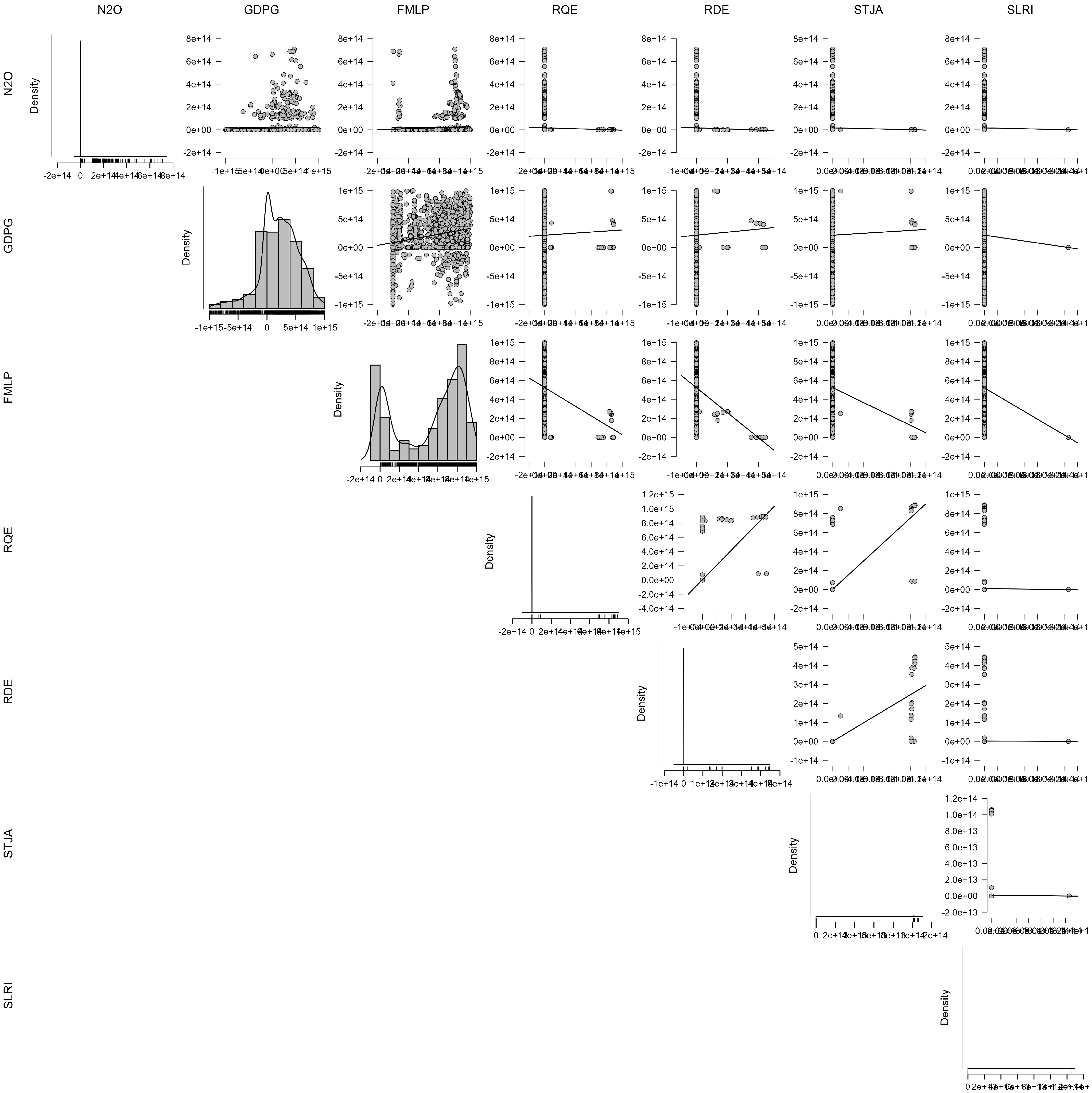
The process of normalization was applied to ensure that all performance metrics were on a comparable scale, allowing for an unbiased evaluation of the different machine learning algorithms. Min-Max normalization was chosen as it transforms values into a fixed range between zero and one, preserving the relative differences among data points while ensuring that no single metric dominates the analysis due to differences in magnitude (Table 13).
We compare the performance of the algorithms using the following statistics: mean squared error, root mean squared error, mean absolute error, and R2 score. Normalization of the measures eliminated the effect of large-scale numbers such as the ones used with MSE so that the relative performance of each model could sensibly be compared. Choosing the best model depended on multi-criteria evaluation since the best model would minimize error measures while maximizing the measure of predictability as given by the R2 score. The best model was the random forest model since it had the lowest root mean squared error and the highest R2 score that shows that it has the most accurate forecasts while explaining the largest amount of variance in the data. Decision tree performed fairly on mean squared error but had poor generalization. Boosting was another contender since it had the lowest mean absolute error that shows that it makes fewer errors per case on average but had the lowest R2 score that shows poor predictability [113]. The process of normalization helped to bring out these trade-offs so that model choice would not be influenced by the raw measure’s scale but would instead depend on the balanced consideration of multiple performance measures (Table 14).
The relative importance of the features indicates that the most important predictor of the emissions of nitrous oxide is the proportion of individuals with safely managed drinking water services, with a relative importance of 52.228. This indicates high correlation of the use of safely managed drinking water services with variation in the emissions of nitrous oxide, and this may indicate variations in levels of infrastructure, of industry, or of environment policy between regions. The fertility rate, with a relative importance of 36.154, is also of high importance as a predictor and indicates that population matters are of greatest importance in emission trends, perhaps as determinants of resource use and of agricultural output. The share of income of the poorest 20% and the Gini index, with a relative importance of 7.708 and 3.854, respectively, indicate that economic inequality plays no important role in emissions, perhaps associated with unequal use of industry and of energy. Average growth in per capita real survey mean consumption or income on the basis of per annum seems to influence the emissions hardly at all, with a relative importance of 0.057, and indicates that variation in economic growth over the short term influences the emissions of nitrous oxide in the dataset at hand hardly at all. Mean dropout loss calculated as the root mean squared error over 50 permutations is relatively stable across the variables and indicates that observed importance rankings are not perturbed by random resampling [114,115]. They emphasize the necessity to carry out additional research on the role of population trends and infrastructure on the trends of emissions of nitrous oxide and the policy implications of expanding the coverage of basic services as a means of mitigating the environmental impacts (Figure 6).
The additive explanations of the predictions in the test set reveal the relative importance of each of the features to the estimated nitrous oxide emissions. The baseline value, the prediction in the absence of the specific feature contributions, is high and uniform across cases and reveals that the underlying model estimates high levels of emissions even in the absence of explanatory factors. The feature contributions highlight that the most important factor in the determination of the predicted values is the coverage of people served with safely managed drinking water services. In Cases 3, 4, and 5, this variable has positive contributions to the prediction with the highest of 3.536 × 10,133.536\times 1013, indicating that higher coverage of the managed drinking water services is associated with higher emissions that are predicted. However, in Cases 1 and 2, this feature has negative effect and lowers the predicted emissions by up to 2.320 × 10,122.320\times 1012, which indicates that its effect is not uniform across instances. The fertility rate, number of births per woman, and income proportion owned by the lowest 20% appear to have no quantifiable influence on the predicted values since their contributions are uniform at zero, indicating that the variables are not drivers of the emissions of the nitrous oxide in the test set. The Gini index of income inequality has high negative contributions in Cases 3, 4, and 5, with the highest being −4.869 × 10¹³–4.869\times 1013, indicating that higher inequality is associated with lower emissions in the particular cases. The negative relationship may indicate that in the areas of higher income inequality, the emissions are concentrated in specific economic sectors and not distributed evenly among the population. By way of contrast, in Cases 1 and 2, the Gini index contributes positively but with lower magnitude to the forecasted values and so supports the hypothesis that its influence is conditional on the underlying socio-economic conditions. The average per capita real survey mean consumption or income’s growth rate per annum does not make significant contributions to the forecasted values in either of the cases and so does not play an important role in explaining the levels of nitrous oxide emissions in this dataset. Having large positive and negative feature contributions in each of the cases suggests that the relationship among the predictors of the levels of nitrous oxide emissions is strongly conditional on the circumstances. Further studies on interaction effects among variables are required to fully reveal the mechanisms behind the levels of emissions. The results also suggest the need to exercise caution in interpreting policies since the same feature may yield contrasting effects in different regions or economic circumstances (Table 15).

4.3. G—Governance

In the following analysis, we consider the relationship between NOE and some variables related to the governance component in the ESG model. Specifically, we used panel data with fixed and random effects to estimate the following equation:
N O E i t = α + β 1 G D P G i t + β 2 F M L P i t + β 3 R Q E i t + β 4 R D E i t + β 5 S T J A i t + β 6 S L R I i t
where i = 193 and t = [2011;2020] (Table 16).
The positive relationship between nitrous oxide emissions and GDP growth. The positive relationship between the emissions of nitrous oxide in metric tons of CO2 equivalent per capita and the increase in the GDP shows that the emission of N2O increases as the economies expand. Industrial, agricultural, and energy-demanding activities that induce economic growth are also responsible for high emissions of greenhouse gases. Increased economic growth is generally associated with high industry production, high consumption of energy, and high agricultural production that are among the highest contributors to emissions of nitrous oxide. Most developing and emerging economies achieve economic growth through industries that include manufacturing, transport, and large-scale agriculture that rely on high applications of nitrogen-based fertilizers and fossil fuels. Increased agricultural production to meet growing food demands further results in higher emissions from soil management and livestock production. While economic growth raises living standards and lowers levels of poverty, it poses the challenge of emission control. Most high-growth economies struggle to reconcile economic growth with measures of sustainability. Solving this challenge requires investment in clean technologies, efficiency in the use of energy, and sustainable agriculture to decouple economic growth from the degradation of the environment. Economic policies in the long term should include measures of sustainability to guarantee that economic growth does not result in higher levels of emissions of greenhouse gases [95,96,116].
The negative relationship between nitrous oxide emissions and the ratio of the female to male labor force participation rates. The negative relationship between the per capita emissions of nitrous oxide in metric tons of CO2 equivalent and the female-to-male ratio of the workforce means that per capita emissions of N2O decline as the workforce becomes increasingly balanced between the two genders. This is representative of deeper economic and social transformations that include the structure of the workforce, the application of industries, and the environmental policies. Economies with higher workforce participation of females experience the transition of high-emission industries such as agriculture and heavy industry to service and knowledge economies. An increasingly balanced workforce is generally typified by economic diversification, increased investment in human capital in the form of education, and the application of more sustainable development policies that result in lower per capita emissions of nitrous oxide. Increased participation of females in the workforce is also associated with progressive policies on the protection of the environment, resource efficiency, and sustainable agriculture that result in lower emissions. Economies with lower workforce participation of females apply more traditional methods of agriculture that are high-emission sources of N2O through the application of high amounts of fertilizer and cattle rearing. These economies apply less stringent policies on the environment and fewer opportunities to apply cleaner technologies. Gender equality in the workforce not only results in higher economic growth and social development but also in the environment’s sustainability through the encouragement of lower-emission economic activities [117,118,119].
The positive relationship between nitrous oxide emissions and estimated regulatory quality. World Bank data from 2020 show that several nations with strong regulatory quality—including New Zealand (2.93 tCO2e/capita), Australia (1.92), Ireland (1.92), Canada (1.24), and Finland (1.06)—also report some of the highest per capita nitrous oxide (N2O) emissions worldwide. Stronger governance and regulatory systems are usually linked with more efficient environmental protection; thus, this favorable link seems contradictory. But, when one takes into account the larger background of industrial structure and economic growth, the link becomes more obvious. High-regulatory-quality countries usually have well defined legal institutions, administrative efficiency, and strong policy implementation tools. These qualities support large-scale agricultural development—sectors that are main sources of N2O emissions—industrial modernization, economic expansion, and others. Particularly, nations like New Zealand and Ireland are quite dependent on fertilizer-intensive livestock farming, which greatly increases N2O emissions. So, good regulatory quality does not guarantee lower short-term emissions. Instead, it shows a state’s ability to develop industrially and economically—usually leading to more emissions during the expansion stage. On the other hand, future environmental control, sustainable development changes, and the incorporation of green technologies all depend on the same institutional power. Effective regulatory systems are more likely to put in place emissions monitoring, adopt mitigation policies, and harmonize national development with climate goals over time. Seen in this way, the reported favorable link could indicate a transition period in which regulatory capacity initially drives growth of emissions and later promotes long-term environmental control and sustainable development [120,121,122].
The positive relationship between nitrous oxide emissions and research and development expenditure. The positive relationship of the emissions of nitrous oxide in metric tons of CO2 equivalent per capita with the expenditure on research and development (R&D) as a percentage of the GDP shows that economies that spend more on research and development experience higher per capita emissions of N2O. This is so because the interlinkage of technological advancement, industrialization, and increased agricultural and energy production is the source of the majority of the emissions of nitrous oxide. Economies that spend more of their GDP on R&D experience faster economic and industrial growth. Technological advancement stimulates efficiency and productivity but also tends to lead to increased emissions from industries such as manufacturing, transport, and large-scale agriculture. Greater expenditure on R&D tends to lead to the production of new fertilizers, better agricultural practices, and industrial processes that increase output but increase emissions of nitrous oxide. Economies driven by research also tend to utilize advanced infrastructure, high-energy industries, and higher consumption levels that continue to propel emissions growth. But in the long run, increased expenditure on R&D enables the production of cleaner technologies, more sustainable agricultural practices, and better use of energy. Although initial emissions rise with the expansion of industry, continued innovation enables the environment to adapt to the negative effects of emissions through the encouragement of sustainable substitutes and emission-reducing technologies [123].
The negative relationship between nitrous oxide emissions and scientific and technical journal articles. The negative relationship between the emissions of the gas nitrous oxide (N2O) and the quantity of scientific and technical publications suggests that higher research output is associated with lower per capita emissions. Scientific advancement generates green technologies, efficient agriculture, and cleaner industries that avoid the use of excess nitrogen. Good research institutions and policies of innovation result in green technologies, while evidence-based policymaking supports stricter emission controls. Lower research output inhibits technological advancement and leads to higher emissions. Similarly, the negative relationship of the emissions of N2O with the index measuring the quality of legal rights suggests that higher legal protection results in lower emissions. Clearly defined legal institutions make regulation more effective, facilitate green investment, and result in sustainable use of resources. Good legal institutions increase the quality of government and responsibility and result in effective control of pollution. Weak legal protection inhibits access to finance to achieve sustainable development and results in weak regulation and higher emissions. Strengthening scientific research and the quality of legal institutions is essential to lowering the emissions of N2O while maintaining economic and environmental stability [124,125].

4.3.1. Clusterization Model for the Estimation of the G-Governance Component Within the ESG Model

In the following analysis, we compare four different machine learning algorithms applied to clustering, namely density-based, fuzzy c-means, hierarchical clustering, and neighborhood-based. The algorithms are analyzed through the use of a set of statistical indicators, namely the maximum diameter, minimum separation, Pearson’s γ, Dunn index, entropy, and Calinski–Harabasz index. The normalized results are shown in the following table (Table 17).
The optimal clustering algorithm is determined from the normalized performance measures of the maximum diameter, minimum separation, Pearson’s γ, Dunn index, entropy, and Calinski–Harabasz index. The optimal algorithm should have a low maximum diameter to indicate that the clusters are compact, high minimum separation to indicate that the clusters are well separated, high Pearson’s γ to indicate good quality of the clusters, high Dunn index to indicate cluster compactness and separation, low entropy to indicate less randomness in cluster assignments, and high Calinski–Harabasz Index to measure the overall performance of the clusters. With the results normalized, the optimal algorithm is hierarchical clustering. Hierarchical clustering has the lowest maximum diameter to indicate that the clusters are compact and high minimum separation to indicate that the clusters are well separated. Hierarchical clustering also has a high Pearson’s γ to indicate strong cluster cohesion. Furthermore, its Dunn index is high among the algorithms to confirm that the clusters are both compact and well separated. Even though its entropy is higher than the best case but not the highest, it is within the threshold to indicate that the cluster structure is reliable. The Calinski–Harabasz Index is also high among the algorithms to confirm that the overall performance of the clusters is high. Even though neighborhood-based clustering has the highest Calinski–Harabasz index among the algorithms, it does not rank high in other critical measures like maximum diameter and minimum separation to make it less effective in providing the clusters to be both compact and well separated. Random forest has extreme readings on some of the measures, like very low minimum separation and a weak Pearson’s γ, to indicate that it does not produce clusters that are well defined. Density-based and fuzzy c-means clustering perform unevenly with both positive and negative sides to their performance in cluster separation and cohesion [126]. Based on these facts, hierarchical clustering is the most balanced and efficient algorithm to estimate the emissions of nitrous oxide so that the clusters are well separated and tight with high overall clustering structure (Table 18).
The results of hierarchical clustering indicate that the distribution of cluster sizes is highly imbalanced, with one large cluster of 1864 members and the remaining clusters of significantly fewer members, with several clusters having fewer than 10 members and one cluster containing 1 member. This suggests that the dataset is characterized by strong central grouping behavior with few outlying cases or highly dissimilar subgroups. The explained proportion of within-cluster heterogeneity supports this observation in the sense that Cluster 1 explains 97.7% of the overall within-cluster variation, further making it predominant. The small clusters make a negligible contribution to overall heterogeneity, with some being close to zero, particularly in Cluster 10, where the explained proportion is essentially zero. The within-cluster sum of squares is also similar in pattern, with the largest cluster making the largest single contribution to overall variance (4210.053) and the various small clusters having values close to zero, showing that these clusters are highly homogeneous or isolated cases. The silhouette scores also provide additional information on cluster quality, and most clusters have relatively high scores showing the clusters to be well separated and compact. Cluster 10 has the highest silhouette score of 1.000, and Cluster 8 has 0.000, showing poor separation and misclassification [127,128,129]. The overall model performance, as provided by the between-cluster sum of squares (9193.65) to the overall sum of squares (13,503), shows that the clustering structure captures the majority of the dataset’s variance and that it is partitioning the data meaningfully (Figure 7).
The clusters represent the interlinkages between economic, regulatory, and research-related factors of the emission of nitrous oxide. Cluster 8 has the highest average emissions of nitrous oxide (2.309), along with relatively high regulatory quality (4.690) and high research and development expenditure (9.960), showing that this cluster consists of economies that have high industrial or scientific activities that result in high emissions. Cluster 7 also has high emissions (0.830), along with high regulatory quality (5.621) and high research expenditure (9.926), showing that higher research intensity and stricter regulations are not necessarily associated with lower emissions but could instead relate to industrialized economies. Clusters 3 and 2 both have moderate emissions of nitrous oxide (0.318 and 0.300, respectively), with Cluster 3 characterized by high female-to-male participation in the workforce (9.127), possibly showing economies where the workforce is integrated along the lines of gender that influences the output of industries and the levels of emissions. Cluster 4 has the reverse pattern of high regulatory quality (14.445) and high research and development expenditure (10.327), with positive emissions of nitrous oxide (0.210), showing that even with high regulations and high research and development expenditure, emissions are moderate, possibly because of the presence of industries that use high amounts of energy. Clusters 6, 9, and 10 have the lowest emissions (−0.644), with Cluster 10 characterized by the highest number of scientific and technical articles published in journals (25.338), showing that high research output is responsible for lower emissions through the enhancement of technology and the application of better policies on the environment. Clusters 5 and 1 record near-zero emissions (−0.004 and −0.008, respectively), despite Cluster 5’s high quality of regulation (14.747) and moderate research expenditure (0.936), indicating that high regulations are not always effective in changing emissions in the absence of economic and industrial factors. The results show that high research expenditure and regulatory quality are not always effective in decreasing nitrous oxide emissions, as noted in Clusters 4, 7, and 8, where emissions are high despite high quality of government and scientific effort. Cluster 10, with high research output, and Clusters 6 and 9, with moderate research expenditure, indicate that scientific research could prove effective in decreasing emissions in the long run. The variations in emissions across clusters with the identical regulatory and research attributes indicate that the relationship between economic growth and industrial effort and the efficacy of the environment policy needs to be analyzed further to understand its role in emission trends (Table 19).

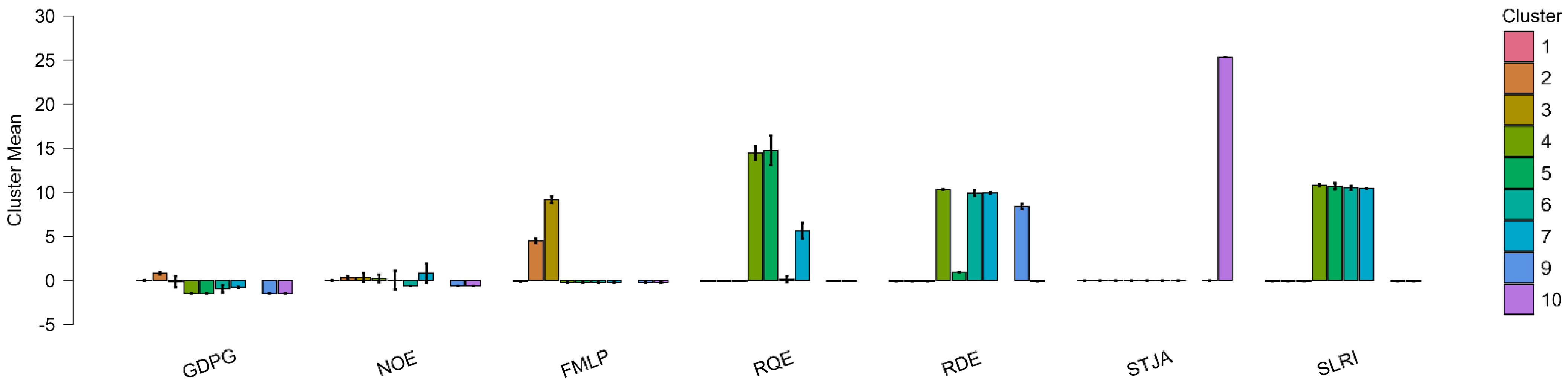
4.3.2. ML Regressions for the Estimation of the G-Governance Component Within the ESG Model

The selection of the best algorithm to predict the emissions of nitrous oxide is based on the evaluation of the normalized measures of error and explanatory power. The best model is the one that minimizes the error measures while maximizing the explanatory power of the model to the data variance. Random forest has the lowest normalized MSE (0.000), indicating the highest accuracy in the minimization of squared errors, while it also has the lowest scaled MSE (0.000), further indicating its superiority in error minimization. However, it has the largest RMSE (1.000), indicating its weakness in the measure of the root mean squared error. Decision tree has the lowest MAE (0.236), indicating that it makes the smallest average errors in the absolute sense, although it does not report the highest predictability. Random forest has the highest R2 score (1.000), indicating that it explains the largest proportion of the variance of the emissions of nitrous oxide. With this performance, the selection of random forest is the best overall since it achieves the best balance of minimum error and high explanatory power. Decision tree is the second since it has the lowest MAE, indicating the smallest errors per case, although it does not report the highest predictability. Boosting and K-nearest neighbors report moderate performance but fall behind the explanatory power of random forest [130,131]. The performance indicates that the application of random forest provides the highest predictability to predict the emissions of nitrous oxide (Table 20).
The significance of features indicates that regulatory quality, the female-to-male ratio of the workforce, and scientific research publications are the most significant predictors of the emissions of nitrous oxide. Regulatory quality has the highest mean decrease in accuracy (2.195 × 1027) and overall increase in node purity (6.433 × 1029), which indicates that regions with good regulatory institutions may experience high variations in emissions depending on the implementation of policies and green policies. The ratio of the workforce of females to that of males has the second largest mean decrease in accuracy (2.076 × 1027) and overall increase in node purity (5.768 × 1029), which indicates that dynamics among the two genders in the workforce may indirectly influence emissions, possibly through variations in the industries or economic development. Scientific and technical journal publications also emerge as the most significant factor with the highest mean decrease in accuracy (2.171 × 1027) and overall increase in node purity of 4.340 × 1029, which indicates that the intensity of research activities in science could be associated with technological development, green awareness, and green practices that affect emissions. Growth in the GDP has the smallest mean decrease in accuracy (3.630 × 1026) but is still significant in the trends of emissions and may represent the influence of the growth of industries and economic growth on the emissions of greenhouse gases. Expenditure on research and development as a fraction of the GDP is still significant but has the smallest overall increase in node purity of 1.891 × 1029, which indicates that its direct influence on the emissions of nitrous oxide is the weakest among features such as the quality of regulation and research output. Duplicate entries of scientific and technical journal publications may indicate that the processing of features is not consistent and needs to be verified to make sure that the variables are properly selected. The warning on the calculation of mean dropout loss shows that the application of the prediction function in the random forest model is in error. The error shows that dropout loss that is quantified in terms of RMSE could not be calculated and the ability to assess the unique predictive influence of each variable on the emission of nitrous oxide is limited. The limitation emphasizes the need to validate the results through other means to measure the features’ importance and the reliability of the results [132,133]. The results show that institutional factors, the workforce composition, and scientific developments are significant factors in the determination of the emission pattern and the need to incorporate policy interventions, gender-sensitive labor policies, and research expenditure to alleviate the environment’s challenges (Table 21).
The figures illustrate the relative importance of different predictors in estimating nitrous oxide emissions, using mean decrease in accuracy and total increase in node purity as measures of feature significance (Figure 8).
The first figure shows that the female-to-male labor force participation ratio (FMLP) has the largest decline in mean accuracy, i.e., that this factor is the most influential on model accuracy if omitted from the model, and that the relationship between gender dynamics in the labor market and emissions of nitrous oxide is strong. Scientific and technical journal articles (STJA) and regulatory quality (RQE) also see large declines in mean accuracy, i.e., research output and institutional quality are large determinants of variation in emissions. Research and development expenditure (RDE), the Strength of Legal Rights Index (SLRI), and growth in GDP (GDPG) see lower levels, i.e., that the effect on the accuracy of the predictions is comparatively small. The second figure, the overall increase in node purity, shows that regulatory quality (RQE) is the largest variable, i.e., high quality of regulation and institutional policies are the largest determinants of the emissions of nitrous oxide. The female to male ratio of the labor force (FMLP) is a close second, again affirming its role in determining emission trends. Scientific and technical journal articles (STJA) also see high levels of importance, perhaps reflecting the influence of technological advances and the transfer of knowledge to the environment. The growth in the GDP (GDPG) has more of an influence in this measure than in its influence on accuracy, i.e., economic growth is involved in emission trends but perhaps is more important in determining boundaries of decisions than in the accuracy of the model. The strength of legal rights (SLRI) and research and development expenditure (RDE) see comparatively lower overall increases in node purity, i.e., the provision of legal and finance support structures to enable the process of innovation and development is less important than more general institutional and labor market factors. The closeness of the relative significance of the three variables on the two measures suggests that emission trends are highly correlated with workforce structure, scientific progress, and regulatory frameworks. The lesser relative value of GDP growth suggests that short-term economic fluctuations may not be as important in determining emissions as structural factors such as workforce participation and the quality of governance. These findings emphasize the need for policy initiatives that integrate policies on the workforce, spending on research, and regulatory reforms in order to effectively address the environmental challenges of the emission of nitrous oxide [132].

5. Discussions of the Results and Innovativeness of the Contribution

Unpacking the complexity and multifaceted nature of the ESG framework in relation to nitrous oxide (N2O) emissions requires examining the effects of each ESG component separately: environmental, social, and governance. Different but connected systems of influence are encapsulated in each pillar. The biophysical pathways of N2O emissions are directly influenced by environmental factors, including energy intensity and forest depletion. Social indicators, such as fertility, income distribution, and access to essential services, are a reflection of economic and demographic forces that change emissions, land use, and consumption patterns. Institutional capacity to implement and enforce sustainability measures is determined by governance-related factors, including legal institutions and regulatory quality. The analysis enables a more accurate identification of the channels through which emissions are generated and managed by evaluating each component separately. Because it avoids confusing the distinct effects of variables that function on various levels—physical, social, and institutional—this decomposition is methodologically relevant. The foundation for creating an integrated framework that explicitly models the interplay between ESG dimensions is also laid by these deconstructed insights. Establishing the individual influence of each pillar, for example, is necessary to understand how strong governance can either moderate or amplify the environmental and social drivers of emissions. As a result, distinct analyses are essential for both analytical clarity and the development of a cohesive, systems-based ESG approach to emissions management and climate policy (Table 22).
The precise causal pathways that propel N2O emissions can be identified by dissecting the ESG model into its constituent parts. The foundation for a systemic integration, where the relationships between the environmental, social, and governance dimensions must be jointly modeled, is laid by this disaggregated analysis. A unified viewpoint is necessary for the efficacy of ESG policies since it becomes clear that strong governance can either mitigate or magnify the effects of environmental and social factors. The next critical step in tackling complicated environmental issues like nitrous oxide emissions on a global scale is to transition from a compartmentalized approach to an integrated and predictive ESG model.
This research provides a fresh and timely conceptual framework for assessing global N2O emissions using environmental, social, and governance (ESG) measures and thus responds to a significant research gap for sustainability studies and policy debate. Applying the reach of the models to N2O—a highly impactful greenhouse gas much too frequently ignored by existing approaches—the research extends the conventional, carbon-focused view of the impacts of climate within the analysis framework of the ESG to an integrated view of environmental responsibility.
Methodologically, this study stands out for utilizing the combination of panel econometric methods and advanced machine learning methods, such as clustering and prediction modeling. Not only do explanations grow more rich using the hybrid approach, but predictive power is significantly improved, which captures subtle, non-linear patterns that might go undetected using more traditional approaches.
A new innovation would be the creation of data-driven country typologies where countries would be categorized based on their emission pathways and performance regarding their environment, social, and governance factors. The categorization would provide evidence-based, nuanced observations for the creation of tailored policy interventions and for underpinning sustainable investing strategies.
By pointing to major structural drivers of N2O emissions—specifically forest cover and energy intensity—this research offers policymakers a more effective platform from which to embark upon focused activities to curb. Using macro-sustainability analysis and advanced data science, this research makes a valuable contribution to the literature by filling an important gap between climate and ESG interactions and offering policymakers sound evidence-driven avenues for more effective and equitable climate policy.

6. Limitations and Future Research

Though this research presents a unique combination of econometric and machine learning techniques to examine N2O emissions in an ESG framework, some shortcomings deserve attention. First, especially for developing nations with weaker statistical systems, the reliance on publicly available macro-level datasets, such as those from the World Bank, could raise questions about data completeness, granularity, and temporal consistency. These constraints could weaken the force of the conclusions reached and lower the accuracy of cross-country comparisons. Second, although the econometric models use fixed and random effects to compensate for unobserved heterogeneity, causal identification stays limited and possible endogeneity between ESG indicators and emission results cannot be completely excluded. Though the machine learning models show good predictive performance, they lack explanatory clarity since they do not reflect the structural causal mechanisms behind N2O emissions. Third, this study does not explicitly control for important structural country-level characteristics including geographic area, income group, or stage of economic development. Lacking such controls could create omitted variable bias and reduce the generalizability of the results across several socio-economic settings. Although the clustering algorithms generate country groupings that roughly correspond with development status, future work should improve robustness by adding stratified models or using macro-structural variables as controls.
Another drawback is the handling of ESG variables in isolation. Inherently multidimensional, the ESG framework comprises environmental, social, and governance pillars that sometimes interact synergistically or oppositely. Ignoring these interdependencies could cloud intricate mediating routes whereby ESG elements together affect emissions. Strong governance, for instance, could improve the implementation of environmental policies. Social inclusion could reduce the environmental effect of economic growth. Future studies should use structural equation modeling, interaction terms in fixed-effects regressions, or sophisticated machine learning architectures able to capture non-linear dependencies to explore such interaction effects. This would enhance the theoretical strength as well as the practical relevance of ESG-based emission modeling.
Important factors also relate to the clustering framework that is used. To capture the diversity and multidimensionality of ESG–emissions interactions across nations, this paper uses a comparative, multi-algorithm approach—testing density-based, fuzzy c-means, hierarchical, model-based, neighborhood-based, and random forest clustering techniques. A consistent set of internal validation metrics—silhouette scores, Calinski–Harabasz indices, Dunn indices, entropy, and Pearson’s γ—was used to assess every algorithm. Although this improves methodological openness, we acknowledge that certain algorithms, especially fuzzy c-means and neighborhood-based clustering, showed rather bad performance in terms of intra-cluster cohesion and separation. Low silhouette and Dunn values, as well as high entropy, suggest inaccurate cluster boundaries and potential data overlap, which undermine interpretability. By comparison, hierarchical clustering and density-based clustering revealed more obvious group structures and better validation results. A significant cluster size disparity still raises questions about overgeneralization and the representativeness of smaller clusters, particularly in the density-based model. Data-driven concentration or poor hyperparameter choice—for example, epsilon or minPts in DBSCAN—could cause this imbalance. Future research should include more robustness tests—sensitivity analysis across parameter settings, changes in distance metrics, and maybe ensemble clustering techniques—to enhance the interpretability and generalizability of the findings. Furthermore, including external validation using regional or income classifications and using sophisticated visualization tools could improve the clarity of clustering results and their applicability for policy creation.
Future studies could eventually gain from including subnational or firm-level ESG data to more precisely reflect emissions behavior at smaller spatial or organizational levels. Using hybrid causal inference systems or temporal deep learning models could help to untangle dynamic interactions between N2O emissions and ESG components over time. Including life-cycle assessment data and Scope 3 emissions, therefore, would increase the practical relevance of ESG measures for sustainability accounting even more. At last, empirical testing of the efficacy of particular ESG policy tools—such as carbon pricing, green bonds, or disclosure obligations—across several governance settings would offer much-needed data to steer climate policy and increase the relevance of ESG frameworks in worldwide mitigation efforts.

7. Policy Recommendations

The findings of this study emphasize the urgent need to improve the integration of nitrous oxide (N2O) concerns into climate mitigation strategies and ESG-based environmental governance systems. Given the major N2O emissions in high-impact industries like agriculture, energy, and wastewater management, policymakers should strive for the inclusion of clear N2O reporting criteria within ESG disclosure standards. Including these emissions into uniform sustainability reporting would improve the thoroughness of greenhouse gas accounting and more closely match national climate promises with real environmental performance. ESG benchmarks should also be changed to reflect sector-specific emission dynamics, so promoting the use of low-NâO technologies including process optimization in wastewater treatment, better soil and fertilizer management, and precision agriculture.
In capital-intensive industries, financial instruments such as green bonds and ESG-aligned investment portfolios offer interesting ways to motivate emission reduction. Although this paper highlights their possibilities as part of a more general ESG–finance strategy, it does not scientifically evaluate the causal influence of particular instruments including green bond issuance or regulatory enforcement. The support shown in this paper is therefore conceptual, based on observed macro-level correlations between ESG factors and N2O results. Future studies should directly look at how well these tools work by using firm-level or transaction-level data and applying causal inference methods including quasi-experimental designs or policy evaluation frameworks.
Moreover, the noted link between better regulatory quality and higher N2O emissions emphasizes the need of including sustainability objectives early into the institutional framework of economic development. Supported by robust institutions, policy consistency, and capacity building, regulatory frameworks have to change from enforcement and compliance toward enabling systematic sustainability transitions. Investments in digital monitoring systems—including machine learning for predictive analytics and real-time tracking—should be scaled to enhance both governance and transparency. Public-private partnerships can be quite important in hastening the large-scale deployment of these inventions.
From a policy design standpoint, it is also vital to include ideas of social equity, therefore guaranteeing that efforts to reduce emissions do not disproportionately affect low-income people or nations with restricted access to infrastructure and services. Furthermore, although the clustering analysis done in this study revealed different groups of nations depending on shared ESG–emission profiles, the relevant policy consequences should be more operationalized. For instance, while those in high-governance, high-emission clusters may need to concentrate on sectoral reform and technological innovation, countries in high-emission, low-governance clusters might gain from targeted international support and institutional strengthening. ESG-informed clustering therefore offers a data-driven basis for varied policy responses and international cooperation customized to particular national settings.
Eventually, tackling the several N2O reduction issues inside the larger context of sustainable development will call for a more integrated, evidence-based ESG policy framework that not only directs reporting and finance but also organizes governance, innovation, and worldwide cooperation.

8. Conclusions

By tackling a major empirical and conceptual gap—the insufficient integration of nitrous oxide (N2O) emissions into macro-level ESG (environmental, social, and governance) analysis—this work contributes to the sustainability literature. Although current studies mostly concentrate on CO2 and CH4, N2O—with its great global warming potential and long atmospheric lifetime—remains underrepresented in both academic and policy debate. This work responds to that gap by building a cross-country model that systematically evaluates how ESG indicators influence N2O emissions, using both panel data econometrics and machine learning approaches.
The empirical findings show that ESG elements greatly account for cross-national variation in N2O emissions. While social factors like income distribution and access to water also have notable impact, environmental indicators like forest area and energy intensity rise as main predictors. Variables related to governance, especially those on regulatory quality, show unexpected outcomes, suggesting that robust institutional frameworks might first correspond with more emissions from industrial development—a result emphasizing the intricate interaction between governance and environmental consequences.
This study methodologically creates ESG-N2O connections by using inferential and predictive models. Clustering methods show significant ESG–emission patterns across nations, therefore supporting varied policy approaches. Using several machine learning techniques increases model robustness and emphasizes variable significance.
All things considered, this research shows that ESG indicators are not only pertinent but also analytically potent instruments for controlling and comprehending N2O emissions. These ideas provide practical routes for ESG-integrated climate governance, increase empirical knowledge, and help theoretical development.

Author Contributions

Conceptualization, C.D., M.A. and A.L.; methodology, C.D., M.A. and A.L.; validation, C.D., M.A. and A.L.; formal analysis, C.D., M.A. and A.L.; investigation, C.D., M.A. and A.L.; resources, C.D., M.A. and A.L.; data curation, C.D., M.A. and A.L.; writing—original draft preparation, C.D., M.A. and A.L.; writing—review and editing, C.D., M.A. and A.L.; supervision, C.D., M.A. and A.L.; project administration, C.D., M.A. and A.L. All authors have read and agreed to the published version of the manuscript.

Funding

This research received no external funding.

Institutional Review Board Statement

Not applicable.

Informed Consent Statement

Not applicable.

Data Availability Statement

The original data presented in the study are openly available in Sovereign ESG Data Portal of the World Bank at the following URL https://esgdata.worldbank.org/?lang=en, accessed on 20 January 2025.

Conflicts of Interest

The authors declare no conflict of interest.

Appendix A

Table A1. Boosting regression hyper-parameters.
Data Split PreferencesHoldout Test Data20 Sample % of All Data
Training and Validation Test20% for Validation Data
Training ParametersShrinkage0.1
Interaction Depth1
Min Observation in node10
Training data used per tree50
Loss FunctionGaussian
Scale FeaturesYes
Optimized max trees100
Data SplitTrain1235
Validation309
Test386
Table A2. Decision tree regression hyper-parameters.
Data Split PreferencesHoldout Test DataSample 20% of All Data
Training and Validation DataSample 20% for Validation Data
Training ParametersMin Observations of Split20
Min Observations in terminal7
Max Interaction Depth30
Scale FeaturesYes
OptimizedMax complexity penalty 1
Data SplitTrain1235
Validation309
Test386
Table A3. K-nearest neighbors hyper-parameters.
Data Split PreferencesHoldout Test DataSample 20% of All Data
Training and Validation DataSample 20% for Validation Data
Training ParametersWeightsRectangular
DistanceEuclidian
Scale Features1
OptimizedMax Nearest Neighbors 10
Data SplitTrain1235
Validation309
Test386
Table A4. Linear regression hyper-parameters.
Data Split PreferencesHoldout Test DataSample 20% of All Data
Training ParametersInclude InterceptYes
Scale FeaturesYes
Data SplitTrain1544
Test386
Table A5. Neural network regression hyper-parameters.
Data Split PreferencesHoldout Test DataSample 20% of All Data
Training and Validation DataSample 20% for Validation Data
Training ParametersActivation FunctionLogistic Sigmoid
Algorithmrprop+
Stopping criteria loss function1
Max training repetitions100,000
Scale FeaturesYes
Population size20
Generation10
Max number of layers10
Max nodes in each layer10
Parent selectionRoulette wheel
Crossover methodUniform
MutationsReset
Probability10%
Survival MethodFitness based
Elitism10%
Data SplitTrain1235
Validation309
Test386
Table A6. Random forest regression hyper-parameters.
Data Split PreferencesHoldout Test DataSample 20% of All Data
Training and Validation DataSample 20% for Validation Data
Training ParametersTraining data used per tree50%
Features per splitAuto
Scale FeaturesYes
Max Trees100
Data SplitTrain1235
Validation309
Test386
Table A7. Regularized linear regression hyper-parameters.
Data Split PreferencesHoldout Test DataSample 20% of All Data
Training and Validation DataSample 20% for Validation Data
Training ParametersPenaltyLasso
Include InterceptYes
Scale FeaturesYes
OptimizedYes
Data SplitTrain1235
Validation309
Test386
Table A8. Support vector machine regression hyper-parameters.
Data Split PreferencesHoldout Test DataSample 20% of All Data
Training and Validation DataSample 20% for Validation Data
Training ParametersWeightsLinear
Tolerance of termination criterion0.001
Epsilon0.01
Scale FeaturesYes
Max violation cost5
Data SplitTrain1235
Validation309
Test386
Table A9. Density-based clustering hyper-parameters.
Training Parameters
Epsilon Neighborhood size2
Min. core points5
DistanceNormal
Scale FeaturesYes
Table A10. Fuzzy c-means clustering hyper-parameters.
Training Parameters
Max Iterations25
Fuzziness parameter2
Scale FeaturesYes
Optimized according toBIG
Max clusters10
Table A11. Hierarchical clustering hyper-parameters.
Training Parameters
DistanceEuclidean
LinkageAverage
Scale featuresYes
Optimized According toBIC
Max Clusters10
Table A12. Model-based clustering hyper-parameters.
Training Parameters
ModelAuto
Max Iterations25
Scale featuresYes
Optimized According toBIC
Max Clusters10
Table A13. Neighborhood-based clustering hyper-parameters.
Training Parameters
Center typeMeans
AlgorithmHartigan-Wong
Max Iterations25
Random sets25
Scale featuresYes
Optimized according toBIC
Max clusters10
Table A14. Random forest clustering hyper-parameters.
Training Parameters
Trees1000
Scale featuresYes
Optimized according toBIC
Max Clusters10

Appendix B

The countries we analyzed are listed below:
Niger, Somalia, Nigeria, Chad, Sierra Leone, Central African Republic, Guinea, Mali, Benin, Burkina Faso, Congo, Dem. Rep., Equatorial Guinea, Liberia, Cote d’Ivoire, Guinea-Bissau, Lesotho, Cameroon, Mozambique, Madagascar, Pakistan, Togo, Yemen, Rep., Haiti, Zambia, Afghanistan, Sudan, Djibouti, Burundi, Eswatini, Timor-Leste, Comoros, Zimbabwe, Kiribati, Gambia, The, Tanzania, Ethiopia, Ghana, Congo, Rep., Papua New Guinea, Lao PDR, Uganda, Malawi, Myanmar, Turkmenistan, Mauritania, Gabon, Rwanda, Namibia, Senegal, Eritrea, Kenya, South Sudan, Dominica, Botswana, Dominican Republic, South Africa, Tajikistan, India, Marshall Islands, Fiji, Guyana, Nauru, Bangladesh, Nepal, Bhutan, Philippines, Micronesia, Fed. Sts., Cambodia, St. Lucia, Bolivia, Iraq, Venezuela, RB, Vanuatu, Guatemala, Algeria, Syrian Arab Republic, Indonesia, Tuvalu, Vietnam, Egypt, Arab Rep., Solomon Islands, Azerbaijan, Paraguay, Morocco, Kyrgyz Republic, Suriname, Samoa, Honduras, Mauritius, Trinidad and Tobago, Tunisia, Grenada, Palau, Korea, Dem. People’s Rep., Sao Tome and Principe, West Bank and Gaza, Mongolia, Jordan, St. Kitts and Nevis, Brazil, Moldova, Peru, Uzbekistan, Panama, Seychelles, St. Vincent and the Grenadines, Cabo Verde, Nicaragua, Bahamas, The, Mexico, Colombia, Iran, Islamic Rep., Ecuador, El Salvador, Jamaica, Barbados, Brunei Darussalam, Belize, Tonga, Libya, Armenia, Kazakhstan, Oman, Kosovo, Albania, Georgia, Turkiye, Kuwait, Thailand, Lebanon, Ukraine, Costa Rica, Malaysia, Argentina, Bahrain, China, Saudi Arabia, Sri Lanka, Chile, Romania, United Arab Emirates, Bulgaria, United States, Antigua and Barbuda, Maldives, Malta, Uruguay, Bosnia and Herzegovina, Slovak Republic, Serbia, North Macedonia, Qatar, Russian Federation, Canada, Cuba, New Zealand, Croatia, France, Poland, United Kingdom, Belgium, Netherlands, Hungary, Switzerland, Australia, Austria, Greece, Latvia, Denmark, Germany, Israel, Lithuania, Ireland, Portugal, Spain, Korea, Rep., Monaco, Andorra, Cyprus, Czech Republic, Belarus, Luxembourg, Iceland, Italy, Sweden, Japan, Montenegro, Finland, Norway, Slovenia, Singapore, Estonia, and San Marino.

Appendix C. List of Abbreviations

Table A15. List of abbreviations.
AcronymDefinitionAcronymDefinition
N2ONitrous oxideWATERPeople using safely managed drinking water services (% of population)
ESGEnvironmental, social, and governanceGDPGGDP growth (annual %)
CO2Carbon dioxideFMLPRatio of female to male labor force participation rates (%) (modeled ILO estimate)
CH4MethaneRQERegulatory quality: estimate
GWPGlobal warming potentialRDEResearch and development expenditure (% of GDP)
EUEuropean UnionSTJAScientific and technical journal articles
EEnvironmentalSLRIStrength of Legal Rights Index (0 = weak to 12 = strong)
SSocialGDPGross domestic product
GGovernancePPPPurchasing power parity
NOENitrous oxide emissions (metric tons of CO2 equivalent per capita)MLMachine learning
ASNFDAdjusted savings–net forest depletion (% of GNI)MSEMean squared error
EIPEEnergy intensity level of primary energy (MJ/USD 2017 PPP GDP)RMSERoot mean squared error
FAForest area (% of land area)MAEMean absolute error
AGRIAnnualized average growth rate in per capita real survey mean consumption or income, total population (%)MADMean absolute deviation
FRTFertility rate, total (births per woman)R2Coefficient of determination
GIGini indexR&DResearch and development
ISL20Income share held by lowest 20%ILOInternational Labour Organization

Appendix D. Descriptive Statistics

Table A16. Descriptive statistics.
95% Confidence Interval Mean 95% Confidence Interval Variance
ValidMissingMedianMeanStd. Error of MeanUpperLowerStd. DeviationCoefficient of VariationMADMAD RobustIQRUpperLower
AGRI193000.0001.108 × 10125.204 × 10112.129 × 10128.761 × 10102.286 × 101320.6300.0000.0000.0005.574 × 10264.913 × 1026
FRT193001.9092.558 × 10128.606 × 10114.245 × 10128.697 × 10113.781 × 101314.7831.9072.8273.2391.524 × 10271.343 × 1027
GI193000.000−7.8762.611−2.754−12.997114.727−14.5660.0000.00030.5001.403 × 10101.237 × 1010
ISL20193000.0002.1710.0752.3192.0233.3091.5240.0000.0005.20011.67310.288
N2O193000.2841.666 × 10131.581 × 10121.976 × 10131.356 × 10136.945 × 10134.1700.2000.2960.4205.143 × 10274.533 × 1027
WATER193001.000 × 1093.563 × 1099.203 × 1073.744 × 1093.383 × 1094.043 × 1091.1351.000 × 1091.483 × 1098.041 × 1091.743 × 10191.536 × 1019
GDPG193002.215 × 10142.162 × 10147.647 × 10122.312 × 10142.012 × 10143.359 × 10141.5542.215 × 10143.284 × 10144.440 × 10141.203 × 10291.061 × 1029
FMLP193006.460 × 10145.204 × 10147.873 × 10125.359 × 10145.050 × 10143.459 × 10140.6652.110 × 10143.128 × 10147.300 × 10141.275 × 10291.124 × 1029
RQE19300−0.1788.771 × 10121.929 × 10121.256 × 10134.987 × 10128.476 × 10139.6640.6510.9651.3357.661 × 10276.752 × 1027
RDE193000.0002.277 × 10126.394 × 10113.531 × 10121.023 × 10122.809 × 101312.3360.0000.0000.3498.412 × 10267.414 × 1026
STJA19300103.5309.141 × 10112.196 × 10111.345 × 10124.834 × 10119.648 × 101210.554103.530153.49418429.924 × 10258.747 × 1025
SLRI193002.0001.959 × 10111.130 × 10114.175 × 1011−2.580 × 10104.965 × 101225.3512.0002.9656.0002.629 × 10252.317 × 1025
ASFND193000.0003.729 × 10132.949 × 10124.308 × 10133.151 × 10131.296 × 10143.4750.0000.0000.0941.790 × 10281.578 × 1028
EIPE193000.0001.946 × 10145.776 × 10122.060 × 10141.833 × 10142.537 × 10141.3040.0000.0003.840 × 10146.865 × 10286.051 × 1028
FA193003.110 × 10143.343 × 10145.880 × 10123.459 × 10143.228 × 10142.583 × 10140.7732.010 × 10142.980 × 10144.090 × 10147.114 × 10286.271 × 1028
SkewnessKurtosisShapiro-WilkRangeMinimumMaximum25th percentile50th percentile75th percentile25th percentile50th percentile75th percentileSumVariance
AGRI23.431581.9100.0246.130 × 1014−9.2306.130 × 10140.0000.0000.0000.0000.0000.0002.139 × 10155.228 × 1026
FRT15.039228.6660.0406.540 × 10140.0006.540 × 10141.5931.9093.2411.5931.9093.2414.936 × 10151.429 × 1027
GI−14.773218.9830.0411.911 × 106−1.911 × 10663.0000.0000.00030.5000.0000.00030.500−1.520 × 1071.316 × 1010
ISL201.053−0.5490.66810.5000.00010.5000.0000.0005.2000.0000.0005.2004.18910.947
N2O5.75540.2520.2607.080 × 1014−90.0007.080 × 10140.0460.2840.4660.0460.2840.4663.215 × 10164.824 × 1027
WATER0.526−1.4660.7661.000 × 10100.0001.000 × 10100.0001.000 × 1098.041 × 1090.0001.000 × 1098.041 × 1096.877 × 10121.635 × 1019
GDPG−0.5510.9250.9691.999 × 1015−9.990 × 10141.000 × 10150.6822.215 × 10144.440 × 10140.6822.215 × 10144.440 × 10144.172 × 10171.129 × 1029
FMLP−0.479−1.3890.8459.980 × 1014−2.530 × 1069.980 × 10148.703 × 10136.460 × 10148.170 × 10148.703 × 10136.460 × 10148.170 × 10141.004 × 10181.196 × 1029
RQE9.73393.3850.0768.910 × 1014−2.378 × 1068.910 × 1014−0.771−0.1780.564−0.771−0.1780.5641.693 × 10167.185 × 1027
RDE13.597192.0820.0544.450 × 1014−1.716 × 1064.450 × 10140.0000.0000.3490.0000.0000.3494.395 × 10157.889 × 1026
STJA10.520108.8980.0661.060 × 10140.0001.060 × 10143.592103.5301.8453.592103.5301.8451.764 × 10159.308 × 1025
SLRI25.325639.9950.0171.260 × 10140.0001.260 × 10140.0002.0006.0000.0002.0006.0003.780 × 10142.465 × 1025
ASFND4.21118.8720.3269.900 × 10140.0009.900 × 10140.0000.0000.0940.0000.0000.0947.197 × 10161.679 × 1028
EIPE1.034−0.0140.7761.122 × 1015−1.230 × 10149.990 × 10140.0000.0003.840 × 10140.0000.0003.840 × 10143.757 × 10176.438 × 1028
FA0.528−0.5570.9439.990 × 10140.0009.990 × 10141.130 × 10143.110 × 10145.220 × 10141.130 × 10143.110 × 10145.220 × 10146.453 × 10176.673 × 1028
Table A17. Association matrix covariance.
AGRIFRTGIISL20N2OWaterGDPGFMLPRQERDESTJASLRIASFNDEIPEFA
AGRI5.228 × 10262.725 × 1026−9.277 × 10161.526 × 1012−1.847 × 1025−3.951 × 10216.714 × 1025−4.862 × 10263.841 × 10263.211 × 10261.007 × 1026−2.172 × 10231.302 × 1026−8.129 × 1025−3.707 × 1026
FRT2.725 × 10261.429 × 10272.015 × 10168.761 × 1012−4.262 × 1025−9.117 × 10211.080 × 1027−1.115 × 10271.956 × 10277.509 × 10262.403 × 1026−5.012 × 10233.790 × 10261.824 × 1026−8.555 × 1026
GI−9.277 × 10162.015 × 10161.316 × 101017.1821.315 × 10172.814 × 10131.707 × 10184.109 × 1018−2.164 × 10181.794 × 10167.203 × 1015−3.168 × 10¹⁷−1.103 × 10¹⁸−4.159 × 10172.607 × 1017
ISL201.526 × 10128.761 × 101217.18210.9473.793 × 10124.972 × 1098.231 × 10132.883 × 10145.607 × 10124.318 × 10121.060 × 1012−4.254 × 10¹¹−3.975 × 10131.315 × 1014−4.124 × 10¹³
N2O−1.847 × 1025−4.262 × 10251.315 × 10173.793 × 10124.824 × 10275.979 × 10218.793 × 10262.887 × 1027−1.462 × 1026−3.795 × 1025−1.523 × 1025−3.264 × 1024−4.672 × 10261.364 × 10271.324 × 1026
WATER−3.951 × 10²¹−9.117 × 10212.814 × 10134.972 × 1095.979 × 10211.635 × 1019−1.070 × 10231.408 × 1023−3.127 × 10²²−8.117 × 10²¹−3.259 × 10²¹−6.982 × 10²⁰−8.215 × 10222.792 × 1022−1.161 × 10²²
GDPG6.714 × 10251.080 × 10271.707 × 10188.231 × 10138.793 × 1026−1.070 × 10231.129 × 10292.992 × 10286.727 × 10262.127 × 10267.909 × 1025−4.236 × 10257.166 × 10271.258 × 1028−9.573 × 1026
FMLP−4.862 × 1026−1.115 × 10274.109 × 10182.883 × 10142.887 × 10271.408 × 10232.992 × 10281.196 × 1029−3.576 × 1027−1.042 × 1027−3.691 × 1026−1.020 × 10264.612 × 10271.537 × 10286.531 × 1027
RQE3.841 × 10261.956 × 1027−2.164 × 10185.607 × 1012−1.462 × 1026−3.127 × 10226.727 × 1026−3.576 × 10277.185 × 10271.630 × 10276.983 × 1026−1.719 × 10242.112 × 1027−3.834 × 1026−2.213 × 1027
RDE3.211 × 10267.509 × 10261.794 × 10164.318 × 1012−3.795 × 1025−8.117 × 10212.127 × 1026−1.042 × 10271.630 × 10277.889 × 10262.287 × 1026−4.462 × 10232.235 × 10261.554 × 1025−7.617 × 1026
STJA1.007 × 10262.403 × 10267.203 × 10151.060 × 1012−1.523 × 1025−3.259 × 10217.909 × 1025−3.691 × 10266.983 × 10262.287 × 10269.308 × 1025−1.791 × 10231.765 × 1026−6.332 × 1025−3.058 × 1026
SLRI−2.172 × 10²³−5.012 × 10²³−3.168 × 10¹⁷−4.254 × 10¹¹−3.264 × 1024−6.982 × 10²⁰−4.236 × 1025−1.020 × 1026−1.719 × 1024−4.462 × 10²³−1.791 × 10232.465 × 10253.541 × 1025−3.814 × 1025−6.551 × 1025
ASFND1.302 × 10263.790 × 1026−1.103 × 10¹⁸−3.975 × 10¹³−4.672 × 1026−8.215 × 10227.166 × 10274.612 × 10272.112 × 10272.235 × 10261.765 × 10263.541 × 10251.679 × 1028−3.448 × 1026−2.429 × 1027
EIPE−8.129 × 10251.824 × 1026−4.159 × 10171.315 × 10141.364 × 10272.792 × 10221.258 × 10281.537 × 1028−3.834 × 10261.554 × 1025−6.332 × 1025−3.814 × 1025−3.448 × 10266.438 × 10281.918 × 1027
FA−3.707 × 1026−8.555 × 10262.607 × 1017−4.124 × 10131.324 × 1026−1.161 × 10²²−9.573 × 10266.531 × 1027−2.213 × 1027−7.617 × 1026−3.058 × 1026−6.551 × 1025−2.429 × 10271.918 × 10276.673 × 1028
Table A18. Correlation.
AGRIFRTGIISL20N2OWaterGDPGFMLPRQERDESTJASLRIASFNDEIPEFA
AGRI1.0000.315−0.0350.020−0.012−0.0430.009−0.0610.1980.5000.457−0.0020.044−0.014−0.063
FRT0.3151.0000.0050.070−0.016−0.0600.085−0.0850.6100.7070.659−0.0030.0770.019−0.088
GI−0.0350.0051.0000.0450.0160.0610.0440.104−0.2220.0060.007−0.556−0.074−0.0140.009
ISL200.0200.0700.0451.0000.0170.3720.0740.2520.0200.0460.033−0.026−0.0930.157−0.048
N2O−0.012−0.0160.0160.0171.0000.0210.0380.120−0.025−0.019−0.023−0.009−0.0520.0770.007
WATER−0.043−0.0600.0610.3720.0211.000−0.0790.101−0.091−0.071−0.084−0.035−0.1570.027−0.011
GDPG0.0090.0850.0440.0740.038−0.0791.0000.2580.0240.0230.024−0.0250.1650.148−0.011
FMLP−0.061−0.0850.1040.2520.1200.1010.2581.000−0.122−0.107−0.111−0.0590.1030.1750.073
RQE0.1980.610−0.2220.020−0.025−0.0910.024−0.1221.0000.6850.854−0.0040.192−0.018−0.101
RDE0.5000.7070.0060.046−0.019−0.0710.023−0.1070.6851.0000.844−0.0030.0610.002−0.105
STJA0.4570.6590.0070.033−0.023−0.0840.024−0.1110.8540.8441.000−0.0040.141−0.026−0.123
SLRI−0.002−0.003−0.556−0.026−0.009−0.035−0.025−0.059−0.004−0.003−0.0041.0000.055−0.030−0.051
ASFND0.0440.077−0.074−0.093−0.052−0.1570.1650.1030.1920.0610.1410.0551.000−0.010−0.073
EIPE−0.0140.019−0.0140.1570.0770.0270.1480.175−0.0180.002−0.026−0.030−0.0101.0000.029
FA−0.063−0.0880.009−0.0480.007−0.011−0.0110.073−0.101−0.105−0.123−0.051−0.0730.0291.000
Figure A1. Correlation plot E-Environment. The shown variables are Nitrous Oxide Emissions (N2O, tonnes of CO2 equivalent per capita), Adjusted Savings–Net Forest Depletion (ASNFD, % of GNI), Energy Intensity Level of Primary Energy (EIPE, MJ per USD of 2017 PPP GDP), and Forest Area (FA, % of land area). The scatterplots reflect the pairwise association among variables, whereas the diagonal elements reflect the respective density distributions. Patterns indicate very restricted linear association among most of the variables, as well as the existence of extremely skewed distributions and extreme outliers, specifically for ASNFD and EIPE.
Sustainability 17 04433 g0a1
Figure A2. Correlation plot S-Social. Social component indicators include Nitrous Oxide Emissions (N2O, CO2 tonnes per capita), Annualized Average Growth in Per Capita Consumption or Income (AGRI, %), Fertility Rate (births per woman, FRT), Gini Index (GI), Share Held by the Lowest 20% of income (ISL20, % of income), and Access to Drinking Water Services, safely managed (% of pop., WATER). Pairwise relationships are denoted by scatterplots, and the distribution of each variable is depicted by the density plots along the diagonal. It is revealed through high skewness, prevalence of extreme outliers, and overall weak to medium visual correlation among the variables, namely fertility, income inequality, and access to basic services.
Sustainability 17 04433 g0a2
Figure A3. Correlation plot G-Governance. The included variables are GDP Growth (GDPG), Ratio of Female to Male Labor Force Participation Rates (FMLP), Regulatory Quality Estimate (RQE), Research and Development Spending (RDE), Scientific and Technical Journal Publications (STJA), Strength of Legal Rights Index (SLRI), and Nitrous Oxide Emissions (N2O). Pairwise relationships are depicted in the scatterplots, whereas the diagonal ones represent density distributions for individual variables. Commonly skewed distributions are revealed by the figure along with moderate correlations among economic governance variables, legal quality, innovation potential, and gender contribution to labour market.
Sustainability 17 04433 g0a3

References

  1. Kanter, D.R.; Ogle, S.M.; Winiwarter, W. Building on Paris: Integrating nitrous oxide mitigation into future climate policy. Curr. Opin. Environ. Sustain. 2020, 47, 7–12. [Google Scholar] [CrossRef]
  2. Reay, D. Nitrogen and Climate Change: An Explosive Story; Springer: Berlin/Heidelberg, Germany, 2015. [Google Scholar]
  3. Kollar, A.J. Bridging the gap between agriculture and climate: Mitigation of nitrous oxide emissions from fertilizers. Environ. Prog. Sustain. Energy 2023, 42, e14069. [Google Scholar] [CrossRef]
  4. Szeląg, B.; Zaborowska, E.; Mąkinia, J. An algorithm for selecting a machine learning method for predicting nitrous oxide emissions in municipal wastewater treatment plants. J. Water Process. Eng. 2023, 54, 103939. [Google Scholar] [CrossRef]
  5. Dhaliwal, J.K.; Panday, D.; Robertson, G.P.; Saha, D. Machine learning reveals dynamic controls of soil nitrous oxide emissions from diverse long-term cropping systems. J. Environ. Qual. 2025, 54, 132–146. [Google Scholar] [CrossRef] [PubMed]
  6. Costantiello, A.; Leogrande, A. The Impact of Research and Development Expenditures on ESG Model in the Global Economy. 2023. Available online: https://hal.science/hal-04064022/ (accessed on 21 March 2025).
  7. Wang, R.; Bian, Y.; Xiong, X. Impact of ESG preferences on investments and emissions in a DSGE framework. Econ. Model. 2024, 135, 106731. [Google Scholar] [CrossRef]
  8. Samy, S.; Jaini, K.; Preheim, S. A Novel Machine Learning-Driven Approach for Predicting Nitrous Oxide Flux in Precision Managed Agricultural Systems. World J. Adv. Res. Rev. 2024, 24, 679–685. [Google Scholar] [CrossRef]
  9. Benghzial, K.; Raki, H.; Bamansour, S.; Elhamdi, M.; Aalaila, Y.; Peluffo-Ordóñez, D.H. GHG global emission prediction of synthetic N fertilizers using expectile regression techniques. Atmosphere 2023, 14, 283. [Google Scholar] [CrossRef]
  10. Vasilaki, V.; Conca, V.; Frison, N.; Eusebi, A.; Fatone, F.; Katsou, E. A knowledge discovery framework to predict the N2O emissions in the wastewater sector. Water Res. 2020, 178, 115799. [Google Scholar] [CrossRef]
  11. Castle, J.L.; Hendry, D.F. Climate econometrics: An overview. Found. Trends® Econom. 2020, 10, 145–322. [Google Scholar] [CrossRef]
  12. Piñeiro-Guerra, J.M.; Lewczuk, N.A.; Della Chiesa, T.; Araujo, P.I.; Acreche, M.; Alvarez, C.R.; Vera, J.C.; Alejandro, C.; José, D.T.; Petrasek, M.; et al. Spatial variability of nitrous oxide emissions from croplands and unmanaged natural ecosystems across a large environmental gradient. J. Environ. Qual. 2025, 54, 483–498. [Google Scholar] [CrossRef]
  13. Čapla, J.; Zajác, P.; Čurlej, J.; Hanušovský, O. The current state of carbon footprint quantification and tracking in the agri-food industry. Scifood 2025, 19, 110–127. [Google Scholar] [CrossRef]
  14. Park, D.-G.; Jeong, H.-C.; Jang, E.-B.; Lee, J.-M.; Lee, H.-S.; Park, H.-R.; Lee, S.-I.; Oh, T.-K. Effect of rice hull biochar treatment on net ecosystem carbon budget and greenhouse gas emissions in Chinese cabbage cultivation on infertile soil. Appl. Biol. Chem. 2024, 67, 44. [Google Scholar] [CrossRef]
  15. Padhi, P.P.; Padhy, S.R.; Swain, S.; Bhattacharyya, P. Greenhouse gas emission mitigation from rice through efficient use of industrial and value-added agricultural wastes: A review. Environ. Dev. Sustain. 2024, 1–39. [Google Scholar] [CrossRef]
  16. Cui, X.; Shang, Z.; Xia, L.; Xu, R.; Adalibieke, W.; Zhan, X.; Smith, P.; Zhou, F. Deceleration of cropland-N2O emissions in China and future mitigation potentials. Environ. Sci. Technol. 2022, 56, 4665–4675. [Google Scholar] [CrossRef]
  17. Biswas, M.K.; Azad, A.K.; Datta, A.; Dutta, S.; Roy, S.; Chopra, S.S. Navigating sustainability through greenhouse gas emission inventory: ESG practices and energy shift in Bangladesh’s textile and readymade garment industries. Environ. Pollut. 2024, 345, 123392. [Google Scholar] [CrossRef]
  18. Lambiasi, L.; Ddiba, D.; Andersson, K.; Parvage, M.; Dickin, S. Greenhouse gas emissions from sanitation and wastewater management systems: A review. J. Water Clim. Chang. 2024, 15, 1797–1819. [Google Scholar] [CrossRef]
  19. Voicu, Ș.M. Lowering greenhouse gases emissions from the energy and oil companies in the European union: An economic overview. Athens J. Sci. 2023, 10, 131–152. [Google Scholar] [CrossRef]
  20. Rogalev, N.D.; Rogalev, A.N.; Kindra, V.O.; Zlyvko, O.V.; Bryzgunov, P.A. Carbon Footprint Comparative Analaysis for Existing and Promising Thermal Power Plants. Eurasian Phys. Tech. J. 2022, 19, 34. [Google Scholar] [CrossRef]
  21. Al-Sinan, M.A.; Bubshait, A.A.; Alamri, F. Saudi Arabia’s journey toward net-zero emissions: Progress and challenges. Energies 2023, 16, 978. [Google Scholar] [CrossRef]
  22. Drago, C.; Leogrande, A. Beyond Temperature: How the Heat Index 35 Shapes Environmental, Social, and Governance Standards. 2024. Available online: https://www.researchsquare.com/article/rs-5462822/v1 (accessed on 21 March 2025).
  23. Turjak, S. Greenhouse Gas Emissions and Guidelines for Changes in Environmental Governance of European Union Companies. Ph.D. Thesis, Faculty of Economics in Osijek, Josip Juraj Strossmayer University of Osijek, Osijek, Croatia, 2023. [Google Scholar]
  24. Schuuring, R.J. The Effect of National ESG Score on Greenhouse Gas Emissions, Moderated by Quality of Government. Bachelor’s Thesis, Erasmus University Rotterdam, Rotterdam, The Netherlands, 2024. [Google Scholar]
  25. Orsini, A. To What Extent the UK Emissions Disclosure Mandate of 2013 Impacted the Subsequent Emissions Level and ESG Ratings? Master’s Thesis, Norwegian School of Economics, Bergen, Norway, 2022. Available online: https://openaccess.nhh.no/nhh-xmlui/bitstream/handle/11250/3055605/masterthesis.pdf?sequence=1 (accessed on 21 March 2025).
  26. Blair, M. Evolution of ESG Reporting Within the Canadian Energy Industry; University of Calgary: Calgary, AB, Canada, 2021. [Google Scholar]
  27. Stinchcombe, A.M. Assessing the State of Scope 3 Greenhouse Gas Emissions Reporting in Norway. Master’s Thesis, Norwegian University of Life Sciences, Ås, Norway, 2023. [Google Scholar]
  28. Kaplan, R.S.; Ramanna, K. How to Fix ESG Reporting; Harvard Business School: Boston, MA, USA, 2021. [Google Scholar]
  29. Gu, Y.; Katz, S.; Wang, X.; Vasarhelyi, M.; Dai, J. Government ESG reporting in smart cities. Int. J. Account. Inf. Syst. 2024, 54, 100701. [Google Scholar] [CrossRef]
  30. Sidestam, A.; Karam, S. Evaluation of Net Zero Alignment Models for Investments. Master’s Thesis, KTH Royal Institute of Technology, Stockholm, Sweden, KTH Digital Archive. 2024. Available online: https://www.diva-portal.org/smash/get/diva2:1898235/FULLTEXT01.pdf (accessed on 21 March 2025).
  31. Sacco, D.; Emea, C.I.O.; Chowdhury, A. ESG Investment: Understanding System Changes. 2023, Volume 3. Available online: https://www.deutschewealth.com/content/dam/deutschewealth/cio-perspectives/cio-special-assets/esg-system-changes/CIO-Special-ESG-investment-understanding-system-changes.pdf (accessed on 21 March 2025).
  32. Mamatzakis, E.C.; Tzouvanas, P. Greenhouse gas emissions and quality of financial reporting: Evidence from the EU. J. Appl. Account. Res. 2025. ahead-of-print. [Google Scholar] [CrossRef]
  33. Rothman, T. Climate Change Risk for Financial Institutions: Predicting Corporate Greenhouse Gas Emissions. Master’s Thesis, University of Twente, Enschede, The Netherlands, 2023. [Google Scholar]
  34. Yoshino, N.; Yuyama, T. ESG/Green investment and allocation of portfolio assets. Stud. Appl. Econ. 2021, 39. [Google Scholar] [CrossRef]
  35. Kabir, M.N.; Rahman, S.; Rahman, M.A.; Anwar, M. Carbon emissions and default risk: International evidence from firm-level data. Econ. Model. 2021, 103, 105617. [Google Scholar] [CrossRef]
  36. Çıtak, F.; Meo, M.S. Quantifying Portfolio Environmental and Social Impact: Assessing Metrics and Tools with a Focus on Green Bonds. In Green Bonds and Sustainable Finance; Routledge: London, UK, 2024; pp. 69–87. [Google Scholar]
  37. Brühl, V. Green Finance in Europe: Strategy, Regulation and Instruments; CFS Working Paper Series; Goethe University Frankfurt, Center for Financial Studies (CFS): Frankfurt am Main, Germany, 2021. [Google Scholar]
  38. Boubaker, S.; Choudhury, T.; Hasan, F.; Nguyen, D.K. Firm carbon risk exposure, stock returns, and dividend payment. J. Econ. Behav. Organ. 2024, 221, 248–276. [Google Scholar] [CrossRef]
  39. Bolton, P.; Halem, Z.; Kacperczyk, M. The financial cost of carbon. J. Appl. Corp. Financ. 2022, 34, 17–29. [Google Scholar] [CrossRef]
  40. Dennis, B.N.; Işcan, T.B. A New Measure of Climate Transition Risk Based on Distance to a Global Emission Factor Frontier. Financ. Econ. Discuss. Ser. 2024. Available online: https://www.federalreserve.gov/econres/feds/files/2024017pap.pdf (accessed on 21 March 2025). [CrossRef]
  41. Wang, S.; Li, J.; Yuan, X.; Senadheera, S.S.; Chang, S.X.; Wang, X.; Ok, Y.S. Machine learning predicts biochar aging effects on nitrous oxide emissions from agricultural soils. ACS Agric. Sci. Technol. 2024, 4, 888–898. [Google Scholar] [CrossRef]
  42. Rafiee, J.; Sarma, P.; Gutierrez, F.; Hilliard, R.; Calad, C.M.; Angulo, O.; Boyer, B. Energy transition meets digital transformation: Design and implementation of a comprehensive carbon emissions estimation and forecasting platform. In Proceedings of the Offshore Technology Conference, OTC, Houston, TX, USA, 2–5 May 2022; p. D031S038R003. [Google Scholar]
  43. Muller, N.Z. Measuring firm environmental performance to inform ESG investing. Natl. Bur. Econ. Res. 2021. Available online: https://www.nber.org/papers/w29454 (accessed on 21 March 2025).
  44. Jiang, L.; Gu, Y.; Yu, W.; Dai, J. Blockchain-Based Life Cycle Assessment System for ESG Reporting. SSRN 2022, 4121907. Available online: https://papers.ssrn.com/sol3/papers.cfm?abstract_id=4121907 (accessed on 21 March 2025). [CrossRef]
  45. Gruber, W. Long-Term N2O Emission Monitoring in Biological Wastewater Treatment: Methods, Applications and Relevance. Ph.D. Thesis, ETH Zurich, Zurich, Switzerland, 2021. [Google Scholar]
  46. Zhang, M.; Ghia, K.; Lindeman, A. From Micro to Macro: Estimating Commodity Emissions and Water Exposures from Corporate Data. J. Impact ESG Investig. 2024, 4, 20. [Google Scholar] [CrossRef]
  47. Ali, I.; Islam, M.; Ceh, B. Assessing the impact of three emission (3E) parameters on environmental quality in Canada: A provincial data analysis using the quantiles via moments approach. Int. J. Green Energy 2025, 22, 551–569. [Google Scholar] [CrossRef]
  48. Agbo, E.; Uchenna, U.; Achema, F. Greenhouse gas emission and energy consumption disclosure on market competitiveness of listed non financial firms in Nigeria. IGWEBUIKE Afr. J. Arts Humanit. 2024, 10. Available online: https://www.igwebuikeresearchinstitute.org/journal/igwebuike_1730112354.pdf (accessed on 21 March 2025).
  49. Yulianti, R.; Irfan, A.; Afrila, W.; Yuliasmi, I. The Unfolding of ESG investment as a realization of sustainable development goals. Proc. Int. Conf. Econ. Soc. Sci. 2023, 1, 1–15. [Google Scholar]
  50. Prieto, B. Environmental, Social and Governance Risks in the Engineering and Construction Sector. 2022. Available online: https://pmworldlibrary.net/wp-content/uploads/2022/05/pmwj118-Jun2022-Prieto-ESG-Risks-in-the-Engineering-and-Construction-Sector.pdf (accessed on 21 March 2025).
  51. Squillace, M. Accounting for Climate Impacts in Decisionmaking. Environ. Law 2023, 53, 649–705. [Google Scholar]
  52. Ng, C.K.-C.; Webber, D. Aligning corporate carbon accounting with natural climate solutions in Southeast Asia. Environ. Dev. 2023, 45, 100805. [Google Scholar]
  53. Long, H.; Feng, G.; Gong, Q.; Chang, C. ESG performance and green innovation: An investigation based on quantile regression. Bus. Strat. Environ. 2023, 32, 5102–5118. [Google Scholar] [CrossRef]
  54. Harasheh, M.; Harasheh, M. Commodities and the Sustainability Transition. Glob. Commod. Phys. Financ. Sustain. Asp. 2021, 129–154. Available online: https://ideas.repec.org/h/spr/sprchp/978-3-030-64026-2_6.html (accessed on 21 March 2025).
  55. Micol, L.; Costa, C. Why and How to Scale up Low-Emissions Beef in Brazil, and the Role of Carbon Markets: Insights for Beef Production in Latin America. 2023. Available online: https://cgspace.cgiar.org/server/api/core/bitstreams/0a2ce856-bedb-456e-99cc-2f5039b61430/content (accessed on 21 March 2025).
  56. Song, H.; Peng, C.; Zhang, K.; Li, T.; Yang, M.; Liu, Q.; Zhu, Q. Quantifying patterns, sources and uncertainty of nitrous oxide emissions from global grazing lands: Nitrogen forms are the determinant factors for estimation and mitigation. Glob. Planet. Chang. 2023, 223, 104080. [Google Scholar] [CrossRef]
  57. Saha, D.; Basso, B.; Robertson, G.P. Machine learning improves predictions of agricultural nitrous oxide (N2O) emissions from intensively managed cropping systems. Environ. Res. Lett. 2021, 16, 024004. [Google Scholar] [CrossRef]
  58. Addington, O.; Zeng, Z.C.; Pongetti, T.; Shia, R.L.; Gurney, K.R.; Liang, J.; Roest, G.; He, L.; Yung, Y.L.; Sander, S.P. Addington, Estimating nitrous oxide (N2O) emissions for the Los Angeles Megacity using mountaintop remote sensing observations. Remote Sens. Environ. 2021, 259, 112351. [Google Scholar] [CrossRef]
  59. Ko, J.; Leung, C.K.; Chen, X.; Palmer, D.A. From emissions to emotions: Exploring the impact of climate change on happiness across 140 countries. Glob. Transit. 2024, 6, 231–240. [Google Scholar] [CrossRef]
  60. Dradra, Z.; Abdennadher, C. Modeling the contribution of energy consumption to climate change: A panel cointegration analysis for mediterranean countries. J. Knowl. Econ. 2024, 15, 1142–1158. [Google Scholar] [CrossRef]
  61. Best, R.; Nazifi, F.; Cheng, H. Carbon Pricing Impacts on Four Pollutants: A Cross-Country Analysis. Energies 2024, 17, 2596. [Google Scholar] [CrossRef]
  62. Dhanoa, M.; Sanderson, R.; Lister, S.; Cardenas, L.; Ellis, J.; López, S.; France, J. Decision tree learning with random forest models using agricultural and ecological field data incorporating multi-factor studies and covariate structure. CAB Rev. 2024, 19, 1. [Google Scholar] [CrossRef]
  63. Sengupta, A.; Ismail, F.N. Modelling methane emissions from rice paddies using machine learning. In Proceedings of the 2024 39th International Conference on Image and Vision Computing New Zealand (IVCNZ), Christchurch, New Zealand, 4–6 December 2024; pp. 1–6. [Google Scholar]
  64. Sivakumar, S.; Venkataraman, S. Evaluating Machine Learning Approaches: A Comparative Study of Random Forest and Neural Networks in Grade Classification. Indones. J. Data Sci. 2025, 6, 74–81. [Google Scholar] [CrossRef]
  65. Bourel, M.; Cugliari, J.; Goude, Y.; Poggi, J.M. Boosting diversity in regression ensembles. Stat. Anal. Data Min. ASA Data Sci. J. 2024, 17, e11654. [Google Scholar] [CrossRef]
  66. Peng, Y.; Wang, T.; Li, J.; Li, N.; Bai, X.; Liu, X.; Ao, J.; Chang, R. Temporal-scale-dependent mechanisms of forest soil nitrous oxide emissions under nitrogen addition. Commun. Earth Environ. 2024, 5, 512. [Google Scholar] [CrossRef]
  67. Cen, X.; Müller, C.; Kang, X.; Zhou, X.; Zhang, J.; Yu, G.; He, N. Nitrogen deposition contributed to a global increase in nitrous oxide emissions from forest soils. Commun. Earth Environ. 2024, 5, 532. [Google Scholar] [CrossRef]
  68. Yu, L.; Zhang, Q.; Tian, Y.; Sun, W.; Scheer, C.; Li, T.; Zhang, W. Global variations and drivers of nitrous oxide emissions from forests and grasslands. Front. Soil Sci. 2022, 2, 1094177. [Google Scholar] [CrossRef]
  69. Marzadri, A.; Amatulli, G.; Tonina, D.; Bellin, A.; Shen, L.Q.; Allen, G.H.; Raymond, P.A. Global riverine nitrous oxide emissions: The role of small streams and large rivers. Sci. Total Environ. 2021, 776, 145148. [Google Scholar] [CrossRef]
  70. Liao, J.; Zheng, W.; Liao, Q.; Lu, S. Global latitudinal patterns in forest ecosystem nitrous oxide emissions are related to hydroclimate. Npj Clim. Atmos. Sci. 2024, 7, 187. [Google Scholar] [CrossRef]
  71. Kalra, S.; Lamba, R.; Sharma, M. Machine learning based analysis for relation between global temperature and concentrations of greenhouse gases. J. Inf. Optim. Sci. 2020, 41, 73–84. [Google Scholar] [CrossRef]
  72. Fan, S.; Yoh, M. Nitrous oxide emissions in proportion to nitrification in moist temperate forests. Biogeochemistry 2020, 148, 223–236. [Google Scholar] [CrossRef]
  73. Yuan, Y.; Zhuang, Q.; Zhao, B.; Shurpali, N. Nitrous oxide emissions from pan-Arctic terrestrial ecosystems: A process-based biogeochemistry model analysis from 1969 to 2019. EGUsphere 2023, 2023, 1–37. [Google Scholar]
  74. Anwar, S.; Yani, M.; Hendrizal, M. Nitrous oxide emission from conservation forest of Kampar Peninsula peatland ecosystem. Jurnal Pengelolaan Sumberdaya Alam dan Lingkungan. J. Nat. Resour. Environ. Manag. 2021, 11, 442–452. [Google Scholar]
  75. Qamruzzaman, M. Nexus between energy intensity, human capital development, Trade and environmental quality in LIC, LMIC and UMIC: Evidence from GMM. GSC Adv. Res. Rev. 2022, 13, 051–068. [Google Scholar] [CrossRef]
  76. Baimukhamedova, A. The Role of Energy Intensity and Investment in Reducing Emissions in Türkiye. Eurasian J. Econ. Bus. Stud. 2024, 68, 127–140. [Google Scholar] [CrossRef]
  77. Calleja-Cervantes, M.E.; Huerfano, X.; Barrena, I.; Estavillo, J.M.; Aparicio-Tejo, P.M.; Gonzalez-Murua, C.; Menéndez, S. Nitrous Oxide (N2O) Emissions from Forests, Grasslands and Agricultural Soils in Northern Spain. In Just Enough Nitrogen: Perspectives on How to Get There for Regions with Too Much and Too LITTLE Nitrogen; Springer: Cham, Switzerland, 2020; pp. 341–349. [Google Scholar]
  78. Hossen, M.B.; Auwul, M.R. Comparative study of K-means, partitioning around medoids, agglomerative hierarchical, and DIANA clustering algorithms by using cancer datasets. Biomed. Stat. Inform. 2020, 5, 20–25. [Google Scholar] [CrossRef]
  79. Da Silva, L.E.B.; Melton, N.M.; Wunsch, D.C. Incremental cluster validity indices for online learning of hard partitions: Extensions and comparative study. IEEE Access 2020, 8, 22025–22047. [Google Scholar] [CrossRef]
  80. Ben Ncir, C.-E.; Hamza, A.; Bouaguel, W. Parallel and scalable Dunn Index for the validation of big data clusters. Parallel Comput. 2021, 102, 102751. [Google Scholar] [CrossRef]
  81. Shahapure, K.R.; Nicholas, C. Cluster quality analysis using silhouette score. In Proceedings of the 2020 IEEE 7th International Conference on Data Science and Advanced Analytics (DSAA), Sydney, Australia, 6–9 October 2020; pp. 747–748. [Google Scholar]
  82. Pavlopoulos, J.; Vardakas, G.; Likas, A. Revisiting Silhouette Aggregation. In International Conference on Discovery Science; Springer Nature: Cham, Switzerland, 2024; pp. 354–368. [Google Scholar]
  83. Bombina, P.; Tally, D.; Abrams, Z.B.; Coombes, K.R. SillyPutty: Improved clustering by optimizing the silhouette width. PLoS ONE 2024, 19, e0300358. [Google Scholar] [CrossRef] [PubMed]
  84. Vărzaru, A.A.; Bocean, C.G. An Empirical Analysis of Relationships between Forest Resources and Economic and Green Performances in the European Union. Forests 2023, 14, 2327. [Google Scholar] [CrossRef]
  85. Zhang, T. Visual Analysis of Ecological Economic Data Based on Clustering Algorithm. In Proceedings of the 2024 3rd International Conference on Artificial Intelligence and Autonomous Robot Systems (AIARS), Bristol, UK, 29–31 July 2024; pp. 929–933. [Google Scholar]
  86. Dursun, M.; Alkurt, R.D. Net zero performance evaluation of European Continent Countries considering Paris Agreement climate goals. Kybernetes 2024. ahead-of-print. [Google Scholar] [CrossRef]
  87. Chicco, D.; Warrens, M.J.; Jurman, G. The coefficient of determination R-squared is more informative than SMAPE, MAE, MAPE, MSE and RMSE in regression analysis evaluation. PeerJ Comput. Sci. 2021, 7, e623. [Google Scholar] [CrossRef]
  88. Nyasulu, C.; Diattara, A.; Traore, A.; Deme, A.; Ba, C. Towards resilient agriculture to hostile climate change in the Sahel region: A case study of machine learning-based weather prediction in Senegal. Agriculture 2022, 12, 1473. [Google Scholar] [CrossRef]
  89. Rezazadeh, A. Environmental pollution prediction of nox by process analysis and predictive modelling in natural gas turbine power plants. arXiv 2020, arXiv:2011.08978. [Google Scholar]
  90. Adjuik, T.A.; Davis, S.C. Machine learning approach to simulate soil CO2 fluxes under cropping systems. Agronomy 2022, 12, 197. [Google Scholar] [CrossRef]
  91. Pei, E.; Fokoué, E. Improving the Predictive Performances of k Nearest Neighbors Learning by Efficient Variable Selection. arXiv 2022, arXiv:2211.02600. [Google Scholar]
  92. Zhang, K.; Wu, H.; Li, M.; Yan, Z.; Li, Y.; Wang, J.; Zhang, X.; Yan, L.; Kang, X. Magnitude and edaphic controls of nitrous oxide fluxes in natural forests at different scales. Forests 2020, 11, 251. [Google Scholar] [CrossRef]
  93. Vestin, P.; Mölder, M.; Kljun, N.; Cai, Z.; Hasan, A.; Holst, J.; Lindroth, A. Impacts of clear-cutting of a boreal forest on carbon dioxide, methane and nitrous oxide fluxes. Forests 2020, 11, 961. [Google Scholar] [CrossRef]
  94. Haider, A.; Husnain, M.I.U.; Rankaduwa, W.; Shaheen, F. Nexus between nitrous oxide emissions and agricultural land use in agrarian economy: An ardl bounds testing approach. Sustainability 2021, 13, 2808. [Google Scholar] [CrossRef]
  95. Haider, A.; Bashir, A.; Husnain, M.I.U. Impact of agricultural land use and economic growth on nitrous oxide emissions: Evidence from developed and developing countries. Sci. Total. Environ. 2020, 741, 140421. [Google Scholar] [CrossRef]
  96. Telly, Y.; Liu, X.; Gbenou, T.R.S. Investigating the Growth effect of carbon-intensive economic activities on economic growth: Evidence from Angola. Energies 2023, 16, 3487. [Google Scholar] [CrossRef]
  97. Saha, D.; Kaye, J.P.; Bhowmik, A.; Bruns, M.A.; Wallace, J.M.; Kemanian, A.R. Organic fertility inputs synergistically increase denitrification-derived nitrous oxide emissions in agroecosystems. Ecol. Appl. 2021, 31, e02403. [Google Scholar] [CrossRef] [PubMed]
  98. Anderson, F.C.; Clough, T.J.; Condron, L.M.; Richards, K.G.; Rousset, C. Nitrous oxide responses to long-term phosphorus application on pasture soil. N. Z. J. Agric. Res. 2023, 66, 171–188. [Google Scholar] [CrossRef]
  99. Takeda, N.; Friedl, J.; Rowlings, D.; De Rosa, D.; Scheer, C.; Grace, P. Exponential response of nitrous oxide (N2O) emissions to increasing nitrogen fertiliser rates in a tropical sugarcane cropping system. Agric. Ecosyst. Environ. 2021, 313, 107376. [Google Scholar] [CrossRef]
  100. Kang, H. Impacts of income inequality and economic growth on CO2 emissions: Comparing the Gini coefficient and the top income share in OECD countries. Energies 2022, 15, 6954. [Google Scholar] [CrossRef]
  101. Hailemariam, A.; Dzhumashev, R.; Shahbaz, M. Carbon emissions, income inequality and economic development. Empir. Econ. 2020, 59, 1139–1159. [Google Scholar] [CrossRef]
  102. Alataş, S.; Akın, T. The impact of income inequality on environmental quality: A sectoral-level analysis. J. Environ. Plan. Manag. 2022, 65, 1949–1974. [Google Scholar] [CrossRef]
  103. Koloszko-Chomentowska, Z.; Sieczko, L.; Trochimczuk, R. Production profile of farms and methane and nitrous oxide emissions. Energies 2021, 14, 4904. [Google Scholar] [CrossRef]
  104. Naser, H.; Alaali, F. Mitigation of nitrous oxide emission for green growth: An empirical approach using ARDL. Adv. Sci. Technol. Eng. Syst. J. 2021, 6, 189–195. [Google Scholar] [CrossRef]
  105. Abbruzzese, M.; Infante, D.; Smirnova, J. European Countries on a Green Path. Connections Between Environmental Quality, Renewable Energy and Economic Growth. 2020. Available online: https://mpra.ub.uni-muenchen.de/106247/ (accessed on 21 March 2025).
  106. Zhang, Q.; Smith, K.; Zhao, X.; Jin, X.; Wang, S.; Shen, J.; Ren, Z.J. Greenhouse gas emissions associated with urban water infrastructure: What we have learnt from China’s practice. WIREs Water 2021, 8, e1529. [Google Scholar] [CrossRef]
  107. Sieranen, M.; Hilander, H.; Haimi, H.; Larsson, T.; Kuokkanen, A.; Mikola, A. Seasonality of nitrous oxide emissions at six full-scale wastewater treatment plants. Water Sci. Technol. 2024, 89, 603–612. [Google Scholar] [CrossRef] [PubMed]
  108. Uri-Carreño, N.; Nielsen, P.H.; Gernaey, K.V.; Domingo-Félez, C.; Flores-Alsina, X. Nitrous oxide emissions from two full-scale membrane-aerated biofilm reactors. Sci. Total. Environ. 2024, 908, 168030. [Google Scholar] [CrossRef]
  109. Fahrudin, T.; Asror, I.; Wibowo, Y.F.A. Analyzing schools admission performance achievement using hierarchical clustering. Int. J. Electr. Comput. Eng. (IJECE) 2024, 14, 2088–8708. [Google Scholar] [CrossRef]
  110. Laurenso, J.; Jiustian, D.; Fernando, F.; Suhandi, V.; Rochadiani, T.H. Implementation of K-Means, Hierarchical, and BIRCH Clustering Algorithms to Determine Marketing Targets for Vape Sales in Indonesia. J. Appl. INFORMATICS Comput. 2024, 8, 62–70. [Google Scholar] [CrossRef]
  111. Saleem, S.N.; Butt, W.H. Assisted Requirements Selection by Clustering using Analytical Hierarchical Process. Comput. Sci. Math. 2023. preprint. [Google Scholar] [CrossRef]
  112. Marzadri, A.; Amatulli, G.; Tonina, D.; Bellin, A.; Shen, L.Q.; Allen, G.H.; Raymond, P.A. A Scalable Hybrid Model to Predict Riverine Nitrous Oxide Emissions from the Reach to the Global Scale. EGU General Assembly Conference Abstracts. 2021, p. EGU21-9220. Available online: https://ui.adsabs.harvard.edu/abs/2021EGUGA..23.9220M/abstract (accessed on 21 March 2025).
  113. Das, A.C.; Mozumder, M.S.A.; Hasan, M.A.; Bhuiyan, M.; Islam, M.R.; Hossain, M.N.; Alam, M.I. Machine learning approaches for demand forecasting: The impact of customer satisfaction on prediction accuracy. Am. J. Eng. Technol. 2024, 6, 42–53. [Google Scholar]
  114. Jiang, C.; Zhang, S.; Wang, J.; Xia, X. Nitrous oxide (N2O) emissions decrease significantly under stronger light irradiance in riverine water columns with suspended particles. Environ. Sci. Technol. 2023, 57, 19749–19759. [Google Scholar] [CrossRef]
  115. Wang, J.; Wang, G.; Zhang, S.; Xin, Y.; Jiang, C.; Liu, S.; He, X.; McDowell, W.H.; Xia, X. Indirect nitrous oxide emission factors of fluvial networks can be predicted by dissolved organic carbon and nitrate from local to global scales. Glob. Change Biol. 2022, 28, 7270–7285. [Google Scholar] [CrossRef]
  116. Datta, S.K.; De, T. Linkage between energy use, pollution, and economic growth—A cross-country analysis. In Environmental Sustainability and Economy; Elsevier: Amsterdam, The Netherlands, 2021; pp. 85–110. [Google Scholar]
  117. Altunbas, Y.; Gambacorta, L.; Reghezza, A.; Velliscig, G. Does gender diversity in the workplace mitigate climate change? J. Corp. Finance 2022, 77, 102303. [Google Scholar] [CrossRef]
  118. Kim, E. The effect of female personnel on the voluntary disclosure of carbon emissions information. Int. J. Environ. Res. Public Health 2022, 19, 13247. [Google Scholar] [CrossRef] [PubMed]
  119. Dai, S.; Dai, Y.; Yu, H. The effect of gender gap in labor market participation on carbon emission efficiency: State-level empirical evidence from the US. Energy Environ. 2024, 0958305X241277623. Available online: https://journals.sagepub.com/doi/abs/10.1177/0958305X241277623 (accessed on 21 March 2025). [CrossRef]
  120. Bueno, E.; Mania, D.; Mesa, S.; Bedmar, E.J.; Frostegård, Å.; Bakken, L.R.; Delgado, M.J. Regulation of the emissions of the greenhouse gas nitrous oxide by the soybean endosymbiont Bradyrhizobium diazoefficiens. Int. J. Mol. Sci. 2022, 23, 1486. [Google Scholar] [CrossRef]
  121. Usman, M.; Rahman, S.U.; Shafique, M.R.; Sadiq, A.; Idrees, S. Renewable energy, trade and economic growth on nitrous oxide emission in G-7 countries using panel ARDL approach. J. Soc. Sci. Rev. 2023, 3, 131–143. [Google Scholar] [CrossRef]
  122. Molden, N. Innovative Emissions Measurement and Perspective on Future Tailpipe Regulation: Real-world measurement and role of VOCs and N2O emissions. Johns. Matthey Technol. Rev. 2023, 67, 130–137. [Google Scholar] [CrossRef]
  123. Gulaliyev, M.; Hasanov, R.; Sultanova, N.; Ibrahimli, L.; Guliyeva, N. R&D Expenditure and its Macroeconomic effects: A comparative study of Israel and South Caucasus countries. Public Munic. Finance 2024, 13, 44–55. [Google Scholar]
  124. Aleixandre-Tudó, J.L.; Castelló-Cogollos, L.; Aleixandre, J.L.; Aleixandre-Benavent, R. Trends in funding research and international collaboration on greenhouse gas emissions: A bibliometric approach. Environ. Sci. Pollut. Res. 2021, 28, 32330–32346. [Google Scholar] [CrossRef]
  125. Ding, M.; Chen, G. Assessment of nitrous oxide emissions from agricultural systems in Thailand and low carbon measures. In Proceedings of the Conference on Sustainable Technology and Management (ICSTM 2022), Macao, China, 22–24 July 2022; Volume 12299, pp. 87–94. [Google Scholar]
  126. Syahputri, Z.; Sutarman, S.; Siregar, M.A.P. Determining the optimal number of k-means clusters using the calinski harabasz index and krzanowski and lai index methods for groupsing flood prone areas in north sumatra. Sinkron 2024, 9, 571–580. [Google Scholar] [CrossRef]
  127. Vysala, A.; Gomes, J. Evaluating and validating cluster results. arXiv 2020, arXiv:2007.08034. [Google Scholar]
  128. Sibarani, M.A.J.A.; Diyasa, I.G.S.M.; Sugiarto, S. Penggunaan K-Means Dan Hierarchical Clustering Single Linkage Dalam Pengelompokkan Stok Obat. J. Lebesgue J. Ilm. Pendidik. Mat. Mat. Stat. 2024, 5, 1286–1294. [Google Scholar] [CrossRef]
  129. Wang, Z.; Wang, H. Global data distribution weighted synthetic oversampling technique for imbalanced learning. IEEE Access 2021, 9, 44770–44783. [Google Scholar] [CrossRef]
  130. Hamrani, A.; Akbarzadeh, A.; Madramootoo, C.A. Machine learning for predicting greenhouse gas emissions from agricultural soils. Sci. Total. Environ. 2020, 741, 140338. [Google Scholar] [CrossRef] [PubMed]
  131. Li, K.; Duan, H.; Liu, L.; Qiu, R.; van der Akker, B.; Ni, B.-J.; Chen, T.; Yin, H.; Yuan, Z.; Ye, L. An integrated first principal and deep learning approach for modeling nitrous oxide emissions from wastewater treatment plants. Environ. Sci. Technol. 2022, 56, 2816–2826. [Google Scholar] [CrossRef]
  132. Wen, H.T.; Lu, J.H.; Jhang, D.S. Features importance analysis of diesel vehicles’ NOx and CO2 emission predictions in real road driving based on gradient boosting regression model. Int. J. Environ. Res. Public Health 2021, 18, 13044. [Google Scholar] [CrossRef]
  133. Garcia-Ceja, E.; Hugo, A.; Morin, B.; Hansen, P.O.; Martinsen, E.; Lam, A.N.; Haugen, O. A Feature Importance Analysis for Soft-Sensing-Based Predictions in a Chemical Sulphonation Process. In Proceedings of the 2020 IEEE Conference on Industrial Cyberphysical Systems (ICPS), Tampere, Finland, 10–12 June 2020. [Google Scholar]
Figure 1. Bibliometric evidence of research imbalance: N2O marginalization in sustainability literature compared to CO2 and CH4.
Sustainability 17 04433 g001
Figure 2. Clusters and noise point. Visualized using dimensionality reduction—e.g., t-SNE or PCA—this figure shows the output of a density-based clustering algorithm, probably DBSCAN. The result reveals a dominant single cluster (Cluster 1, in pink), indicating a high concentration of observations with similar ESG-N2O profiles. There are also a very small secondary cluster (Cluster 2, in green) and some noise points (in blue). The notable disparity between clusters points to a very homogeneous data structure or conservative parameter tuning (e.g., a high eps or low minPts threshold), which compromises granularity. Although the algorithm effectively identifies outliers, the small creation of separate clusters might compromise the possibility for detailed policy segmentation unless feature engineering or parameter optimization is more fine-tuned.
Sustainability 17 04433 g002
Figure 3. Cluster mean. With special emphasis on N2O emissions, Figure 2 shows the average values of chosen ESG-related variables across three clusters. The most remarkable finding is the stark difference in N2O emission levels between clusters. With a significantly higher mean for N2O emissions, Cluster 0 (pink) suggests this group is made up of countries or units with high N2O emission intensity. By comparison, Cluster 2 (blue) has significantly less N2O emissions, therefore qualifying as a low-emission cluster. This trend verifies that the clustering result is mostly driven by N2O emissions. The variable ASNFD, probably linked to environmental deterioration (e.g., forest depletion), also displays higher values in Cluster 2, indicating a complicated environmental profile where forest stress does not always correspond with high N2O production. Structural variations in emissions sources—such as low agricultural intensity or efficient Cluster 2 mitigation efforts—could explain this one. On the other hand, Cluster 0 shows more environmental risk by combining high N2O emissions with moderate forest depletion. The other indicators—EIPE and FA—show little variation across clusters and so help to explain the observed differentiation less. These findings draw attention to the need of N2O emissions and ASNFD in clarifying ESG-related diversity and offer a foundation for focused mitigation measures reflecting the unique environmental and governance profile of every cluster.
Sustainability 17 04433 g003
Figure 4. Cluster matrix plot.
Sustainability 17 04433 g004
Figure 5. Structure of hierarchical clustering with dendrogram.
Sustainability 17 04433 g005
Figure 6. Random forest structure. The red numbers in the decision tree represent variables Fertility Rate (FRT) and Access to Safe Water (WATER) split thresholds. The model compares a value of the variable to a defined threshold at each decision node. For a value less than the threshold (path labeled <), it proceeds down the left branch; for a value greater than or equal to the threshold (path labeled ≥), it proceeds down the right branch. The first split at the root node, for example, occurs at FRT ≥ −0.0676. To split data into groups with as much similarity in respect to the target variable—nitrous oxide emissions per capita (NOE)—the tree-learning algorithm sets these thresholds.
Sustainability 17 04433 g006
Figure 7. Cluster mean.
Sustainability 17 04433 g007
Figure 8. Mean decrease in accuracy and total increase in node purity.
Sustainability 17 04433 g008
Table 1. Synthesis of the literature review.
ESG PillarMacro-ThemeFocus on N2O EmissionsKey References
Environmental (E)Agriculture, Land Use & IndustryN2O emissions from fertilizer, livestock, biochar, wastewater, textile and energy sectors[13,14,15,16,17,18,19,20,50,54]
Monitoring & Environmental TechnologiesN2O prediction and tracking using digital tools, ML, blockchain, and urban ESG systems[29,42,43,44,45]
Social (S)Social Equity, Accountability & InclusionSocial factors in emissions management, SDGs, corporate ESG disclosures, and Scope 3 N2O tracking[27,47,48,49,51]
Governance (G)Policy, Regulation & Institutional CapacityEffectiveness of ESG-aligned policies, mandatory reporting, governance quality, climate compliance[21,23,24,25,26,27,29,38,44]
Risk Management & ESG StandardsESG standardization, default risk for polluting firms, and transition readiness[33,40]
Finance (Cross-cutting)ESG Investment, Green Finance & DisclosureUse of green bonds, financial risk metrics, investor preferences, and carbon/N2O footprint accountability[30,31,32,34,36,37,39,55]
Methodological (Cross-cutting)Predictive Analytics & ESG BenchmarkingESG index construction, forecasting tools, and integration of N2O into ESG scoring systems[22]
Table 2. Variables of the model.
VariableAcronymDescription
Nitrous oxide emissions (metric tons of CO2 equivalent per capita)NOEThis metric quantifies annual nitrous oxide (N2O) emissions from agriculture, energy, waste, and industry, excluding LULUCF. Emissions are converted to carbon dioxide equivalents using Global Warming Potential (GWP) factors from the IPCC’s Fifth Assessment Report (AR5), ensuring consistency in climate impact assessments.
Adjusted savings–net forest depletion (% of GNI)ASNFDNet forest depletion is determined by multiplying unit resource rents by the amount of roundwood harvested beyond natural forest growth. This metric reflects the economic cost of unsustainable logging, highlighting the depletion of forest resources beyond their regeneration capacity. By assessing the gap between harvest rates and natural growth, it provides insight into forest sustainability and the long-term environmental and economic impacts of excessive resource extraction.
Energy intensity level of primary energyEIPEThe energy intensity level of primary energy measures the ratio of energy supply to GDP at purchasing power parity. It reflects the amount of energy required to produce one unit of economic output. A lower energy intensity indicates greater efficiency, meaning less energy is consumed per unit of output. This metric is crucial for assessing energy efficiency and sustainability in economic growth, guiding policies toward reduced energy consumption and improved resource management.
Forest area (% of land area)FAForest area refers to land covered by natural or planted trees reaching at least 5 m in height, regardless of productivity. It excludes tree stands within agricultural systems, such as fruit plantations and agroforestry, as well as trees in urban parks and gardens. This definition helps distinguish forest ecosystems from other tree-covered landscapes, ensuring accurate assessments of forest resources for environmental monitoring, conservation efforts, and sustainable land management.
Annualized average growth rate in per capita real survey mean consumption or income, total population (%)AGRIThe welfare aggregate growth rate measures the annualized average increase in per capita real consumption or income for the total population over approximately five years. Derived from household surveys, this metric reflects overall economic well-being and living standards. By tracking changes in consumption or income, it provides insights into economic growth, poverty reduction, and inequality, helping policymakers assess the effectiveness of development strategies and social programs.
Fertility rate, total (births per woman)FRTThe total fertility rate estimates the number of children a woman would have if she lived through her reproductive years and experienced the age-specific fertility rates of a given year. This measure reflects reproductive behavior and population growth trends, serving as a key demographic indicator. It helps policymakers assess fertility patterns, plan for future population changes, and develop strategies for healthcare, education, and economic development based on projected birth rates.
Gini indexGIThe Gini index quantifies income or consumption inequality within an economy, indicating how far distribution deviates from perfect equality. A value of 0 signifies complete equality, where everyone has the same income, while a value of 100 represents total inequality, where one individual holds all the income. This metric is widely used to assess economic disparity, helping policymakers evaluate social equity, design welfare programs, and track progress in reducing income inequality over time.
Income share held by lowest 20%ISL20The percentage share of income or consumption represents the portion received by specific population subgroups, categorized by deciles or quintiles. This measure helps analyze income distribution and economic inequality. Due to rounding, the total percentage across quintiles may not always sum to 100. By assessing these shares, policymakers and researchers can evaluate disparities, monitor economic trends, and design policies to promote fairer income distribution and social equity.
People using safely managed drinking water services (% of population)WATERThis metric measures the percentage of people using improved drinking water sources that are accessible on-site, available when needed, and free from fecal or harmful chemical contamination. Improved sources include piped water, boreholes, tubewells, protected wells and springs, as well as packaged or delivered water. Ensuring access to safe drinking water is crucial for public health, reducing waterborne diseases, and supporting sustainable development and well-being in communities worldwide.
GDP growth (annual %)GDPGThe annual GDP growth rate measures the percentage increase in GDP at market prices, based on constant local currency. Aggregates use constant 2010 U.S. dollars. GDP represents the total gross value added by resident producers, including product taxes and excluding subsidies. It does not account for asset depreciation or natural resource depletion. This indicator helps assess economic performance, guiding policymakers in evaluating growth trends and formulating development strategies.
Ratio of female to male labor force participation rate (%) (modeled ILO estimate)FMLPThe labor force participation rate measures the percentage of people aged 15 and older who are economically active, contributing labor to goods and services production. The female-to-male participation ratio is calculated by dividing the female labor force participation rate by the male rate and multiplying by 100. This metric helps assess gender disparities in employment, informing policies on workforce inclusion and economic development.
Regulatory Quality: EstimateRQERegulatory quality assesses a government’s ability to develop and enforce effective policies that support private sector growth. It reflects the efficiency, fairness, and stability of regulations impacting businesses and economic activities. Strong regulatory frameworks encourage investment and economic development
Research and development expenditure (% of GDP)RDEGross domestic R&D expenditures measure the percentage of GDP spent on research and development, including both capital and current costs. These expenditures span four key sectors: business enterprise, government, higher education, and private non-profit. R&D activities encompass basic research, applied research, and experimental development. This indicator reflects a country’s commitment to innovation, technological progress, and economic growth, guiding policy decisions on science and technology investment.
Scientific and technical journal articlesSTJAScientific and technical journal articles represent the number of published research papers in fields such as physics, biology, chemistry, mathematics, clinical medicine, biomedical research, engineering, technology, and earth and space sciences. This metric reflects a country’s research output, scientific progress, and contributions to global knowledge. Tracking publication trends helps assess innovation, academic productivity, and the impact of research investments on technological and scientific advancements.
Strength of Legal Rights Index (0 = weak to 12 = strong)SLRIThe Strength of Legal Rights Index assesses how well collateral and bankruptcy laws protect borrowers and lenders, promoting secure lending. It ranges from 0 to 12, with higher scores indicating stronger legal frameworks that enhance access to credit. A well-designed legal system fosters financial stability, encouraging investment and economic growth. This index helps policymakers and investors evaluate the effectiveness of credit laws in supporting a robust financial environment.
Source: World Bank Sovereign ESG Data Portal. Link: https://esgdata.worldbank.org/?lang=en, accessed on 20 January 2025. Missing data have been replaced with the mean of observations.
Table 3. Results of the panel data regressions.
Fixed-Effects, Using 1930 ObservationsRandom-Effects (GLS), Using 1930 Observations
CoefficientStd. Errort-RatioCoefficientStd. Errorz
Constant−1537.59 *875.027−1.757−356.662261.750−1.363
ASFND388.620 ***111.7203.479226.32663.25163.578
EIPE−23.9106 ***6.61187−3.616−16.21745.23974−3.095
FA45.1940 *26.82731.68511.78746.238941.889
StatisticsMean dependent var123.4940Mean dependent var123.4940
Sum squared resid 4.20 × 10 10 Sum squared resid 4.48 × 10 10
LSDV R-squared0.073296Log-likelihood−19,105.89
LSDV F(195, 1734)0.703319Schwarz criterion38,242.05
Log-likelihood−19,041.77rho−0.092917
Schwarz criterion39,566.33S.D. dependent var4844.417
rho−0.092917S.E. of regression4823.555
S.D. dependent var4844.417Akaike criterion38,219.79
S.E. of regression4918.738Hannan–Quinn38,227.98
Within R-squared0.012731Durbin–Watson2.166681
p-value(F)0.999081
Akaike criterion38,475.54
Hannan–Quinn38,876.78
Durbin–Watson2.166681
TestsJoint test on named regressors -
Test statistic: F(3, 1734) = 7.45344
with p-value = P(F(3, 1734) > 7.45344) = 5.85983 × 10 5
‘Between’ variance = 2.39935 × 10 6
  ‘Within’ variance = 2.1737 × 10 7
  theta used for quasi-demeaning = 0.31056
Joint test on named regressors -
Asymptotic test statistic: Chi-square(3) = 19.4119
with p-value = 0.000224696
Test for differing group intercepts -
Null hypothesis: The groups have a common intercept
Test statistic: F(192, 1734) = 0.615528
with p-value = P(F(192, 1734) > 0.615528) = 0.999987
Breusch–Pagan test -
Null hypothesis: Variance of the unit-specific error = 0
Asymptotic test statistic: Chi-square(1) = 16.8159
with p-value = 4.11866 × 10 5
Hausman test -
Null hypothesis: GLS estimates are consistent
Asymptotic test statistic: Chi-square(3) = 7.93254
with p-value = 0.0474267
Note: *** stays for p < 0.01, and * for p < 0.10.
Table 4. Statists of machine learning algorithms for clustering.
MetricsDensity-BasedFuzzy C-MeansHierarchicalNeighborhood-Based
Maximum diameter9.3778.7304.8516.373
Minimum separation0.6260.0030.2330.008
Pearson’s γ0.4950.3120.6460.415
Dunn index0.0673.104 × 10−40.0480.001
Entropy0.0592.0430.8102.060
Calinski–Harabasz index157.775331.266276.568966.206
Cluster291010
Table 5. Normalized results.
MetricsMaximum DiameterMinimum SeparationPearson’s γDunn IndexEntropyCalinski–Harabasz
Density-Based0.0001.0000.5491.0001.0000.000
Fuzzy C-Means0.1820.0000.0000.0000.0100.212
Hierarchical1.0000.3681.0000.7160.6210.151
Neighborhood-Based0.3980.0080.3080.0100.0001.000
Table 6. Statistical results.
AlgorithmsMSEMSE (Scaled)RMSEMAE/MADR2
Boosting Regression 3.19843 × 10 40 176656,554,677,919,974.927,495,573,662,284.50.013
Decision Tree 4.67384 × 10 41 1279 6.83655 × 10 13 27,884,948,108,250.70.129
K-Nearest Neighbors 3.30741 × 10 41 114357,510,088,985,819.620,214,183,938,440.90.182
Linear Regression 4.2826 × 10 41 183265,441,594,103,392.530,141,169,680,947.50.007
Random Forest 3.88921 × 10 41 123562,363,539,135,740.725,751,902,907,169.10.145
Regularized Linear 3.06909 × 10 40 191155,399,392,260,728.827,330,517,747,988.20.002
Support Vector Machine 2.73796 × 10 41 171552,325,517,606,098.312,483,937,823,834.30.02
Table 7. Mean dropout loss.
VariablesMean Dropout Loss
FA 8.211 × 10 13
EIPE 7.093 × 10 13
ASNFD 5.537 × 10 13
Note: Mean dropout loss (defined as root mean squared error (RMSE)) is based on 50 permutations.
Table 8. Additive explanations for predictions of test set cases.
CasePredictedBaseASNFD EIPE FA
10.190 1.618 × 10 13 91.144 8.977 × 10 12 7.204 × 10 12
2 9.718 × 10 13 1.618 × 10 13 5.657 × 10 11 3.297 × 10 12 8.486 × 10 13
3 9.718 × 10 13 1.618 × 10 13 2.667 × 10 11 3.176 × 10 12 8.444 × 10 13
40.2511 . 618 × 10 13 9.154 × 10 11 5.505 × 10 12 1.159 × 10 13
50.251 1.618 × 10 13 9.154 × 10 11 5.505 × 10 12 1.159 × 10 13
Note. Displayed values represent feature contributions to the predicted value without features (column ‘Base’) for the test set.
Table 9. Results of the panel data estimations.
Fixed-Effects, Using 1930 ObservationsRandom-Effects (GLS), Using 1930 Observations
CoefficientStd. Errort-RatioCoefficientStd. Errorz
Constant1454.83 ***170.2308.546899.333 ***262.2373.429
AGRI472.423 ***79.21035.964586.143 ***74.97087.818
FRT6.80979 ***0.40973116.626.73673 ***0.39062917.25
GI−56.4683 ***18.2848−3.088−48.0761 ***15.3428−3.133
ISL20325.574 ***101.3273.213285.434 ***84.33853.384
WATER−31.6670 ***1.93732−16.35−21.4558 ***1.52574−14.06
StatisticsMean dependent var123.4940Mean dependent var123.4940
Sum squared resid 3.30 × 10 10 Sum squared resid 3.95 × 10 10
LSDV R-squared0.270528Log-likelihood−18984.86
LSDV F(197, 1732)3.260515Schwarz criterion38,015.10
Log-likelihood−18,810.83rho−0.053556
Schwarz criterion39,119.58S.D. dependent var4844.417
rho−0.053556S.E. of regression4532.691
S.D. dependent var4844.417Akaike criterion37,981.71
S.E. of regression4532.691Hannan–Quinn37,993.99
Within R-squared37,981.71Durbin–Watson2.027854
p-value(F)37,993.99
Akaike criterion2.027854
Hannan–Quinn4844.417
Durbin–Watson4532.691
TestsJoint test on named regressors -
Test statistic: F(5, 1732) = 99.3334
with p-value = P(F(5, 1732) > 99.3334) = 3.04478 × 10 92
‘Between’ variance = 8.53727 × 10 6
  ‘Within’ variance = 1.71106 × 10 7
  theta used for quasi-demeaning = 0.591392
Joint test on named regressors -
Asymptotic test statistic: Chi-square(5) = 461.246
with p-value = 1.84191 × 10 97
Test for differing group intercepts -
Null hypothesis: The groups have a common intercept
Test statistic: F(192, 1732) = 0.942888
with p-value = P(F(192, 1732) > 0.942888) = 0.696184
Breusch–Pagan test -
Null hypothesis: Variance of the unit-specific error = 0
Asymptotic test statistic: Chi-square(1) = 58.3018
with p-value = 2.24841 × 10 14
Hausman test -
Null hypothesis: GLS estimates are consistent
Asymptotic test statistic: Chi-square(5) = 94.715
with p-value = 6.85546 × 10 19
Note: *** stays for p < 0.01.
Table 10. Statistical results.
Neighborhood-BasedDensity-BasedFuzzy C-MeansHierarchicalRandom Forest
Maximum diameter20.29135.70035.7007.16735.700
Minimum separation0.0080.2680.0140.8559.159 × 10−16
Pearson’s γ0.4130.7770.2000.7510.042
Dunn index4.133 × 10−40.0083.914 × 10−40.1192.566 × 10−17
Entropy1.6790.0671.1380.1432.054
Calinski–Harabasz index1.943.052351.756200.783395.44167.591
Table 11. Cluster information.
Cluster12345678
Size188426711119
Explained proportion within-cluster heterogeneity0.9510.0320.0070.0000.0000.0000.0000.010
Within sum of squares4.509.331152.61431.9280.0000.0000.0000.00049.157
Silhouette score0.7270.5260.8010.0000.0000.0000.0000.811
Note. The between sum of squares of the eight-cluster model is 6830.97. The total sum of squares of the eight-cluster model is 11,574.
Table 12. Clustering results for estimating the value of the S-Social component in the ESG model.
Annualized Average Growth Rate in Per Capita Real Survey Mean Consumption or Income, Total Population (%)Fertility Rate, Total (Births Per Woman)Gini IndexIncome Share Held by Lowest 20%Nitrous Oxide Emissions (Metric Tons of CO2 Equivalent Per Capita) People Using Safely Managed Drinking Water Services (% of Population)
Cluster 1−0.046−0.0680.0689.487 × 10−4−0.0870.003
Cluster 2−0.048−0.0680.069−0.2006.4910.428
Cluster 3−0.04814.5490.0691.035−0.240−0.881
Cluster 426.76416.5320.0690.946−0.240−0.881
Cluster 526.764−0.0680.0690.335−0.240−0.881
Cluster 614.48411.5680.0691.463−0.240−0.881
Cluster 715.204−0.0680.069−0.656−0.240−0.881
Cluster 80.573−0.068−14.517−0.656−0.240−0.881
Table 13. Statistical results.
MSEMSE (Scaled)RMSEMAE/MAD R 2
Random Forest0.36001176989848460.40520446096654270.00.403047059865532131.0
Boosting0.535089009857290.81319702602230480.323681125180961260.00.0473186119873817
Decision Tree0.01.00.0548668358680484140.50708959293671090.01892744479495268
K-Nearest Neighbors0.421803736942768850.81552044609665420.120986473452164620.384383821202209150.04416403785488959
Linear Regression0.03825217007503310.92239776951672870.69112984180387960.87669365571079040.0
Regularized Linear0.99999999999999990.01.00.99999999999999990.0
Support Vector Machine0.9028983375018390.94237918215613380.87295909161973610.195925201242327930.0
Table 14. Feature importance metrics.
VariablesRelative ImportanceMean Dropout Loss
People using safely managed drinking water services (% of population)52.228 7.471 × 10 13
Fertility rate, total (births per woman)36.154 7.710 × 10 13
Income share held by lowest 20%7.708 6.167 × 10 13
Gini index3.854 6.167 × 10 13
Annualized average growth rate in per capita real survey mean consumption or income, total population (%)0.057 6.167 × 10 13
Notes. Mean dropout loss (defined as root mean squared error (RMSE) is based on 50 permutations.
Table 15. Additive explanations for predictions of test set cases.
CasePredictedBaseAnnualized Average Growth Rate in Per Capita Real Survey Mean Consumption or Income, Total Population (%)Fertility Rate, Total (Births per Woman)Gini IndexIncome Share Held by Lowest 20%People Using Safely Managed Drinking Water Services (% of Population)
1 1.501 × 10 13 1.682 × 10 13 0.000 5.112 × 10 11 0.0000.000 2.320 × 10 12
2 1.501 × 10 13 1.682 × 10 13 0.000 5.112 × 10 11 0.0000.000 2.320 × 10 12
3 1.501 × 10 13 1.682 × 10 13 0.000 3.717 × 10 13 0.0000.000 3.536 × 10 13
4 3.491 × 10 12 1.682 × 10 13 0.000 4.869 × 10 13 0.0000.000 3.536 × 10 13
5 1.501 × 10 13 1.682 × 10 13 0.000 3.717 × 10 13 0.0000.000 3.536 × 10 13
Note. Displayed values represent feature contributions to the predicted value without features (column ‘Base’) for the test set.
Table 16. Results of the panel data regressions.
Fixed-Effects, Using 1930 ObservationsRandom-Effects (GLS), Using 1930 Observations
CoefficientStd. Errort-RatioCoefficientStd. Errorz
Constant556.472320.8671.734103.524216.4220.4783
GDPG164.956 ***17.32979.519145.221 ***15.05439.647
FMLP−25.5933 ***5.50773−4.647−11.6487 ***3.43191−3.394
RQE71.9341 ***31.34532.29551.2178 ***16.40783.122
RDE2127.27 ***253.0268.407843.694 ***143.5365.878
STJA−0.018322 **0.00601105−3.048−0.0070 **0.00277893−2.553
SLRI−7.80164 ***1.00910−7.731−2.39160 ***0.594355−4.024
StatisticsMean dependent var123.4940Mean dependent var123.4940
Sum squared resid 3.84 × 10 10 Sum squared resid 3.98 × 10 10
LSDV R-squared0.150695Log-likelihood−18,990.93
LSDV F(198, 1731)1.551193Schwarz criterion38,034.82
Log-likelihood−18,957.61rho−0.228742
Schwarz criterion39,420.70S.D. dependent var4844.417
rho−0.228742S.E. of regression4548.164
S.D. dependent var4844.417Akaike criterion37,995.86
S.E. of regression4712.930Hannan–Quinn38,010.19
Within R-squared0.095188Durbin–Watson2.415716
p-value(F) 5.13 × 10 6
Akaike criterion38,313.21
Hannan–Quinn38,720.59
Durbin–Watson2.415716
TestsJoint test on named regressors -
Test statistic: F(6, 1731) = 30.3509
with p-value = P(F(6, 1731) > 30.3509) = 8.76611 × 10 35
Between’ variance = 0
  ‘Within’ variance = 2.22117 × 10 7
  theta used for quasi-demeaning = 0
Joint test on named regressors -
Asymptotic test statistic: Chi-square(6) = 264.345
with p-value = 3.51602 × 10 54
Test for differing group intercepts -
Null hypothesis: The groups have a common intercept
Test statistic: F(192, 1731) = 0.316789
with p-value = P(F(192, 1731) > 0.316789) = 1
Breusch–Pagan test -
Null hypothesis: Variance of the unit-specific error = 0
Asymptotic test statistic: Chi-square(1) = 75.4695
with p-value = 3.71086 × 10 18
Hausman test -
Null hypothesis: GLS estimates are consistent
Asymptotic test statistic: Chi-square(6) = 67.1804
with p-value = 1.54599 × 10 12
Note: *** stays for p < 0.01. ** for p < 0.05.
Table 17. Normalized results.
Density-BasedFuzzy C-MeansHierarchical ClusteringModel BasedNeighborhood BasedRandom Forest
Maximum diameter0.067453529116242390.222730193873537760.0144904923998532050.047023195658175110.0159076419952825580.8812466415905428
Minimum separation0.0043137529226470964 5.16 × 10 10 0.0008921959227085836 9.76 × 10 9 1.47 × 10 9 9.95 × 10 2
Pearson’s Î30.00162163193406635320.00139528930473972830.0014459727023208080.00041089595021022460.00022713156321025170.0009254283837841031
Dunn index0.00.00.00.00.00.0
Entropy 5.09 × 10 10 0.0124577106763596940.00029446860503189710.00312949731804893460.00158378328084355880.04218162278344975
Calinski–Harabasz index1.00.99999999999999990.99999999999999991.01.01.0
Table 18. Cluster information.
Cluster12345678910
Size18643296236143
Explained proportion within-cluster heterogeneity0.9770.0100.0050.002 6.879 × 10 4 2.534 × 10−40.0050.0009.414 × 10−59.886 × 10⁻²²
Within sum of squares4210.05342.13221.5729.4212.9641.09221.7150.0000.4064.260 × 10−18
Silhouette score0.6110.6530.5590.7950.7450.8300.5720.0000.9211.000
Note. The between sum of squares of the 10-cluster model is 9193.65. The total sum of squares of the 10-cluster model is 13,503.
Table 19. Clusters.
Table 19. Clusters.
ClustersGDP Growth (Annual %)Nitrous Oxide Emissions (Metric Tons of CO2 Equivalent Per Capita)Ratio of Female to Male Labor Force Participation Rate (%) (Modeled ILO Estimate)Regulatory Quality: EstimateResearch and Development Expenditure (% of GDP)Scientific and Technical Journal ArticlesStrength of Legal Rights Index (0 = Weak to 12 = Strong)
Cluster 10.003−0.008−0.118−0.081−0.103−0.039−0.095
Cluster 20.8220.3004.471−0.081−0.103−0.039−0.095
Cluster 3−0.1650.3189.127−0.081−0.103−0.039−0.095
Cluster 4−1.5050.210−0.24014.44510.327−0.03910.806
Cluster 5−1.505−0.004−0.24014.7470.936−0.03910.685
Cluster 6−0.982−0.644−0.2400.1409.909−0.03910.512
Cluster 7−0.7970.830−0.2405.6219.926−0.03910.409
Cluster 8−0.7762.309−0.2404.6909.960−0.0390.963
Cluster 9−1.505−0.644−0.240−0.0818.376−0.039−0.095
Cluster 10−1.505−0.644−0.240−0.081−0.10325.338−0.095
Table 20. Statistical results.
AlgorithmsMSEMSE (Scaled)RMSEMAE/MAD R 2
Boosting0.97286295793758470.77633136094674550.83599138030897710.75683958791744740.09583333333333335
Decision Tree0.70536925760806360.62485207100591710.00.23609537236703760.2
K-Nearest Neighbors0.89145183175033930.71360946745562130.59434623488402580.91274098545320110.13333333333333333
Linear Regression0.93409575499127740.85207100591715990.7190970484407560.86419824353876210.05416666666666666
Random Forest0.00.01.00.610072805650730710.000.000.000.000.000
Regularized Linear0.959294436906377210.000.000.000.000.0000.79176148468293751.00.0
Support Vector Machine1.00.98106508875739640.9137675445332860.00.004166666666666666
Table 21. Mean decrease in accuracy and total increase in node purity.
VariablesMean Decrease in AccuracyTotal Increase in Node Purity
Regulatory quality: estimate2.195 × 10276.433 × 1029
Ratio of female to male labor force participation rates (%) (modeled ILO estimate)2.076 × 10275.768 × 1029
Scientific and technical journal articles2.171 × 10274.340 × 1029
GDP growth (annual %)3.630 × 10263.111 × 1029
Strength of Legal Rights Index1.153 × 10272.296 × 1029
Research and development expenditure (% of GDP)1.385 × 10271.891 × 1029
Table 22. Synthesis of the results.
MacroVariablesPanel Data RelationshipsBest Clustering AlgorithmClustersBest ML AlgorithmMachine Learning Results
EASFNDPositiveDensity-Based 2K-Nearest Neighbors 5.537 × 10 13 Mean Dropout Loss
EIPENegative 7.093 × 10 13
FAPositive 5.537 × 10 13
SAGRIPositiveHierarchical Clustering 8Random Forest 6.167 × 10 13
FRTPositive 7.710 × 10 13
GINegative 6.167 × 10 13
ISL20Positive 6.167 × 10 13
WATERNegative 7.471 × 10 13
GGDPGPositiveHierarchical Clustering10Random Forest 3.630 × 10 26 Mean decrease in accuracy
FMLPNegative 2.076 × 10 27
RQEPositive 2.195 × 10 27
RDEPositive 1.385 × 10 27
STJANegative 2.171 × 10 27
SLRINegative 1.153 × 10 27
Disclaimer/Publisher’s Note: The statements, opinions and data contained in all publications are solely those of the individual author(s) and contributor(s) and not of MDPI and/or the editor(s). MDPI and/or the editor(s) disclaim responsibility for any injury to people or property resulting from any ideas, methods, instructions or products referred to in the content.

