Article

The Impact of Nitrogen and Phosphorus Emission Control on Agricultural Total Factor Productivity

College of Economics, Guangdong Ocean University, Zhanjiang 524088, China
*
Author to whom correspondence should be addressed.
Sustainability 2025, 17(10), 4400; https://doi.org/10.3390/su17104400
Submission received: 26 March 2025 / Revised: 1 May 2025 / Accepted: 7 May 2025 / Published: 12 May 2025

Abstract

:
Based on panel data of 164 prefecture-level cities in China between 2003 and 2022, this research employs a difference-in-differences (DID) model with a multidimensional fixed-effects regression model to investigate the impact of China’s pilot policy of controlling nitrogen and phosphorus emissions (PCNPE) on agricultural total factor productivity (ATFP) and its mechanism. The findings indicate that the Phosphorus Emission Control Policyphosphorus emission control policy (PCPE) reduces ATFP, while the nitrogen emission control policy (PCNE) has no significant effect. Notably, the negative impact of PCPE is smaller in key environmental protection zones and in the central and eastern regions compared to non-key zones and the western region. Importantly, consistent with the Porter hypothesis, the implementation of PCPE can promote ATFP by stimulating agricultural technology innovation (ATI). This research provides empirical evidence based on interdisciplinary knowledge to assist government policymaking in reconciling agricultural production and ecological conservation.

1. Introduction

As the population continues to grow around the world, basic resources used in agriculture, such as land and water, are reaching their limits [1]. Land degradation, decreasing arable land, and water shortages have placed immense pressure on the sustainability of agricultural production, according to reports by the UN Convention to Combat Desertification (Global Land Outlook 1st edition|UNCCD) and the Intergovernmental Panel on Climate Change (https://www.ipcc.ch/srccl/, accessed on 25 March 2025) [2]. Against this backdrop, governments worldwide must seriously consider ways to meet agricultural production demands while ensuring environmental protection. In agricultural production, excessive use of fertilizers, overuse of pesticides, and improper irrigation can lead to environmental pollution. The introduction of environmental regulations is an effective measure. Incorporating environmental regulations into agricultural production not only reduces the excessive use of chemical fertilizers and pesticides but can also enhance resource utilization efficiency. While environmental regulations promote agricultural sustainability, conserve fundamental resources, and protect ecosystems, they may also negatively impact agricultural production. In the short term, environmental regulation increases agricultural production costs [3] and restricts certain agricultural activities, thereby affecting farmland productivity. Therefore, it is essential to explore ways to minimize the negative effects of environmental regulations on agricultural development while simultaneously promoting growth. Specifically, this objective can be achieved by examining the impact of environmental regulations on agricultural total factor productivity (ATFP). Since ATFP reflects the efficient utilization of resources in the agricultural sector, it also plays a crucial role in determining the long-term growth potential of agriculture [4].
This balancing challenge is particularly complex in the case of China. As the world’s largest developing country and a major agricultural producer, China’s agriculture continues to be a key driver of economic development. With ongoing economic growth and agricultural modernization, effectively improving ATFP is not only essential for advancing China’s agricultural modernization but also has profound implications for strengthening the country’s overall economic competitiveness [5]. As shown in Figure 1, although China has the largest proportion of rural population globally, its per capita arable land and agricultural output remain relatively low compared to developed countries.
This reality underscores the immense pressure on Chinese agricultural producers to enhance production efficiency and compels policymakers to continuously explore effective policy solutions to address this challenge [6]. According to World Bank data, more than 70% of China’s labor force is directly engaged in agricultural production, with agricultural development being driven by county-level and higher local governments, supported by local government policies and services [7]. The role of prefecture-level cities in implementing agricultural policies has become increasingly significant. China’s agricultural development path and policies have gradually taken on distinctive national characteristics. These characteristics are reflected not only in its vast agricultural labor force, limited land resources, and regional economic disparities but also in its unique local governance structure and policy implementation mechanisms. For instance, the eastern coastal regions focus on high-tech agriculture and industrialization, whereas the western regions prioritize infrastructure development and improving farmers’ income levels. These unique circumstances have led to profound institutional transformations and policy adjustments in China’s agricultural sector. China has accumulated rich experience over time in developing agricultural production, raising farmers’ income, advancing agricultural modernization, and achieving sustainable development. The country’s agricultural policies have proven to be highly adaptable and widely applicable, making them effective across diverse regions and conditions. Therefore, by studying China’s agricultural development experience and policy outcomes, other developing countries can gain valuable insights into designing and implementing effective agricultural policies tailored to their own economic and social conditions. In doing so, they can better address agricultural production challenges, enhance ATFP, and foster sustainable agricultural development.
The effect of environmental regulations on ATFP remains uncertain. While the relationship between agricultural production and environmental protection has been widely debated, it is still unclear whether environmental regulations consistently have a positive impact on ATFP. Conventional perspectives often suggest that such regulations may raise agricultural production costs and even limit production efficiency [8]. However, as research on the ecological environment and sustainable agricultural development continues to deepen, an important question emerges: Are there specific environmental regulations that can simultaneously safeguard the environment and enhance agricultural productivity? This question merits further investigation.
Relevant studies demonstrate that scientific applications of nitrogen and phosphorus can effectively curtail overreliance on chemical fertilizer applications to minimize their detrimental environmental impacts while maintaining agricultural production at present or even elevated levels [9]. Traditional agricultural policies have generally been public or economically driven with shallow interdisciplinary depth and technical understanding. As key factors in plant growth, nitrogen and phosphorus’s bioavailability, transformation pathways, and interactions with microbial communities in soil have crucial functions to play in influencing sustainable agricultural development. Interdisciplinary knowledge can therefore more effectively address agricultural ecosystem complexity to provide more precise emission control indicators and more effective regulatory measures.
Recently, high-quality development has emerged as a central strategy being adopted by the government of China to propel economic development [10]. In pursuit of this objective, a series of policies have been implemented to enhance industrial structures and enhance total factor productivity, including the pilot policy of controlling nitrogen and phosphorus emissions (PCNPE). The PCNPE is premised on the 2017 Classification Management Directory of Fixed Pollution Source Discharge Permits and considers historical environmental statistics on nitrogen and phosphorus emissions, industry-specific emission levels, and sizes of enterprises. Based on such details, fertilizer and pesticide production industries, centralized sewage treatment facilities, and large-scale breeding farms of pigs and poultry have been prioritized as key control targets by the government with regard to local government and enterprise responsibility in pollution control. The policy also mandates enterprises in key sectors to be equipped with automatic online monitoring systems for total nitrogen and/or total phosphorus indicators that are connected to environmental protection authorities to allow real-time monitoring and openness of information. In general, this policy aims to cut back on excessive nitrogen and phosphorus emissions through precise governance to reduce environmental pressures due to overuse of chemical fertilizer while ensuring agricultural production sustainability and stability. PCNPE is a step in the direction of more precise and realistic policy interventions in China’s agricultural sector.
Existing research primarily focuses on environmental regulation aimed at reducing undesirable outputs, such as wastewater, exhaust gases, and carbon dioxide emissions. However, there is relatively limited exploration of the effects of restricting the use of essential agricultural inputs such as nitrogen and phosphorus. As crucial elements for plant growth, the bioavailability, transformation processes, and interactions between nitrogen, phosphorus, and soil microbial communities are key factors constraining agricultural sustainability. Nevertheless, most prior studies have focused on heavily polluting industries like manufacturing and industrial sectors, leaving a significant empirical research gap regarding agriculture. Given that agriculture fundamentally differs from industry in terms of resource dependence, production patterns, and environmental requirements [11], findings from industrial studies cannot be simply extrapolated to agriculture [12]. More importantly, traditional agricultural policy studies often rely on single-disciplinary perspectives—such as pure economics or public policy—and lack interdisciplinary considerations of the biochemical and ecological characteristics of nitrogen and phosphorus. This leads to inadequacies in policy precision. Particularly at the prefecture level in China, how agricultural producers adjust their production strategies in response to PCNPE and the subsequent effects on ATFP remain underexplored. Therefore, this study innovatively investigates the impact of nitrogen and phosphorus restrictions on agricultural production from the perspective of input-oriented environmental regulation, filling an important research gap.
Specifically, this research seeks to explore how China’s agricultural sector can address the dual challenges of increasing production and reducing pollution and how an environmental regulatory framework can simultaneously achieve ecological protection and enhance ATFP. To this end, this study uses panel data from 164 prefecture-level cities across China (2003–2022) and employs a regression method combining the difference-in-differences (DID) approach with multidimensional fixed effects. It empirically evaluates the impact of PCNPE on ATFP and analyzes the comprehensive effects of PCNPE on resource allocation, production efficiency, and the ecological environment. The findings offer theoretical support and practical case references for the sustainable development of agriculture in China, providing policymakers with empirical evaluations to aid in more precise decision making and policy optimization.
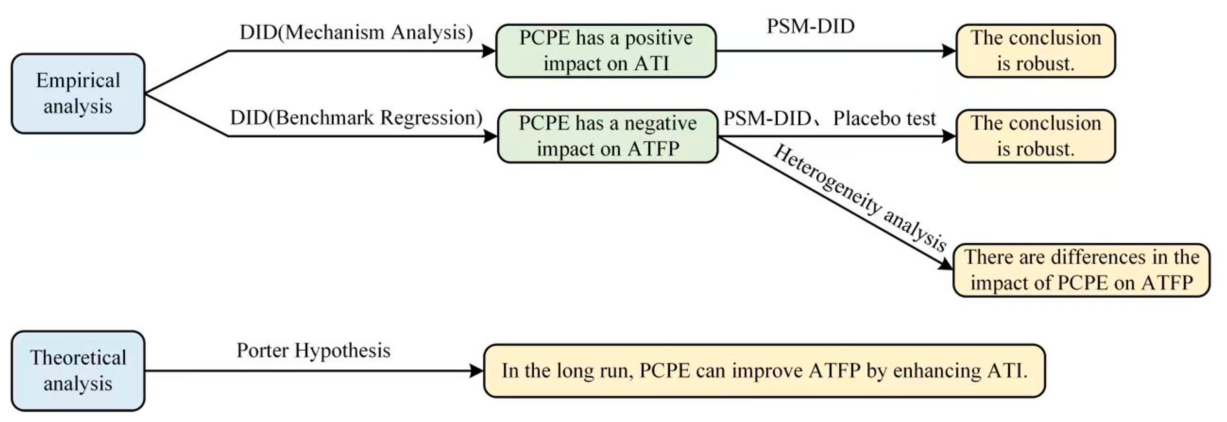
The results indicate that, although PCNPE initially exerts a negative effect on ATFP, it promotes agricultural technological innovation over time. In line with the Porter hypothesis, the innovation driven by the policy can eventually reverse its initial inhibitory effects, resulting in a long-term enhancement of agricultural productivity.
The potential marginal contributions of this study are as follows: (1) Focusing on prefecture-level cities in China, this is the systematically evaluation of the specific implementation effect of PCNPE based on multidisciplinary knowledge in different regions and its mechanism of impact on ATFP. This bridges the gap in empirical research on agriculture that mostly only examines the knowledge of a single discipline. (2) It investigates how restrictions on key agricultural production inputs such as nitrogen and phosphorus affect agricultural production, revealing that, while phosphorus restriction has a significant impact on ATFP, nitrogen restriction does not—although both factors are theoretically important for crop growth.
The remainder of this paper is organized as follows: Section 2 provides a literature review; Section 3 describes the theoretical framework and hypotheses; Section 4 outlines research design; Section 5 provides empirical results; Section 6 addresses heterogeneity analyses; Section 7 explores the underlying mechanisms; Section 8 is a comprehensive discussion and suggestions for policy optimization; Section 9 presents the limitations and prospects of the research.

2. Literature Review

2.1. The Impact of Environmental Regulation on ATFP

In recent years, the Chinese government has strengthened environmental regulation (ER) to enhance total factor productivity (TFP) and promote high-quality economic development [10]. The Porter hypothesis suggests that appropriate ER can stimulate corporate innovation, offsetting the production costs induced by regulation and ultimately enhancing productivity [13]. Empirical studies confirm that the annual average growth rate of TFP in China’s agricultural sector is about 1.5%, with technological progress being the primary driver. This supports the view that ER can promote technological advancement, improve production efficiency, and enhance the quality of agricultural products, thereby boosting the sector’s overall productivity and validating the Porter hypothesis in China’s agricultural context [14,15]. Moreover, ER can foster green technological innovation among agricultural producers. Under the combined pressures of external regulation and internal motivation, ER enhances local production efficiency and generates spillover effects that benefit surrounding areas [16]. For example, research on India’s sugar industry has shown that compliance with environmental regulations and water conservation initiatives has improved firms’ technical efficiency, in line with the Porter hypothesis [17]. This demonstrates that ER has played a positive role not only in China but also in other countries’ agricultural sectors, underlining its broad applicability in promoting production efficiency.
Although ER increases compliance costs for regulated entities, it simultaneously drives innovation and enhances product value [18]. Research shows that there is a threshold effect in the relationship between ER and agricultural TFP: Once this threshold is exceeded, optimizing the industrial structure can mitigate ER’s negative impacts on agricultural production [19]. In Europe, the implementation of environmental regulations has led to increased environmental R&D investment—a key input for knowledge production—resulting in more patent applications and highlighting the powerful role of ER in fostering innovation [20]. Technological advances spurred by ER help agricultural producers to offset compliance costs, improve management practices, and optimize resource allocation in response to regulations. These improvements jointly contribute to enhanced agricultural TFP [21,22,23].
Furthermore, ER reduces the waste of fertilizers, labor, and machinery inputs and encourages the adoption of more efficient production and management methods in the agricultural sector, thereby improving output efficiency [24]. Recent research [25] shows that agricultural mechanization significantly promotes green TFP by enhancing management levels, optimizing factor allocation, and diversifying the industrial structure. Rational input allocation eliminates resource misallocation, thereby improving both resource utilization efficiency and overall production capacity [6]. Therefore, environmental regulation can reduce the cost of ATFP growth, improve production efficiency and output, and promote the sustainable development of agriculture by optimizing the allocation of agricultural inputs [26].
An increase in TFP implies a higher output-to-input ratio. Further studies reveal that ER not only improves environmental conditions but also enhances growth resilience [27,28]. Therefore, ER helps reduce resource consumption and pollution emissions in agricultural production, achieving a win–win outcome for economic growth and environmental sustainability by fostering technological progress and industrial structure optimization [29]. From the perspective of urban–rural differences, research finds that rural areas are more dependent on land inputs, and low-income indicators in agricultural production areas are more resistant to policy shocks. In contrast, urban areas are more capital- and technology-intensive. Land use efficiency in eastern regions, in particular, drives growth potential under regulatory constraints [30]. These findings suggest that, when examining the impact of ER on agricultural TFP, it is crucial to account for regional variations in economic structure and resource endowments.

2.2. The Impacts of Nitrogen and Phosphorus on Crops and the Environment

Yield and growth of crops rely on a number of factors among which nitrogen and phosphorus play a crucial role in plant growth. Proper application of nitrogen and phosphorus fertilizer is essential to increase yield and quality of crops. Long-term deficiency of nitrogen and phosphorus depletes soil fertility and hinders crop growth and nutrient absorption [31]. Adequate nitrogen and phosphorus fertilizer application helps maintain soil fertility and supports healthy crop development. However, excessive phosphorus fertilization, particularly when combined with nitrogen deficiency, can increase phosphorus runoff, leading to water eutrophication [32]. ER can, through policy guidance, optimize fertilizer usage, improve nutrient-use efficiency, reduce environmental impacts, and enhance the overall ecological health of agricultural systems [33,34].
Soil serves as a vital medium for plant nutrient uptake, directly influencing crop growth [35]. Research shows that nitrogen enrichment promotes soil microbial diversity and boosts microbial activity [36,37]. Soil microbial communities, which affect crop growth and yield, respond differently to nitrogen and phosphorus fertilizers depending on crop rotation and growth stages. Tailoring fertilization practices to specific soil conditions can significantly improve the absorption of nitrogen and phosphorus, enhance soil structure and nutrient content, raise crop productivity, reduce costs, and ultimately improve ATFP [38,39,40]. China’s agricultural development reflects unique national characteristics, including limited agricultural labor and land resources, regional economic disparities, and localized governance structures. For instance, eastern coastal regions focus on high-tech agriculture and industrialization, while western regions prioritize infrastructure development and farmers’ incomes. These differences have shaped China’s agricultural systems and policies, generating experience with high transferability and wide applicability. Against this backdrop, studies on Chinese agricultural policy reveal that coordinated crop conversion strategies can significantly reduce environmental impacts while boosting farmers’ incomes [41]. This integrated approach provides useful references for agricultural policy interventions and offers new insights into how ER influences agricultural TFP through adjustments in crop structure.

3. Theoretical Analysis and Hypotheses

Nitrogen and phosphorus are essential for crop growth. Most fertilizers contain significant amounts of these elements. After implementing pilot policies controlling nitrogen and phosphorus, fertilizer use is restricted, reducing soil-absorbable nitrogen and phosphorus and directly affecting crop yield and quality [42]. Nitrogen is involved in crop metabolic cycles, and phosphorus is closely related to root development and energy conversion. Reasonable nitrogen and phosphorus control aims to optimize their use efficiency, prevent resource waste and environmental pollution from overuse, and ensure long-term agricultural sustainability and output [43]. In the short term, such policies affect fertilizer input but also promote agricultural technological innovation. Many innovations, especially in efficient fertilizer use, now focus on improving nitrogen and phosphorus efficiency and reducing reliance on high nitrogen and phosphorus inputs to meet policy requirements and production needs [44]. For example, precision agriculture technology precisely controls fertilizer application rates and timing, optimizes nitrogen and phosphorus supply, improves fertilizer efficiency, cuts waste and environmental pollution, and ensures crop growth. This shows that nitrogen and phosphorus control policies drive agricultural technological innovation, enhancing the sustainability and environmental friendliness of agricultural production.
Essentially, restricting fertilizer use promotes the adoption of these agricultural innovations, further advancing agricultural technological progress and production efficiency. To offset potential yield losses, producers must enhance soil productivity through organic matter introduction, management technology optimization, and agricultural machinery system investment [25,45,46,47]. These measures require extra labor, financial, and technical support, increasing production costs to maintain yields comparable to those with high fertilizer inputs [48]. Under these circumstances, implementing nitrogen and phosphorus control measures can lower local agricultural TFP in the short term.
More importantly, nitrogen and phosphorus control policies may drive agricultural industrial structure adjustments. Producers may shift to crops with lower nitrogen and phosphorus dependency, which often have lower yields and total output [49]. While this reduces environmental burdens, it also lowers overall agricultural production efficiency. In regions dominated by food crop production, the adjusted crop structure may fail to achieve the same output level as the original production model in the short term [50]. Moreover, changing production methods entails greater total costs (e.g., adjusting crop growth environments and altering agricultural production factors), further hindering the improvement of agricultural TFP. A flowchart can be employed to illustrate the elements in the research mechanism and logically link them, thereby strengthening the rationale, as shown in Figure 2.
Based on the above discussion, the following hypothesis is proposed:
Hypothesis 1.
Short-term curtailment of ATFP increases will be achieved through imposition of policies to regulate nitrogen and phosphorus.
Environmental regulation exhibits a “U”-shaped effect on agricultural green transformation. As regulation intensity increases, agricultural green TFP is first suppressed and then promoted [51]. As part of environmental regulation, PCNPE may follow a similar dynamic path. Initially, PCNPE increases costs and requires production method adjustments, suppressing production efficiency. However, once PCNPE reaches a certain intensity, governments may adopt agricultural technology subsidies and other support to compensate for profit losses and encourage technological innovation [52]. As producers gradually adapt and utilize technological innovations, they enhance crop yield and quality [53]. In the long run, nitrogen and phosphorus control drive agricultural technological innovation, promote green transformation, and force the reconfiguration of production factors, thereby optimizing the production factor structure needed for sustainable agricultural development [26,54].
Overall, PCNPE will prompt agricultural producers to shift to cleaner and more advanced modes of cultivation while optimizing agricultural input structure, ultimately increasing efficiency in utilizing resources and ATFP [55]. In summary, this paper puts forward the following hypothesis:
Hypothesis 2.
Implementation of PCNPE will stimulate agricultural technology innovation (ATI) that will ultimately offset the initial negative impact on ATFP and eventually lead to long-run gains.

4. Research Design and Data

4.1. Econometric Model Design

This study treats PCNPE as a quasi-natural experiment and uses the DID approach combined with regression analysis to evaluate its impact on the ATFP of Chinese prefecture-level cities. The goal is to explore how agricultural production adapts under nitrogen and phosphorus emission constraints, thus testing Hypothesis 1. PCNPE was implemented in some prefecture-level cities starting in 2016. When selecting research samples, and based on the parallel trend assumption, the actual implementation strength and policy participation of local governments were considered. Ultimately, 164 prefecture-level cities from 2016 were chosen as research samples. In these samples, cities implementing the phosphorus emission control policy (PCPE) and the nitrogen emission control policy (PCNE) were set as the experimental group, while other prefecture-level cities with complete variables served as the control group. We find the net effect of PCNPE on ATFP with an econometric model.
This study follows up on existing literature on the DID framework [56] and leverages recent advances in econometric modeling to construct a DID regression model with two-way fixed effects. The exact econometric specifications are in Equations (1) and (2):
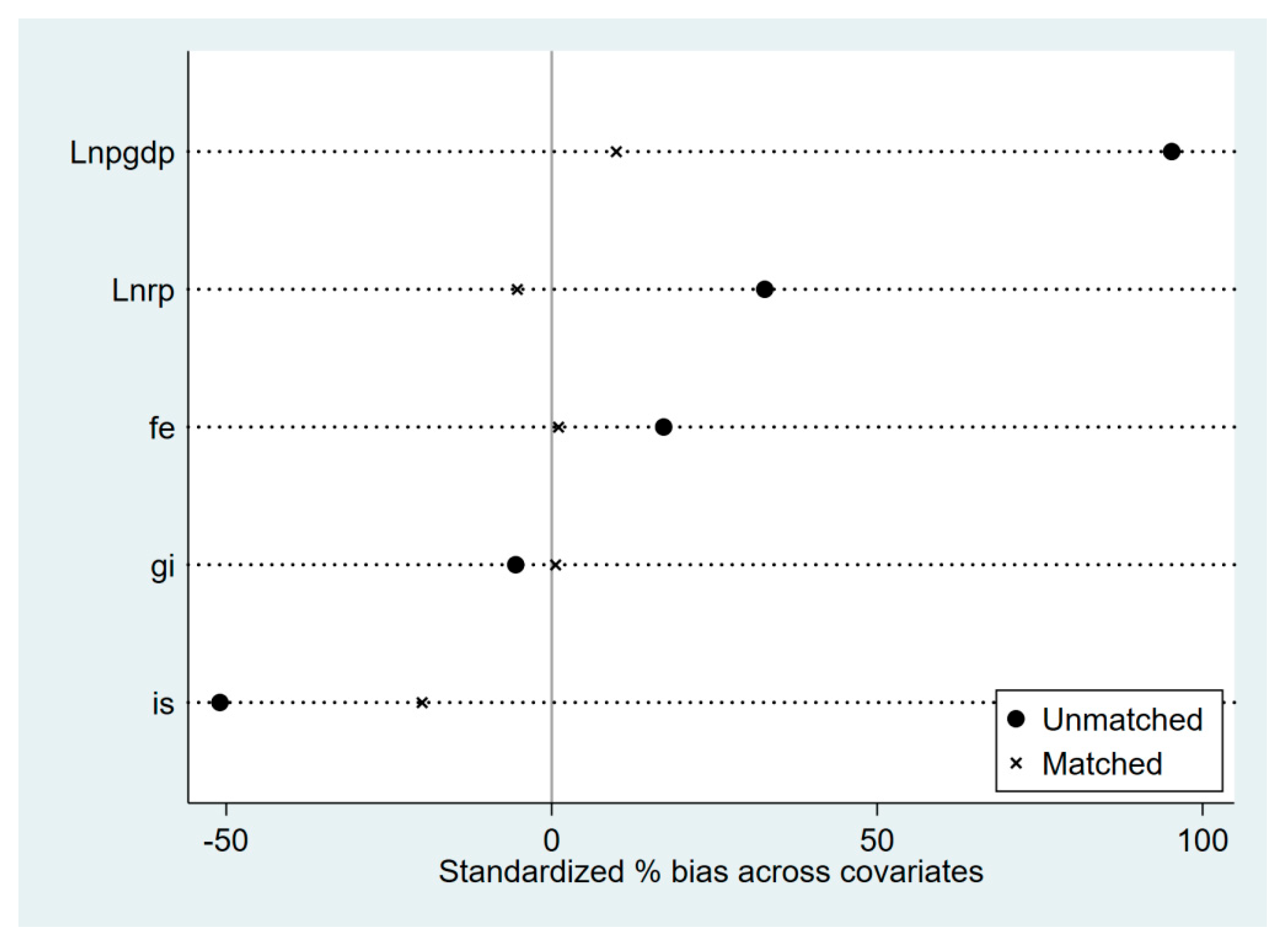
y i t = α 0 + α 1 n c × p o s t + β X i t + γ i + λ t + ε i t
y i t = α 0 + α 1 p c × p o s t + β X i t + γ i + λ t + ε i t
In the econometric model, y i t represents the ATFP level of prefecture-level city i in year t. α 0 is the intercept term of the model. α 1 denotes the regression coefficient of the interaction term between the dummy variable for total nitrogen and total phosphorus control areas and the policy implementation dummy variable, which is used to estimate the causal effect of PCNPE on ATFP. Nc and pc are dummy variables for total nitrogen and total phosphorus control areas, respectively. If a prefecture-level city belongs to a total nitrogen or total phosphorus control area in a given year, the variable takes a value of 1; otherwise, it is 0. Post is a dummy variable measuring the policy implementation period, which takes a value of 1 for the years when the policy was implemented (2016 and beyond) and 0 otherwise. The vector β represents the regression coefficients of control variables, capturing their impact on the dependent variable. The column vector X i t includes control variables such as: Economic development level (Lnpgdp), financial efficiency (fe), government intervention level (gi), industrial structure (is), and rural labor force level (Lnrp). The term γ i represents prefecture-level city fixed effects, which control for time-invariant characteristics of each city. λ t denotes year fixed effects, which account for differences among prefecture-level cities caused by time factors. ε i t is the random error term.
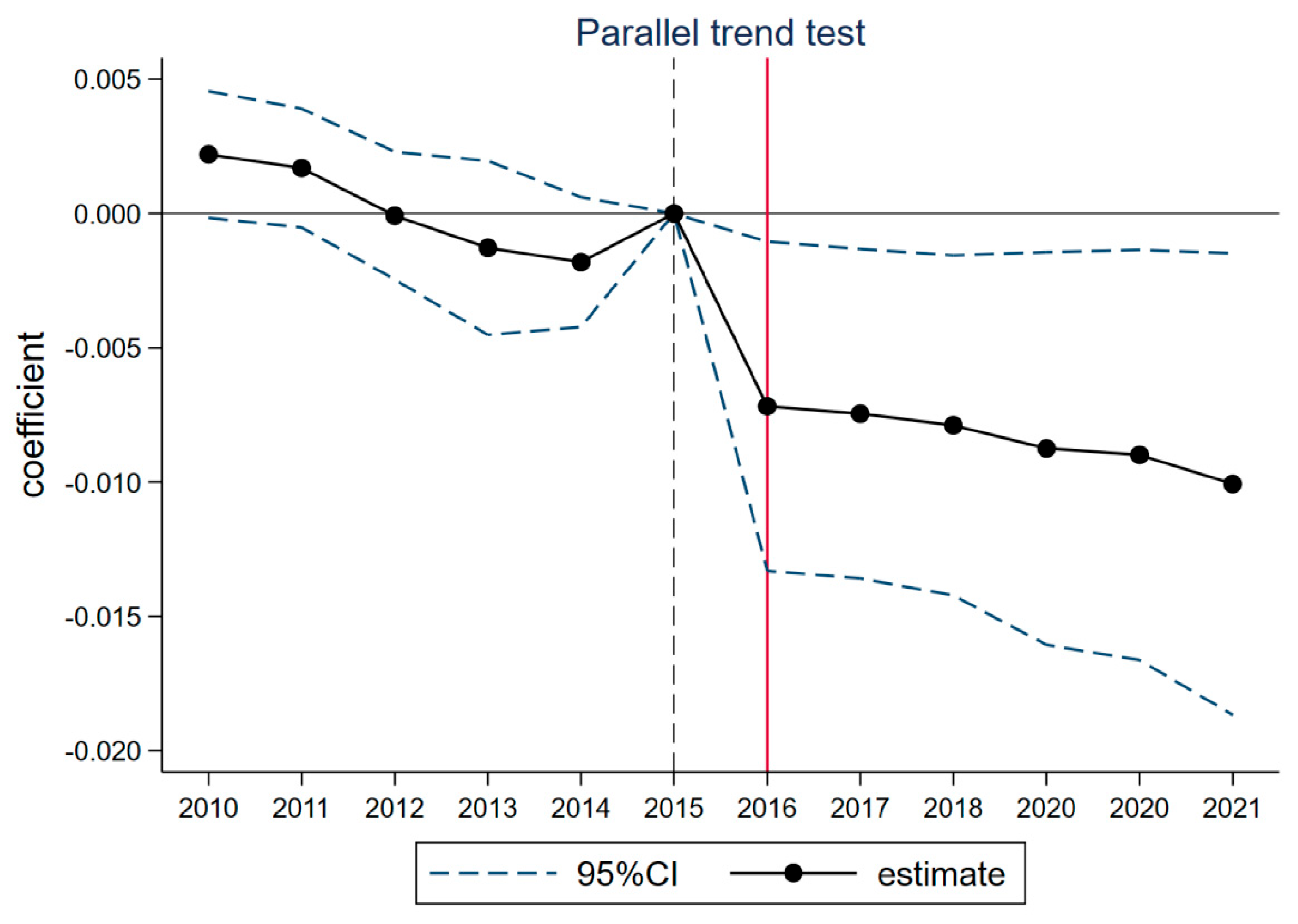
To ensure the unbiasedness of the DID estimates, it is crucial to verify whether the treatment and control groups satisfy the parallel trends assumption before PCNPE implementation. If this assumption is violated, the econometric model may yield biased estimates of the policy effects. Specifically, this study employs an event study method to conduct the parallel trends test, with the corresponding test equation given in Equation (3). Additionally, 2015 (the year prior to policy implementation) is selected as the baseline period to avoid strict multicollinearity issues.
y i t = α 0 + k = 4 T β k t r e a t i × D k t + δ X i t + γ i + λ t + ε i t
In the model, β k represents the coefficient of the interaction term between the k-period time dummy variable and the policy dummy variable, which is used to estimate the treatment effect for each period. t r e a t i is a treatment group dummy variable, indicating whether a prefecture-level city belongs to the experimental group for policy implementation. D k t represents the k-period time dummy variable, (e.g., D 2 t takes a value of 1 only in the year 2014, and 0 in all other years). The vector δ contains the regression coefficients of the control variables, while the meanings of the remaining symbols remain consistent with Equation (1).
Additionally, heterogeneity analysis is crucial for local policymaking, as different regions respond differently to policies. To explore the implementation of PCNPE across different regions and provide targeted improvements for existing policies, econometric models (Equations (4) and (5)) are established for further analysis.
y i t = α 0 + α 1 n c × p o s t + α 2 H i t + α 3 n c × p o s t × H i t + β X i t + γ i + λ t + ε i t
y i t = α 0 + α 1 p c × p o s t + α 2 H i t + α 3 p c × p o s t × H i t + β X i t + γ i + λ t + ε i t
In the model, H i t represents the heterogeneity variable of prefecture-level city i in year t. The coefficient α 2 denotes the regression coefficient of the heterogeneity variable, while α 3 represents the regression coefficient of the interaction term between the core explanatory variable and the heterogeneity variable. The meanings of all other symbols remain consistent with Equations (1) and (2).
Finally, this study establishes Equations (6) and (7) to test Hypothesis 2.
m i t = α 0 + α 1 n c × p o s t + β X i t + γ i + λ t + ε i t
m i t = α 0 + α 1 p c × p o s t + β X i t + γ i + λ t + ε i t
The model, m i t denotes the ATI level of the i -th prefecture-level city in year t , serving as a mechanism variable. The meanings of all other symbols are consistent with those in Equations (1) and (2).

4.2. Variable Selection and Construction

  • Dependent Variable
For ATFP measurement, we refer to recent literature [57,58,59] and adopt the slack-based measure data envelopment analysis (SBM-DEA) model of Tone (2001) [60]. The model does not rely on pre-specification of the production function but utilizes mathematical programming to calculate ATFP. In contrast to conventional methods, it does not rely on assumptions of functional form of the production function and therefore avoids functional form specification bias. The model also includes slack variables that allow full input and output slacks evaluation to avoid evaluation biases in conventional DEA methods that are constrained by radial and proportional changes. More importantly, comparative efficiency evaluation of decision-making units (DMUs) that operate on the frontier is facilitated by the SBM-DEA model. The mathematical specification of this model is shown in Appendix A.
In this context, θ * represents the measured ATFP of prefecture-level cities, M denotes the number of input indicators, and q represents the number of expected output indicators. s i and s i + denote the slack variables for the i-th input indicator, while s r and s r + denote the slack variables for the r-th expected output indicator. x i o t represents the observed value of the i-th input indicator at time t. y r o t represents the observed value of the r-th expected output indicator at time t. λ j t is the weight vector of the j-th decision-making unit at time t, and λ j t = 1 indicates constant returns to scale. Furthermore, x i j t and y r j t represent the values of the i -th input and r-th expected output indicators for the j -th DMU at time t , respectively. The relevant input and output indicators are presented in Table 1.
2.
Selection and Use of Core Explanatory Variables
The core explanatory variable is the interaction term between the policy dummy variable and the implementation time dummy variable. It is assigned a value of 1 if a prefecture-level city falls within a total nitrogen or phosphorus control zone in a given year; otherwise, it is 0. This interaction term measures the PCNPE policy implementation effect and is key to analyzing the policy’s impact on ATFP.
For PCNE, the experimental group comprises 22 prefecture-level cities with policy implementation and complete data, while the control group consists of 142 cities without policy implementation and complete data.
For PCPE, the experimental group includes 11 cities with policy implementation and complete data, while the control group comprises 153 cities without policy implementation and complete data. Figure 3 visualizes the two pilots.
3.
Selection and Use of Mechanism Variables
Based on Hypotheses 1 and 2, and drawing on relevant literature, this study selects the number of agricultural invention patents as a proxy for ATI [61,62]. Data are sourced from China’s National Intellectual Property Administration. This choice has several advantages: First, agricultural invention patents cover a wide range of fields, including agricultural machinery, chemical fertilizer production, agricultural product processing, and agricultural information technology, comprehensively reflecting the scope and depth of agricultural innovation. In contrast, the agricultural mechanization rate only reflects the popularity of machinery use, not the breadth of technological development. Additionally, patents have clear legal status and public availability, making them highly accessible and comparable for collection and analysis. Unlike R&D investment data, which is difficult to obtain and standardize due to varying accounting practices, patents directly indicate technological innovation outcomes.
4.
Control Variables: Choice and Application
We address the problem of endogeneity in this research by including the following control variables: Level of economic development, level of government intervention, rural labor force population, financial efficiency, and industrial structure. According to Faluk Shair et al. (2021) [63], economic development has a significant impact on production efficiency. Technological progress and optimal resource allocation enhance production efficiency and hence stimulate economic development. Therefore, to control for the likely impact of economic development on ATFP, this study employs the natural logarithm of per capita GDP as a control variable. This alleviates concern with regard to endogeneity such that regression coefficients more accurately reflect actual impacts. Additionally, Na Zhang et al. (2024) [64] found that government intervention positively affects production efficiency. Government intervention through administrative and fiscal policies can maximize resource utilization and reduce agricultural operating costs. Additionally, government intervention helps to steer agriculture to environmentally friendly and sustainable production techniques that enhance production efficiency while conserving the environment. Therefore, the fiscal expenditure and GDP data of the general budget of each prefecture-level city in the current year are used to calculate the ratio of the two to control the possible impact of government intervention on ATFP. Lastly, Yongchun Sun (2022) [65] emphasized that rural labor force size matters in ATI and ATFP. The organization and size of the rural labor force have a direct impact on agricultural production efficiency and output as well as on ATFP through technological substitution and human capital effects. As urbanization increases, agricultural labor moves to cities through rural-to-urban flows, resulting in labor shortages that force technological and mechanization progress in agriculture that enhances ATFP. Therefore, through statistical data such as the “Chinese Population and Employment Statistical Yearbook”, the rural population data of each prefecture-level city in the current year are obtained, and the natural logarithm is taken after adding 1 to control the impact of rural labor force size on ATFP. Above all else, Hu et al. (2021) [66] noted that the financial system is important in allocating resources. An effective financial system can lower agricultural enterprises’ cost of finance and ease finance constraints and eventually impact ATFP. For capturing financial efficiency, based on statistical data such as the China Financial Statistical Yearbook, this study uses the loan-to-deposit ratio (LDR) in prefecture-level cities as an indicator of financial efficiency. The LDR is a direct indicator of financial institutions’ ability to convert savings to investment and hence is a primary indicator of financial system efficiency. The higher LDR implies a more efficient transfer of capital to demand sectors from surplus sectors. Financial efficiency is hence utilized as a control variable in the regression equation. Lastly, Chen et al. (2023) [67] attested that industrial structure optimization not only increases technological progress and efficiency in allocating resources but also increases agricultural modernization through technology spillover effect and therefore increases ATFP. So, we introduce industrial structure as a control variable. Through statistical data such as the China City Statistical Yearbook, the added value of the primary industry and GDP data of each prefecture-level city in the current year are obtained, and the proportion of the added value of the primary industry in GDP is calculated to measure the industrial structure.
Lastly, by introducing such control variables, we effectively control over direct and indirect effects of economic development, government intervention, rural labor force size, financial efficiency, and industrial structure on ATFP. This alleviates concerns over endogeneity and ensures that the estimated coefficient of the core explanatory variable more precisely captures actual policy impacts. As such, reliability and accuracy of research findings improve and hence a more scientific basis exists to study factors influencing ATFP.

4.3. Sample Selection and Sources of Data

This study used panel data from 164 prefecture-level cities in China between 2003 and 2022, with cities with complete data as the control group to ensure the accuracy and reliability of the analysis and cities implementing PCNPE policies as the experimental group. The data include the following key economic and agricultural indicators: Per capita GDP, general government spending on government purchases, GDP, value added of the primary sector, and number of agricultural invention patents. These data are obtained from the China Regional Economic Statistical Database and the EPS Data Platform. The nitrogen and phosphorus control pilot program data are sourced from official Chinese government documents issued by the State Council, and dummy variables are manually constructed based on these policy documents. The LDR is derived from the China Prefecture-Level City Statistical Database available on the China Macroeconomic Data Platform. The rural permanent population data are collected from the Agricultural Statistical Yearbooks of various provinces and cities. To ensure data quality, we exclude prefecture-level cities with missing values for key variables. Moreover, to mitigate the impact of heteroskedasticity, we apply logarithmic transformations to non-ratio variables. The descriptive statistics and variable definitions after data processing are presented in Table 2.

5. Result Analysis

5.1. Benchmark Regression Results Analysis

In this study, to mitigate the impact of multicollinearity on estimation results, we employed stepwise regression to analyze the effect of PCNPE on ATFP. Specifically, we initiated the regression with only the core explanatory variables and gradually incorporated control variables. If the significance of the core explanatory variables remained unchanged after adding control variables, it indicated that their significance was not substantially affected by multicollinearity. The core explanatory variables were the interaction terms of policy dummy variables (nc or pc) and implementation time dummy variables (post), referred to as ncp and pcp, respectively.
The benchmark regression results presented in Table 3 show that, in models (1) to (6), the statistical tests of ncp failed to reject the null hypothesis that the regression coefficient of ncp was zero. This suggests that PCNE had no statistically significant impact on ATFP, meaning it failed to achieve the desired effects. In contrast, the benchmark regression results for PCPE in Table 4 indicate that, in models (1) to (6), the regression coefficients of pcp were significantly negative at the 5% level. Specifically, the estimated coefficients ranged from −0.013 to −0.015, indicating that PCPE had a statistically significant negative effect on ATFP in the short term. After including all control variables, the implementation of PCPE was found to reduce ATFP by approximately 0.013 units on average. Additionally, the statistical tests of the control variables did not reject the null hypothesis that their coefficients were zero, but their signs aligned with theoretical expectations. All models controlled for city and year fixed effects to account for time-invariant city characteristics and time-specific factors, which helped mitigate endogeneity issues and enabled a more accurate estimation of causal effects.
Phosphorus is essential for plant growth and development, and global food production heavily depends on phosphorus fertilizers. However, phosphorus resources are limited and unevenly distributed, and the management of phosphorus use is complex. Many crops grow in soils with low available phosphorus, where phosphorus fixation reduces its availability, thereby affecting crop yield and quality [68,69].
In summary, when both nitrogen and phosphorus uses are restricted, only phosphorus control significantly affects ATFP, suggesting that agriculture is more dependent on phosphorus under normal circumstances. The significant negative effect of PCPE on ATFP in the short term, but not PCNE, highlights the key role of phosphorus and its critical importance to crops [70].
The R2 values of the models ranged from 0.262 to 0.264, indicating minimal change in model explanatory power with the addition of control variables. However, after applying propensity score matching (PSM), the R2 value increased to 0.401. This demonstrates that PSM enhanced the model’s explanatory power and confirmed the validity of the control variable selection. By reducing selection bias, PSM made the treatment and control groups more comparable, thereby enhancing the significance of the control variables. This implies that, prior to matching, the effects of the control variables might have been underestimated due to sample selection bias. Consequently, subsequent model validation and sensitivity analyses should adequately consider the matching effects to ensure the robustness and reliability of the results.

5.2. Parallel Trend Test

Another crucial requirement for the validity of the DID strategy is that the control group and treatment group share a common parallel pre-policy trend [71]. In the case of benchmark regression estimation, it was discovered that PCPE had a significant adverse effect on ATFP. Therefore, in the remainder of this discussion, we take into account PCPE alone. Prior to PCPE implementation, it is important to verify that the treatment and control group prefecture-level cities had a parallel trend in ATFP. In particular, this study uses the event study framework to determine if the treatment group and control group had a parallel trend prior to intervention. The year 2015 (pre-policy implementation year) is used as the baseline year [72,73,74] and is presented in Figure 4. The parallel trend test results show that, prior to intervention (pre-2015), all periods of event estimates fall within the 95% confidence level. This suggests that, at a 5% significance level, we cannot reject the null hypothesis that treatment and control group cities had a pre-intervention parallel trend. Moreover, after intervention (2016 and later), event estimates of 2016 to 2021 are statistically significant at a 5% level. This suggests that the benchmark regression findings are reliable and that PCPE had a prompt effect in the intervention year (2016), with policy impacts lasting long after.

5.3. PSM-DID

When applying the DID strategy to evaluate the impact of PCPE on ATFP, differences in characteristics between treatment and control groups can lead to biased treatment effect estimations. In order to eliminate selection bias effects, we follow Heyman et al. (2007) [75] and use the nearest-neighbor many-to-one matching without replacement to match treatment and control groups before applying DID analysis (i.e., PSM-DID). This strategy attempts to reduce estimation bias by estimating control group propensity scores and selecting control group members that are similar to the treatment group on multiple dimensions before statistical estimation. Figure 5 and Figure 6 display kernel density function curves pre- and post-matching, respectively. Before matching, the treatment group has a higher central point and mean propensity score than that of the control group. Post-matching, both of these measures for the treatment group nearly match those of the control group. This suggests that applying differences between the two groups without matching would lead to extreme estimation errors. Furthermore, Figure 7 provides balance test results that show that differences in covariates between groups are considerably reduced after matching, indicating that the matching procedure is effective in eliminating likely differences between treatment and control groups and enhances the credibility of comparative study. Finally, in Table 5, columns (1) and (2) report regression results using samples with non-zero matching weights and those with a common support assumption, respectively. The results indicate that the regression coefficient of the core explanatory variable (pc) is negatively significant at 1% in column (1) and negatively significant at 10% in column (2). In addition to this, the absolute value of the estimated coefficient after PSM-DID is much higher than that after using the benchmark regression. This indicates that, if matching were not performed and straightway DID were to be used, it would result in underestimation of the negative effect of PCPE on ATFP. Overall, the estimated coefficients after PSM-DID have the same sign as those after using the benchmark regression, thereby confirming the robustness of benchmark regression results.

5.4. Placebo Test Analysis

1.
Time Placebo Test
To offer more confirmation of the robustness of the benchmark regression results, we conduct a time placebo test. Following Mengqi Ding (2023) [76], this study carries out a placebo test on the time of policy implementation to make sure that previous findings were not caused by random time-related factors. Specifically, we artificially shift the time of policy implementation several years back to generate a fictional time of policy implementation and then examine if in such fictional time periods the estimated treatment effect strongly rejects the null hypothesis of zero effect. For each false time point: A new post variable was defined (e.g., 2015 instead of 2016 as the policy start year). Fake interaction terms (fake ncp and fake pcp) were created by multiplying the policy dummy variables with the new post variable. ATFP was regressed on the fake interaction terms and other controls to check if the coefficients were significant.
The results are presented in Figure 8. The x-axis shows the hypothetical policy implementation times (years before the actual policy year). The y-axis shows the estimated placebo effects. The estimated placebo effects fluctuate slightly over time, but all their 95% confidence intervals include zero. Thus, the placebo effects are statistically insignificant, supporting the conclusion that the original policy effects are not due to time-related random factors. Specifically: When setting the false policy year 1 year earlier, the placebo effect estimate is close to zero. When setting the false policy year 2 or 3 years earlier, the estimates decrease slightly but still fall within the confidence interval. When setting the false policy year 4 years earlier, the estimates increase but remain insignificant. This consistent pattern demonstrates that only the actual policy implementation time generates significant effects, further confirming the robustness and credibility of the benchmark regression results.
Moreover, throughout the placebo test: City and year fixed effects were retained to control for potential time-invariant city-specific and annual characteristics. Logical and realistic false policy years were chosen to avoid unreasonable bias. These detailed settings and robustness checks strongly support the reliability of the conclusions that PCPE significantly negatively impacts ATFP.
2.
Random Spatial Placebo Test
To more definitively exclude that the benchmark regression result was due to random factors in prefecture-level cities, this study extends the time placebo test with a spatial placebo test. Specifically, besides randomly selecting a pre-2016 year as a hypothetical year of fictitious implementation of policies, we also randomly select a group of prefecture-level cities—the same number as that of the treatment group in benchmark regression—as a new experimental group before estimating the treatment effect. We adopted the procedure of Lifeng Chen (2022) [77], randomly selecting k prefecture-level cities without replacement with k being same as the number of cities in the original treatment group, and then repeat benchmark regression 500 times. The result of the spatial placebo test after 500 rounds is reported in Figure 9. In Figure 9, the blue line is kernel density estimation of placebo effects with roughly symmetric distribution centered around zero resembling a normal distribution. The red dashed line is the zero effect value with no treatment effect as the baseline. The benchmark regression estimate (red vertical line) is at the right tail of the distribution far away from the center. This indicates that the observed policy effect is far away from center of the distribution of randomly sampled treatment effects. Thus, the result of the spatial placebo test again confirms the robustness of the benchmark regression outcome and that it is unlikely due to random factors at either the temporal or prefecture-city level.

6. Heterogeneity Analysis

6.1. Heterogeneity in Environmental Protection Zones

This study continues to examine the impact of PCPE in key areas of environmental protection. In line with China’s “11th Five-Year Plan for National Environmental Protection” promulgated by the State Council in 2007, 112 cities were designated as key environmental protection cities. The ifep variable is utilized to identify if a city is situated in a key environmental protection zone (1 = Yes, 0 = No). The benchmark regression results show that PCPE negatively impacts ATFP in all regions. However, the impacts of PCPE implementation vary by region. The environmental protection zone-based heterogeneity is presented in column (1) of Table 4. The results show that the pcp × ifep interaction term is positive at the 1% level (coefficient = 0.021, t-statistic = 3.49). This suggests that, compared with non-key environmental protection areas, the adverse effect of PCPE on ATFP is smaller in key environmental protection areas. This finding suggests that agricultural producers in key environmental protection areas have already adjusted to PCPE. The presence of pre-existing stringent environmental regulations has likely counterbalanced the adverse effect of PCPE to preserve ATFP levels. More specifically, agricultural producers in such areas may have already adopted green technologies [78,79] that meet environmental standards and thus become more flexible to adapt to PCPE requirements and thus reduce the initial shock to agricultural production. Furthermore, key environmental protection areas have more experience in environmental management and enough reserves of resources to reduce their marginal adverse effect of new environmental regulations on ATFP.

6.2. Geographical Heterogeneity

Geographic diversity is also due to climatic variations that lead to regional diversity in crops that are planted (e.g., wheat in northern China and rice in southern China). The effects of nitrogen and phosphorus on crops also differ. Regional diversity in implementation of policies and agricultural production technology is also present. Therefore, it is essential to study the diverse impacts of PCPE at different geographical locations to provide information to regional governments. This study investigates the regional heterogeneity of PCPE impacts on ATFP across two spatial dimensions: The east–central–west economic zoning and the Qinling–Huaihe natural divide between northern and southern China.
The east–central–west analysis uses the 2003 Economic Zoning Standard by China’s National Bureau of Statistics, categorizing regions into eastern, central, and western zones. In this framework, the western region is treated as the reference group. Dummy variables are constructed to indicate central (ifemw (mid) = 1) and eastern (ifemw (east) = 1) regions, with 0 indicating western regions. Results from the heterogeneity test, presented in column (2) of Table 6, show that the interaction term pcp × ifemw (mid) is positive and significant at the 5% level (0.017), indicating that the negative impact of PCPE on ATFP is weaker in central regions compared to the west. Similarly, the interaction term pcp × ifemw (east) is positive and significant at the 1% level (0.023), suggesting that the eastern region experiences an even smaller negative effect than the west. These outcomes suggest that, in the short term, the reduction in ATFP caused by nitrogen and phosphorus restrictions is less pronounced in central and eastern China. This can be attributed to higher levels of agricultural technology, more environmentally friendly production systems, and reduced dependence on excessive nutrient application in these regions [80].
The second dimension of heterogeneity considers the natural geographic division between northern and southern China, based on the Qinling–Huaihe boundary. A dummy variable ifn = 1 is used to indicate whether a region is located in the north. Column (3) of Table 6 presents the results for this dimension. The coefficient of the interaction term pcp × ifn is statistically insignificant, indicating no significant difference in the effect of PCPE between northern and southern regions.
Although the two regions differ in climate, soil conditions, and crop structure, these differences do not appear to translate into variations in PCPE outcomes. In northern China, cold and dry climatic conditions lead to a saturation of soil phosphorus, reducing the marginal productivity of additional phosphorus fertilizer. The phosphorus yield-increasing effects thus decline, limiting the region’s dependence on phosphorus inputs [81,82]. Conversely, in southern China, warm and humid weather creates acidic soils that limit phosphorus availability. Phosphorus tends to bind with calcium ions, forming insoluble calcium phosphate, which contributes to phosphorus loss and deficiency [83,84,85].
Despite these agronomic contrasts, the overall effect of PCPE remains similar across the north and south. This may be due to shifts in farmers’ fertilizer application strategies. In the north, crops such as wheat and corn demand more nitrogen than phosphorus, making nitrogen a more critical yield determinant [86,87]. Therefore, nitrogen adjustment strategies are prioritized over phosphorus use. Additionally, northern climatic conditions, particularly colder temperatures and shorter growing seasons, slow the mineralization process of phosphorus in soil, further decreasing the need for phosphorus fertilizers [88,89].
In southern China, although rice cultivation demands more phosphorus, acidic soils reduce its uptake efficiency. Farmers often rely on irrigation systems and organic manure as substitutes to maintain productivity under phosphorus constraints [90]. Therefore, even with varying agricultural practices and biophysical environments, the implementation effects of PCPE remain statistically similar between the two regions.

7. Mechanism Analysis

This section tests Hypothesis 2 that PCPE promotes ATFP in the long run by fostering ATI. The empirical results (shown in 
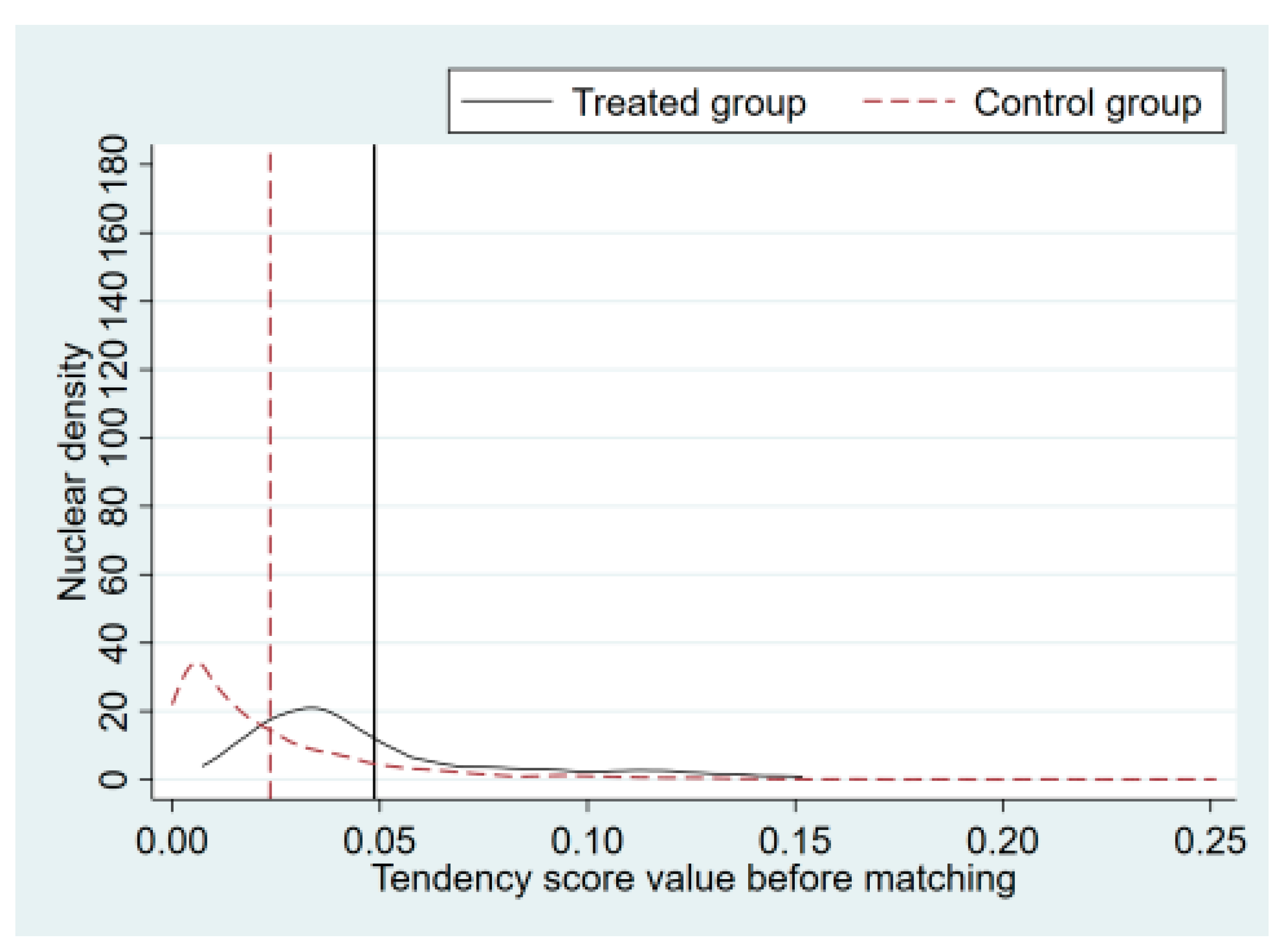
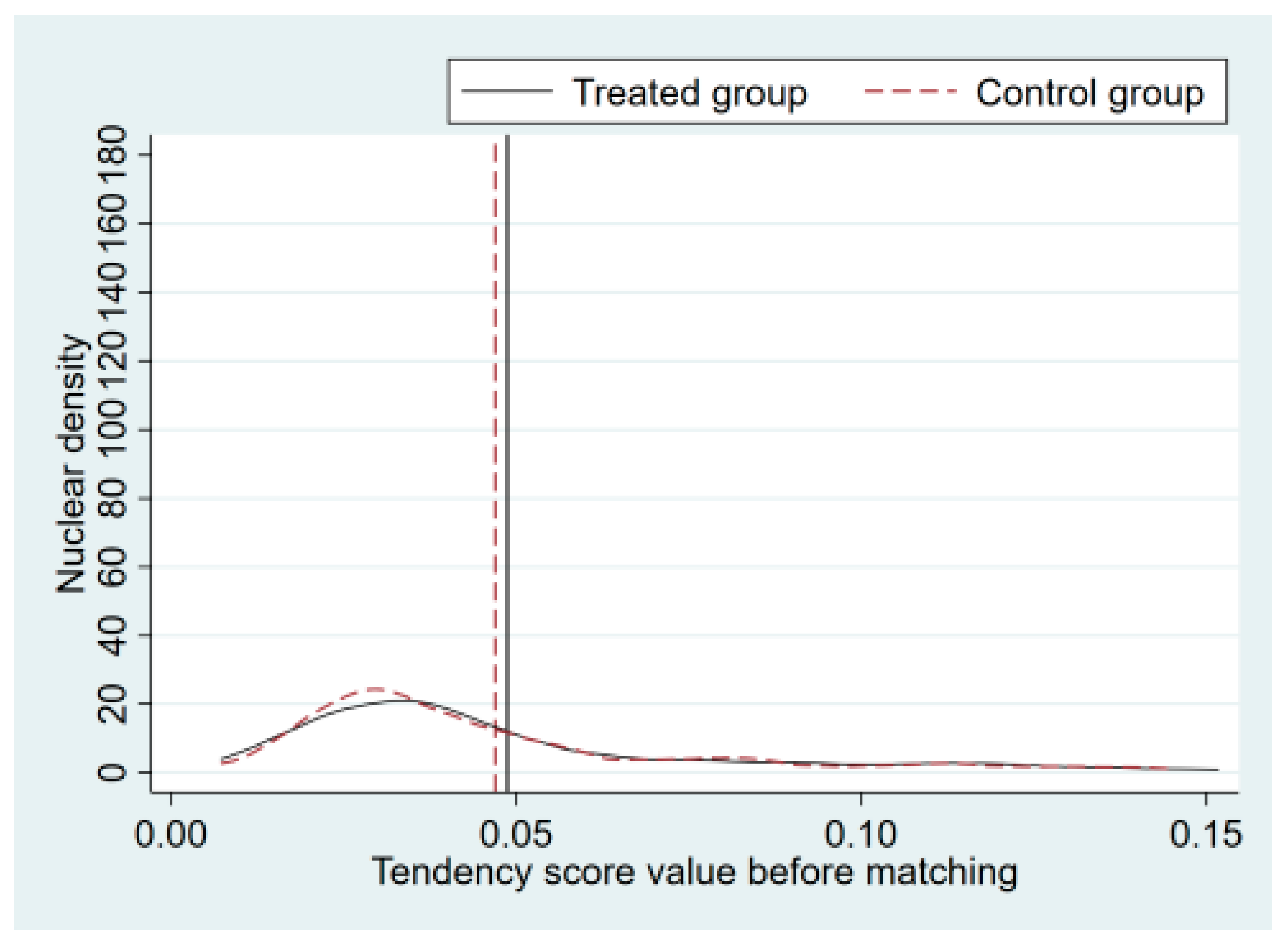
Table 7) reveal that, when replacing the dependent variable with Lntpa and using stepwise regression (columns (1)–(6)), the core explanatory variable pcp has a significantly positive coefficient at the 1% significance level. This indicates that PCPE indeed promotes ATI, which subsequently enhances ATFP, thus supporting the “Porter hypothesis”. On average, PCPE can increase ATI by approximately 2.1%. Column (7) presents the PSM-DID regression results. Here, pcp remains significantly positive at the 5% level (t-value = 2.24), with a coefficient of 0.071. This finding confirms that PCPE continues to have a positive effect on ATI even after addressing potential endogeneity through PSM-DID. Overall, these results provide strong evidence supporting the conclusion that PCPE promotes ATI, thereby boosting ATFP over time. This empirical validation strengthens the credibility of the theoretical analysis. Existing literature [91,92,93,94] also identifies ATI as a crucial mechanism linking PCPE to ATFP. By improving agricultural technologies and management practices, optimizing resource allocation, and increasing crop yields and quality, ATI ultimately enhances ATFP. Thus, the mechanism analysis empirically confirms Hypothesis 2.
The promotion of ATI by PCPE is reflected in several specific policy measures: Government-funded agricultural research projects: Direct investment into research programs accelerates the development of new technologies. Increased R&D investment: Dedicated resources for innovation foster breakthroughs in agricultural production. Tax incentives: These reduce innovation costs for agricultural firms, encouraging technological upgrading. Technical training subsidies: These enhance farmers’ skills and accelerate the diffusion of new technologies. These measures collectively create a favorable innovation environment, promoting effective interaction among governments, research institutions, enterprises, and farmers and forming a strong innovation synergy.
ATI covers various technological domains: Biotechnology: Enhances crop resistance to pests and diseases, reduces pesticide use, and improves crop quality. Information technology: Enables precision agriculture through GPS, sensors, and data analytics, optimizing field management and boosting production efficiency. Engineering technology: Drives the automation and intelligent operation of agricultural machinery, enhancing operational efficiency and promoting large-scale, standardized farming. These technological innovations complement each other in driving improvements in agricultural productivity.
The impact of PCPE on ATFP exhibits a phased nature:
Short term (1–2 years after implementation) [95,96]: Baseline regression shows that PCP has a negative effect on ATFP because the time horizon of the study sample is not long enough, ATI needs time to work, and it has not accumulated enough returns to reverse the negative effects. Specifically, the introduction of new technologies needs to overcome the problem of farmers’ learning cost and technology adaptability, which may lead to a temporary decline in production efficiency. The high initial investment of ATI, such as equipment purchase, technical training, and infrastructure construction, is difficult to compensate for through increased output in the short term, which has a negative impact on ATFP [57]. In addition, the imperfection of the technology promotion system may also lead to information asymmetry and technology misuse, which will exacerbate the short-term negative impact.
Medium term (3–5 years after implementation) [97,98]: Some of the ATI results invested in the early stage were gradually applied and promoted, and some farmers initially mastered the new technology, and the learning cost was reduced. The weak links of the technology promotion system have also been improved, the threshold for technology application has been lowered, and the negative impact of ATI on ATFP has gradually decreased, but the positive effect has not yet fully appeared.
Long term (over 5 years after implementation) [99,100]: The technology is mature, the promotion system is perfect, and the positive effect of ATI is gradually emerging and enhanced. The maturity of the technology is reflected in the improvement of performance, the reduction of costs, and the acceleration of technology diffusion. Agricultural R&D continues to advance, and new technologies continue to emerge and be adopted by more farmers, improving the overall efficiency of agricultural production and significantly positively impacting ATFP. The perfect extension system lowers the threshold for technology application, reduces the learning cost of farmers, accelerates the popularization of new technologies, and promotes continuous improvement and optimization of technologies. This long-term effect reflects ATI’s central role in sustainable agricultural development and its far-reaching impact on production efficiency [101].
In summary, ATI enhances ATFP by: Optimizing production efficiency, improving resource allocation, introducing new production and management methods, reducing resource inputs per unit of output, and enhancing the efficiency of labor, capital, land, and natural resources. Technological progress streamlines production processes and enables more effective resource utilization, ultimately driving sustained improvements in agricultural TFP [102,103].
Thus, although PCPE may have short-term negative effects, it promotes long-term productivity gains by fostering agricultural technological innovation.

8. Conclusions and Recommendations

8.1. Conclusions

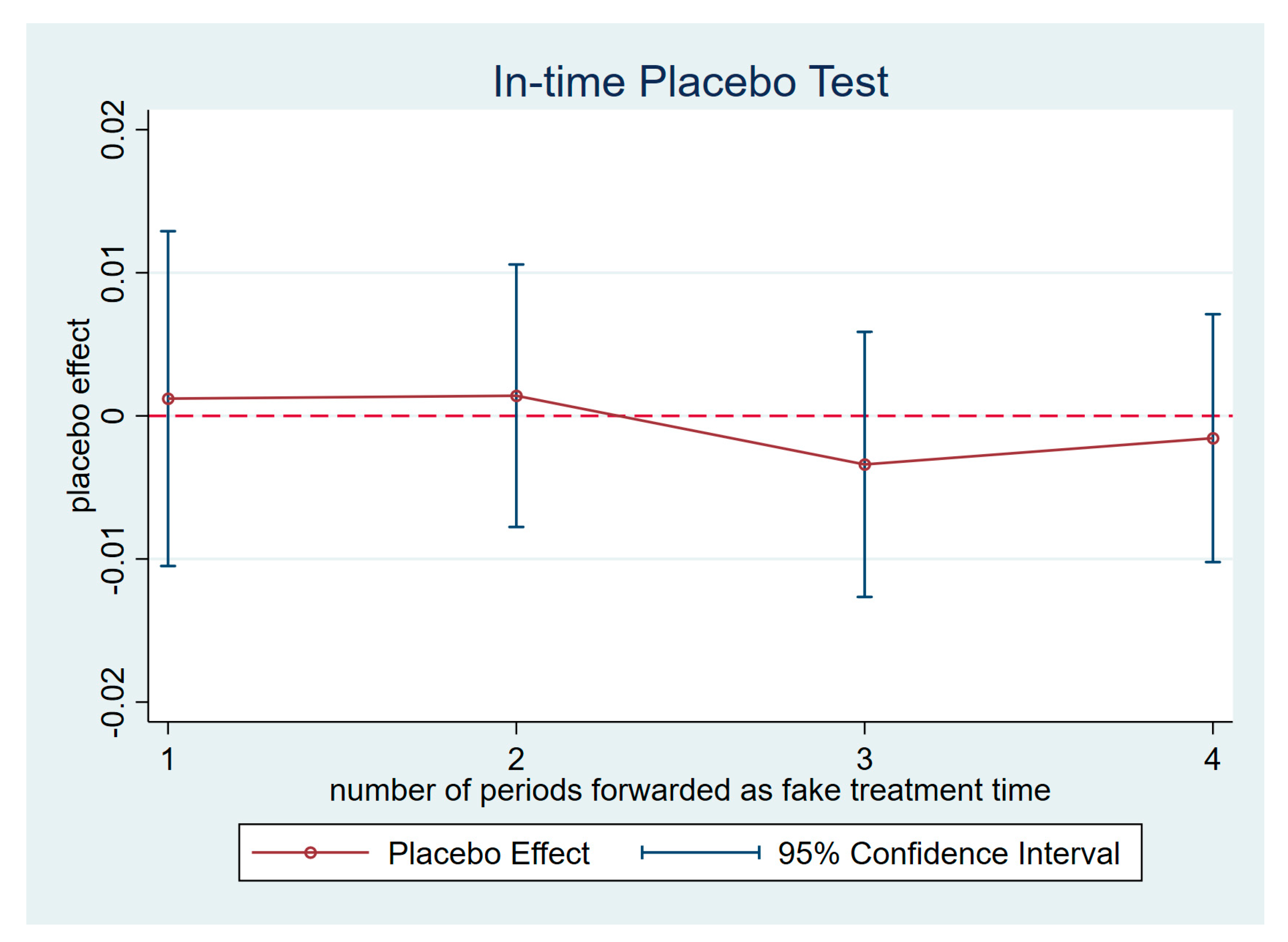
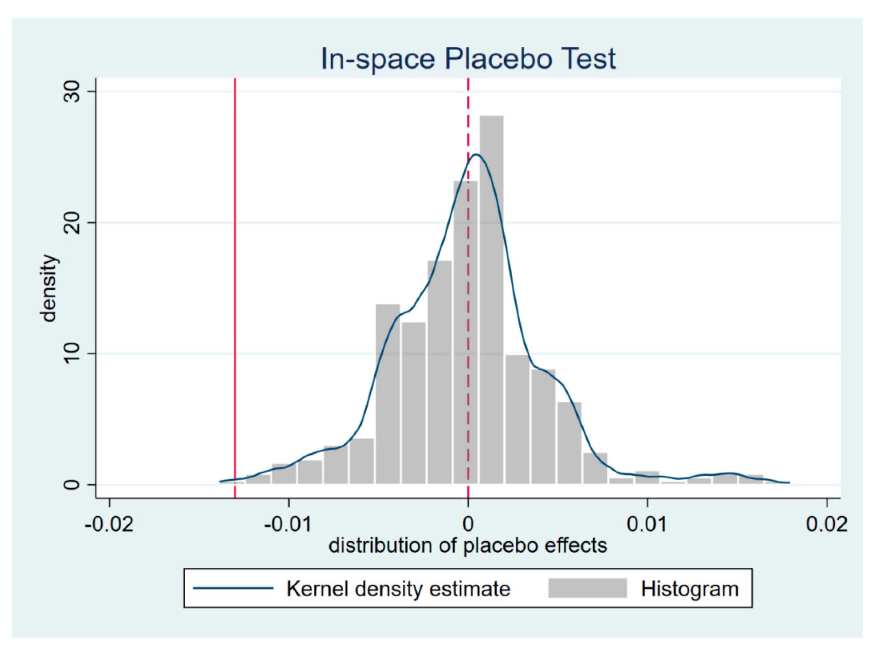
Since China is facing the challenge of reconciling agricultural production expansion with environmental sustainability, it is crucial to design environmental regulations that both maintain the ecosystem and enhance ATFP. In response to this challenge, this study constructs a quasi-natural experiment setting and employs panel data spanning 164 prefecture-level cities in China between 2003 and 2022. The impact of PCNPE implementation on ATFP and its mechanism is analyzed using DID augmented with regression analysis. The results indicate that, in the short run, after controlling other determinants of ATFP, PCPE reduces ATFP by approximately 0.013 units on average while PCNE does not have a statistically significant impact on ATFP. This suggests that agricultural production is dependent to a larger extent on phosphorus than nitrogen. In addition, restricting phosphorus application in the short run suppresses ATFP. After subjecting findings to robustness tests including parallel trend tests, PSM-DID, and placebo tests, the conclusions remain valid. The heterogeneity analysis shows that, in contrast to non-key environmental protection areas, the adverse effect of PCPE on ATFP is smaller in key environmental protection areas. This suggests that accumulating environmental technologies can minimize environmental regulation policies’ adverse effect on ATFP. In addition, PCPE’s effect is smaller in suppressing ATFP in the central and eastern regions relative to the western region, indicating that these regions are more resistant to environmental regulations. More notably, even with variations in climate and crops between northern and southern China, PCPE’s effect on ATFP does not differ substantially between the two regions. Finally, according to Porter’s hypothesis, this study establishes that PCPE enhances ATFP in the long run by developing ATI. Briefly, this research provides new empirical evidence of Porter’s hypothesis in agriculture and presents biological and chemical information that can be used to inform policymakers who desire to balance agricultural production with environmental conservation.

8.2. Policy Recommendations

First, although the implementation of PCPE results in a short-term decline in ATFP, it can promote ATI and enhance ATFP in the long run. Thus, policymakers should focus on refining PCPE measures and expanding pilot programs to achieve the dual goals of environmental protection and high-quality agricultural development. Drawing on international experience, such as the European Union’s Horizon Program, the Chinese government could: Increase support for green agricultural technology R&D, establish special funds for technologies that replace phosphate fertilizers and restore soil health, and set up ATI centers to accelerate the mastery and application of new technologies by producers.
Second, considering regional differences in response to PCPE, policies should be tailored to local conditions: In key ecological protection areas, “technology–policy synergy” pilots could leverage existing environmental technologies to better balance ecological and production goals. In non-key areas, innovation subsidies should prioritize environmental technologies to promote cleaner production. In the central and eastern regions, continued investment in ATI is needed to enhance resilience to regulatory shocks. In the western region, efforts should focus on improving phosphorus fertilizer efficiency through infrastructure enhancement and farmer training. Additionally, the government should encourage technical cooperation between eastern and western regions to promote agricultural modernization across the country. For areas facing short-term productivity losses, governments can refer to policies such as the “Conservation Reserve Program” in the United States (https://www.farmers.gov/sites/default/files/2022-05/farmersgov-conservation-programs-brochure-05-2-2022.pdf, accessed on 25 March 2025.). By providing financial compensation, technical assistance and financial support, we will help local agricultural producers tide over the difficulties and mitigate the negative impacts in the early stages of policy implementation.
Finally, to strengthen support for agricultural innovation, besides financial support, intellectual property protection should be enhanced to encourage participation from enterprises, research institutions, and individuals. A robust technology promotion system should be established through technical training, field demonstrations, and farmer field schools, accelerating the adoption of new technologies and maximizing their impact. These measures can effectively boost ATFP and achieve a win–win outcome of high-quality agricultural development and environmental sustainability.

9. Limitations and Future Prospects

9.1. Research Limitations

This study adopts ATFP as the core indicator to assess the short-term effects of PCNPE implementation on high-quality agricultural development. However, there are not only indicators to measure the high-quality development of agriculture, and there are also a variety of options for calculating ATFP, and different index selection and calculation methods may lead to different research conclusions. Another limitation arises from the sample period, which ends in 2022. Given this cutoff, the analysis cannot fully capture the long-run impacts of PCPE through econometric modeling. In addition, this study does not address the spatial spillover effects of PCPE, which may obscure inter-regional dynamics and the need for coordinated governance strategies. In this regard, it should be noted that the distribution of the pilot samples in this study is scattered, and it is difficult to construct an effective geographic weight matrix. Therefore, it is not possible to apply a spatial econometric model. This limits the analysis of the spatial effects of PCPE.

9.2. Future Research Directions

Building upon these limitations, future research should aim to evaluate the long-term effects of PCPE using extended time-series data. Scholars are also encouraged to incorporate multidimensional agricultural development indicators to obtain a more comprehensive understanding of policy impacts beyond productivity metrics alone.

Author Contributions

Conceptualization, J.G.; Methodology, J.G.; Software, J.G. and Y.X.; Validation, J.G. and Y.X.; Formal Analysis, J.G.; Investigation, J.G.; Resources, J.G.; Data Curation, J.G.; Writing—Original Draft Preparation, J.G. and Y.X.; Writing—Review and Editing, J.G., Y.X. and W.Z.; Visualization, J.G. and Y.X.; Supervision, W.Z.; Project Administration, W.Z.; Funding Acquisition, W.Z. All authors have read and agreed to the published version of the manuscript.

Funding

This research was funded by the Guangdong Province Philosophy and Social Science Foundation Youth Project (GD24YYJ03); Guangdong Ocean University Research Startup Fund (No.060302082319).

Institutional Review Board Statement

Not applicable.

Informed Consent Statement

Informed consent was obtained from all participants involved in the study.

Data Availability Statement

The data that support the findings of this study are available from the corresponding author upon reasonable request.

Conflicts of Interest

The authors declare no conflicts of interest.

Appendix A

θ * = m i n λ , s , s + 1 + 1 m i = 1 m s i x i o t 1 1 q r = 1 q s r + y r o t s . t . x i o t t = 1 T j = 1 , j o n λ j t x i j t s i i = 1,2 , , m ; y r o t t = 1 T j = 1 , j o n λ j t y r j t + s r + r = 1,2 , , q ; λ j t = 1 , λ j t 0 j , s i 0 i , s r + 0 r

References

  1. Maja, M.M.; Ayano, S.F. The Impact of Population Growth on Natural Resources and Farmers’ Capacity to Adapt to Climate Change in Low-Income Countries. Earth Syst. Environ. 2021, 5, 271–283. [Google Scholar] [CrossRef]
  2. Yang, Y.; Tilman, D.; Jin, Z.; Smith, P.; Barrett, C.B.; Zhu, Y.-G.; Burney, J.; D’Odorico, P.; Fantke, P.; Fargione, J.; et al. Climate change exacerbates the environmental impacts of agriculture. Science 2024, 385, eadn3747. [Google Scholar] [CrossRef] [PubMed]
  3. Alcon, F.; Zabala, J.A.; Martínez-Paz, J.M. Assessment of social demand heterogeneity to inform agricultural diffuse pollution mitigation policies. Ecol. Econ. 2022, 191, 107216. [Google Scholar] [CrossRef]
  4. Gao, D.; Lyu, X. Agricultural total factor productivity, digital economy and agricultural high-quality development. PLoS ONE 2023, 18, e0292001. [Google Scholar] [CrossRef]
  5. Sheng, Y.; Tian, X.; Qiao, W.; Peng, C. Measuring agricultural total factor productivity in China: Pattern and drivers over the period of 1978–2016. Aust. J. Agric. Resour. Econ. 2020, 64, 82–103. [Google Scholar] [CrossRef]
  6. Hu, J.; Zhang, X.; Wang, T. Spatial Spillover Effects of Resource Misallocation on the Green Total Factor Productivity in Chinese Agriculture. Int. J. Environ. Res. Public Health 2022, 19, 15718. [Google Scholar] [CrossRef]
  7. Shah, A. Local Governance in Developing Countries; World Bank: Washington, DC, USA, 2006. [Google Scholar]
  8. Yang, L.; Wang, K.-L. Regional differences of environmental efficiency of China’s energy utilization and environmental regulation cost based on provincial panel data and DEA method. Math. Comput. Model. 2013, 58, 1074–1083. [Google Scholar] [CrossRef]
  9. Panagos, P.; Köningner, J.; Ballabio, C.; Liakos, L.; Muntwyler, A.; Borrelli, P.; Lugato, E. Improving the phosphorus budget of European agricultural soils. Sci. Total Environ. 2022, 853, 158706. [Google Scholar] [CrossRef]
  10. Guo, Y.; Tong, L.; Mei, L. The effect of industrial agglomeration on green development efficiency in Northeast China since the revitalization. J. Clean. Prod. 2020, 258, 120584. [Google Scholar] [CrossRef]
  11. Wang, L.; Long, Y.; Li, C. Research on the impact mechanism of heterogeneous environmental regulation on enterprise green technology innovation. J. Environ. Manag. 2022, 322, 116127. [Google Scholar] [CrossRef]
  12. Gong, B. Agricultural reforms and production in China: Changes in provincial production function and productivity in 1978–2015. J. Dev. Econ. 2018, 132, 18–31. [Google Scholar] [CrossRef]
  13. Porter, M.E.; van der Linde, C. Toward a New Conception of the Environment-Competitiveness Relationship. J. Econ. Perspect. 1995, 9, 97–118. [Google Scholar] [CrossRef]
  14. Chen, P.-C.; Yu, M.-M.; Chang, C.-C.; Hsu, S.-H. Total factor productivity growth in China’s agricultural sector. China Econ. Rev. 2008, 19, 580–593. [Google Scholar] [CrossRef]
  15. Zhang, C.; Liu, H.; Bressers, H.T.A.; Buchanan, K.S. Productivity growth and environmental regulations—Accounting for undesirable outputs: Analysis of China’s thirty provincial regions using the Malmquist–Luenberger index. Ecol. Econ. 2011, 70, 2369–2379. [Google Scholar] [CrossRef]
  16. Li, R.; Chen, Q.; Li, M. The Impact of Digital Finance on Enhancing the Spatial Effects of Heterogeneous Environmental Regulations in Supporting Agricultural Green Total Factor Productivity. Agriculture 2024, 14, 995. [Google Scholar] [CrossRef]
  17. Murty, M.N.; Kumar, S. Win–win opportunities and environmental regulation: Testing of porter hypothesis for Indian manufacturing industries. J. Environ. Manag. 2003, 67, 139–144. [Google Scholar] [CrossRef]
  18. Wang, Y.; Sun, X.; Guo, X. Environmental regulation and green productivity growth: Empirical evidence on the Porter Hypothesis from OECD industrial sectors. Energy Policy 2019, 132, 611–619. [Google Scholar] [CrossRef]
  19. Li, M.; Tan, L.; Yang, X. The Impact of Environmental Regulation on Cultivated Land Use Eco-Efficiency: Evidence from China. Agriculture 2023, 13, 1723. [Google Scholar] [CrossRef]
  20. Rubashkina, Y.; Galeotti, M.; Verdolini, E. Environmental regulation and competitiveness: Empirical evidence on the Porter Hypothesis from European manufacturing sectors. Energy Policy 2015, 83, 288–300. [Google Scholar] [CrossRef]
  21. Huang, Y.; Huang, X.; Xie, M.; Cheng, W.; Shu, Q. A study on the effects of regional differences on agricultural water resource utilization efficiency using super-efficiency SBM model. Sci. Rep. 2021, 11, 9953. [Google Scholar] [CrossRef]
  22. Xepapadeas, A.; de Zeeuw, A. Environmental Policy and Competitiveness: The Porter Hypothesis and the Composition of Capital. J. Environ. Econ. Manag. 1999, 37, 165–182. [Google Scholar] [CrossRef]
  23. Simpson, R.D.; Bradford, I.I.I.R.L. Taxing Variable Cost: Environmental Regulation as Industrial Policy. J. Environ. Econ. Manag. 1996, 30, 282–300. [Google Scholar] [CrossRef]
  24. Sun, C.; Xu, S.; Xu, M. What causes green efficiency losses in Chinese agriculture? A perspective based on input redundancy. Technol. Forecast. Soc. Change 2023, 197, 122907. [Google Scholar] [CrossRef]
  25. Lu, F.; Meng, J.; Cheng, B. How does improving agricultural mechanization affect the green development of agriculture? Evidence from China. J. Clean. Prod. 2024, 472, 143298. [Google Scholar] [CrossRef]
  26. Benatti, N.; Groiss, M.; Kelly, P.; Lopez-Garcia, P. Environmental regulation and productivity growth in the euro area: Testing the porter hypothesis. J. Environ. Econ. Manag. 2024, 126, 102995. [Google Scholar] [CrossRef]
  27. Song, Y.; Yang, T.; Li, Z.; Zhang, X.; Zhang, M. Research on the direct and indirect effects of environmental regulation on environmental pollution: Empirical evidence from 253 prefecture-level cities in China. J. Clean. Prod. 2020, 269, 122425. [Google Scholar] [CrossRef]
  28. Coomes, O.T.; Barham, B.L.; MacDonald, G.K.; Ramankutty, N.; Chavas, J.-P. Leveraging total factor productivity growth for sustainable and resilient farming. Nat. Sustain. 2019, 2, 22–28. [Google Scholar] [CrossRef]
  29. Jiakui, C.; Abbas, J.; Najam, H.; Liu, J.; Abbas, J. Green technological innovation, green finance, and financial development and their role in green total factor productivity: Empirical insights from China. J. Clean. Prod. 2023, 382, 135131. [Google Scholar] [CrossRef]
  30. Guo, B.; Jin, G. Heterogeneity of urban–rural responses to multigoal policy from an efficiency perspective: An empirical study in China. Habitat Int. 2025, 158, 103341. [Google Scholar] [CrossRef]
  31. Wu, C.; Yan, B.; Wei, F.; Wang, H.; Gao, L.; Ma, H.; Liu, Q.; Liu, Y.; Liu, G.; Wang, G. Long-term application of nitrogen and phosphorus fertilizers changes the process of community construction by affecting keystone species of crop rhizosphere microorganisms. Sci. Total Environ. 2023, 897, 165239. [Google Scholar] [CrossRef]
  32. Francisquini Junior, A.; Calonego, J.C.; Rosolem, C.A.; dos Santos, C.H.; Tiritan, C.S. Increase of nitrogen-use efficiency by phosphorus fertilization in grass–legume pastures. Nutr. Cycl. Agroecosyst. 2020, 118, 165–175. [Google Scholar] [CrossRef]
  33. Chen, L.; Xie, H.; Wang, G.; Yuan, L.; Qian, X.; Wang, W.; Xu, Y.; Zhang, W.; Zhang, H.; Liu, L.; et al. Reducing environmental risk by improving crop management practices at high crop yield levels. Field Crops Res. 2021, 265, 108123. [Google Scholar] [CrossRef]
  34. Feng, M.; Adams, J.M.; Fan, K.; Shi, Y.; Sun, R.; Wang, D.; Guo, X.; Chu, H. Long-term fertilization influences community assembly processes of soil diazotrophs. Soil Biol. Biochem. 2018, 126, 151–158. [Google Scholar] [CrossRef]
  35. Schleuss, P.M.; Widdig, M.; Heintz-Buschart, A.; Kirkman, K.; Spohn, M. Interactions of nitrogen and phosphorus cycling promote P acquisition and explain synergistic plant-growth responses. Ecology 2020, 101, e03003. [Google Scholar] [CrossRef]
  36. Zeng, J.; Liu, X.; Song, L.; Lin, X.; Zhang, H.; Shen, C.; Chu, H. Nitrogen fertilization directly affects soil bacterial diversity and indirectly affects bacterial community composition. Soil Biol. Biochem. 2016, 92, 41–49. [Google Scholar] [CrossRef]
  37. Lange, M.; Eisenhauer, N.; Sierra, C.A.; Bessler, H.; Engels, C.; Griffiths, R.I.; Mellado-Vázquez, P.G.; Malik, A.A.; Roy, J.; Scheu, S.; et al. Plant diversity increases soil microbial activity and soil carbon storage. Nat. Commun. 2015, 6, 6707. [Google Scholar] [CrossRef]
  38. Guo, Z.; Wan, S.; Hua, K.; Yin, Y.; Chu, H.; Wang, D.; Guo, X. Fertilization regime has a greater effect on soil microbial community structure than crop rotation and growth stage in an agroecosystem. Appl. Soil Ecol. 2020, 149, 103510. [Google Scholar] [CrossRef]
  39. Bronick, C.J.; Lal, R. Soil structure and management: A review. Geoderma 2005, 124, 3–22. [Google Scholar] [CrossRef]
  40. Wang, X.; Feng, J.; Ao, G.; Qin, W.; Han, M.; Shen, Y.; Liu, M.; Chen, Y.; Zhu, B. Globally nitrogen addition alters soil microbial community structure, but has minor effects on soil microbial diversity and richness. Soil Biol. Biochem. 2023, 179, 108982. [Google Scholar] [CrossRef]
  41. Xie, W.; Zhu, A.; Ali, T.; Zhang, Z.; Chen, X.; Wu, F.; Huang, J.; Davis, K.F. Crop switching can enhance environmental sustainability and farmer incomes in China. Nature 2023, 616, 300–305. [Google Scholar] [CrossRef]
  42. Guignard, M.S.; Leitch, A.R.; Acquisti, C.; Eizaguirre, C.; Elser, J.J.; Hessen, D.O.; Jeyasingh, P.D.; Neiman, M.; Richardson, A.E.; Soltis, P.S.; et al. Impacts of Nitrogen and Phosphorus: From Genomes to Natural Ecosystems and Agriculture. Front. Ecol. Evol. 2017, 5, 70. [Google Scholar] [CrossRef]
  43. Zhao, H.; Sun, B.; Lu, F.; Wang, X.; Zhuang, T.; Zhang, G.; Ouyang, Z. Roles of nitrogen, phosphorus, and potassium fertilizers in carbon sequestration in a Chinese agricultural ecosystem. Clim. Change 2017, 142, 587–596. [Google Scholar] [CrossRef]
  44. Sica, P.; Müller-Stöver, D.; Magid, J. Formulating efficient P-rich biobased starter fertilizers: Effects of acidification and pelletizing on fertilizer properties. Circ. Econ. 2024, 3, 100111. [Google Scholar] [CrossRef]
  45. Chen, X.; Cui, Z.; Fan, M.; Vitousek, P.; Zhao, M.; Ma, W.; Wang, Z.; Zhang, W.; Yan, X.; Yang, J.; et al. Producing more grain with lower environmental costs. Nature 2014, 514, 486–489. [Google Scholar] [CrossRef]
  46. Zheng, S.; Yin, K.; Yu, L. Factors influencing the farmer’s chemical fertilizer reduction behavior from the perspective of farmer differentiation. Heliyon 2022, 8, e11918. [Google Scholar] [CrossRef]
  47. Alce, A.R.B.; Nabua, M.A.; Galido, A.P. Automated Safe AWD Rice Irrigation Scheduling using Low-Power WAN Technology. Procedia Comput. Sci. 2024, 234, 1769–1776. [Google Scholar] [CrossRef]
  48. Jiang, Z.; Wang, Z.; Li, Z. The effect of mandatory environmental regulation on innovation performance: Evidence from China. J. Clean. Prod. 2018, 203, 482–491. [Google Scholar] [CrossRef]
  49. Ezzi, F.; Jarboui, A. Does innovation strategy affect financial, social and environmental performance? J. Econ. Financ. Adm. Sci. 2016, 21, 14–24. [Google Scholar] [CrossRef]
  50. Wang, Y.; Qian, Y. Driving factors to agriculture total factor productivity and its contribution to just energy transition. Environ. Impact Assess. Rev. 2024, 105, 107369. [Google Scholar] [CrossRef]
  51. Wang, Y.; Shen, N. Environmental regulation and environmental productivity: The case of China. Renew. Sustain. Energy Rev. 2016, 62, 758–766. [Google Scholar] [CrossRef]
  52. Bollman, R.D.; Ferguson, S.M. The Local Impacts of Agricultural Subsidies: Evidence from the Canadian Prairies. J. Agric. Econ. 2019, 70, 507–528. [Google Scholar] [CrossRef]
  53. Maraveas, C.; Konar, D.; Michopoulos, D.K.; Arvanitis, K.G.; Peppas, K.P. Harnessing quantum computing for smart agriculture: Empowering sustainable crop management and yield optimization. Comput. Electron. Agric. 2024, 218, 108680. [Google Scholar] [CrossRef]
  54. Lin, Y.; Li, C. Towards sustainable development: Research on the green growth effect of digital agriculture in China. Environ. Sci. Pollut. Res. 2023, 30, 1–14. [Google Scholar] [CrossRef]
  55. Ouyang, X.; Li, Q.; Du, K. How does environmental regulation promote technological innovations in the industrial sector? Evidence from Chinese provincial panel data. Energy Policy 2020, 139, 111310. [Google Scholar] [CrossRef]
  56. Roth, J.; Sant’Anna, P.H.C.; Bilinski, A.; Poe, J. What’s trending in difference-in-differences? A synthesis of the recent econometrics literature. J. Econom. 2023, 235, 2218–2244. [Google Scholar] [CrossRef]
  57. Zhang, H.; Chen, Z.; Wang, J.; Wang, H.; Zhang, Y. Spatial-Temporal Pattern of Agricultural Total Factor Productivity Change (Tfpch) in China and Its Implications for Agricultural Sustainable Development. Agriculture 2023, 13, 718. [Google Scholar] [CrossRef]
  58. Zhou, X.; Chen, T.; Zhang, B. Research on the Impact of Digital Agriculture Development on Agricultural Green Total Factor Productivity. Land 2023, 12, 195. [Google Scholar] [CrossRef]
  59. Emrouznejad, A.; Yang, G.-L. A survey and analysis of the first 40 years of scholarly literature in DEA: 1978–2016. Socio-Econ. Plan. Sci. 2018, 61, 4–8. [Google Scholar] [CrossRef]
  60. Tone, K. A slacks-based measure of efficiency in data envelopment analysis. Eur. J. Oper. Res. 2001, 130, 498–509. [Google Scholar] [CrossRef]
  61. Zhang, F.; Yang, Y.; Ahmad, M.; Shao, J. Would the Urban Environmental Legislation Realize the Porter Hypothesis? Empirical Evidence Based on Panel Data of Chinese Prefecture Cities. Front. Environ. Sci. 2022, 10, 944383. [Google Scholar] [CrossRef]
  62. Liu, X.; Zhang, X. Industrial agglomeration, technological innovation and carbon productivity: Evidence from China. Resour. Conserv. Recycl. 2021, 166, 105330. [Google Scholar] [CrossRef]
  63. Shair, F.; Shaorong, S.; Kamran, H.W.; Hussain, M.S.; Nawaz, M.A.; Nguyen, V.C. Assessing the efficiency and total factor productivity growth of the banking industry: Do environmental concerns matters? Environ. Sci. Pollut. Res. 2021, 28, 20822–20838. [Google Scholar] [CrossRef] [PubMed]
  64. Zhang, N.; Sun, F.; Hu, Y. Carbon emission efficiency of land use in urban agglomerations of Yangtze River Economic Belt, China: Based on three-stage SBM-DEA model. Ecol. Indic. 2024, 160, 111922. [Google Scholar] [CrossRef]
  65. Sun, Y. Environmental regulation, agricultural green technology innovation, and agricultural green total factor productivity. Front. Environ. Sci. 2022, 10, 955954. [Google Scholar] [CrossRef]
  66. Hu, Y.; Liu, C.; Peng, J. Financial inclusion and agricultural total factor productivity growth in China. Econ. Model. 2021, 96, 68–82. [Google Scholar] [CrossRef]
  67. Chen, C.; Ye, F.; Xiao, H.; Xie, W.; Liu, B.; Wang, L. The digital economy, spatial spillovers and forestry green total factor productivity. J. Clean. Prod. 2023, 405, 136890. [Google Scholar] [CrossRef]
  68. Jahan, N.; Mahmud, U.; Khan, M.Z. Sustainable plant-soil phosphorus management in agricultural systems: Challenges, environmental impacts and innovative solutions. Discov. Soil 2025, 2, 13. [Google Scholar] [CrossRef]
  69. Walsh, M.; Schenk, G.; Schmidt, S. Realising the circular phosphorus economy delivers for sustainable development goals. NPJ Sustain. Agric. 2023, 1, 2. [Google Scholar] [CrossRef]
  70. McDowell, R.W.; Pletnyakov, P.; Haygarth, P.M. Phosphorus applications adjusted to optimal crop yields can help sustain global phosphorus reserves. Nat. Food 2024, 5, 332–339. [Google Scholar] [CrossRef]
  71. Abadie, A. Semiparametric Difference-in-Differences Estimators. Rev. Econ. Stud. 2005, 72, 1–19. [Google Scholar] [CrossRef]
  72. Jacobson, L.S.; LaLonde, R.J.; Sullivan, D.G. Earnings Losses of Displaced Workers. Am. Econ. Rev. 1993, 83, 685–709. [Google Scholar]
  73. Currie, J.; Kleven, H.; Zwiers, E. Technology and Big Data Are Changing Economics: Mining Text to Track Methods. Aea Pap. Proc. 2020, 110, 42–48. [Google Scholar] [CrossRef]
  74. Miller, D.L. An Introductory Guide to Event Study Models. J. Econ. Perspect. 2023, 37, 203–230. [Google Scholar] [CrossRef]
  75. Heyman, F.; Sjöholm, F.; Tingvall, P.G. Is there really a foreign ownership wage premium? Evidence from matched employer–employee data. J. Int. Econ. 2007, 73, 355–376. [Google Scholar] [CrossRef]
  76. Ding, M.; Gao, Q. The Impact of E-Commerce Transformation of Cities on Green Total Factor Productivity. Sustainability 2023, 15, 16734. [Google Scholar] [CrossRef]
  77. Chen, L.; Wang, K. The spatial spillover effect of low-carbon city pilot scheme on green efficiency in China’s cities: Evidence from a quasi-natural experiment. Energy Econ. 2022, 110, 106018. [Google Scholar] [CrossRef]
  78. Guo, Z.; Chen, X.; Zhang, Y. Impact of environmental regulation perception on farmers’ agricultural green production technology adoption: A new perspective of social capital. Technol. Soc. 2022, 71, 102085. [Google Scholar] [CrossRef]
  79. Li, Y.; Shi, Y. Dynamic Game Analysis of Enterprise Green Technology Innovation Ecosystem under Double Environmental Regulation. Int. J. Environ. Res. Public Health 2022, 19, 11047. [Google Scholar] [CrossRef]
  80. Hu, Y.; Liu, J.; Zhang, S.; Liu, Y.; Xu, H.; Liu, P. New mechanisms for increasing agricultural total factor productivity: Analysis of the regional effects of the digital economy. Econ. Anal. Policy 2024, 83, 766–785. [Google Scholar] [CrossRef]
  81. Zhang, H.; Shi, L.; Lu, H.; Shao, Y.; Liu, S.; Fu, S. Drought promotes soil phosphorus transformation and reduces phosphorus bioavailability in a temperate forest. Sci. Total Environ. 2020, 732, 139295. [Google Scholar] [CrossRef]
  82. Li, H.; Liu, J.; Li, G.; Shen, J.; Bergström, L.; Zhang, F. Past, present, and future use of phosphorus in Chinese agriculture and its influence on phosphorus losses. AMBIO 2015, 44, 274–285. [Google Scholar] [CrossRef] [PubMed]
  83. Johan, P.D.; Ahmed, O.H.; Omar, L.; Hasbullah, N.A. Phosphorus Transformation in Soils Following Co-Application of Charcoal and Wood Ash. Agronomy 2021, 11, 2010. [Google Scholar] [CrossRef]
  84. Zhu, X.; Ros, G.H.; Xu, M.; Xu, D.; Cai, Z.; Sun, N.; Duan, Y.; de Vries, W. The contribution of natural and anthropogenic causes to soil acidification rates under different fertilization practices and site conditions in southern China. Sci. Total Environ. 2024, 934, 172986. [Google Scholar] [CrossRef]
  85. Zhang, Y.; Ye, C.; Su, Y.; Peng, W.; Lu, R.; Liu, Y.; Huang, H.; He, X.; Yang, M.; Zhu, S. Soil Acidification caused by excessive application of nitrogen fertilizer aggravates soil-borne diseases: Evidence from literature review and field trials. Agric. Ecosyst. Environ. 2022, 340, 108176. [Google Scholar] [CrossRef]
  86. Liu, Z.; Yu, N.; Camberato, J.J.; Gao, J.; Liu, P.; Zhao, B.; Zhang, J. Crop production kept stable and sustainable with the decrease of nitrogen rate in North China Plain: An economic and environmental assessment over 8 years. Sci. Rep. 2019, 9, 19335. [Google Scholar] [CrossRef]
  87. Sun, Z.; Yang, R.; Wang, J.; Zhou, P.; Gong, Y.; Gao, F.; Wang, C. Effects of Nutrient Deficiency on Crop Yield and Soil Nutrients Under Winter Wheat–Summer Maize Rotation System in the North China Plain. Agronomy 2024, 14, 2690. [Google Scholar] [CrossRef]
  88. Gan, P.; Liu, F.; Li, R.; Wang, S.; Luo, J. Chloroplasts—Beyond Energy Capture and Carbon Fixation: Tuning of Photosynthesis in Response to Chilling Stress. Int. J. Mol. Sci. 2019, 20, 5046. [Google Scholar] [CrossRef]
  89. Xu, H.; Hassan, M.A.; Sun, D.; Wu, Z.; Jiang, G.; Liu, B.; Ni, Q.; Yang, W.; Fang, H.; Li, J.; et al. Effects of Low Temperature Stress on Source–Sink Organs in Wheat and Phosphorus Mitigation Strategies. Front. Plant Sci. 2022, 13, 807844. [Google Scholar] [CrossRef]
  90. Hao, T.; Zhu, Q.; Zeng, M.; Shen, J.; Shi, X.; Liu, X.; Zhang, F.; de Vries, W. Impacts of nitrogen fertilizer type and application rate on soil acidification rate under a wheat-maize double cropping system. J. Environ. Manag. 2020, 270, 110888. [Google Scholar] [CrossRef]
  91. Chemmanur, T.J.; Loutskina, E.; Tian, X. Corporate Venture Capital, Value Creation, and Innovation. Rev. Financ. Stud. 2014, 27, 2434–2473. [Google Scholar] [CrossRef]
  92. Liu, Y.; Ji, D.; Zhang, L.; An, J.; Sun, W. Rural Financial Development Impacts on Agricultural Technology Innovation: Evidence from China. Int. J. Environ. Res. Public Health 2021, 18, 1110. [Google Scholar] [CrossRef] [PubMed]
  93. Blakeney, M. Agricultural Innovation and Sustainable Development. Sustainability 2022, 14, 2698. [Google Scholar] [CrossRef]
  94. Pardey, P.; Alston, J.; Ruttan, V. Chapter 22-The Economics of Innovation and Technical Change in Agriculture. In Handbook of the Economics of Innovation; Hall, B.H., Rosenberg, N., Eds.; Elsevier: Amsterdam, The Netherlands, 2010; Volume 2, pp. 939–984. [Google Scholar] [CrossRef]
  95. Done, A.; Voss, C.; Rytter, N.G. Best practice interventions: Short-term impact and long-term outcomes. J. Oper. Manag. 2011, 29, 500–513. [Google Scholar] [CrossRef]
  96. Wen, L.; Li, H.; Bian, X. Local environmental legislation and employment growth: Evidence from Chinese manufacturing firms. Environ. Dev. Sustain. 2024, 26, 16917–16955. [Google Scholar] [CrossRef]
  97. Capasso, M.; Treibich, T.; Verspagen, B. The medium-term effect of R&D on firm growth. Small Bus. Econ. 2015, 45, 39–62. [Google Scholar] [CrossRef]
  98. Pacca, L.; Antonarakis, A.; Schröder, P.; Antoniades, A. The effect of financial crises on air pollutant emissions: An assessment of the short vs. medium-term effects. Sci. Total Environ. 2020, 698, 133614. [Google Scholar] [CrossRef]
  99. Voß, J.-P.; Smith, A.; Grin, J. Designing long-term policy: Rethinking transition management. Policy Sci. 2009, 42, 275–302. [Google Scholar] [CrossRef]
  100. Hamilton, D.C. Five Years After: The Long-Term Effects of Welfare to Work Programs, by Daniel Friedlander and Gary Burtless. Political Sci. Q. 1996, 111, 367–368. [Google Scholar] [CrossRef]
  101. Luo, Y.; Nyarko Mensah, C.; Lu, Z.; Wu, C. Environmental regulation and green total factor productivity in China: A perspective of Porter’s and Compliance Hypothesis. Ecol. Indic. 2022, 145, 109744. [Google Scholar] [CrossRef]
  102. Cavallo, E.; Ferrari, E.; Bollani, L.; Coccia, M. Attitudes and behaviour of adopters of technological innovations in agricultural tractors: A case study in Italian agricultural system. Agric. Syst. 2014, 130, 44–54. [Google Scholar] [CrossRef]
  103. Huang, W.; Wang, X. The Impact of Technological Innovations on Agricultural Productivity and Environmental Sustainability in China. Sustainability 2024, 16, 8480. [Google Scholar] [CrossRef]
Figure 1. In 2017, (A) the proportion of the rural population, the proportion of arable land, (B) the average area of arable land, and the average value added in agriculture.
Sustainability 17 04400 g001
Figure 2. Research procedures.
Sustainability 17 04400 g002
Figure 3. Pilot policy visualization.
Sustainability 17 04400 g003
Figure 4. Parallel Trend Test. Note: Figure presents the results of the parallel trend test. The x-axis represents years, and the y-axis represents the estimated treatment effects. The dotted lines indicate the 95% confidence interval, and the solid dots denote the estimated treatment effects for each year. The estimated treatment effects before 2015 (i.e., before PCPE implementation) fall within the 95% confidence interval, indicating parallel trends between the treatment and control groups before policy implementation. Starting from 2016, the estimated treatment effects become significantly negative, suggesting that PCPE had a significant negative impact on ATFP after its implementation.
Sustainability 17 04400 g004
Figure 5. Kernel Density Function Curves. Note: Figure presents the kernel density function curves for the treatment and control groups before matching. The x-axis shows the propensity score values, and the y-axis indicates the kernel density. The solid line represents the treatment group, and the dotted line represents the control group. Figure shows that the kernel density curve for the treatment group is higher than that of the control group in the lower propensity score region, indicating a sample distribution difference between the two groups before matching.
Sustainability 17 04400 g005
Figure 6. Kernel Density Estimation Curves. Note: Figure presents the kernel density function curves for the treatment and control groups after matching. The kernel density curves of the two groups become closer after matching, indicating that matching effectively reduced distributional bias between the treatment and control groups.
Sustainability 17 04400 g006
Figure 7. Results of the Balance Test. Note: Figure presents the bias in covariates for the experimental and control groups before and after matching. The x-axis shows the percentage of standardized bias. The y-axis lists the covariates. Solid dots indicate pre-matching bias, and crosses indicate post-matching bias. After matching, the biases of all covariates are significantly reduced, confirming that sample matching effectively alleviated group differences.
Sustainability 17 04400 g007
Figure 8. Results of the Temporal Placebo Test. Note: Figure shows the results of the time-based placebo test. The horizontal axis represents the fictitious time of policy implementation (how many years before the policy), and the vertical axis represents the estimated value of the placebo effect. Figure shows that the 95% confidence interval for the placebo effect at all hypothetical policy times contains zero. This suggests that these placebo effects are not statistically significant, rejecting the null hypothesis that the treatment effect is zero.
Sustainability 17 04400 g008
Figure 9. Spatiotemporal Placebo Test Results. Note: Figure shows the results of the spatiotemporal placebo test. The horizontal axis represents the placebo effect distribution, and the vertical axis represents the sample density. The solid vertical red line represents the baseline regression estimate. The red line on the left usually indicates a negative cut-off value. As shown in the graph, the baseline regression estimate is located at the left tail of the placebo effect distribution, away from the center. This indicates that the estimated treatment effect of PCPE is not due to chance.
Sustainability 17 04400 g009
Table 1. Input and Output Indicators (https://www.stats.gov.cn/sj/ndsj/, accessed on 25 March 2025).
CategoryTypeVariablesMeasurement Unit
InputLand inputTotal sown area of crops, effective irrigation areaThousand hectares
Fertilizer inputAmount of chemical fertilizer appliedTen thousand ton
Labor inputNumber of employees in the primary sectorTen thousand people
OutputExpected outputValue-added of the primary industryBillion (yuan)
Table 2. Descriptive Statistics and Variable Definitions.
Variable NameSymbolVariable DefinitionObservationsMeanStandard DeviationMinimumMaximumUnit
ATFPefficiencyCalculated using the SBM-DEA model24400.0080.09302.538-
PCNEncpIf the prefecture-level city is within the total nitrogen control zone for that year, assign 1; otherwise, assign 024400.0460.20901-
PCPEpcpIf the prefecture-level city is within the total phosphorus control zone for that year, assign 1; otherwise, assign 024400.0240.15401-
EDLLnpgdpLogarithm of GDP per capita244010.320.8467.54512.322-
FEfeTotal loan amount/total deposit amount24400.6740.220.064.805-
GILgiGeneral government budget expenditure/GDP24400.1830.1350.0312.349-
ISisValue added by the primary industry/GDP24400.1320.0890.0030.448-
RLFSLnrpLogarithm of rural population count plus one244014.2990.9647.48716.035-
ATILntpaLogarithm of agricultural invention patents plus one24263.7751.84408.438-
Table 3. Benchmark Regression Results (PCNE).
(1)(2)(3)(4)(5)(6)
VariablesEfficiencyEfficiencyEfficiencyEfficiencyEfficiencyEfficiency
ncp−0.007−0.009−0.009−0.009−0.009−0.010
(−0.76)(−0.93)(−0.92)(−0.93)(−0.94)(−1.02)
Lnpgdp −0.014−0.014−0.015−0.019−0.018
(−0.87)(−0.86)(−0.92)(−1.10)(−1.05)
fe −0.008−0.009−0.009−0.009
(−0.69)(−0.77)(−0.75)(−0.76)
gi −0.018−0.019−0.019
(−1.29)(−1.33)(−1.28)
is −0.056−0.054
(−0.81)(−0.77)
Lnrp 0.013
(0.85)
Constant0.008 ***0.1520.1540.1690.2230.025
(4.56)(0.92)(0.94)(1.02)(1.20)(0.09)
Observations244024402440244024402440
R-squared0.2620.2630.2630.2630.2630.264
city FEYESYESYESYESYESYES
year FEYESYESYESYESYESYES
Note: Robust t-statistics in parentheses, *** p < 0.01.
Table 4. Benchmark Regression Results (PCPE).
(1)(2)(3)(4)(5)(6)
VariablesEfficiencyEfficiencyEfficiencyEfficiencyEfficiencyEfficiency
pcp−0.015 **−0.013 **−0.013 **−0.013 **−0.013 **−0.013 **
(−2.57)(−2.17)(−2.16)(−2.16)(−2.14)(−2.21)
Lnpgdp −0.011−0.011−0.012−0.016−0.015
(−0.73)(−0.72)(−0.78)(−0.96)(−0.90)
fe −0.008−0.009−0.009−0.009
(−0.69)(−0.77)(−0.75)(−0.76)
gi −0.018−0.019−0.019
(−1.30)(−1.34)(−1.29)
is −0.053−0.050
(−0.77)(−0.73)
Lnrp 0.013
(0.81)
Constant0.008 ***0.1250.1280.1420.1940.003
(4.64)(0.78)(0.79)(0.88)(1.06)(0.01)
Observations244024402440244024402440
R-squared0.2620.2630.2630.2630.2630.264
city FEYESYESYESYESYESYES
year FEYESYESYESYESYESYES
Note: Robust t-statistics in parentheses, *** p < 0.01, ** p < 0.05.
Table 5. Regression Results Analysis.
(1)(2)
VARIABLESEfficiencyEfficiency
pcp−0.021 ***−0.016 *
(−3.17)(−1.66)
Observations2811716
R-squared0.4040.119
control variableYESYES
city FEYESYES
year FEYESYES
Note: Robust t-statistics in parentheses, *** p < 0.01, * p < 0.1.
Table 6. Heterogeneity Test Results.
(1)(2)(3)
VARIABLESEfficiencyEfficiencyEfficiency
pcp−0.020 ***−0.030 ***−0.007
(−2.86)(−3.35)(−1.52)
ifep−0.019 ***
(−3.92)
ifn 0.006 **
(2.19)
Ifemw (mid) −0.001
(−0.18)
Ifemw (east) 0.002
(0.44)
pcp × ifep0.021 ***
(3.49)
pcp × ifn −0.007
(−1.37)
pcp × ifemw (mid) 0.017 **
(2.07)
pcp × ifemw (east) 0.023 ***
(2.85)
Observations242624262426
R-squared0.0940.0870.088
control variableYESYESYES
city FEYESYESYES
year FEYESYESYES
Note: Robust t-statistics in parentheses, *** p < 0.01, ** p < 0.05.
Table 7. Results of Mechanism Analysis.
(1)(2)(3)(4)(5)(6)(7)
VARIABLESLntpaLntpaLntpaLntpaLntpaLntpaLntpa
pcp0.325 ***0.230 ***0.232 ***0.229 ***0.231 ***0.210 ***0.071 **
(5.16)(3.77)(3.81)(3.77)(3.83)(3.50)(2.24)
Lnpgdp 0.625 ***0.617 ***0.636 ***0.498 ***0.471 ***0.528 ***
(9.02)(8.95)(9.05)(5.89)(5.57)(5.71)
fe 0.271 ***0.294 ***0.301 ***0.303 ***0.258 ***
(3.08)(3.13)(3.17)(3.24)(3.01)
gi 0.3330.2980.2830.532
(1.20)(1.09)(1.03)(1.61)
is −1.720 ***−1.792 ***−0.807
(−3.06)(−3.23)(−1.27)
Lnrp −0.359 ***−0.349 ***
(−4.47)(−3.78)
Constant3.790 ***−2.666 ***−2.767 ***−3.035 ***−1.3804.033 ***3.552 **
(324.15)(−3.72)(−3.88)(−4.10)(−1.48)(2.69)(2.14)
Observations242624262426242624262426449
R-squared0.9140.9170.9170.9170.9180.9180.909
city FEYESYESYESYESYESYESYES
year FEYESYESYESYESYESYESYES
Robust t-statistics in parentheses *** p < 0.01, ** p < 0.05. Note: The analysis employs city-level fixed effects to control for unobserved heterogeneity across cities.
Disclaimer/Publisher’s Note: The statements, opinions and data contained in all publications are solely those of the individual author(s) and contributor(s) and not of MDPI and/or the editor(s). MDPI and/or the editor(s) disclaim responsibility for any injury to people or property resulting from any ideas, methods, instructions or products referred to in the content.

