Optimal Siting, Sizing, and Energy Management of Distributed Renewable Generation and Storage Under Atmospheric Conditions

Abstract

Integrating new generation and storage resources within power systems is challenging because of the stochastic nature of renewable generation, voltage regulation, and the use of microgrids. Classical optimization methods struggle with these nonlinear, multifaceted issues. This paper presents a novel optimization framework for integrating, sizing, and siting distributed renewable generation and energy storage systems in power distribution networks. To accurately reflect load variability, the framework considers four distinct load models—constant impedance, current, power, and ZIP (constant impedance, constant current, constant power). Our approach utilized three metaheuristic approaches to enhance the efficiency of power system management. The validation results on the IEEE 33 Bus System conclude that the Elephant Herding Optimization (EHO) emerged as the best performer regarding voltage stability and real power loss reduction with a voltage stability index of 0.0031346. Modified Ant Lion Optimization (ALO) achieved a best voltage stability index of 0.0024115 and power losses of 7.5092 MVA. The Red Colobus Monkey Optimization (RMO) algorithm realized a voltage stability index of 0.0052053 and real power losses of 20.7564 MVA. Overall, the results conclude that ALO is the most effective approach for optimizing distributed renewable energy systems under different climatic conditions. According to the analysis, the algorithm works best in ideal circumstances when the percentages of wind and irradiance are 60% or greater.

1. Introduction

The transformation of the global energy systems is being spurred by the effects of climate change and the increasing energy demand. Among various Renewable Energy Sources (RESs) available in the contemporary world, solar photovoltaic (PV) energy has been seen as most appropriate for managing these challenges due to its sustainability, scalability, and economy [1,2]. Thus, a large number of countries have implemented mandatory programs referred to as Renewable Portfolio Standards (RPSs) or Renewable Energy Targets (RETs), by which the share of total electricity generated from RES within a given time limit is prescribed [3,4].

Integrating RES into the existing power system poses various technical challenges related to the uncertainty and intermittency of solar and wind energy [5]. These sources are highly vulnerable to weather conditions that change at any moment, resulting in abrupt and uncertain changes in power generation. This variability limits the grid stability and requires advanced forecasting and management strategies to ensure a reliable power supply. Additionally, the flexibility of applying conventional generating units towards mitigating the outages or dynamically tracking the variability of RES is limited as these units are typically designed to produce relatively stable outputs [6]. This constraint can significantly restrict the dispersed renewable power that can be integrated into the power system without impacting system stability and reliability [7]. These alternatives, and more specifically, Distributed Energy Resources (DERs) such as Distributed Generation (DG) and energy storage systems (ESSs), provide viable solutions to offset the problems that accompany the integration of RES. The siting and sizing of DG and ESS and controlling power and energy can improve power systems’ reliability, security, and efficiency by managing the variability of RES [8]. Thus, when planning the placement of DG units and ESSs within distribution networks, one can avoid losses, regulate voltage deviations, address other operating conditions limitations, and enhance system stability and reliability [9,10].

Researchers have pursued several investigations to identify techniques for integrating and allocating DG and ESS in power distribution systems, employing different optimization methodologies and goals. For example, Mohamed Imran and Kowsalya [11] presented a Pareto-optimal approach to DG placement and the capacitor profile using the Particle Swarm Optimization (PSO) method for energy loss reduction, voltage enhancement, and minimizing investment cost on DG units. Boonluk et al. [12] proposed an integrated hybrid model for the siting and sizing of Distributed Generation (DG) and energy storage systems (ESSs) in distribution networks using PSO and the Nelder–Mead algorithm for solving techno-economic and environmental challenges. Moreover, both studies overlook load variability, where loads are assumed to be fixed in most scenarios, which does not reflect the dynamic nature of real-world power systems.

Load demand fluctuates significantly due to different factors, including time, climate, and consumers’ activity levels [13]. Such fluctuations in loads substantially affect the proper positioning and capacity of both DG and ESSs, as well as the synchronization of general power and energy control measures [14]. Regarding energy storage systems’ distribution, Alsaidan et al. (2017) [15] reviewed the most relevant features of ESS assignment for power distribution systems. Their study recapitulated various optimization goals, such as production cost reduction, enhancing reliability, and supporting the integration of renewable energy forms. Qiu et al. (2020) [16] suggested an innovative approach to use machine learning to plan BESS flexibly and effectively in distribution networks with high PV integration. Their method looked into the spatial-temporal aspects of PV generation and load patterns, using a multi-criterion gen Archer optimization approach for investment costs, operation costs, and voltage control. Balancing between DRG and ESS is critical in managing grid reliability, increasing customer penetration of renewables, and utilizing other resources within the system. Therefore, most current research works have aimed to identify better control and elaborate management techniques and measures for mitigating those challenges. Wang et al. (2019) [17] developed a multi-facility PV-battery hybrid systems control strategy for the distribution network. Their approach incorporated the MPC framework where any variability in the forecasted PV and load demand level was factored into the power dispatch. The authors have successfully proved that the implemented simulation can also be used to solve the problem of fluctuations in generated power and poor voltage regulation. For the second type of problem, for large-scale systems, Zia et al. (2020) [18] proposed a coordinated energy management strategy for microgrids connected to a distribution system. Their strategy adopted a method based on two-level optimization, with the two levels noting the day-ahead scheduling and the real-time dispatch.

Although the above-mentioned contributions provided some strong results in terms of optimal power generation and accurate voltage regulation, they still have several major limitations. Some of the main issues with the current power system are the fluctuating levels of RES and the inherent inability of conventional power generation plants to react to these fluctuations. Similarly, the appropriate location and scale of Distributed Generation (DG) and energy storage systems (ESSs) are also influenced by varying loads and renewable generation. Further, economic and technical optimization as well as the timing of power control measures remain challenging.

Considering the mentioned limitations, our research study aims to fill the gap by considering different load models with the effective planning and management of DG and storage systems. The main goal of this study is to provide a powerful optimization framework that will provide optimal siting, sizing, and coordinated power and energy management for distributed renewable generation (PV-DG), Battery energy storage systems (BESSs), and supporting components, such as wind turbines and capacitor banks, in the power distribution network. It aims at dynamic load adaptability, enhances voltage regulation, and ensures clean energy integration. The proposed optimum planning approach utilizes metaheuristic algorithms and fitness functions to identify the proper values of various power parameters, including the locations and sizes of wind turbines, PV, capacitor banks, and BESSs. Red Colobus Monkey Optimization algorithm [19], Elephant Herding Optimization [20], Modified Ant Lion Optimization [21] techniques, and fitness functions comprise the objectives and or constraints where the goal is to minimize power loss and improve the voltage profile or reduction in energy costs, and secure a sustainable supply of electricity. The model is validated on the IEEE 33 Bus System to benchmark its performance under varying load scenarios and assess its effectiveness in improving voltage stability, reducing real power losses, and optimizing energy utilization under diverse climatic conditions.

To assess the efficiency of the benchmark solution of the proposed optimization framework, our study develops the iterative sweep load flow method, which is a robust approach to analyzing the power flow in radial distribution systems. This method is more appropriate for micro grippers, including panels distributed within the distribution system where DG and ESS are prevalent, as it can precisely estimate bi-directional active and reactive power flow and voltage profile under different scenarios. Applying the proposed optimal algorithms with PV-DG, capacitor banks, and BESS systems is anticipated to exhibit improved power loss reduction, operating expense, and voltage fluctuation for a better system voltage profile. They have designed and developed an optimal planning and operational strategy for distributed renewable generation and storage systems in today’s more complicated power distribution network structures that actively consider the uncertainty and variability characteristics of RESs and load demand. Our approach provides valuable input to the pool of knowledge in power system optimization and the integration of renewable energy resources while taking an important factor, load fluctuations, that has not been explored enough in existing studies. In this work, we identify various load models and propose a methodology to optimize the present and future DG storage resources/batteries, which are critical to utilities, system operators, and policymakers to choose the right strategies and resource mix to ensure sustainable, affordable, and reliable electricity supply for consumers.

Our work is significant because it presents a new way of optimizing the siting, sizing, and energy management of distributed renewable energy systems under different atmospheric conditions. Optimization in the integration of renewable sources is key to having an assured reliable and efficient source of energy. It becomes vital for the accomplishment of sustainable energy goals and promoting the shift towards cleaner power systems.

The key contribution of the proposed work can be summarized into the following points:

[1]

The proposed study includes novel optimization techniques for PV-DG and BESS equipment placement, sizing, and distributed generation systems’ coordinated power and energy control;

[2]

Four different load models and components, such as wind turbines, PV, capacitor banks, and BESS, are used to ensure that the dynamic load demand is captured;

[3]

The custom power solution of PV-DG integration, capacitor banks, and BESS to obtain benefits such as clean energy production, voltage regulation, and system adaptability;

[4]

Using three metaheuristic algorithms: (1) the Red Colobus Monkey Optimization algorithm, (2) Elephant Herding Optimization, and (3) the Modified Ant Lion Optimization for searching for better solutions within the search space and fitness functions to achieve max/min objectives and constraint satisfaction;

[5]

Model calibration and outcomes assessment based on the IEEE 33 Bus System for benchmarking and performance comparison during varying load scenarios.

The rest of the paper is organized as follows: Section 2 provides a general understanding of the energy management problem and makes brief baseline models and concepts related to it. Section 3 covers the proposed methodology in detail. The experimental environment, results, and discussion are given in Section 3. Finally, the research conclusion and future scope are drawn in Section 4.

2. Mathematical Modeling

Integrating distributed renewable generation and storage in power systems presents several challenges in optimal siting, sizing, and coordinated management. To address these challenges, our proposed methodology involves three optimization phases: (1) the exploration of metaheuristic algorithms, (2) simulation with various load types, and (3) evaluation of the size and location of capacitors, wind turbines, and solar panels. 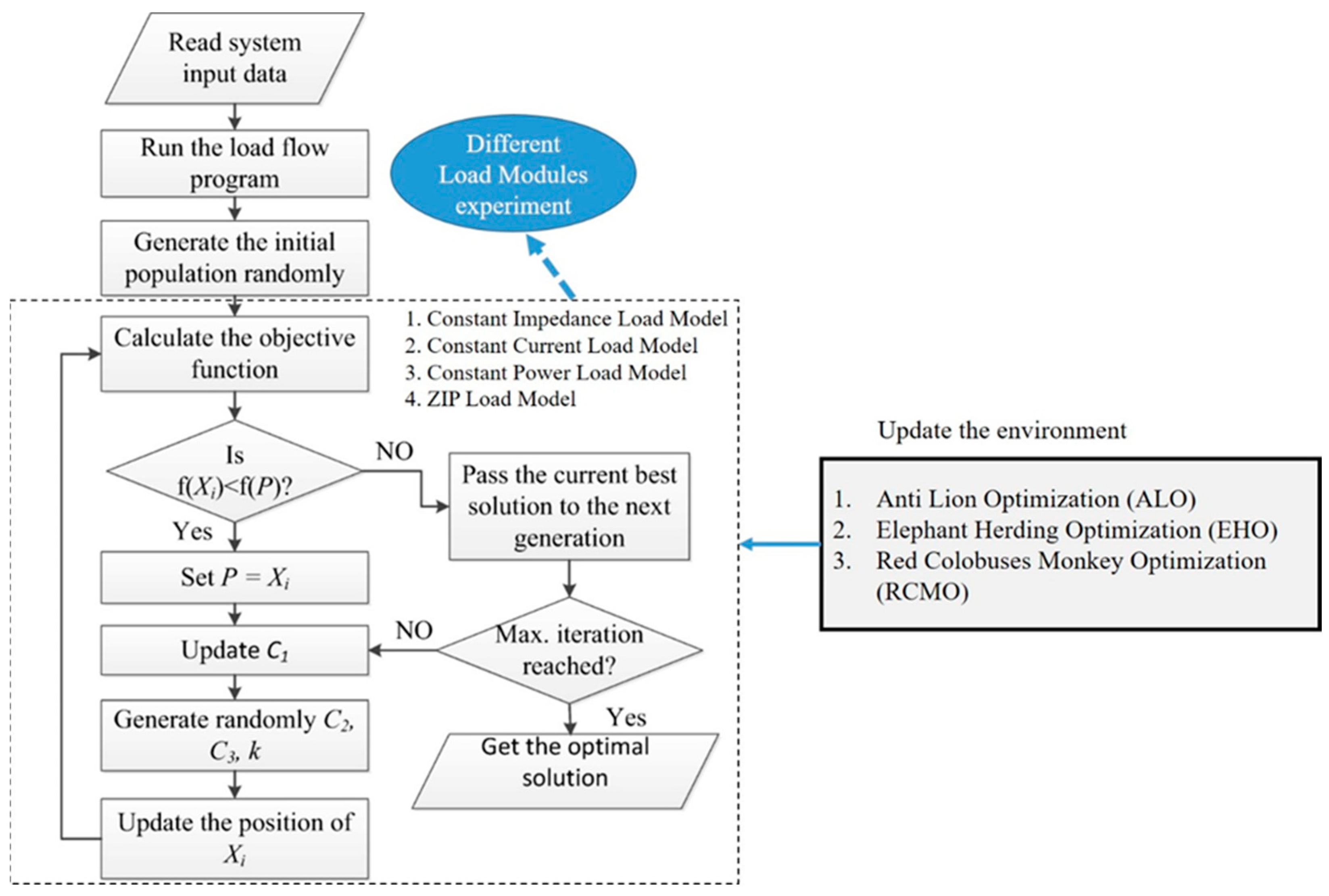This approach leverages three nature-inspired metaheuristic algorithms Red Colobus Monkey [19], Elephant Herding Optimization [20], and Ant Lion Optimization algorithm [21] to solve multiple load models and achieve robust optimization. The major purpose of this methodology is to identify the distribution network plans and sizing of DERs depending on the load characteristics within the distribution network.

The process starts with taking system input data and running the load flow program. It then creates the initial population randomly; it is the optimization algorithms’ origin or beginning point. The optimization process involves calculating each step using objective functions to solve the problem iteratively. If the current solution ($f\left(X_i\right)$) is better than the previous best ($f\left(p\right))$, it is considered the new best solution and is stored in the ‘best’ variable. The algorithm continues to make adjustments and generate new solutions until either the set number of iterations is completed, or the best possible solution is reached. A detailed flowchart of this process is provided in Figure 1.

2.1. Load Modeling in a Power Flow Analysis

The proposed power flow and stability measurements reveal the optimal decisions to improve the system’s performance. Hence, each model of the components that make up the complete power system has to be captured in only one model. In power system analysis, two fundamental models represent loads: static and dynamic models [22]. This is, however, primarily because users are always inclined to go for the simpler, less complex static models. These are simpler to perform since they are characterized by simple mathematical formulas that match load power with voltage and frequency. Static models, which include the constant impedance model, constant current model, ZIP model, and constant power model, are less complex in terms of both computation time and Central Processing Unit (CPU) power; this is more advantageous when dealing with large systems like load flow analysis and contingency analysis [23]. Unlike static models, dynamic models are relatively more sophisticated and utilize differential equations to address the dynamic load profiles [24]. This increases the problem’s dimensionality, and it, therefore, consumes more computation time and power for simulation, which can be a disadvantage, especially for big power systems.

Considering the above-mentioned requirements, our study explores two types of static models: (1) exponential and (2) polynomials for various types of load representation [25]. A crisp detail of both models is given below.

I 

Exponential Representation

The exponential load model represents the active power $P$ and reactive power $Q$ as exponential functions of the voltage magnitude $V$ [26]. The general form of the exponential load model is given by Equations (1) and (2).

$$P=P_0{\left({\displaystyle \frac{V}{V_0}}\right)}^k$$

(1)

$$Q=Q_0{\left({\displaystyle \frac{V}{V_0}}\right)}^m$$

(2)

where $P$ and $Q$ are the active and reactive powers at voltage $V$. $P_0$ and $Q_0$ are the base active and reactive powers at the nominal voltage $V_0$, $k$ and $m$ are the voltage exponents for active and reactive powers, respectively. These exponents typically range from 0 to 2, with k = 1 and m = 1 representing constant power loads and k = 2 and m = 2 representing constant impedance loads.

II. 

Polynomial Representation

The polynomial load model represents the active and reactive powers as polynomial functions of the voltage magnitude [27]. The general form of the polynomial load model is given by Equations (3) and (4).

$$P=P_0\left(a_o+a_1{\left({\displaystyle \frac{V}{V_0}}\right)}^1+a_2{\left({\displaystyle \frac{V}{V_0}}\right)}^2+a_3{\left({\displaystyle \frac{V}{V_0}}\right)}^3+\dots a_n{\left({\displaystyle \frac{V}{V_0}}\right)}^n\right)$$

(3)

$$Q=Q_0\left(b_o+b_1{\left({\displaystyle \frac{V}{V_0}}\right)}^1+b_2{\left({\displaystyle \frac{V}{V_0}}\right)}^2+b_3{\left({\displaystyle \frac{V}{V_0}}\right)}^3+\dots b_n{\left({\displaystyle \frac{V}{V_0}}\right)}^n\right)$$

(4)

where $P$ and $Q$ are the active and reactive powers at voltage $V$. $P_0$ and $Q_0$ are the base active and reactive powers at the nominal voltage $V_0$, $a_0$ and $b_0$ are the coefficients of the polynomial terms for active and reactive powers, respectively, and $n$ is the degree of the polynomial.

Both models provide greater flexibility and can represent a wider range of load behaviors by appropriately choosing the polynomial coefficients.

2.2. Load Models

The details of all four types of load models are discussed below.

I. 

Constant Impedance Model

The constant impedance load model is one of the basic models created for power system analysis. It assumes that the load has a constant impedance nature, which, in other words, indicates that the load’s voltage-to-current ratio is fixed and is not altered by voltage changes [28]. However, this model is quite useful when determining the primary level of electrical loads when subjected to varying voltage parameters.

The impedance $\left(Z\right)$ of a load is represented in terms of resistance $\left(R\right)$ and reactance $\left(X\right)$ and can be calculated according to Equation (5).

$$Z=R+jX$$

(5)

where $R$ is the resistance (in ohms), $X$ is the reactance (in ohms), and $j$ is the imaginary unit ($j^2=-1)$. For the constant impedance model, the impedance can be calculated using Equation (6).

$$Z\left(s\right)=Z_o$$

(6)

where $Z_o$ is a constant impedance.

II. 

Constant Current Load Model

In the constant current load model, the load draws a constant current. $I$ from the system irrespective of the voltage applied. However, current $I\left(s\right)$ varies to maintain a constant current [29]. For the constant current model, the current can be calculated using Equation (7).

$$I\left(s\right)=I_o$$

(7)

where $I_o$ is a constant current.

III. 

Constant Power Load Model

The constant power load model consumes a constant amount of power $P$ from the system, adjusting its power to maintain this power consumption [30]. Here, power $P\left(s\right)$ varies to maintain constant power and can be calculated using Equation (8).

$$P\left(s\right)=P_o$$

(8)

where $P_o$ is a constant power.

IV. 

ZIP Load Model (Impedance, Current, Power)

The ZIP load model comprises constant impedance ($Z\left(s\right)$), constant current ($I\left(s\right)$), and constant power ($P\left(s\right)$) to look closer at real-life load applications in the power system [31]. It is typically represented with combinations of polynomial or piecewise functions for each component.

2.3. Fitness Function

Our fitness function $f\left(x\right)$ incorporates the optimal positioning and sizing of capacitors (C), battery systems (BSs), solar panels (PVs), and wind turbines (WTs). This fitness function aims to minimize costs, losses, and voltage deviations while maximizing renewable energy utilization as defined in Equation (9).

$$minf\left(x\right)=w_1\ast C_{loss}+w_2\ast P{V}_{loss}+w_3\ast B{S}_{loss}+w_4\ast W{T}_{loss}$$

(9)

where $C_{loss}$ is the cost associated with reactive power losses in capacitors, $P{V}_{loss}$ is cost related to active power loss in solar panels, $B{S}_{loss}$ and $W{T}_{loss}$ refer to active power loss in battery systems and wind turbines, respectively. Moreover, $w_1,$ $w_2,$ $w_3,$ and $w_4$ are weight parameters used to balance different components of a multi-objective optimization problem given in Equation (9). Mathematically, ${{\displaystyle \sum }}_{i=1}^4{w}_i$ = 1.

2.4. Mathematical Modeling of Distributed Components

2.4.1. Solar Photovoltaic (SPV)

Solar photovoltaic (SPV) is an important component of our designed distributed system. SPV panels are inclined at an angle equal to the latitude of the considered area to increase the amount of solar radiation received on the SPV surface. The electrical power output of an inclined SPV system mainly depends on the amount of beam radiation and diffuse radiation falling on the SPV surface. The total hourly solar radiation [32] on a fixed inclined surface (HT) can be calculated according to Equation (10).

$$H_T=H_b{R}_b+H_d{R}_d+\left(H_b+H_d\right)\ast R_{\tau }$$

(10)

where H_T is in kWh/m², H_b is the beam part of solar radiation (kWh/m²), H_d is the diffused part of solar radiation (kWh/m²), R_b is the tilt factors for beam radiation, R_d is the tilt factors for diffused radiation, and R_r is the tilt factor for reflected part of solar radiations. The hourly power output of the SPV system (P_SPV) [32] is calculated from Equation (11).

$$P_{SPV}=\eta H_{T}A$$

(11)

where η is the conversion efficiency of the SPV system, and A is the surface area of the SPV system. The annual energy output [32] of the SPV system is estimated using Equation (12).

$$E_{SPV}={{\displaystyle \sum }}_{i=1}^{8760}{P}_{SPV}\left(i\right)$$

(12)

2.4.2. Wind Turbine

Wind speed continuously varies at a particular site. It depends on the local land terrain, weather system, and height above the ground. Therefore, it is necessary to capture wind speed variation in a model to forecast energy production. The Weibull probability density function best describes the wind speed variation. The Weibull probability density function [32] of wind speed (V) is defined in Equation (13).

$$\mathrm{f}\left(\mathrm{V},\mathrm{k},\mathrm{c}\right)=\left({\displaystyle \frac{k}{c}}\right){\left({\displaystyle \frac{V}{c}}\right)}^{k-1}\exp \left[-{\left({\displaystyle \frac{V}{c}}\right)}^k\right]$$

(13)

where f(V,k,c) is the probability of wind speed (V), c is the scale parameter, k is the shape parameter, and V ≥ 0, k > 1, c > 0. The output of a wind energy system depends on the rated power (Pr) of the wind turbine, cut-in speed, cut-out speed, and rated speed. Mathematically, the electrical power output of a wind turbine (PWT) is calculated using Equation (14).

$$P_{WT}=\left\{\begin{array}{c}0 0\le V< V_{cut\text{-}in} and V>V_{cut\text{-}out}\\ a V^3+b{P}_r V_{cut\text{-}in}\le V<V_{rated}\\ P_r V_{rated}\le V\le V_{cut\text{-}out} \end{array} \right\}$$

(14)

where V_cut-in is the cut-in speed, V_cut-out is the cut-out speed, V_rated is the rated speed of the wind turbine. Constants a and b are functions of the rated speed and cut in speed of the wind turbine and calculated using Equations (15) and (16).

$$a={\displaystyle \frac{P_r}{V_{rated}^3-V_{cut\text{-}in}^3}}$$

(15)

$$b={\displaystyle \frac{V_{cut\text{-}in}^3}{V_{rated}^3-V_{cut\text{-}in}^3}}$$

(16)

The annual energy production (E_WES) from a wind turbine at a specific site can be estimated using Equation (17).

$$E_{WES}=365\ast 24\ast {\displaystyle \sum }_{V=0}^{V_{cut\text{-}out}}{P}_{WT}\ast \mathrm{f}\left(V,k,c\right)$$

(17)

At a given hub height, the wind speed can be calculated by following the power-law relation defined in Equation (18).

$$\left({\displaystyle \frac{V}{V_r}}\right)={\left({\displaystyle \frac{h}{h_r}}\right)}^n$$

(18)

where $V$ and $V_r$ are the wind speed at the hub height ‘h’ and the reference height ‘hr’, and n is the power-law exponent (1/7).

2.4.3. Capacitor Bank

A capacitor bank is an assembly of capacitors connected in series and/or parallel to obtain the required capacitance and voltage. When placed on the system, the main use of capacitor banks is to provide reactive power that enhances the voltage characteristics, thus minimizing losses. The basic relationship between the capacitance C of a capacitor bank and the supplied reactive power $Q_c$ is defined in Equation (19).

$$Q_c=V^2\omega C$$

(19)

where

• $Q_c$ is the reactive power supplied by the capacitor bank;
• $V^2$ is the voltage across the capacitor bank (in volts);
• ω is the angular frequency of the system (ω = 2πf, where $f$ is the frequency in Hz);
• C is the capacitance of the capacitor bank (in farads).

For capacitor banks with capacitors connected in parallel and series [33], the equivalent capacitance $C_{eq}$ can be calculated using Equations (20) and (21).

$$\mathrm{For}\mathrm{parallel}\mathrm{mode}:C_{eq}={{\displaystyle \sum }}_{i=1}^n{C}_i$$

(20)

$$\mathrm{For}\mathrm{series}\mathrm{mode}:{\displaystyle \frac{1}{C_{eq}}}={{\displaystyle \sum }}_{i=1}^n{\displaystyle \frac{1}{C_i}}$$

(21)

where

• $C_i$ is the capacitance of the $i^{th}$ capacitor;
• $n$ is the number of capacitors.

2.5. Metaheuristic Algorithms

The induced energy management problem in DG systems is optimized using three metaheuristics: (1) Ant Lion Optimization, (2) Elephant Herding Optimization, and (3) Red Colobus Monkey Optimization algorithms. A crisp description of these algorithms is given below.

I. 

Ant Lion Optimization

Ant Lion Optimization (ALO) is a popular metaheuristic algorithm based on the hunting mechanism of antlions, developed by Seyedali Mirjalili [21]. This algorithm simulates the interaction between ants and antlions when hunting and running away. The work of conventional ALO is discussed below.

• Population initialization: Ants in this algorithm represent an initial population of solutions on a search landscape. Each ant’s position is kept in a vector in the manner described below:

$$\mathrm{Position}\mathrm{of}\mathrm{Ants}:\mathrm{A}=[A_1, A_2,\dots A_N]$$

$$\mathrm{Position}\mathrm{of}\mathrm{Antlions}:\mathrm{L}=[L_1, L_2,\dots L_N]$$

where for $j^{th}$ iteration, $A_i$ and $L_i$ are calculated using Equations (22) and (23).

$$A_i^j=l{b}^j+\left(u{b}^j-l{b}^j\right)\ast rand \left(0,1\right)$$

(22)

$$L_i^j=l{b}^j+\left(u{b}^j-l{b}^j\right)\ast rand \left(0,1\right)$$

(23)

where $i\in \left(1,2,\dots ,N\right)\mathrm{and}j\in \left(1,2,\dots ,D\right)$.

Here, each ant and antlion’s position is randomly initialized within the search space boundaries [lb,ub].

• Random walk of ants: the random walk of ants is modeled according to the following stochastic process:

$$RW\left(t\right)=\left[0, cumsum \left(2.r\left(t_1\right)-1\right), cumsum \left(2.r\left(t_2\right)-1\right), \dots ,cumsum \left(2.r\left(t_n\right)-1\right)\right]$$

where $cumsum$ is the cumulative sum, $r\left(t_i\right)$ is a random number in [0,1], and $n$ is the number of steps. The position of the ants after the random walk is normalized within the search space boundaries according to Equation (24).

$$A_i\left(t+1\right)=lb+\left(R{W}_i\left(t\right)+R{W}_i^{min}\right)\ast {\displaystyle \frac{ub-lb}{R{W}_i^{max}-R{W}_i^{min}}}$$

(24)

• Trapping in antlion’s pit

Each ant is influenced by an antlion using Equation (25).

$$A_i\left(t+1\right)={\displaystyle \frac{R{W}_i\left(t\right)+R{W}_e\left(t\right)}{2}}$$

(25)

where $R{W}_e\left(t\right)$ is a random walk around the elite solution.

• Adaptive boundaries

The boundaries for the random walk are adaptively adjusted using Equations (26)–(28) for the current iteration t

$$I=10\ast {\displaystyle \frac{t}{T}}$$

(26)

$$l{b}_i\left(t+1\right)=l{b}_i\left(1-{\displaystyle \frac{I}{T}}\right)$$

(27)

$$u{b}_i\left(t+1\right)=u{b}_i\left(1-{\displaystyle \frac{I}{T}}\right)$$

(28)

where $T$ indicates the maximum number of iterations.

• Fitness function

The fitness of each ant and antlion is computed using the objective function $f\left(.\right)$ defined in Equations (29) and (30).

$$F_{A_i}=f\left(A_i\right)$$

(29)

$$F_{L_i}=f\left(L_i\right)$$

(30)

• Selection and update

The position of an antlion is updated if an ant trapped in its pit has better fitness as defined in Equation (31).

$$L_i=A_i if F_{A_i}<f\left(A_i\right)$$

(31)

The elite antlion (best solution) is updated according to Equation (32).

$$L_{elite}=A_j if F_{A_j}<f\left(L_{elite}\right)$$

(32)

II. 

Elephant Herding Optimization

Elephant Herding Optimization (EHO) is a metaheuristic optimization algorithm inspired by the social behavior of elephants in a herd [20]. Originally, elephants reside in herds, which are grouped in clans, and each clan has its own matriarch—the oldest and most knowledgeable female elephant. The division of herds into clans and the movement of elephants towards the matriarch’s leadership is the core of the EHO algorithm. The algorithm models the behavior of elephants in terms of two main phases: (1) clan updating operation and (2) separating operator.

The clan updating operation is the procedure of updating the positions of elephants within a clan. Every elephant optimizes its location according to the matriarch position (the best solution in the clan) and the mean position of all the elephants in the clan. Mathematically, the new position of an elephant in dimension $j$ at time $t+1$ is calculated using Equation (33).

$$x_{i,j}\left(t+1\right)=x_{mean, i,j}\left(t\right)+\alpha \ast r\ast \left(x_{best, i,j}\left(t\right)-x_{i,j}\left(t\right)\right)$$

(33)

Here, $x_{i,j}\left(t\right)$ represents the current position of elephant $i$, while $x_{best, i,j}\left(t\right)$ is the position of the matriarch in the same clan. The parameter α is a scale factor that determines the impact of the matriarch’s position where r is a random number between 0 and 1 for the purposes of stochasticity. This process enables the elephants to make a transition towards this best-known solution while at the same time keeping the population as diverse as possible. The second stage, called the separating operator, seeks to guarantee that the worst-performing elephants are relocated to random positions in the search space. It avoids trapping the algorithm within local optima which leads the search in random directions of the search space. Mathematically, the position of the worst elephant in the population is updated using Equation (34).

$$x_{worst,j}\left(t+1\right)=rand \left(L_j,U_j\right)$$

(34)

In this Equation, $L_j and U_j$ refers to the lower and upper bound of the search space at each dimension.

III. 

Red Colobus Monkey Optimization

Red Colobus Monkey Optimization, abbreviated as RCMO, is an evolutionary optimized algorithm in the context of the social behavior of Red Colobus Monkeys. The algorithm emulates how monkeys search for food and signal to other members of the same group to help find solutions to optimization problems [19]. Below are the key mathematical concepts.

• Population initialization

Each monkey represents a candidate solution, initialized using Equation (35).

$$x_i=L_j+r_j\ast \left(U_j-L_j\right)$$

(35)

where $L_j$ and $U_j$ are the lower and upper bounds, respectively, and $r_j$ is a random number between 0 and 1.

• Leader selection

The best-performing monkey in each group becomes the leader by minimizing the fitness function defined in Equation (36).

$$x_{leade{r}_k}=\arg \min f\left(x_i\right)$$

(36)

• Position update (exploitation)

Monkeys update their positions based on the leader calculated by Equation (37).

$$x_i\left(t+1\right)=x_i\left(t\right)+\beta \ast r_1\left(x_{leade{r}_k}\left(t\right)-x_i\left(t\right)\right)+\gamma \ast r_2$$

(37)

where $\beta$ controls leader influence, $\gamma$ adds random exploration, and $r_1$, and $r_2$ are random numbers.

• Global communication (exploration)

Monkeys communicate across groups to refine their search according to Equation (38).

$$x_i\left(t+1\right)=x_i\left(t\right)+\delta \ast r_r*(x_{best}-x_i\left(t\right))$$

(38)

• Balancing exploration and exploitation

Dynamic adjustments between exploration and exploitation using Equation (39).

$$\beta \left(t\right)={\beta }_0\ast \left({\displaystyle \frac{\left(T-t\right)}{T}}\right)$$

(39)

where T is the total iterations and ${\beta }_0$ is the initial value.

• Termination

The algorithm terminates when the fitness change is small enough according to Equation (40).

$$\parallel f\left(x_{best}\left(t+1\right)\right)-f\left(x_{best}\left(t\right)\right)\parallel <\epsilon$$

(40)

3. Proposed Methodology

The main problem solved in this paper lies in identifying the size and location of the RESt distribution system, given that the system’s total cost must be minimized while satisfying the constraints. The minimization of the total losses of the distribution system, cost of the PV units, cost of wind turbines, capacitors, and battery systems is considered under this factor. Other technical constraints include load balance constraints, voltage, power flow limits, irradiance/wind speed limit cost variations in respective underestimated and overestimated histograms, and the amount of power that can be supplied from the DG units. To compute these factors, we implemented the Monte Carlo simulation on PV and wind turbines for cost analysis and to determine uncertainties in the parameters such as solar irradiance and system performance. The proposed technique involves generating random samples of input parameters, evaluating corresponding costs, and estimating the results to determine optimal solutions. Our methodology consists of two cases: (1) determining the size and location of all four components (PV, WT, battery, capacitor), and (2) the cost estimation with varying atmospheric conditions (with fixed size and location of battery and capacitor).

3.1. Cost of PV and Wind Turbines Units

The Monte Carlo optimization method, however, is a powerful stochastic technique that can be used for the cost analysis of PV and wind turbine systems incorporating real uncertainties in parameters such as solar irradiance, wind flux, and system efficiency. It includes selecting random input parameters and evaluating costs associated with the generated data for efficient solutions.

3.1.1. Parameters and Setup

In the early phase, the parameters for Monte Carlo optimization are initialized according to

Table 1. Parameter initialization for PV and wind turbine simulation using Monte Carlo optimization.

Parameters	For PV Environment	For Wind Turbines Environment
Number of trials (N)	100,000	100,000
Cost due to underestimation (CU)	300 $/MW	300 $/MW
Cost due to overestimation (CO)	700 $/MW	700 $/MW
Dispatched power (Ws)	1.6 MW	0.8 MW

. The standard underestimation and overestimation cost parameters are adapted from the article [34].

Here, cost due to underestimation (CU) represents the cost incurred to use expensive conventional power instead of cheaper renewable energy when the actual generation is higher than expected. Cost due to overestimation (CO) is the cost incurred through backup or reserve power when the forecasted renewable generation is unnecessarily higher than actual generation to stabilize the grid, leading to higher operating expenses. Dispatched power (Ws) is the generated renewable energy, sanctioned by projected generation, power requirement, or storage availability. In this experiment, the power generated by the PV system $W\left(i\right)$, is calculated by following equations based on the irradiance $G\left(i\right)$. These equations are adapted from the article [32].

$$W\left(i\right)=\left\{\begin{array}{c}{P}_{sr} \left({\displaystyle \frac{G{\left(i\right)}^2}{G_{std}\ast R_c}}\right) if 0<G\left(i\right)<R_c\\ P_{sr} \left({\displaystyle \frac{G\left(i\right)}{G_{std}}}\right) if G\left(i\right)\ge R_c \end{array}\right\}$$

(41)

where $P_{sr}$ is the rated power, $G_{std}$ is the standard irradiance, and $R_c$ is the cut-off irradiance [35,36]. For each iteration, we compared the dispatched power ($W_s)$, to the generated power $W\left(i\right)$. If the dispatched power exceeds the generated power, then the cost due to overestimation ($CO$) is calculated using Equation (42) otherwise the cost due to underestimation ($CU$) is evaluated using Equation (43).

$$CO\left(i\right)=\left\{\begin{array}{c}CO\ast \left(W\left(s\right)-W\left(i\right)\right) if W\left(s\right)>W\left(i\right)\\ 0 Otherwise\end{array}\right\}$$

(42)

$$CU\left(i\right)=\left\{\begin{array}{c}CU\ast \left(W\left(s\right)-W\left(i\right)\right) if W\left(s\right)>W\left(i\right)\\ 0 Otherwise\end{array}\right\}$$

(43)

3.1.2. Random Generation and Cost Estimation of Wind Turbine

In the wind turbine, the relationship between the wind parameters (shape ($k$), scale ($c$)) and produced wind speed ($V$) can be defined according to Equation (44) [32].

$$V\left(i\right)=wblrand\left(c,k\right)$$

(44)

where $wblrand$ is the randomized Weibull distribution of the wind parameters. Further, the power produced by the wind turbine $w\left(i\right)$ [32] is computed by wind speed $V\left(i\right)$ and the wind turbine’s power is defined in Equation (45).

$$W\left(i\right)=\left\{\begin{array}{c}0 if V_i<V_r or V_i> V_0\\ a V\left(i\right)+b V_i\le V\left(i\right)<V_r\\ W_r V\left(i\right) \ge V_r \end{array} \right\}$$

(45)

Here, where $V_i$ is the cut-in wind speed, $V_0$ is the cut-out wind speed, $V_r$ is the rated wind speed, $W_r$ is the rated power, and $a$ and $b$ are coefficients for the linear region of the power curve [37]. Similarly to PV, the dispatched power Ws are compared with the generated power $W\left(i\right)$. If the dispatched power exceeds the generated power, calculate the cost due to overestimation (CO) using Equation (42). Otherwise, if the generated power exceeds the dispatched power, calculate the cost due to underestimation (CU) using Equation (43).

3.2. IEEE 33 Bus System

The IEEE 33 Bus Test System is important in power system engineering as a benchmark for testing and validating many algorithms and techniques required to examine, analyze, optimize, and protect distribution systems [38]. It defines the load distribution on the buses and contains the buses with residential, commercial, and industrial loads. Every bus has a certain load demand in kW and kVAR, which is determined for each bus individually. The system consists of 33 buses that can be regarded as nodes through which power flows in or out of the system or along which power can be shared (Figure 2). These buses are linked by 33 branches or lines that regulate the supply of electrical energy between the buses. It provides or delivers the needed electrical energy transmitted through the electricity network. It also comprises forty-eight loads spread on the buses 2–33. They also incorporate 32 loads, known as buses, which spread from 2 to 33. These loads model the demand for electrical power in the network, and their distribution is important for analyzing the system’s response under different kinds of loads.

3.3. Essential Strategies for Optimizing

It is known that a system that minimizes losses is also more reliable, ensuring a stable and consistent energy flow that enhances overall performance and maintains service quality without interruptions. When comparing different optimization strategies, it is essential to evaluate loss reduction by assessing how each algorithm minimizes power losses across the entire system, including components like solar panels, wind turbines, capacitors, and energy storage systems. In this context, the detailed performance of all three metaheuristic algorithms (Section 2.5) is discussed in the subsequent subsections.

3.3.1. Optimization Using ALO Algorithm

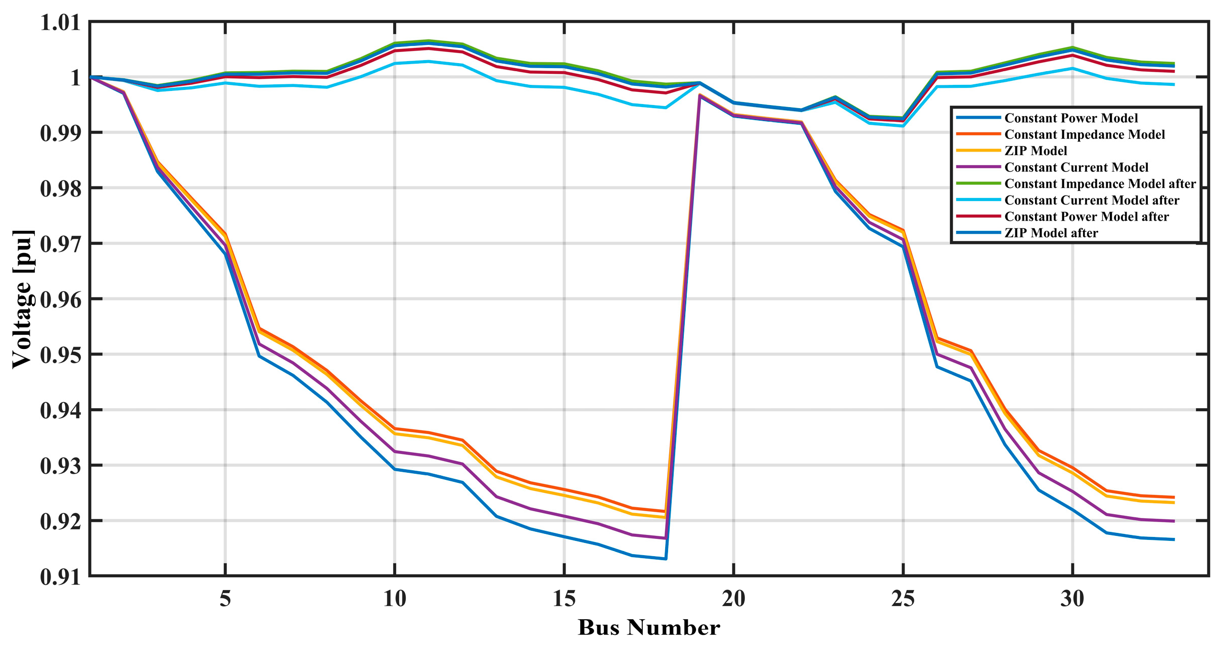
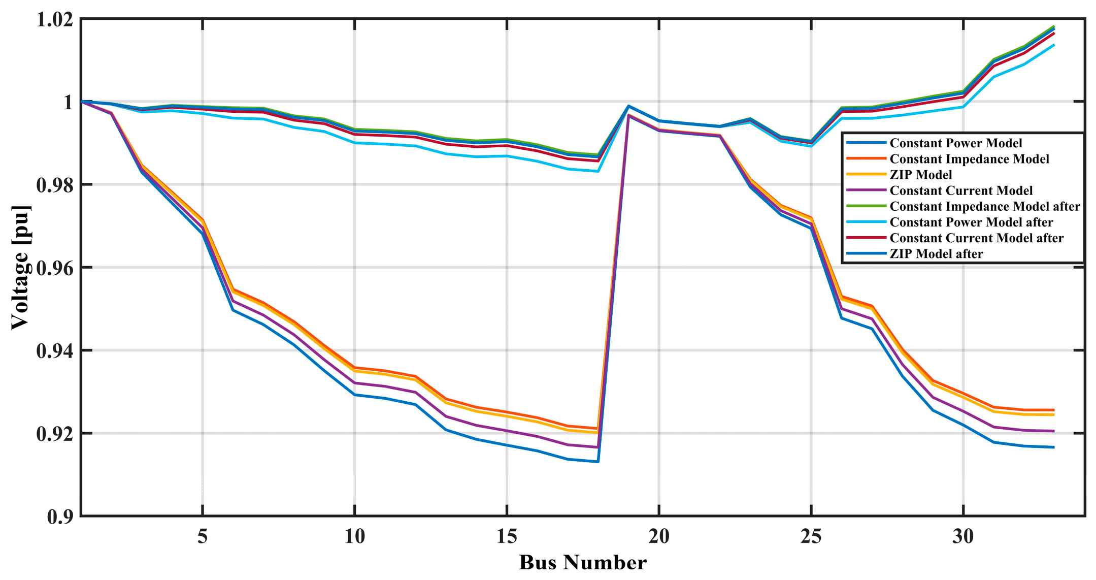
Initially, four load models: (1) constant power, (2) ZIP, (3) constant impedance, and (4) constant current, were implemented to generate respective voltage profiles. Each load type exhibits distinct characteristics under different voltage conditions. The voltage profile graph in Figure 3 illustrates the voltage profiles before and after optimization using the Ant Lion Optimization (ALO) algorithm for four different load models: The four most commonly used residential load models are namely the constant power model, ZIP model, constant impedance model, and constant current model. Specifically, the voltage profiles before optimization are characterized by steep declines between buses 1 and 18 and buses 20 and 35, which show that voltage deviations with steep slopes are quite significant; this conclusion especially applies to the constant power and the constant current models. These steep dips indicate regions demonstrating that the voltage simulates to a lower value, and the steep rise in the curve, which denotes the bus number 20, results from a certain action or generation point.

From the analysis above, after optimization, the voltage profiles for all the models have fewer steep slopes and considerably reduced voltage drops across all the buses, portraying better voltage regulation. As with the optimized profiles, the curves are less steep, and there are not many spikes and spikes in voltage; around bus 20, the voltage gradually changes to the peak. By analyzing the constant power model, it is possible to observe a highly enhanced voltage stability in the network after the optimization is realized, where the voltage stays close to 1. The ZIP and constant impedance models provide rather smooth and stable voltage fluctuations. At the same time, the constant current model also demonstrates a rather marked qualitative improvement of the voltage profile after its optimization is performed.

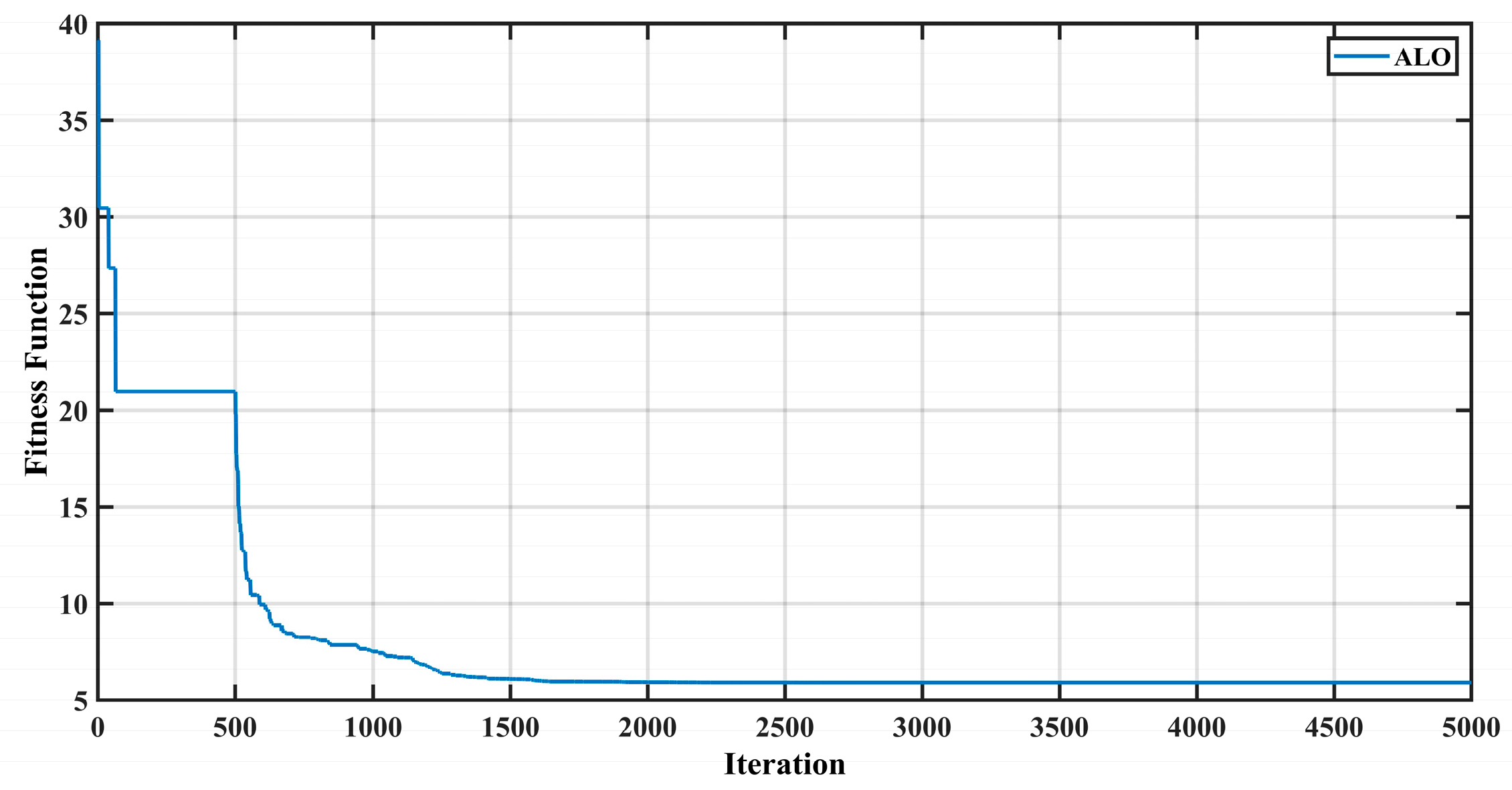
The convergence graph (Figure 4) depicts the ALO algorithm’s fitness function at different bus numbers, showing how the algorithm performs at reducing the fitness function. The fitness function represented on the y-axis is the goal that the ALO aims for the algorithm; in the terminology of power systems, it includes optimizing power losses, improving the voltage profile, or deciding on the location and capacity of capacitors, PV systems, wind turbines, and batteries. The y-axis, titled “Cost”, is probably the measure of the iteration steps or the degree of buses connected to the power system under consideration. Each step coincides with the iteration through the optimization techniques, where the algorithm evaluates and adjusts the solution. Analyzing the graph, it can be noted that the overall trend decreases steeply at the beginning. This allows for the ALO algorithm to find a pretty good approximation of the solution quickly. After this sharp first drop, the curve relatively levels off, thus indicating that the algorithm is approaching a near-optimal or an optimal solution. The flat segment of the curve suggests that any extra iterations are not improving the solution much; hence, the algorithm has successfully converged. The sharp decline at the beginning of the graph shows that the ALO algorithm can converge on a solution that is comparatively good in minimal time. The cruder steps in the subsequent iterations are better than the previous one and imply that the algorithm is fine-tuning to become closer to the optimal solution. This is the final level of the algorithm that shows that the solution found is optimal; any attempts to add other values will result in negligible changes. Therefore, the convergence graph proves the applicability of the Ant Lion Optimization in solving real power systems problems, for which there are several components to consider, as well as different load models.

3.3.2. Optimization Using EHO Algorithm

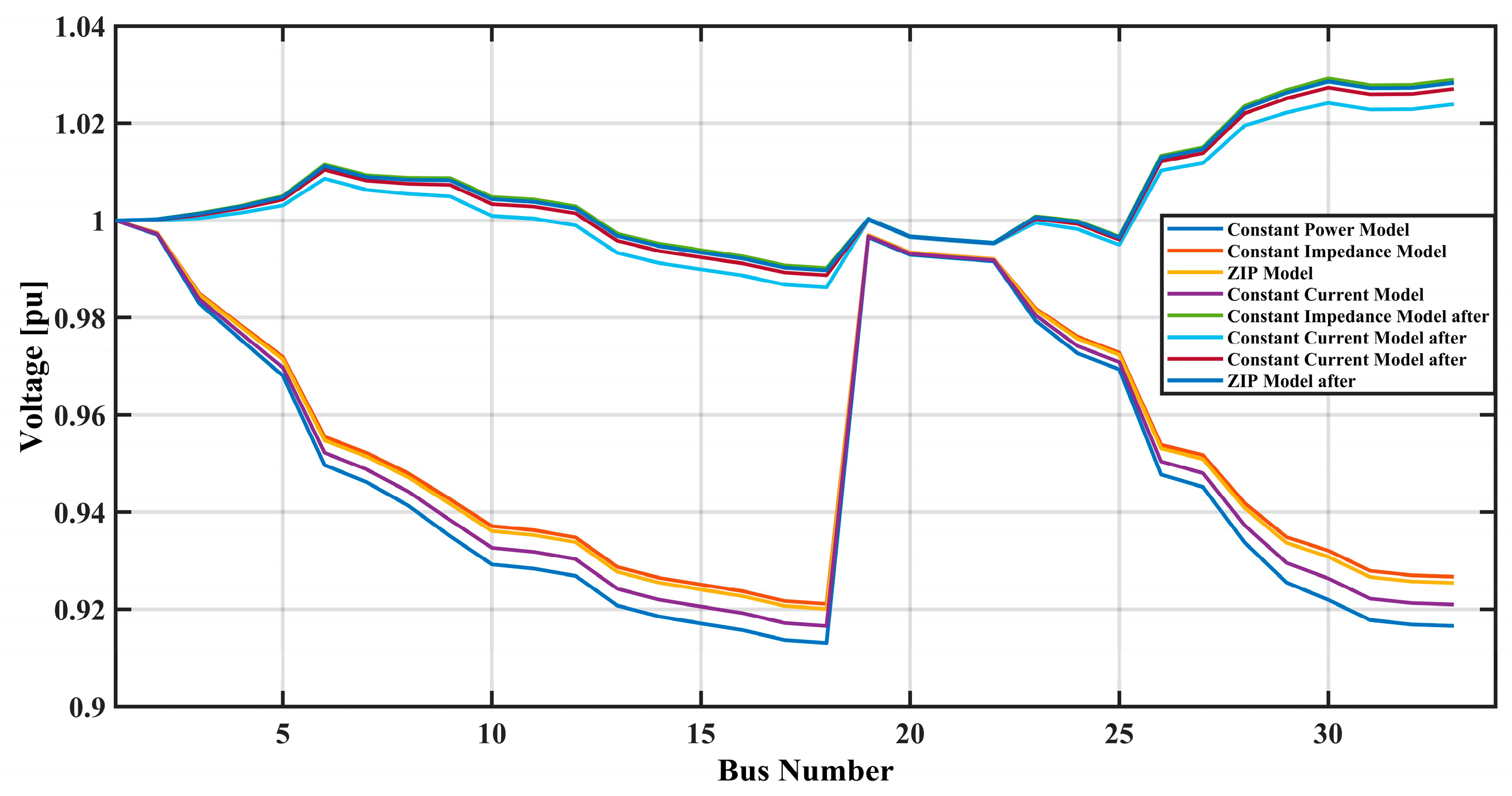
The voltage profile graph in Figure 5 shows how the optimization of the IEEE 33 Bus System using the EHO has affected the improvement. This optimized technique called the EHO algorithm is an elegant stimulus for optimization that is derived from the habits of elephant groups. They are socially organized in a matriarchal system, and the largest and oldest female in the group is the matriarch. This algorithm is based on the hierarchy and cooperative behavior of the herds of elephants for the exploration and exploitation of the search space in the problems of optimization. The voltage profile before and after optimization is presented for all the load models. As shown, before the optimization of the network, the voltage deviations are higher, and the values are depicted for buses with high numbers to reveal voltage drops. These deviations are essential as they result in the ineffective use of energy in the network and possible instabilities. Thus, when applying the EHO algorithm, one can observe that the voltage profile is much better. It includes a step-by-step augmenting and reducing of certain quantities controlling the voltage level of the power system, for instance, transformers tap settings, the amount of capacitive var support supplied by capacitor banks, and other controlling variables. The obtained results indicate that the voltage levels are regulated to a greater extent and are closer to the ideal value of 1 pu. It implies that the improvement is even more noticeable in areas where there were steep voltage drops before the use of optimization techniques.

Technically, the updating process employed within the EHO algorithm takes a clan-based structure, with each clan’s solutions affected by its matriarch, as defined in Equations (33) and (34). The position of each solution (elephant) in the search space is adapted according to the position of the best solution (matriarch) within the clan. Furthermore, a separating operator prevents a change in position of the mutant and trial vector in the whole population by resting it randomly in the problem space. Since the EHO algorithm balances exploration and exploitation, a search for the optimal or near-optimal solution is possible.

The convergence graph in Figure 6 shows the quality of EHO in solving the fitness function for several iterations. In this regard, the fitness function is an indication of the algorithm’s goal, which includes the reduction in power losses, the enhancement of voltage profiles, or the proper installation and ratings of equipment, including capacitors, PV systems, wind turbines, and battery energy storage systems in a power system. The abscissa axis is “Iterations”, meaning the number of times the EHO algorithm has run. Every iteration is related to a step of the optimization process during which the solution is assessed and adjusted. The y-axis refers to the “Fitness Function” value at each iteration. The curve drops at a sharp initial point: the EHO algorithm obtains one good solution very rapidly; then, the graph runs steeply down until nearly leveling off, giving insight that the algorithm was approximately approaching an optimal solution point. The flat point refers to the minimal gain within further iterations, referring towards convergence. The initial spiky and slowly oscillating spikes indicate a good convergence of the algorithm during fine-tuning, whereas the last flat stage denotes minimal variations due to iteration, further establishing the satisfactory convergence of the algorithm toward a solution.

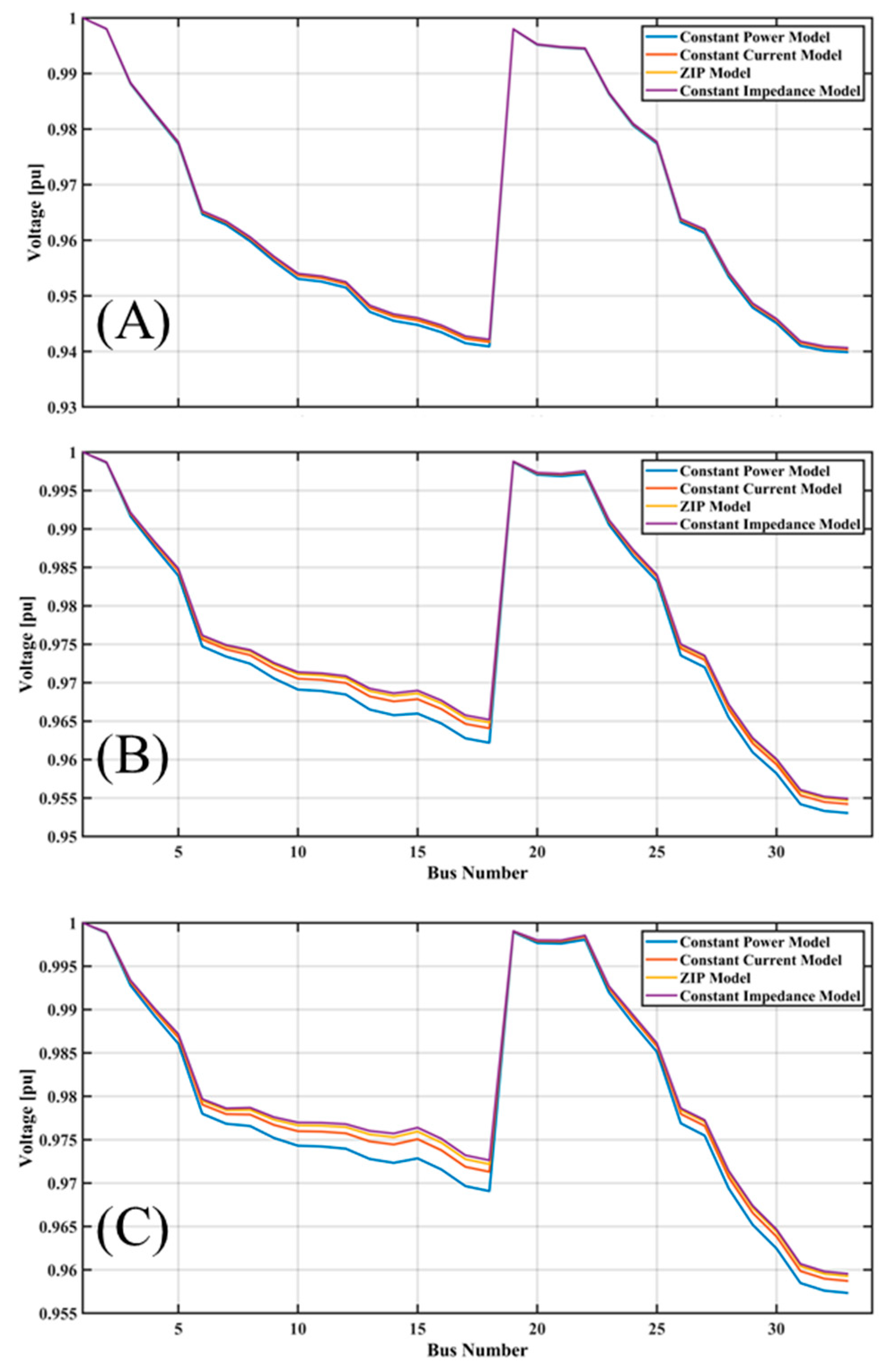
3.3.3. Optimization Using RCMO Algorithm

The graph shown in Figure 7 represents the voltage profile for the four load models as a part of the IEEE 33 Bus system before and after applying the Red Colobus Monkey Optimization Algorithm. This graph shows the voltage profile for different bus numbers in a power distribution network for the different load models, including constant power, constant impedance, constant current, and ZIP, a combination of all these models. The comparison between the pre-optimization and post-optimization levels of voltage is an excellent way to illustrate the energy management strategies’ impact on improving grid stability and efficiency. Before optimization, the voltage drops at all the load numbers are quite high in general, especially in the load-demanding areas or even weaker supply areas. The impedance model is characterized by the highest rate of decline and, therefore by the highest sensitivity to a change in loads. A pattern like this shows that the network is unstable with inefficiencies under preoptimized conditions. After optimization, the voltage profiles improve greatly for all the models, where higher and more stable values are seen across most of the bus numbers. For the ZIP model, which is one of the realistic load conditions by combining constant power, current, and impedance effects, notable improvements in the voltage levels are seen. The optimization reduces the dips in the voltage, mainly at critical buses with the highest demand for loads, thus leading to a relatively uniform and stable voltage profile. The sharp increase seen near certain buses, for example, near bus 20, is indicative of the existence of power injection sources, such as distributed generation or capacitor banks, which help in voltage stability. The overall flattening of the voltage profile after optimization shows that the system is well-balanced, and this is essential for the maintenance of power quality and the minimization of energy losses. This shows that the optimization process is effective in enhancing the reliability and performance of distributed renewable generation and storage systems.

Figure 8 displays the graph of an initial constant fitness phase followed by a steep rise as the algorithm nears the solution. Later, declines in fitness values point to qualitative improvements, and the algorithm explores and exploits the solution space. Oscillations correspond to the search and refinement of the algorithm, with which the value of the fitness function diminishes gradually. The last steady section indicates that it converges to the optimal or near-optimal solution, where sharp oscillations are followed by stabilization; therefore, the RCMO algorithm is successful in solving complicated optimization problems in power systems.

3.4. Mathematical Uncertainty Estimation Using Monte Carlo Simulation

Monte Carlo implementation comprises statistical testing to compute the cost of a designed distributed network by utilizing random sampling. In the context of renewable energy systems, various test cases were designed using lognormal distribution sampling for irradiance and Weibull sampling of wind power. The details of the parameters are given in

Table 2. Details of initial parameters for photovoltaic and wind power systems used in the simulation.

Photovoltaic Parameters and Their Description
Parameter	Description	Value
Rated Power Output (Psr)	Power output capacity of the PV system	65 MW
Standard Irradiance (Gstd)	Benchmark solar irradiance level	1000 W/m2
Critical Irradiance (Rc)	Threshold solar irradiance for PV operation	150 W/m2
Maximum Power (Wmax)	Upper limit of PV system output	2 MW
Solar Irradiance (G)	Modeled solar irradiance distribution	Lognormal (λ = 6, β = 0.25)
Wind Power System Parameters
Cut-in Wind Speed (Vi)	Minimum wind speed for turbine operation	4 m/s
Rated Wind Speed (Vr)	Wind speed for nominal turbine output	10 m/s
Cut-out Wind Speed (Vo)	Maximum safe operating wind speed for turbines	15 m/s
Rated Power Output (Wr)	Power output capacity of the wind turbine	1 MW
Weibull Scale Parameter (c)	Derived from Rayleigh distribution	$\sqrt{2}$ σ (σ = 7.5 m/s)
Weibull Shape Parameter (k)	Shape factor for Weibull wind speed distribution	2
Cost Parameters
Cost due to Underestimation (Cu)	Penalty for under-forecasting power generation	$30/MW
Cost due to Overestimation (Co)	Penalty for over-forecasting power generation	$70/MW

. Further, for each sample of weather data, the energy generated by the photovoltaic solar and wind systems, is calculated by using the following mathematical formulas defined in Equations (46) and (47).

$$P_{solar}=A\cdot E\cdot \eta$$

(46)

$$P_{wind}=0.5\ast \mathsf{\rho }\ast A\ast v^3\ast \eta$$

(47)

where A is the area (for solar panels or turbine blades), E is the solar irradiance or wind speed, ρ is the air density, v is wind speed, and η is efficiency. Further, the costs due to underestimation and overestimation are calculated according to Equations (48) and (49), respectively.

$$\mathbf{Underestimation}\mathbf{cost}:C_{under}={{\displaystyle \sum }}_{i=1}^N\left(Forcas{t}_i-Actua{l}_i\right)\ast C_{Penalty, under}$$

(48)

$$\mathbf{Overestimation}\mathbf{cost}:C_{over}={{\displaystyle \sum }}_{i=1}^N\left(Actua{l}_i-Forcas{t}_i\right)\ast C_{Penalty, over}$$

(49)

Effect of Different Atmospheric Conditions on the System

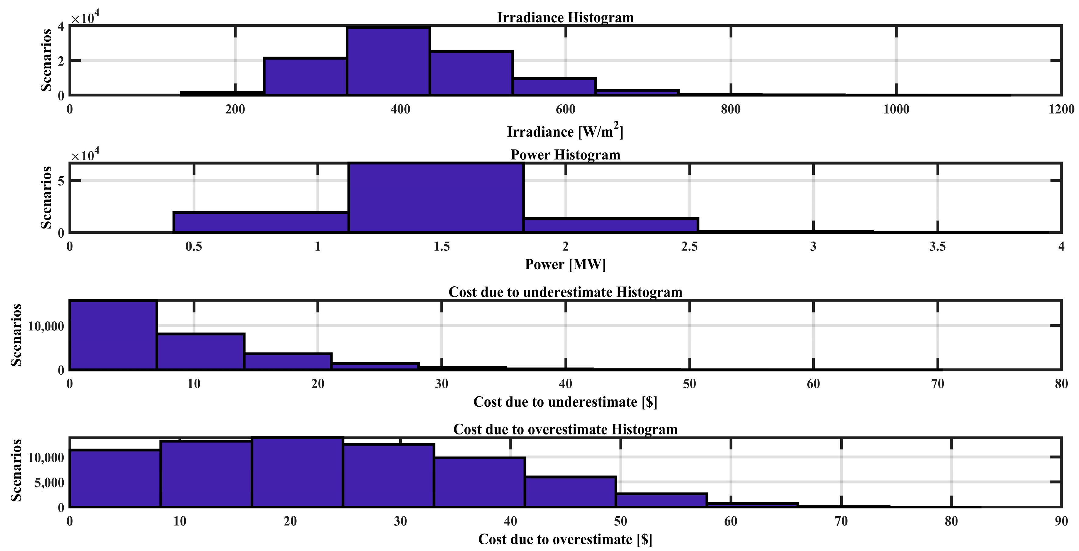
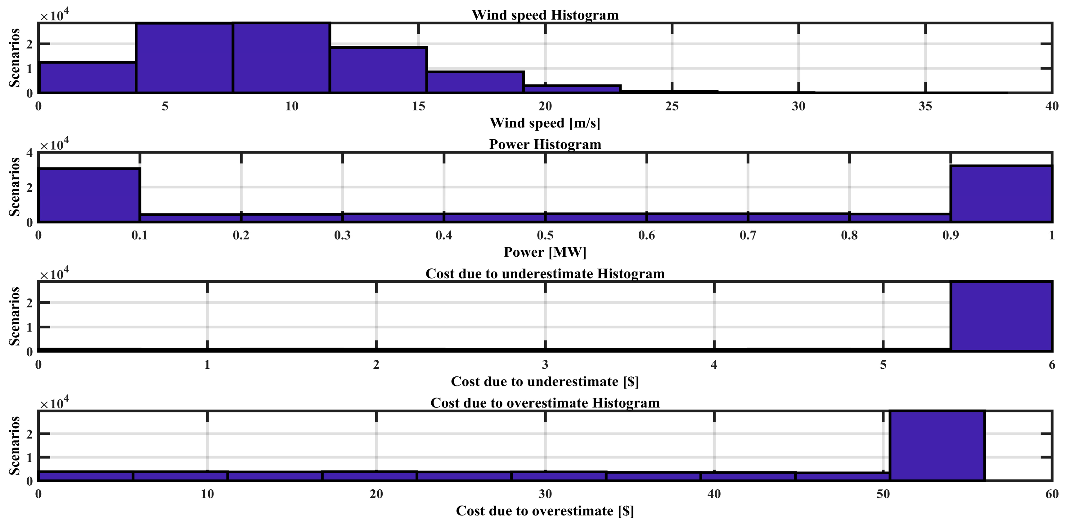
This subsection analyzes the impact of atmospheric conditions on the system’s performance, considering fixed values for capacitors (C), solar panel efficiency (PV), wind turbines (WT), and battery energy storage systems (BESSs). Figure 9 and Figure 10 highlight the correlation between solar irradiance, wind speed, and system factors such as power output, costs, and voltage characteristics. Figure 9 shows a positive linear relationship between the solar irradiance and power output from PV panels, where higher irradiance leads to increased electricity generation and reduced reliance on costlier alternative sources. Conversely, lower irradiance levels result in higher dependency on alternative power sources, raising costs. For wind turbines, Figure 10 illustrates a nonlinear relationship: power initially increases with wind flux, stabilizes within a certain range, and then rises again. This pattern underscores the importance of accurately estimating wind energy needs to minimize the costs associated with underestimating or overestimating power requirements. In both these figures, variations in underestimated and overestimated costs are shown under four scenarios with the availability of wind and sunlight (20%, 40%, 60%, and 80%). It can be observed that in the first scenario (overestimate), the power delivered to the grid is more than the demand power, so the rest will go to charging the BESS (batteries system). Similarly, in the second scenario (underestimate), the power delivered to the grid is less than the demand power, so the rest of the power will be taken from the BESS, which will be discharged.

3.5. Comparative Performance of All Four Metaheuristic Algorithms

In this section, we compared the performance of all three algorithms in terms of (1) voltage stability, (2) economic loss, (3) cost, and (5) robustness against different environmental conditions. To compare the performance, we categorized different varying conditions associated with solar irradiance and wind speed into different levels (represented in %). In the context of solar irradiance and wind speed estimation, the highest level (100%) represents the maximum expected irradiance and wind speed for the given location, and the lowest level ($\approx 0$%) represents minimum sunlight and air density. The detailed comparative study is given below.

3.5.1. Voltage Stability Factor Analysis

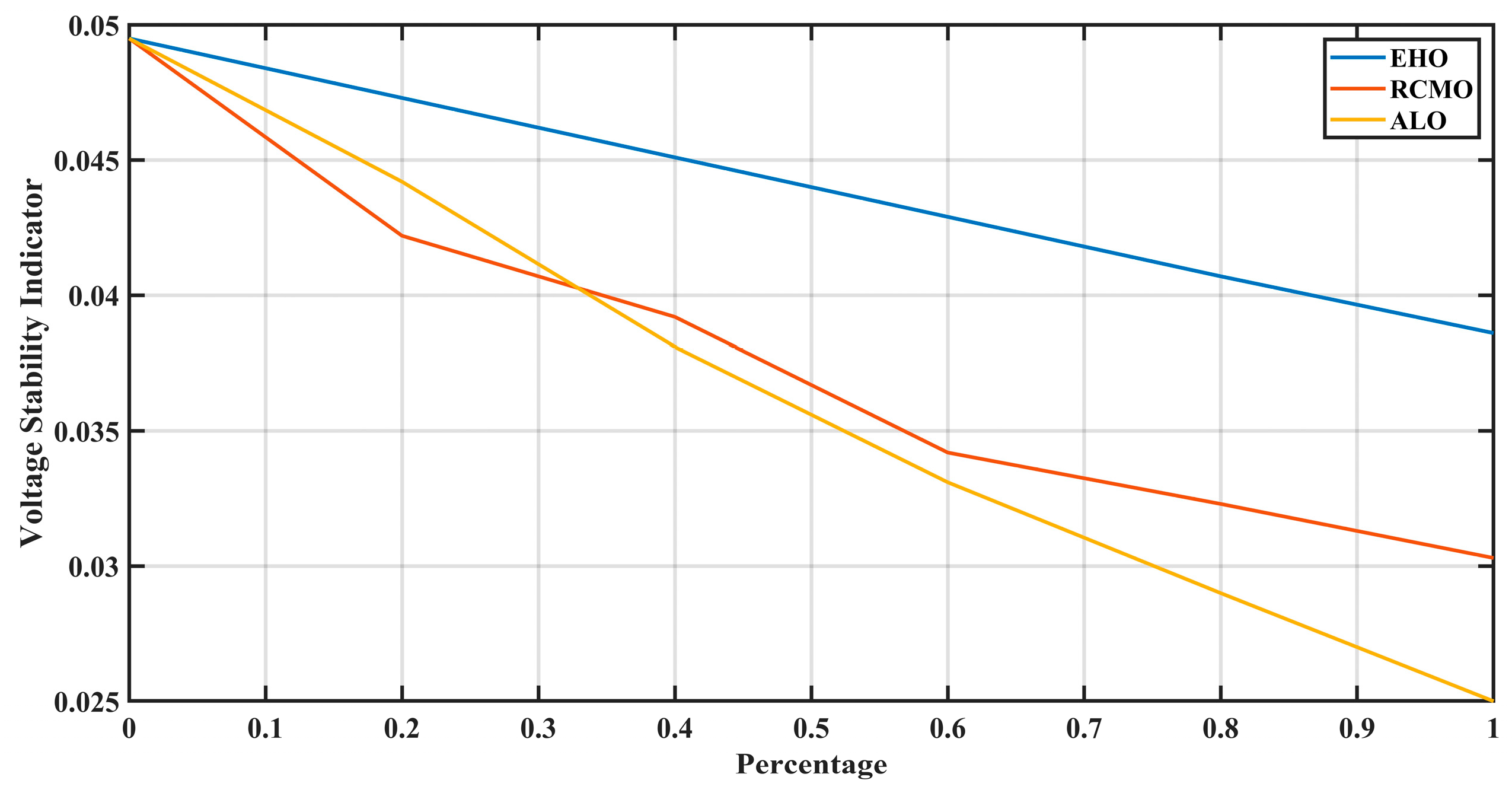
The graph shown in Figure 11 contains voltage stability graphs for three different optimization algorithms: The nature-inspired metaheuristic algorithms are Ant Lion Optimization (ALO), Elephant Herding Optimization (EHO), and Red-Colobus Optimization (RCMO). The trend observed in the graph of Ant Lion Optimization (ALO) indicates that as the percentage increases, the Voltage Stability Indicator (VSI) reduces about the percentage increase. This means that the ALO algorithm retains a constant complexion with the percentage input and voltage stability. The downward trend of the plot shows that as the percentage of distributed renewable generation and storage increases, the voltage stability decreases, proving the applicability of ALO across different voltage stability situations.

The graph for EHO shows a similar linear decreasing trend of VSI with the percentage increase. This shows a satisfactory and coherent behavior of the EHO in the improvement of voltage stability. The graph also shows the potential of the algorithm regarding the balance of distributed renewable energy resources; it is essential to minimize the voltages as the percent increases to provide reliability to the power systems. For the Red-Colobus Monkey Optimization (RCMO), there is a group of bars that displayed a linear decline of the voltage stability indicator as the percentage increased. The decline of all five indices implies that the RCMO algorithm is well suited for the coordination between voltage stability and the various levels of distributed renewable generation and storage. This probably conveys the fact that the algorithm sustains voltage stability by pointing to the continued decline of voltage fluctuations as atmosphere pressure changes. All three graphs are observed to have a linear downward trend, and this proves that both ALO, EHO, and RCMO lessen the voltage stability indicator as the added percentage of distributed renewable generation/storage increases.

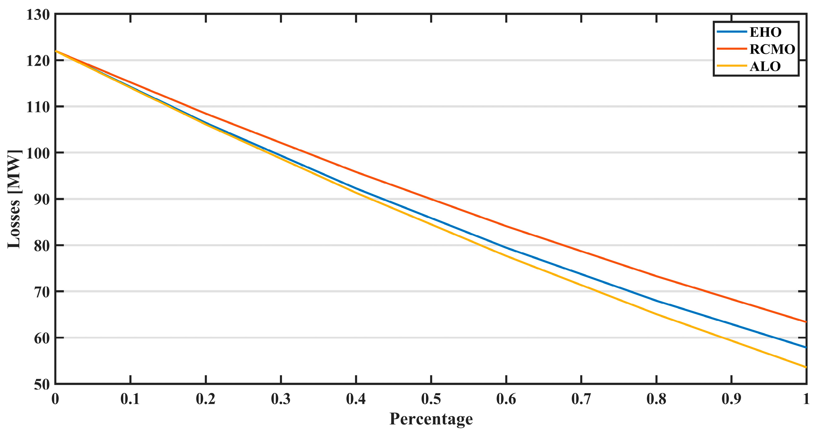
3.5.2. Loss Estimation with Varying Load of Atmospheric Conditions

Figure 12 refers to the loss estimation graph of three different optimization algorithms. The graph depicting ALO reveals the decreasing fashion of the losses as the percentage of distributed renewable generation and storage is increased. This shows that the proposed ALO algorithm helps minimize the system losses as renewable energy is integrated into the system. The curve reveals how the algorithm enhances the optimization of the system in reducing the losses, which helps enable better management of the energy and the system. Likewise, there is a considerable improvement in the losses plotted against the percentage by the EHO. As for the reduction in losses with higher levels of renewable energy integration, the EHO algorithm performs very well. They notice the tendency toward decrease, indicating that the proposition of this algorithm aids in increasing the overall efficiency of the system by decreasing losses and providing more successful energy management. The graph showing the RCMO is very similar to the graph of the Red Colobus; in this case, there is also an apparent indication of losses’ decline with the growth of percentage rates. It is evident from the analysis of the RCMO algorithm that the losses reduce progressively as more renewable generation and storage are scheduled in the system. Hence, the algorithm performed very well in this regard. This trend has shown that the RCMO is effective in fine-tuning the system for the lowest losses possible, which is important in using distributed RESsto the maximum advantage. Each of them includes a curve, which shows that the total losses progressively decrease with the rising portion of distributed renewable generation and storage. From the analysis of all the graphs, it is evident that all the algorithms result in a decrease in the amount of loss, which in turn enhances the efficiency and sustainability of the energy management system.

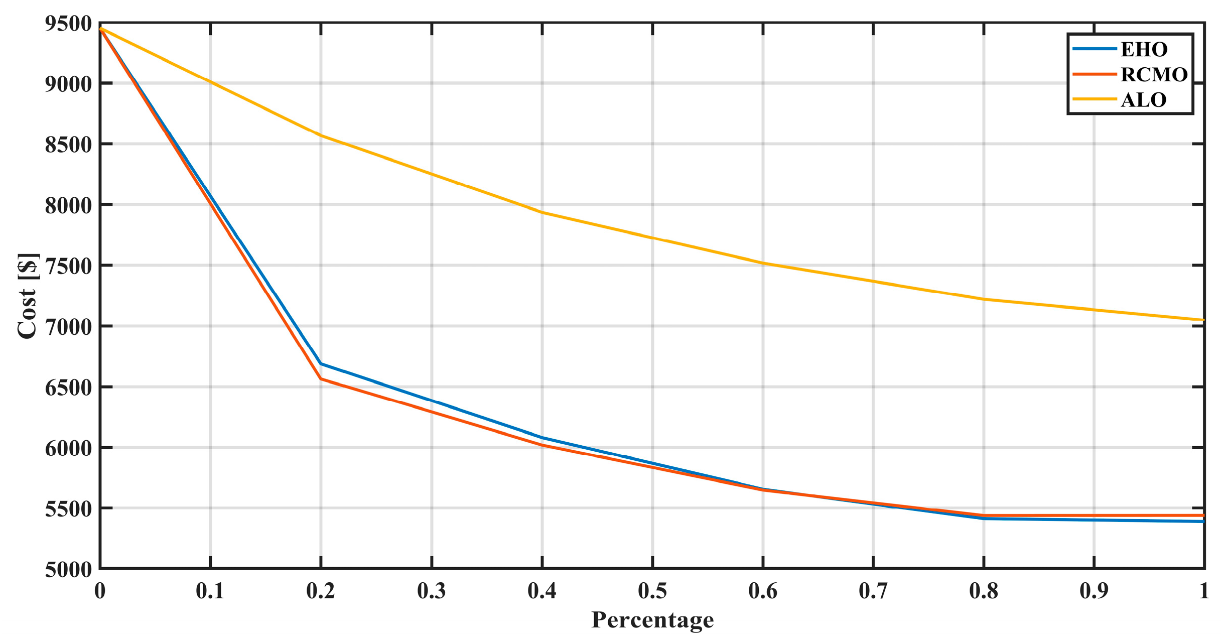
3.5.3. Cost Analysis with Varying Load of Atmospheric Conditions

Figure 13 shows the comparative result of the performance of the ALO, EHO, and RCMO algorithms in the application of minimizing the cost of distributed renewable generation and storage system placement, sizing, and coordinated power and energy control. As the percentage of renewable integration rises, the cost reduces across all the algorithms, demonstrating the effectiveness of increased integration on cost reduction. The EHO algorithm has the best performance, the largest decrease, and the lowest cost values, thus proving that the algorithm works best for this application. The RCMO algorithm stays close to EHO performance and, while being slightly more costly, is still better than ALO. However, the ALO algorithm is slow; it has a higher cost throughout the percentage range, which indicates that the algorithm is less efficient in minimizing costs than the two other approaches. This comparison reveals that all three algorithms contribute to cost reduction, while EHO and RCMO are slightly more efficient than ALO, and EHO is slightly more efficient than RCMO.

3.5.4. Robustness Against Different Environmental Conditions

This subsection covers the performance of all three metaheuristics under varying atmospheric conditions, specifically focusing on how changes in wind speed and solar irradiance affect the system’s power output and other relevant parameters. To explore the performance, we categorized the different varying conditions associated with solar irradiance and wind speed into five different levels (represented in %). In the context of solar irradiance and wind speed estimation, the highest level (100%) represents the maximum expected irradiance and wind speed for the given location, and the lowest level (20%) represents minimum sunlight and air density.

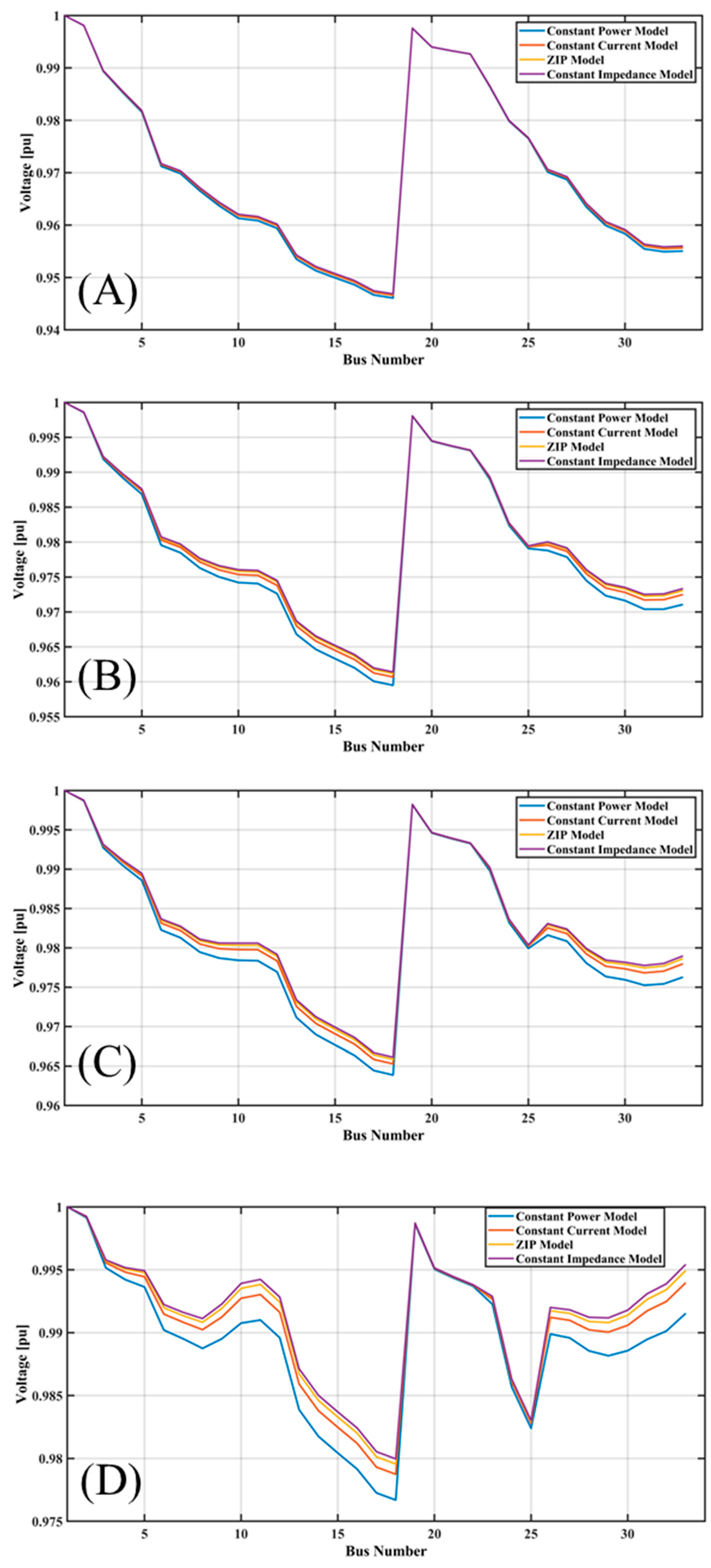
Ant Lion Optimization with Varying Levels of Atmospheric Conditions

Figure 14 provides a visual analysis of how the ALO algorithm performs in optimizing a distributed renewable energy system under varying atmospheric conditions represented as (A), (B), (C), (D), and (F). The three subplots, A, B, and C illustrate the voltage profiles of a power distribution network under four load models, namely: constant power, constant current, constant impedance, and ZIP. Figure 14A refers to the base case before optimization. Here, constant impedance loads deliver the largest voltage stability through their invariable nature whereby they make minimal voltage falls; constant power loads lead to the most significant voltage troughs resulting from the extreme current taken to sustain that constant power, and on the ZIP model that pools all loads, the general voltage distribution is midway. The largest voltage deviations occur at the terminal buses, indicating greater losses at the extremities of the network.

Figure 14B,C present the results of optimization techniques. Figure 14B indicates better voltage profiles following partial optimization, probably due to distributed generation or energy storage systems. Voltage drops are reduced across all the models, with the constant impedance model retaining the highest stability and the ZIP model balancing. In Figure 14C, optimum performance using PV-DG, BESS, and capacitor banks is achieved which has drastically improved the voltages in all buses. The constant power model showed the poorest performance at first but ended up showing marvelous improvement.

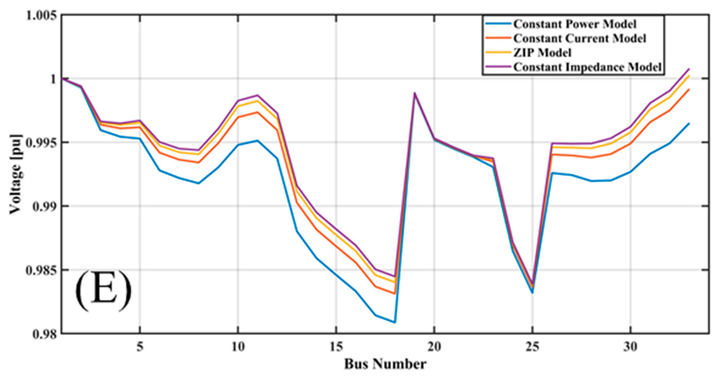
Figure 14D,E represents the voltage profiles of the distribution network using four load models at different optimization levels: constant power, constant current, constant impedance, and ZIP. In Figure 14D, intermediate optimization has increased stability in voltage with a good performance by the ZIP model, while the highest level of stability is kept by the constant impedance model. The constant power model still indicates the lowest voltages as opposed to its initial stages, but it presents improvement compared to those early levels. In Figure 14E, complete optimization, including elements such as PV-DG, BESS, and capacitor banks, results in considerable voltage stabilization across all the buses. The ZIP model remains excellent with balanced performance, while the constant power model has considerable recovery, indicating that the optimization strategy is effective in reducing voltage drops and improving network stability under different load conditions.

It can be seen from

Table 3. Performance of ALO under varying scenarios.

Scenarios (in %)	20%	40%	60%	80%	100%
Performance
Cost (×1.0 × 103) (in $/MW)	8.3662	7.4659	6.8537	6.4732	6.3620
Loss (in MW)	164.7670	145.8170	129.2684	115.0712	103.1771

that the cost value reduces as the scenario percentage rises from 20% to 100%. From the results obtained, it can be inferred that the ALO algorithm exhibits lower costs as the more favorable atmospheric conditions are available for production. This behavior can be explained by the fact that the algorithm under study provides more optimal utilization of the available renewable power related to irradiance or wind speed at levels when it was significantly higher, and thus, the need to draw on more costly power sources. The loss parameter also decreases as the scenario percentage rises, and these could, by some means, depict energy losses within the system. This means that the ALO algorithm is more useful in preventing energy loss than when other weather conditions prevail. This level of loss reduction could be attributed to the algorithm fine-tuning of the available system resources’ configuration to minimize energy loss at higher consumer resource availability.

Elephant Herding Optimization with Varying Levels of Atmospheric Conditions

Figure 15 shows the voltage graphs of a power system for different conditions of irradiance and wind percentages represented as Figure 15A–E with the help of the EHO algorithm. The voltage profiles are shown under different load-shedding scenarios across five distinct renewable energy penetration levels. The graphs represent the current total real load, current total load, and shedding concerning load shedding scenarios. This graph illustrates the performance of the voltage about the bus numbers of the system where both the irradiance and wind percent contributions are at their highest level, which is 100%. The voltage fluctuations show how the system performs when using 100% renewables; this shows stability and instabilities. The second graph shows the voltage profiles as irradiance, and wind percentages are cut at 80%. This one might be a situation with a somehow lower renewable energy feed-in, indicating how the voltage profile is steady or unstable in these conditions against the 100% situation. In the third level (60%), reducing the input of renewable energy continues to alter the voltage profile while showing more information on the performance of the system under relatively moderate levels of renewable energy. The second last case (40%) shows the voltage characteristics of the respective system at 40% irradiance and wind percentage. The fifth graph, on the other hand, shows the voltage of the respective bus numbers in the power system as the irradiance and wind percentages are set at 20%. This position analyzes a situation where the rate at which the grid consumes renewable energy is significantly low and mimics a scenario where sunlight and wind energy are scarce. This no-go zone will rarely happen, like an overcast evening when the wind is scarce.

The quantitative simulation results given in

Table 4. Performance of EHO under varying scenarios.

Scenarios (in %)	20%	40%	60%	80%	100%
Performance
Cost (×1.0 × 103) (in $/MW)	5.7005	4.2758	3.4912	3.1771	3.3557
Loss (in MW)	110.1147	82.5893	62.5910	49.7225	43.6254
Voltage Stability	0.0313	0.0258	0.0204	0.0152	0.0100

highlight the behavior of a power system in terms of capability under different levels of irradiance and wind percentage, namely 20%, 40%, 60%, 80%, and 100%. It can be observed that while achieving 20% renewable energy penetration, the system experiences its highest performance cost of 5.7005, which means three main operational expenses because of low contribution from renewable sources. Consequently, the voltage stability is the lowest at 0.0313, implying that the voltages of the network cannot be stabilized while accepting very little renewable power. When the penetration level of RESsis is 40%, the performance cost reduces to 4.2758. Although the role of renewables in power generation is increasing, efficiency is also rising. The system’s losses were reduced to 82.5893, demonstrating better energy utilization. The level of voltage stability increased to 0.0258, which has a better flatness in voltage regulation under these conditions. This specific cost dropped down to 3.4912 when the renewable energy penetrated up to 60%, resulting from higher operating efficiency during the year. The losses reported were comparatively less at 62.5910, which also confirmed successive enhancements of energy effectiveness. The voltage stability improved to 0.0204, which showed improved voltage stability as the renewable energy contributions increased. Thus, with 80% renewable integration, the performance cost was reduced to 3.1771, which is one of the lowest operation expenses out of these scenarios. The losses decreased to 49.7225, signifying substantial gains in the energy efficiency. The voltage stability significantly improved to 0.0152, indicating strong stability with high renewable input. While the renewable resources were at 100%, the performance cost was recorded to be slightly higher at 3.3557 compared to the 80% scenario, which could be explained by the system’s transitions to completely renewable energy. However, this scenario experienced the lowest losses at 43.6254, indicating optimal energy efficiency. The voltage stability was highest at 0.0100, demonstrating excellent stability with full renewable energy input.

Red Colobus Monkey Optimization with Varying Levels of Atmospheric Conditions

The plots shown in Figure 16 depict the voltage characteristic of a power system in case of various percentages of the irradiance and wind speed represented as (A), (B), (C), (D), and (E) using the Red Colobus Monkey Optimization (RCMO) technique. In this case, when irradiance was at 100%, and wind speed was also at 100%, the voltage profile with bus numbers changed drastically because of highly distributed generation. The constant power model had even sharper ups and downs, which suggests that there is a possibility of poor stability. The model, including constant power, impedance, and current elements, was the ZIP model, and its response appeared to be more balanced, meaning that it could better accommodate high penetration of renewables.

Analyzing the results, 80% of irradiance and wind speed have resulted in a relatively stable voltage level as compared to the 100% voltage level symmetric across the bus numbers. The constant power and the constant current models also have considerable voltage fluctuations, though the changes are appreciable to a lesser extent. The constant impedance model and ZIP model depict a far more stable voltage profile, which suggests that the system is much better equipped to deal with slightly less input from the renewables. This particular case illustrates the enhancement of system stability when using a slightly reduced amount of renewable energy. Interestingly, as the renewable penetration increases, the voltage profile becomes better throughout all load models for 60% renewable penetration. The compliance with the constant power model is nevertheless not perfect. It appears slightly more oscillating in these cases, but the variations are much less emphasized than in the outlined higher renewable input constellations. Thus, the constant impedance and ZIP models show rather smooth voltage curves, and the system stability increases as the share of RESs decreases. This scenario indicates that the power system will be capable of managing supply voltage with a medium level of renewable power penetration into the system.

From

Table 5. Performance of RCMO under varying scenarios.

Scenarios (in %)	20%	40%	60%	80%	100%
Performance
Cost (×1.0 × 103) (in $/MW)	6.2941	5.1059	4.3979	4.0032	3.9859
Loss (in MW)	120.3322	99.1826	81.4334	66.9539	55.6223
Voltage Stability	0.0387	0.0349	0.0311	0.0274	0.0237

, we can see the performance measures of the power system optimized with the RCMO technique under different practicing levels of irradiance and wind speed percentages. Thus, the cost was observed to reduce for each increase in the rate of renewable energy, meaning a higher efficiency in operation with a high percentage of renewable energy. This is noted to be slightly higher than the previous estimates when the renewable share was at 20%, and the total cost was estimated to be 6.2941. When the share of renewable generation sources was raised to 40%, 60%, 80%, and 100%, the level of costs turned down to 5.1059, 4.3979, 4.0032, and 3.9859, respectively. This phenomenon implies that relying on a greater level of renewables leads to decreased functional expenses.

At 20% renewable penetration, the costs were highest at 120.3322 $/MWh for the system that experienced the highest loss. There was a corresponding increase in the conventional generation, which impacted efficiency, hence the high figure. As the renewable energy percentage increased, the losses decrease significantly: 99.1826 at 40%, 81.4334 at 60%, 66.9539 at 80%, and 55.6223 at 100%, respectively. This trend depicts that with the increasing contribution of renewable energy, energy utilization was better, and power losses were smaller. Voltage stability defines the capability of the network to maintain suitable voltage levels in the course of delivery. Lower values represent higher stability in which the voltage does not go significantly above or below its desired range. As for the 20% penetration of renewable sources, the voltage stability measure was 0.0387, which is the highest among the scenarios, inferring that the system encounters the greatest difficulty in stabilizing the voltages. In this scenario, voltage stability increases, which is evident from the reduction in values to 0.0349 as the share of renewable sources gets higher at 40%, 0.0311 at 60%, 0.0274 at 80%, and 0.0237 at 100%. This leads to the conclusion that higher offices of renewable energy improve the voltage strength of the system.

3.6. Comparative Performance Study

The results given in

Table 6. Statistical results computed from metaheuristic algorithms after the optimization.

	Anti-Lion Optimization	Elephant Herding Optimization	Red Colobus Monkey Optimization
Voltage Stability	0.0024115	0.0031346	0.0052053
Real Power Losses before	202.6771	202.6771	202.6771
Real Power Losses after	7.5092	22.6775	20.7564
Capacitor Values (Mvar)	1.9197	2.9421	1.9894
Solar Panel Values (MVA)	1.0278	1.439	1.0159
Wind Turbine Vales (MVA)	1.0936	0.8568	1.7529
Battery Value (MVA)	0.3032	1	0.299

provide a comparative analysis of all three metaheuristic optimization algorithms in the problem of optimizing distributed renewable generation and storage systems. In terms of voltage stability, the Ant Lion Optimization algorithm estimates the best performance with an index of 0.0024115, indicating superior stability. This is followed by Elephant Herding Optimization, recording a stability index of 0.0031346, and Red Colobus Monkey Optimization, having a stability index of 0.0052053. Lower values represent better voltage stability. The second performance metric is real power loss, determining the total power losses in the electrical system before applying the power optimization method. These losses occur because there is always some resistance in the transmission lines, transformers, and other equipment that leads to the wastage of energy in the form of heat. The real power losses after optimization refer to the total power losses once an optimization algorithm, such as ALO, EHO, and RCMO, has been applied. Such optimization aims to minimize these losses through better deployment and scale of distributed generation systems like wind, solar, and battery energy storage. Regarding real power losses, all algorithms initially start with losses of 202.6771 MVA. After optimization, Ant Lion Optimization significantly reduced these losses to 7.5092 MVA, the lowest of the three. In comparison, the Red Colobus Monkey Optimization achieves a reduction of 20.7564 MVA, while the Elephant Herding Optimization results in losses of 22.6775 MVA.

The optimized capacitor values show some variability, with the Elephant Herding Optimization requiring the highest value at 2.9421 Mvar. Red Colobus Monkey Optimization and Ant Lion Optimization need 1.9894 Mvar and 1.9197 Mvar, respectively. For solar panel capacities, Elephant Herding Optimization requires 1.439 MVA, Ant Lion Optimization requires 1.0278 MVA, and Red Colobus Monkey Optimization requires 1.0159 MVA. Wind turbine power or apparent power varies significantly, with the Red Colobus Monkey Optimization suggesting the highest capacity at 1.7529 MVA. Ant Lion Optimization proposes a capacity of 1.0936 MVA while Elephant Herding Optimization proposes a capacity of 0.8568 MVA. It reflects the sum of active power MW, which is the real usable power, and the reactive power MVAR, which supplies the voltage levels for the transfer of real power. Apparent power is also expressed in mega volt-amperes (MVA) and stands for total power provided in a circuit, which includes active and reactive. In terms of battery capacities, Elephant Herding Optimization requires 1 MVA, Ant Lion Optimization requires 0.3032 MVA, and Red Colobus Monkey Optimization requires 0.299 MVA. Overall, Ant Lion Optimization demonstrates the most effective performance in minimizing real power losses and achieving the best voltage stability. Elephant Herding Optimization and Red Colobus Monkey Optimization also show substantial improvements in system parameters, although they do not match the performance of Ant Lion Optimization.

The proposed optimization framework has more advantages over the conventional approach to grid management through enhanced adaptability to prevailing conditions, improved voltage stability, and optimal siting and sizing of distributed resources. The integration of four different load models, namely constant impedance, current, power, and ZIP, has tried to capture a wider spectrum of variability associated with loads in real-world application scenarios. Traditional approaches often assume constant or foreseeable load conditions and are prone to losing track when such changes occur suddenly. In classical grid management, small perturbations in the voltage level or renewable energy power production are largely not responded to, and hence, potential instability may arise. Metaheuristics are proposed along with direct impacts on the optimization of the voltage stability index and minimization of real power losses, namely, Elephant Herding Optimization, Modified Ant Lion Optimization, and Red Colobus Monkey Optimization. For instance, Modified Ant Lion Optimization achieves a voltage stability index at 0.0024115 while most conventional methods cannot, which represents renewables generation variabilities, thereby ensuring a robust grid that can then maintain steady states by staying resilient to the intermittency of renewable resources. This will place renewable and storage resources where they can best contribute to the grid and match their capacities to actual demand and grid conditions, thus enhancing both reliability and energy efficiency.

3.7. Computational Complexity

To evaluate the computation complexity of the proposed framework, we divided our approach into two key steps: (1) the execution of metaheuristic algorithms and (2) fitness function computation. The computational complexity for all three algorithms is linear and represented as $O\left(P\ast I\right)$, where $P$ indicates population size, and $I$ refers to the number of iterations used in the study. Further, the fitness function defined in Equation (9) is linear with $O\left(n\right)$; therefore, the overall complexity of the $O\left(P\ast I\ast F\right)$ is where F is the cost function evaluation time (which includes power flow calculations). Since we are executing three different algorithms, the overall computational complexity can be approximated using Equation (50).

$$O \left(P_{EHO}\ast I_{EHO}+P_{ALO}\ast I_{ALO}+P_{RCMO}\ast I_{RCMO}\right)\ast F$$

(50)

This is the total time complexity, depending on the number of iterations and the complexity of each power flow calculation.

3.8. Limitations of the Proposed Study

Although promising results have been reported, the proposed optimization framework is not without limitations. Notably, there is considerable computational complexity related to its implementation using three advanced metaheuristic algorithms: Red Colobus Monkey Optimization, Elephant Herding Optimization, and Modified Ant Lion Optimization. Those algorithms require large amounts of computation and time, significantly in the case of very large power distribution systems where search spaces are high dimensional. This may render the solution not practical for real-time applications or even for larger networks. The dependency on proper data inputs such as wind speed, solar irradiance, and load demand patterns is another limitation. Since the performance of the framework is highly sensitive to the inputs, inaccuracies or fluctuations in data may lead to less-than-optimal results. Thus, the method is less effective in scenarios involving high uncertainty or unreliable availability of data, which often characterizes renewable energy systems.

4. Conclusions and Future Scope

In the proposed study, we developed a mathematical model for the accurate location, scale, and coordinated power, and energy of distributed generations (PV-DG) and storage systems (BESSs). In our model, we employed four different load models and components, such as wind turbines, PV, capacitor banks, and BESSs, to capture the dynamic load demand. Our approach utilizes the functionalities of three metaheuristics: (1) Ant Lion Optimization, (2) Elephant Herding Optimization, and (3) Red Colobus Monkey Optimization, for determining optimal solutions (high voltage stability, least power loss, and minimum implementation cost). To analyze the performance of all three algorithms, we categorized the different conditions associated with solar irradiance and wind speed into five levels (represented in %). It has been shown that the Ant Lion Optimization (ALO) algorithm is the most effective approach for optimizing distributed renewable energy systems under different climatic conditions. According to the analysis, the algorithm works best in ideal circumstances, namely when the percentages of wind and irradiance are 60% or greater. The Modified Ant Lion Optimization achieved a best voltage stability index of 0.0024115 and power losses of 7.5092 MVA. This scope was the least among all three algorithms. The ALO algorithm shows its flexibility as atmospheric conditions vary, efficiently lowering expenses and energy losses even as these parameters shift.

The results of this study can be applied to real-time energy management systems, specifically for optimizing distributed renewable energy systems, including PV-DGs, wind turbines, and energy storage systems (BESSs) in smart grids and microgrids. This way, the model, as proposed, can take into consideration real-time data coming from weather sensors and the load grid, thus enhancing stability, and reducing power losses, and operational costs. It can also be used on energy trading platforms for dynamic market participation, adjusting the energy distribution based on present conditions. Future extensions include incorporating IoT sensors, hybrid optimization algorithms, and scenario-based multi-objective optimization for more effective decision-making. Additionally, the model could be scaled for large regional or national grids and adapted to predict long-term climate impacts, thus being a crucial tool for immediate optimization and long-term energy planning.