Collaborative Scheduling Optimization of Container Port Berths and Cranes under Low-Carbon Environment

Abstract

Motivated by the need for a green and low-carbon economy, we explore the co-scheduling optimization of berths and cranes. Our aim is to balance the carbon tax and operating costs of ports under uncertain conditions, proposing an innovative nonlinear mixed-integer programming formulation. To address this optimization challenge, we have developed an enhanced version of the adaptive spiral flying dung beetle algorithm (ASFDBO). In order to evaluate the performance of the ASFDBO algorithm, we performed a benchmark function test and a convergence analysis with other recognized metaheuristics. In addition, we verified the practical applicability of the ASFDBO algorithm in different test scenarios. Through numerical experiments, we analyze the feasibility and effectiveness of the algorithm’s scheduling solutions and improvement strategies. Results indicate that our collaborative scheduling optimization, which considers both carbon and production costs, achieves feasible solutions and reduces carbon expenses. Finally, we investigate the impact of different carbon tax rates on the joint scheduling optimization of berths and quay cranes, and the results show that a reasonable carbon tax policy can effectively reduce the carbon emissions of ports.

1. Introduction

Serving as a crucial connection between maritime and inland transport, the container terminal plays a vital role in collecting and buffering cargo and facilitating the conversion of transport modes. In the increasingly competitive environment of container terminals, answering the question of how to improve the efficiency of resource utilization and service levels has become a key issue for terminal operators. Among the numerous equipment resources of a terminal, berth resources are the most important strategic resources. Usually, terminals will achieve efficient use of berth resources by formulating reasonable berth scheduling plans and optimizing the berth scheduling process. This scheduling considers the vessel arrival plan, the number of available berths, crane availability, and resource constraints such as crane frontage. The primary uncertainties revolve around vessel arrival times and the duration of vessel loading and unloading activities. Variations in loading and unloading times are mainly attributed to crane failures and efficiency fluctuations. The dynamic nature of vessels and cranes poses a challenge, rendering the scheduling plan unfeasible due to constant state changes.

A schematic diagram of the berth quay crane operation process in a container terminal is shown in Figure 1. Upon arrival of the vessel, berthing and mooring operations are required to ensure that the vessel is firmly berthed at the berth. A quay crane is a piece of equipment used to lift containers and is responsible for unloading and loading the cargo from the vessel. The efficiency of this stage directly influences the effectiveness of the overall port operation. Once the loading and unloading is complete, the containers are transferred to storage areas within the port, where they are handled by various means of transport. Throughout the operation, the port management system records critical operational data, such as unloading and loading times, for subsequent analysis and optimization. In addition, relevant information is passed on to other relevant departments or systems to ensure the coordinated operation of the entire supply chain. Vessels leave the berth after completion of their loading and unloading tasks. The entire berth quay crane operation flowchart is a complex and coordinated system that requires efficient scheduling and collaborative work as a means of maximizing the utilization of quay cranes and other equipment, ensuring that they operate efficiently most of the time, and maximizing the operational efficiency of the port.

As an essential part of the transportation sector, ports are sites of high fossil energy consumption and greenhouse gas emissions, the primary sources of which are associated with vessels berthing at ports. As the total amount of cargo transportation continues to increase, the pressure to reduce emissions at ports will be further aggravated. The question of how to realize energy saving, emission reduction, and the green transformation of ports has become the focus of social attention [1]. Maritime transportation contributes approximately three per cent of global carbon dioxide emissions annually. The Port of Rotterdam has taken several initiatives to work towards a more sustainable urban development through the Rotterdam Climate Agreement and is committed to reducing emissions by fifty per cent. In addition, the World Ports Climate Action Program (WPCAP) focuses on improving energy efficiency, developing green onshore power sources, promoting alternative energy sources, and utilizing policy instruments to reduce maritime emissions. The recent inclusion of shipping in the European Union’s Emissions Trading System (ETS), which requires shipping companies to purchase a percentage of carbon allowances for voyages within and to and from the European Union, marks the formal entry of the shipping industry into the era of sustainability.

Given that the problems covered in this paper are NP-hard problems, i.e., non-deterministic polynomial problems whose solution time complexity usually grows exponentially, it is only possible to verify the correctness rather than the optimality of a solution in polynomial time. An efficient algorithm for solving such problems has not been found. Compared with other studies in this field, which are based only on the assumption that cranes will not fail, the research in this paper also covers the crane maintenance planning problem. It considers several constraints, such as uncertainties in ship arrival time, crane operating efficiency, and mutual interference between cranes. As a result, the proposed nonlinear integer model is more complex, and it is difficult for the exact algorithm to find the optimal solution in polynomial time as the problem size increases. While commercial solvers, such as CPLEX and Gurobi, are usually used for linear programming models, they cannot solve the nonlinear integer programming model developed in this paper. This kind of problem can only be solved by some heuristic algorithms or meta-heuristic algorithms to quickly obtain a satisfactory solution. This paper chooses a novel dung beetle optimization algorithm (DBO) as a solution tool. The main reason for choosing this algorithm is that it exhibits faster convergence and a better ability to solve complex problems in terms of optimization performance than other algorithms, such as WOA and GWO. At the same time, the algorithm is relatively simple in principle, easy to understand and implement, and usually requires fewer parameters to be adjusted, making it easier to apply to different problems. However, it also has some drawbacks, which include the uneven distribution of the initial population, the imbalance between global exploration and local exploitation capabilities, the ease with which it falls into local optimal solutions, and its weak global search capabilities. Therefore, the DBO algorithm needs to be improved. First, Bernoulli’s chaotic mapping can improve the distribution quality of the initial population in the search space to enhance its global search ability. Second, adaptive weighting and Lévy flight mechanism are introduced to help individuals freely explore the global and local optimization within the region given by the algorithm in order to expand the search space and to gradually converge to the same optimal solution or objective function value, thus enhancing global optimization ability. The adaptive weighting factor can enhance the global exploration ability at the beginning of the algorithm iteration while improving the local exploitation ability later in the iteration. Such a design can reduce the risk of falling into a local optimal solution and enhance the local search ability, effectively improving the operation efficiency of the algorithm. In addition, using the variable spiral search strategy to balance the global and local search capabilities while performing the Gauss–Cauchy hybrid variant perturbation operation can increase the diversity of the dung beetle population, enabling the algorithm to jump out of a local optimal solution and continue to explore in other regions of the solution space until the global optimal solution is found.

Therefore, this paper aims to study a joint berth and quay crane scheduling optimization problem that takes into account both carbon and operational costs, also taking into account the uncertain vessel arrival time, the imprecise operational efficiency of the quay cranes, the interference between quay crane operations, and the maintenance schedule of quay cranes. On this basis, we constructed a mixed integer planning model for minimizing the comprehensive cost of vessels in port and designed an adaptive spiral flight dung beetle algorithm to solve it. Eventually, we obtained a joint scheduling scheme that satisfies the port’s low-carbon benefits and interests and realizes the port’s scientific management and energy saving and emission reduction goals.

2. Literature Review

The competitiveness of a port is significantly influenced by the effective management of the berth allocation problem (BAP) and the quay crane scheduling problem (QCSP), which are fundamental components of container terminal production operations. Hence, numerous domestic and international scholars have sequentially investigated scheduling issues concerning independent and collaborative scenarios for container terminal berths and quay cranes, considering both deterministic and uncertain environments. Bierwirth and Meisel [2,3] put the spotlight on the container terminal frontier operations, categorizing them according to different attributes, such as spatial layout, vessel arrival time, and operation time.

Jiao et al. [4] introduced the tidal influence factor, on the basis of which the main consideration is the impact of tides on the transportation capacity of the connecting terminal and the transportation capacity of the inlet channel connecting the wharf and the anchorage. Soroush and Reza et al. [5] focused mainly on tidal influences, draft depth limitations, and safe distances in and out of the harbor. Bierwirth and Meisel [6] considered the factor of mutual interference between quay cranes and designed a heuristic algorithm based on the branch and bound (B&B) algorithm to obtain the final scheduling plan after constructing an optimization model. Hsu and Wang [7] proposed a two-stage approach to generate the berthing sequence of the vessels, firstly by the multi-particle swarm optimization (MPSO) algorithm and then by designing an event-based heuristic algorithm to determine the final berthing plan and quay crane allocation plan. Agra and Oliveira [8] investigated the scheduling problem involving both berth and cranes in a port with varying sizes of quay cranes. They also formulated a mathematical optimization model using the relative position formulation (RPF), which did not involve significant M constraints. Additionally, they introduced the rolling horizon heuristic (RHH) algorithm to tackle large-scale instances. Wang X et al. [9] designed a class of double-chain molecular structure-based chemical reaction algorithms (CRAs) to solve the quay crane scheduling problem.

Park et al. [10] incorporated buffer time to manage the uncertainty of vessel arrivals. This approach involved modeling the berth allocation problem as a two-stage stochastic optimization model, with a proposed solution method utilizing a particle swarm optimization algorithm. Han et al. [11] and Liang and Wu [12] explored the joint berth and crane scheduling problem in the presence of uncertainties related to vessel arrival time and quay crane operation time. The distinction lies in Han et al.’s focus on discrete berths, employing a genetic algorithm based on simulation to address the issue. On the other hand, Liang and Wu targeted continuous berths, incorporating buffer time to account for uncertainties. They introduced an enhanced genetic algorithm, combining an adaptive genetic algorithm and heuristic berthing, to solve the problem. Zhen et al. [13] and Xiang and Liu [14] have investigated the problem of the joint allocation of berths and cranes in an uncertain vessel arrival time and with loading and unloading operations. Among these, Zhen et al. developed a two-stage stochastic optimization model for a low-carbon environment and designed a solution algorithm using a column generation technique. Xiang and Liu applied the K-means clustering algorithm to categorize and assign weights to an uncertain set. They used this approach to construct a robust optimization model, aiming to minimize both the positional deviation and departure delay costs. Krimi et al. [15] investigated the multi-terminal BAP and QCAP, employing a heuristic algorithm centered around the rolling strategy. Their study specifically targeted bulk ports, limiting the applicability of their findings to container terminals. On a related note, Bouzekri et al. [16] studied a tidal harbor with multiple jetties by combining BAP and time-varying QCAP. Considering the tidal variations and the maximum outreach of the cranes, the researchers devised an integer programming model to solve these complex problems. Similarly, Lujan et al. [17] developed a fuzzy optimization model to solve the BACAP problem by expressing uncertainties through triangular fuzzy numbers. The model can accommodate the uncertainty associated with these time-dependent variables. Rodrigues et al. [18] developed a two-stage robust optimization model to deal with ship arrival time uncertainty, decomposed the algorithmic problem into a master problem and a sub-partition problem, and solved it using a decomposition algorithm based on a hot-starting technique. Mohammadi and Forghani [19] investigated the continuous berth problem under arrival time uncertainty, using a sequence pair representation to solve the problem using a space that is projected into two permutations and a scenario-based approach to capture the uncertainty.

With the implementation of low-carbon-related policies, the question of how to reduce carbon emissions from ports has attracted much attention from researchers in some recent studies. Venturini et al. [20] took the vessel’s route speed into account in their model, and the vessel’s sailing speed produced different carbon emissions. They finally proved the effect of speed on carbon emissions and fuel consumption through arithmetic examples. Wang et al. [21] investigated a co-optimization model for berths and quay cranes in a deterministic environment, which was solved by the branch bonding method, and the operation of operations under different carbon emission policies was considered in their study. Equipment allocation problems and numerical experiments were conducted to compare different policies. Arijit and Saurabh et al. [22] considered fuel cost, berthing waiting time, and operation time issues and the advantages of the mixed integer programming model in fuel saving and port service cost reduction were verified. Wang et al. [23] constructed a multi-objective joint scheduling model for vessels with minimized delay time and minimized total cost of crane operation based on port carbon tax policy considerations. A heuristic algorithm with an integrated balance box was developed to solve the problem. Liu and Ge [24] explored AGV-equipped container ports, applying queuing theory to analyze internal queuing behavior, and developed convex optimization models for quay crane scheduling and to minimize CO₂ emissions during container loading and unloading.

Several scholars have focused on applying innovative technologies in port operations to improve efficiency and effectiveness. Abou Kasm and Diabat [25] have analyzed the scheduling problem of an innovative terminal with a short bridge capable of handling four containers in two adjacent harbors. Tan et al. [26] investigated the automated quay crane scheduling problem (AQCSP) within an automated container terminal. Jonker et al. [27] conducted a study of intra-terminal operation. The joint scheduling of resources such as quay cranes, AGVs, and yard bridges was modeled based on the hybrid flow shop (HFP) model, allowing bidirectional flow and job pairing.

By combing and summarizing the above literature, one can see that most of the existing research results take the economic benefits of ports as their starting point. Few studies have balanced the economic and ecological benefits of port operations simultaneously. In scheduling problems that consider energy consumption or carbon emission factors, most aim to minimize energy consumption or carbon emissions, but only some studies have explored the cost of a carbon tax. Meanwhile, the algorithm for solving the model should be adjusted and improved according to the model. Therefore, this paper proposes a cooperative scheduling optimization model for berths and cranes, taking into account port operation costs and carbon tax costs. Furthermore, this paper seeks to design an ASFDBO algorithm for solving the model and to analyze the influence of carbon tax costs on the model.

3. Materials and Methods

In Section 3.1 and Section 3.2, we propose a new mathematical model for the joint scheduling of berths and quay cranes in uncertain environments, taking into account the maintenance of quay cranes. In Section 3.3, an adaptive spiral flight dung beetle algorithm is designed and the effectiveness of the ASFDBO algorithm is verified. In Section 3.4, the algorithmic flow and problem-solving steps are described in detail.

3.1. Model Assumptions and Notations

• The berths are continuous, and vessels can moor at will within the limits of the quay bridge that meets their requirements.
• The length of the quay’s shoreline is known, and the water depth along the frontage meets the draught requirements of all vessels.
• When multiple quay cranes serve the same object, the efficiency of the work is reduced due to mutual interference. In addition, the relative positions of the cranes remain constant.
• The actual arrival time of the vessel and the operational efficiency of the cranes at the terminal are represented through a table of random variables following a normal distribution.
• The maintenance schedules of the quay cranes are known, the cranes in maintenance activities are not available to serve the vessels, and the corresponding berths are not available for berthing of the vessels.

The constant in the model are as

Table 1. Constant definition.

Symbol	Definition
$V$	Aggregation of vessels to be dispatched, $V=\left\{1,2,\cdots {,N}_V\right\}$
$Q$	Aggregation of quay cranes, $Q=\left\{1,2,\cdots {,N}_Q\right\}$
$Q_R$	Set of quay cranes collection within the repair plan
$L$	Length of quay
$\mu$	Expected operational efficiency of cranes
$\gamma$	Interference factor between cranes,$n$ quay cranes generate $n^{\gamma }$ effective operation periods per unit time
$b_i^e$	Desired berthing position of the vessel $i$,$i\in V$
$l_i$	Length of vessel including safety distances, $i\in V$
$W_i^U$	Cargo loads to be exported by vessel $i$, $i\in V$
$W_i^D$	Cargo loads to be imported by vessel $i$, $i\in V$
$y_i^a$	Scheduled arrival time of vessel $i$,$i\in V$
${ED}_i$	Scheduled departure time of vessel $i$,$i\in V$
$Q_i^{min}$	The minimum allocation of quay cranes to vessel $i$, $i\in V$
$Q_i^{max}$	The maximum allocation of quay cranes to vessel $i$,$i\in V$
$c_b$	Penalty cost per unit distance the vessel deviates from its intended position
$c_w$	Terminal crane unit time operating costs
$c_d$	Penalty cost per unit of time for vessel $i$ to leave overtime
$c_p$	Crane maintenance costs per unit of time
$c_{CT}$	Carbon emissions per unit of time from vessels
$c_i$	Carbon emission factor for vessels
$\rho$	Carbon tax rate
$M$	A large enough positive number
$\beta$	Berth deviation factor
$p_q$	The time for the quay crane to carry out maintenance activities
$r_q^{min}$	The earliest start of maintenance for the quay crane $q$
$r_q^{max}$	The latest start of maintenance for the quay crane $q$

, and the decision variables and Auxiliary decision variables are as

Table 2. Variable definition.

Symbol	Definition
$b_i$	Actual berthing position of vessel $i$, $i\in V$
${\vartheta }_{itq}$	If the quay crane $q$ serves the vessel $i$, ${\vartheta }_{itq}=1$; otherwise, ${\vartheta }_{itq}=$0, $i\in V$, $q\in Q$, $t\in T$
$Q_{it}$	The number of quay cranes served to vessel $i$ at time $t$, $i\in V$, $t\in T$
${\omega }_{itq}$	If the quay crane $q$ moves the vessel $i$, ${\vartheta }_{itq}=1$; otherwise, ${\vartheta }_{itq}=$0, $i\in V$, $q\in Q$, $t\in T$
$r_q$	Quay crane $q$ start maintenance time
${\theta }_i$	Relaxation variables for the arrival time of vessel $i$, $i\in V$
${∆}_i^v$	Slack variables for the efficiency of quay crane work in the service of passing vessel $i$, $i\in V$
$y_i^b$	The berthing time of the vessel $i$, $i\in V$
$y_i^d$	Actual departure time of vessel $i$, $i\in V$
${\delta }_{ij}$	If the vessel $j$ berths to the right of vessel $i$, ${\delta }_{ij}=1$; otherwise, ${\delta }_{ij}=$0, $i$, $j\in V$, $i\ne j$
${\epsilon }_{ij}$	If the vessel $j$ berths after the departure of vessel $i$, ${\epsilon }_{ij}=1$; otherwise, ${\epsilon }_{ij}$=0, $i$, $j\in V$, $i\ne j$
${\tau }_{it}$	If the vessel $i$ is operating in port at time $t$
${\alpha }_{iq}$	If the vessel $i$ is located in front of the quay crane $q$ requiring maintenance, $i\in V$, $q\in Q_R$
${\phi }_{tq}$	If the quay crane$q$ be repaired at time $t$, ${\phi }_{tq}=1$; otherwise, ${\phi }_{tq}=$0, $t\in T$, $q\in Q_R$

.

3.2. Objective Function

Combined with the actual scheduling process of container terminal berths and cranes, the objective function divides each operation link. Furthermore, it divides the comprehensive production cost of the terminal into four parts: vessel operation cost, $Z_w$; vessel delayed departure cost, $Z_d$; vessel deviation cost, $Z_b$; and terminal crane maintenance cost, $Z_p$.

$$Z_w=c_w{\sum }_{i\in V}{\sum }_{t\in T}{\sum }_{q\in Q}{\vartheta }_{itq}$$

(1)

$$Z_d=c_d{\sum }_{i\in V}\left(W_i^U\left(y_i^d-{ED}_i\right)\right)$$

(2)

$$Z_b=C_b{\sum }_{i\in V}\left(\left(\left|b_i-b_i^e\right|\right)\left(W_i^U+W_i^D\right)\right)$$

(3)

$$Z_p=c_p{\sum }_{t\in T}{\sum }_{q\in Q_R}{\phi }_{tq}$$

(4)

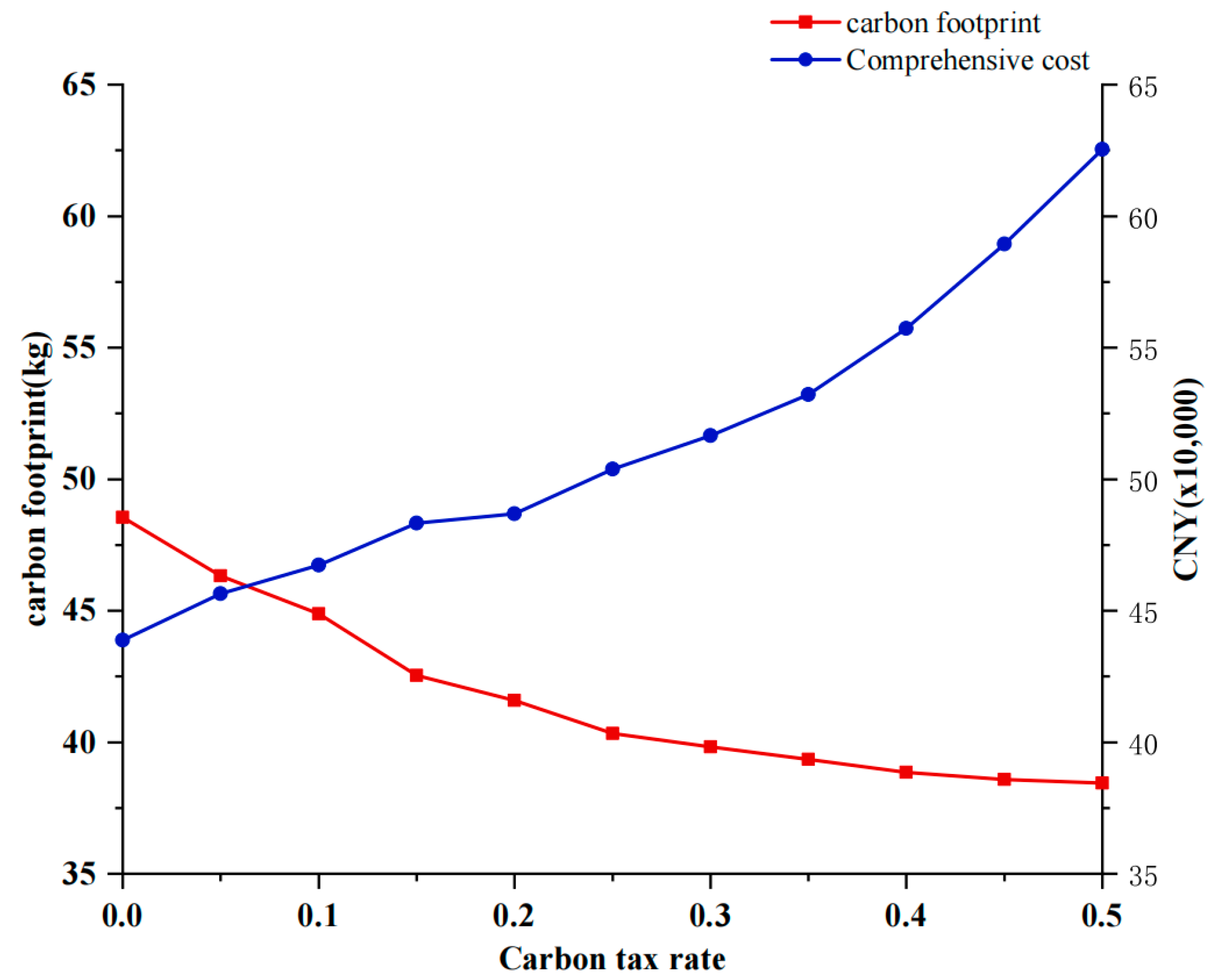
Container vessels require auxiliary motors for energy supply during berthing to maintain the necessary vessel operations and onboard facilities. Carbon emissions are also generated when the vessels are at berth in the port. Therefore, the carbon emissions of container vessels during the period between berthing and departure from the port must be considered when calculating the carbon tax cost.

$$Z_{CT}=\rho {·c}_{CT}·c_i{\sum }_{i\in V}{\sum }_{t\in T}{\sum }_{q\in Q}{\vartheta }_{itq}$$

(5)

Based on the above parameter definitions and cost definitions, ships and quay cranes in the planning period are taken as the study objects, and practical constraints, such as time, space, energy consumption and carbon tax, are considered. As a result, a mixed integer planning model is constructed with the objective of minimizing port operation and carbon tax costs. The objective function and constraints are as follows:

$$Min Z=Z_w+Z_d+Z_b+Z_p+Z_{CT}$$

(6)

$$b_i+l_i\le L\forall i\in V$$

(7)

$$b_j\ge b_i+l_i-M·\left({\delta }_{ij}-1\right)\forall i,j\in V, i\ne j$$

(8)

Constraint (7) stipulates that the actual berthing position of the vessel must be within the shoreline of the quay. Constraint (8) defines the relative berthing position relationship between different vessels.

$$y_i^b\ge y_i^a+{\theta }_i\forall i\in V$$

(9)

Constraint (9) indicates that there is a buffer time, ${\theta }_i$, to berth after the vessel’s expected arrival time.

$$y_j^b\ge y_i^d+M·\left({\epsilon }_{ij}-1\right) \forall i,j\in V, i\ne j$$

(10)

$${\delta }_{ij}+{\delta }_{ji}+{\epsilon }_{ij}+{\epsilon }_{ji}\ge 2 \forall i,j\in V, i\ne j$$

(11)

Constraints (10) and (11) define a sequential relationship between any two vessels in time and space, with no conflicts in the temporal and spatial dimensions.

$$Q_i^{min}{\tau }_{it}\le {\sum }_{q\in Q}{\vartheta }_{itq}\le Q_i^{max}{\tau }_{it} \forall i\in V,q\in Q$$

(12)

Constraint (12) defines a constraint on the number of quay crane jobs on board vessel $i$ at moment $t$.

$${\vartheta }_{itq}+{\vartheta }_{jtq}\le 1+M·\left({\epsilon }_{ij}+{\epsilon }_{ji}\right) \forall i,j\in V, i\ne j,q\in Q,t\in T$$

(13)

Constraint (13) limits quay crane service to one vessel at a time. When there exists a common berthing period for two vessels, no quay crane $q$ can serve both vessels $i$ and $j$ at the same time.

$${\sum }_{t\in T}\left({\sum }_{q\in Q}{\vartheta }_{itq}\left(\mu +{∆}_i^v\right){\gamma }^{{\sum }_{q\in Q}{\vartheta }_{itq}-1}\right)\ge \left(1+\beta \left|b_i-b_i^e\right|\right)\left(W_i^U+W_i^D\right)\forall i\in V,q\in Q,t\in T$$

(14)

In accounting for the uncertainty in quay crane operation efficiency, constraint (14) explicitly outlines that the quay crane operation efficiency during dynamic scheduling comprises both the average efficiency of quay crane operation and buffer efficiency. Simultaneously, it addresses the mutual interference among quay cranes during operation and considers the impact of a vessel deviating from the optimal berthing position. This approach aims to minimize the effects of uncertainties in quay crane operation time at the terminal.

$${\sum }_{i\in V}{\sum }_{q\in Q}\left({\vartheta }_{itq}+{\omega }_{itq}\right)+{\sum }_{q\in Q_R}{\phi }_{tq}\le Q\forall i\in V,q\in Q,t\in T$$

(15)

Constraint (15) defines the total crane amount constraints for the different states.

$${\sum }_{qϵQ}{\omega }_{itq}\ge Q_{i\left(t+1\right)}-Q_{it}\forall i\in V,q\in Q,t\in T$$

(16)

Constraint (16) denotes the number of dock cranes that move to vessel $i$ more at moment $t+1$ than at time $t$.

$$m+M\left({\vartheta }_{itm}+{\vartheta }_{jtn}+{\delta }_{ij}-3\right)\le n-1 \forall i,j\in V,i\ne j,m,n\in Q,m\ne n,t\in T$$

(17)

$${\vartheta }_{it\left(m-1\right)}-{\vartheta }_{itm}+{\vartheta }_{itn}\le 1 \forall i\in V,m,n\in Q,n\in \left[m+1,\right.\left.q\right)$$

(18)

Constraints (17) and (18) indicate that none of the quay cranes serving the same vessel or different quay cranes at the same moment may work crosswise and that the quay cranes serve sequentially on the shoreline.

$${\vartheta }_{itx}\le M\left(2-{\tau }_{it}+{\alpha }_{iy}-{\phi }_{ty}\right) \forall i\in V,y\in Q_1,x\in \left[1,\right.\left.y-1\right],t\in T$$

(19)

$${\vartheta }_{itx}\le M\left(3-{\tau }_{it}-{\alpha }_{iy}-{\phi }_{ty}\right)\forall i\in V,y\in Q_1,x\in \left[y+1,\right.\left.q\right],t\in T$$

(20)

Constraints (19) and (20) indicate the impact of a dock crane with a maintenance program on other dock cranes during the same time period.

$${r_q^{min}\le r}_q\le r_q^{max}\forall q\in Q_R$$

(21)

Constraint (21) defines the range of maintenance periods for quay cranes.

$$r_q\le t{\phi }_{tq}\le r_q+p_q\forall q\in Q_1,t\in \left[r_q^{min},r_q^{max}\right]$$

(22)

Constraint (22) defines the relation between the period experienced when the quay crane is in a maintenance state and the maintenance time.

$$M\left(1-{\vartheta }_{itq}\right)\ge {\phi }_{tq}\forall i\in V,q\in Q_1,t\in T$$

(23)

Constraint (23) defines the relationship between the work and maintenance status of a quay crane during the same period.

3.3. Adaptive Spiral Flight Dung Beetle Algorithm

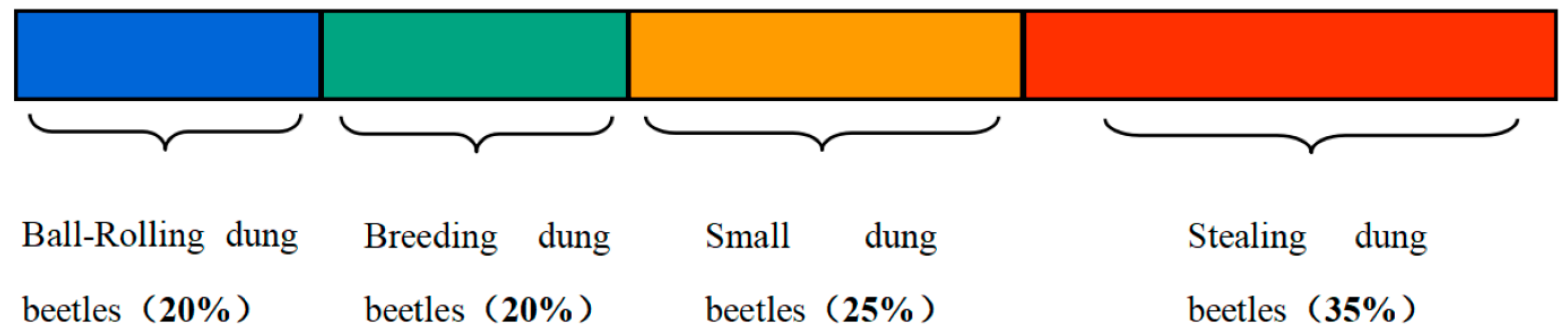
The dung beetle optimizer algorithm is a novel population intelligence optimization algorithm proposed by Xue et al. [28] in 2023, and which is inspired by the social behaviors of dung beetle populations, i.e., dung beetles’ ball-rolling, dancing, foraging, breeding, and stealing behaviors. Figure 2 shows the proportion of population species distribution in the DBO algorithm.

Rolling dung beetles explore space through two behavioral patterns: rolling dung balls and dancing. While rolling the dung ball, light is usually used as a guide to help the dung beetle to roll in a straight line. Its movement path is affected by the intensity of the light source, and the manner in which its position is updated while rolling the dung ball can be described as shown in Equation (24).

$$x_i^{t+1}=x_i^t+\alpha k{x}_i^{t-1}+b\left|x_i^t-x_{worst}\right|$$

(24)

where $x_{best}^t$ is the position information of the ith dung beetle at the tth iteration; $k$ is the deviation coefficient, $k\in \left(0\right.,\left.0.2\right]$; $b$ is a constant, $b\in \left(0\right.,\left.1\right)$; and $x_{worst}$ is the global worst position.

We use a probabilistic approach to set α to either 1 or −1. When $\alpha =1$, it indicates that the natural environment does not affect the original direction; when $\alpha =-1$, it indicates a deviation from the original direction—the dung beetle dances to obtain a new rolling direction when encountering an obstacle. The formula for its position update is shown in Equation (25).

$$x_i^{t+1}=\left\{\begin{array}{cc}{x}_i^t+\tan \theta \left|x_i^t-x_i^{t-1}\right|& ,\theta \ne 0,\frac{\pi }{2},\pi \\ x_i^t& ,\theta =0,\frac{\pi }{2},\pi \end{array}\right.$$

(25)

Dung beetles are notable for their ecological role, and they have a unique behavior of securing breeding offspring by rolling their feces into balls to a safe location.

$${Lb}^{*}=max\left(x_{best}^t·\left(1-R\right),Lb\right)$$

(26)

$${Ub}^{*}=min\left(x_{best}^t·\left(1+R\right),Ub\right)$$

(27)

In Equations (26) and (27), $x_{best}^t$ represents the current localized best position and ${Lb}^{*}$ and ${Ub}^{*}$ represent the upper and lower boundaries of the spawning area, respectively. $R=1-t/T_{max}$, and $T_{max}$ is the maximum number of iterations.

In the DBO algorithm, a female dung beetle determines the spawning area and then chooses a suitable breeding ball to lay her eggs. The algorithm determines that each female dung beetle can only lay one egg per iteration, and the boundary range of the spawning area changes dynamically with each iteration, which is mainly determined by the parameter R. The location of the breeding balls is also adjusted to adapt to the iteration process. As a result, the position of the breeding ball is also dynamically adjusted with the iteration process to adapt to the environmental changes, thus simulating the behavioral strategies of dung beetles in the natural environment and ensuring the offspring’s safety and the effective use of resources.

$$B_i^{t+1}=x_{best}^t+b_1\left(B_i^t-{Lb}^{*}\right)+b_2\left(B_i^t-{Ub}^{*}\right)$$

(28)

In Equation (28), $B_i^t$ denotes the position information of the ith breeding sphere at the tth iteration, and $b_1$ and $b_2$ represent two independent random vectors of size 1 × D. where ‘D’ represents the dimension of the optimization problem.

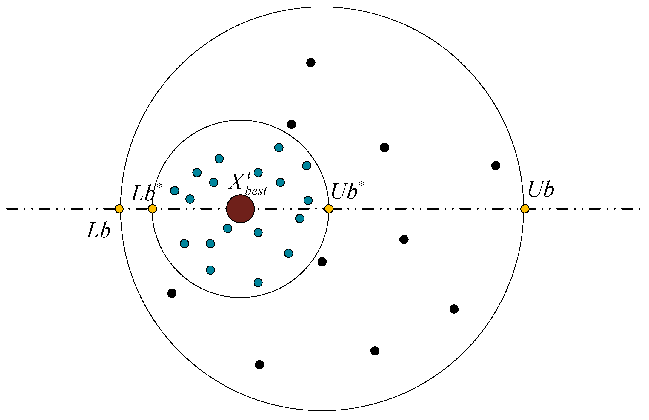
We introduce a boundary selection strategy to simulate the selection of the spawning region, as shown in Figure 3. The black dots indicate the position of the rolling dung beetle, while the current local optimal position $x_{best}^t$ is marked by a large brown circle, and the blue colored dots around $x_{best}^t$ indicate the breeding ball. In addition, yellow dots indicate the upper and lower limits of the boundary.

To simulate the process of small dung beetles searching for food in nature, we constructed a concept of an optimal foraging zone. The boundaries of this zone were set to locations that would guide the dung beetle to forage efficiently.

$${Lb}^l=max\left(x_{best}·\left(1-R\right),Lb\right)$$

(29)

$${Ub}^l=min\left(x_{best}·\left(1+R\right),Ub\right)$$

(30)

In Equations (29) and (30), $x_{best}$ is the global best position, and ${Lb}^l$ and ${Ub}^l$ are the lower and upper limits of the best foraging area, respectively.

Small dung beetle locations have been updated as follows:

$$x_i^{t+1}=x_i^t+C_1\left(x_i^t-L{b}^l\right)+C_2\left(x_i^t-U{b}^l\right)$$

(31)

In Equation (31), $C_1$ is a random number following a normal distribution and $C_2$ is a random vector within the range (0,1).

The stealing dung beetle does not steal from any arbitrary location but instead performs its stealing behavior near the best place to steal, i.e., near the globally optimal location. The location update rules for stealing dung beetles are as follows:

$$x_i^{t+1}=X^b+S·g·\left(\left|x_i^t-X^{*}\right|+\left|x_i^t-X^b\right|\right)$$

(32)

where $g$ is a random vector of size 1 × D following a normal distribution, $S$ denotes a constant, $X^b$ denotes the global best position, and $X^{*}$ denotes the current local best position.

In general, the DBO algorithm has fast convergence and high solution accuracy. Nevertheless, it grapples with drawbacks such as susceptibility to local optima and limited global exploration ability. The original DBO algorithm requires enhancements in both the exploration and exploitation phases. The proposed ASFDBO algorithm addresses this imbalance through improvements in the Bernoulli mapping strategy, variable spiral search strategy, Lévy flight strategy, adaptive weighting strategy, and Gauss–Cauchy hybrid variational perturbation strategy.

3.3.1. Chaotic Mapping Initializes the Population

Chaos mapping, an amalgamation of deterministic and stochastic approaches, is distinguished by its inherent characteristics of randomness and non-periodicity. Bernoulli mapping, a subtype of chaotic mapping, is frequently employed for the generation of chaotic sequences due to its nonlinear, ergodic, and random characteristics. In the realm of optimization, it replaces random numbers for population initialization, significantly influencing the algorithmic process. Studies, such as the work by Saito et al. [29], have demonstrated that Bernoulli mapping outperforms random numbers in achieving optimal results during the optimization searches. The research also underscores the suitability of Bernoulli mapping for chaotic population initialization, showcasing its traversal uniformity and convergence speed. Through well-designed experiments, Saito et al. [29] provided evidence supporting the use of Bernoulli mapping for the generation of initial populations in optimization algorithms. The distribution of chaotic sequences generated by Bernoulli mapping is depicted in Figure 4, further illustrating its effectiveness in this context.

Therefore, in this paper, Bernoulli mapping is used to initialize the position of dung beetle individuals. Firstly, the Bernoulli mapping relation is used to project the resulting values into the space of chaotic variables. Then, the resulting chaotic values are mapped into the initial space of the algorithm by a linear transformation. The specific expression of Bernoulli mapping is:

$$z_{k+1}=\left\{\begin{array}{cc}\frac{z_n}{1-\lambda }& ,0\le z_n\le 1-\lambda \\ \frac{z_n-\left(1-\lambda \right)}{\lambda }& ,1-\lambda \le z_n\le 1\end{array}\right.$$

(33)

where $\lambda$ is the mapping parameter, $\lambda \in \left(\mathrm{0,1}\right)$.

3.3.2. Variable Spiral Search Strategy

The whale optimization algorithm, commonly known as the WOA algorithm, draws inspiration from the distinctive feeding behavior of humpback whales. The spiral-up strategy in the WOA algorithm effectively improves the convergence of the algorithm to continue searching in the position near the individual. This strategy is incorporated into the dung beetle breeding ball formula and the small dung beetle foraging formula of the original dung beetle algorithm by adding the dynamic spiral parameter again so that the breeding ball position and the small dung beetle foraging are both in the form of a spiral within the search space. This expands the discoverer’s ability to explore the unknown region, helps the algorithm to jump out of a local optimum, and effectively improves the algorithm’s global search ability.

Dynamic spiral parameters in this paper are as follows:

$$u=e^{k·cos\left(\pi \left(1-\frac{i}{i_{max}}\right)\right)}$$

(34)

where the parameter k is generally taken as 5.

The improved formula for the position of the dung beetle breeding ball is as follows:

$$B_i^{t+1}=x_{best}^t+e^{ul}·\left(\mathit{cos}2\pi l\right)·b_1\left(B_i^t-L{b}^{*}\right)+e^{ul}·\left(\mathit{cos}2\pi l\right)·b_2\left(B_i^t-U{b}^{*}\right)$$

(35)

where $l$ represents a random number within the range $\left[-\mathrm{1,1}\right]$.

The improved formula for the foraging behavior of small dung beetles is as follows:

$$x_i^{t+1}={e^{ul}·\left(\mathit{cos}2\pi l\right)·x}_i^t+C_1\left(x_i^t-L{b}^l\right)+C_2\left(x_i^t-U{b}^l\right)$$

(36)

Analyzing the above formulas, it can be seen that the introduction of the variable spiral search strategy makes parameter u change continuously during the iteration process, which can dynamically adjust the scope of the spiral search. This is conducive to enhancing the flexibility of the search and improving the algorithm’s performance of the globally optimal search.

3.3.3. Adaptive Weighting and Lévy Flight Strategies

The adaptive weight is a crucial parameter in the dung beetle algorithm, necessitating adjustment. In the early iterations, a higher adaptive weight is employed to broaden the global search range, facilitating an extensive exploration for the global optimal solution. Conversely, in the later iterations, a smaller inertia weight is required to enhance the algorithm’s proficiency in utilizing the local area and preventing it from converging to a local optimal solution.

The adaptive weighting factors proposed in this paper are as follows:

$$\omega ={\omega }_{min}+\left({\omega }_{max}-{\omega }_{min}\right)·\mathit{sin}\left(\pi +\frac{\pi ·t}{2·t_{max}}\right)$$

(37)

Lévy flight [30] is a random walk process proposed by the French mathematician Lévy. Lévy flight randomly alternates between large and small steps, allowing for an algorithm to effectively jump out of a local optimum. The Lévy flight strategy is introduced into the stealing behavior of the stealing dung beetle, which perturbs the current optimal solution and strengthens the local escape ability.

The improved formula for the stealing behavior of dung beetles is as follows:

$$x_i^{t+1}=Lévy·X^b+S·g·\left(\left|x_i^t-X^{*}\right|+\left|x_i^t-{\omega ·X}^b\right|\right)$$

(38)

where $Lévy$ conforms to the Lévy distribution and satisfies $Lévy\left(\lambda \right)~u=t^{-\lambda }\left(1<\lambda \le 3\right)$. Due to the complexity of Lévy flights, they are usually modeled using the Mantegna algorithm [31], with the step size S given as follows:

$$S=\frac{u}{{\left|v\right|}^{1/\beta }}$$

(39)

In Equation (39), both $u$ and $v$ follow a normal distribution:

$$\begin{gathered} u~N\left(0,{\sigma }_u^2\right),v~N\left(0,{\sigma }_u^2\right) \\ \left\{\begin{array}{c}{\sigma }_u={\left\{\frac{\Gamma \left(1+\beta \right)·\mathit{sin}\left(\frac{\pi \beta }{2}\right)}{\Gamma \left(\frac{1+\beta }{2}\right)·\beta ·2^{\frac{\beta -1}{2}}}\right\}}^{1/\beta }\\ {\sigma }_v=1\end{array}\right. \end{gathered}$$

(40)

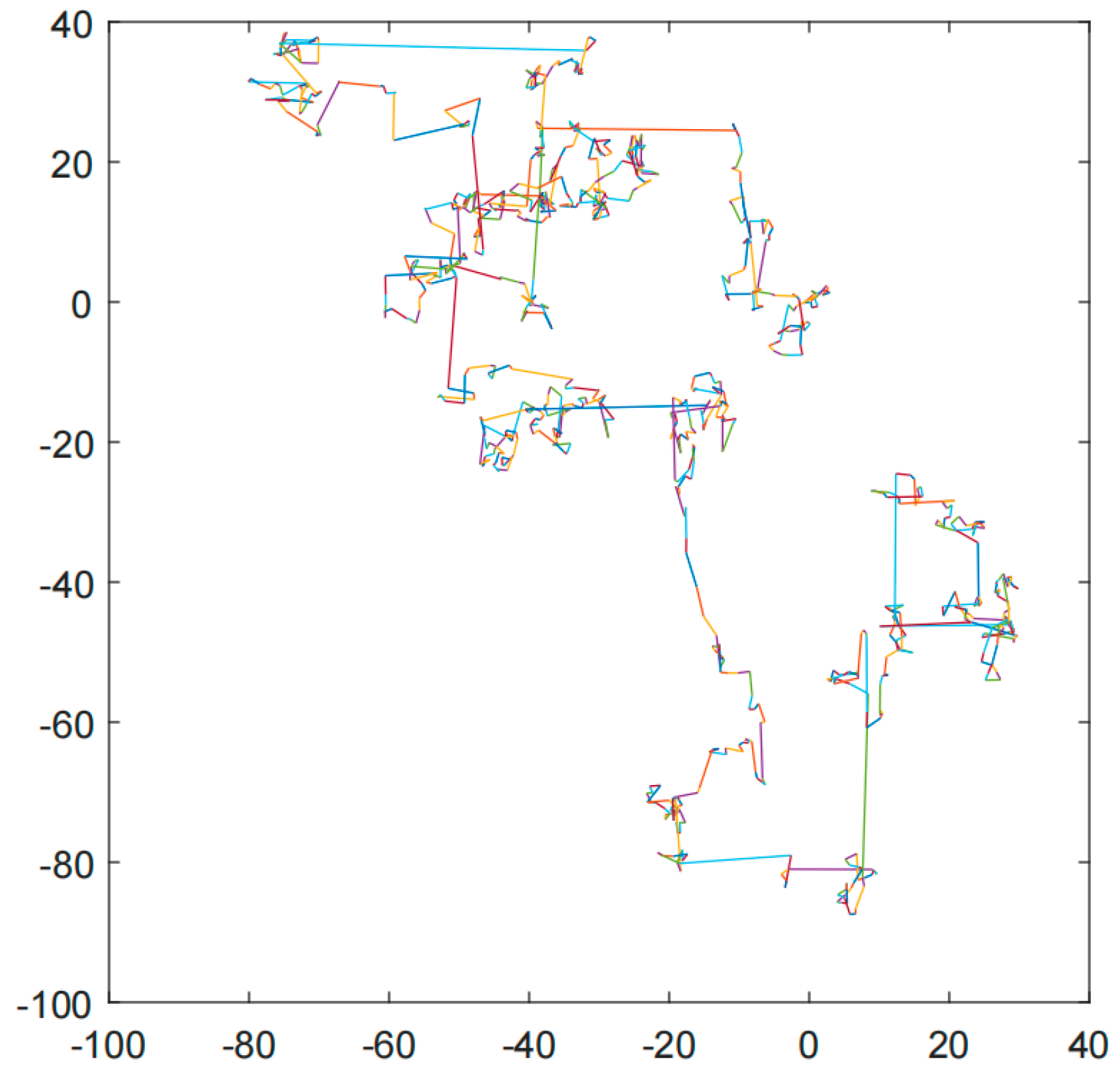
Figure 5 shows the simulation of a 2D planar Lévy flight in Matlab using Mantegna’s method; from the simulation, the paths of the graphs are indeed in line with the characteristics of Lévy flights in terms of their lengths and shorter lengths, and Mantegna’s method of generating stochastic steps that obey a Lévy distribution with a normal distribution is reliable.

3.3.4. Gauss–Cauchy Mixed Variants Perturbation

In the later iterations of the basic dung beetle algorithm, individual dung beetles assimilate rapidly, causing the population to aggregate near the current optimal position. This position’s value approximates the optimal solution. However, the current optimal position is not a globally optimal point. In that case, the dung beetle population tends to concentrate its search around this position, leading to a failure in discovering the optimal position and resulting in a stagnant search. To address this issue, a variational perturbation operation is commonly employed to disturb individuals, thereby increasing population diversity and allowing them to move beyond local optima [32]. The mutation perturbation operation enhances the population diversity of dung beetles, enabling the algorithm to escape local optima and explore other regions of the solution space. This exploration continues until the global optimum solution is ultimately found. Introducing variation operators in intelligent optimization algorithms augments population diversity and prevents the algorithm from becoming stuck in a local minima [33]. Among the commonly used variation operators, Cauchy and Gauss variations have advantages and disadvantages. The Cauchy variant provides a more extensive search range than the Gauss variant. However, its step size, being too large, may cause it to jump away from the optimum, resulting in poorer progeny [34]. On the other hand, the Gauss variant exhibits good search ability within a small range [35], due to its capability to produce smaller variant values with a higher probability.

$$x_i^{new}\left(t\right)=x_i\left(t\right)·\left[1+{\beta }_{1}Cauchy\left(\mathrm{0,1}\right)+{\beta }_{2}Gauss\left(\mathrm{0,1}\right)\right]$$

(41)

In Equation (41), $Cauchy\left(\mathrm{0,1}\right)$ is a random number obeying the Cauchy distribution; $Gauss\left(\mathrm{0,1}\right)$ is a random number obeying the Gauss distribution; $x_i^{new}\left(t\right)$ is the position after the mutation, ${\beta }_1=T_{max}$, ${\beta }_2=1-T_{max}$; and the weight coefficients of the mutation operator ${\beta }_1$, ${\beta }_2$ are gradually changed in a one-dimension and linear manner, a manner which is aimed at guaranteeing that the perturbation of each iteration is equilibrium smoothed.

Early in the iteration of the algorithm, the Cauchy variation plays a greater role, expanding the search range of the population. The Gauss variation plays a major role in allowing individuals to search in a small area, enhancing the local search ability of the population, and allowing the algorithm to converge quickly.

3.3.5. Parameterization of the ASFDBO Algorithm

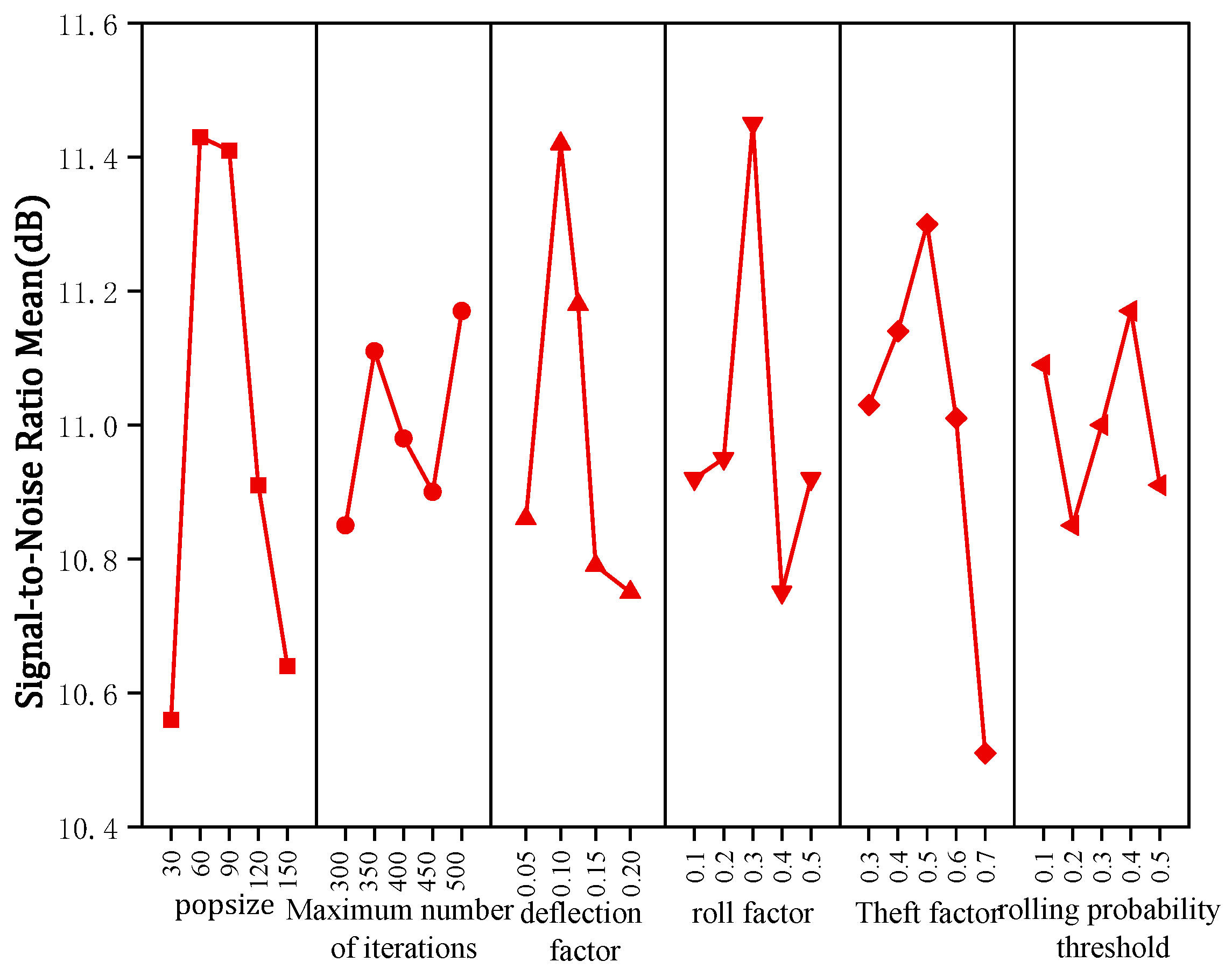
In this study, the Taguchi method is used to determine the algorithm parameters, and the signal-to-noise ratio (SNR) is utilized to evaluate the algorithm’s performance under different combinations of parameters. During the implementation of the algorithm, parameters such as popsize, maximum number of iterations ($T_{max}$), deflection coefficient ($k$), roll coefficient ($b$), steal coefficient ($S$), and roll probability threshold ($\lambda$) are required to be set.

Figure 6 shows the main effect plot of the signal-to-noise ratio of the algorithm parameters generated in Minitab 21.4 software. Based on the analysis results, we determined the following values for each parameter: popsize is 90, maximum number of iteration generations ($T_{max}$) is 500, deflection coefficient ($k$) is 0.1, roll coefficient ($b$) is 0.3, stealing coefficient ($S$) is 0.5, and roll probability threshold ($\lambda$) is 0.4.

3.3.6. ASFDBO Algorithm Validation

To assess the efficacy of the ASFDBO algorithm, a comparative analysis is conducted with other swarm intelligence optimization algorithms, namely the whale optimization algorithm (WOA) [36], sparrow search algorithm (SSA) [37], grey wolf optimization (GWO) [38] and basic dung beetle optimization algorithm (DBO). All algorithms share standard settings with a maximum number of iterations (T) set at 500. Parameters for each algorithm are strictly adhered to as per the original text.

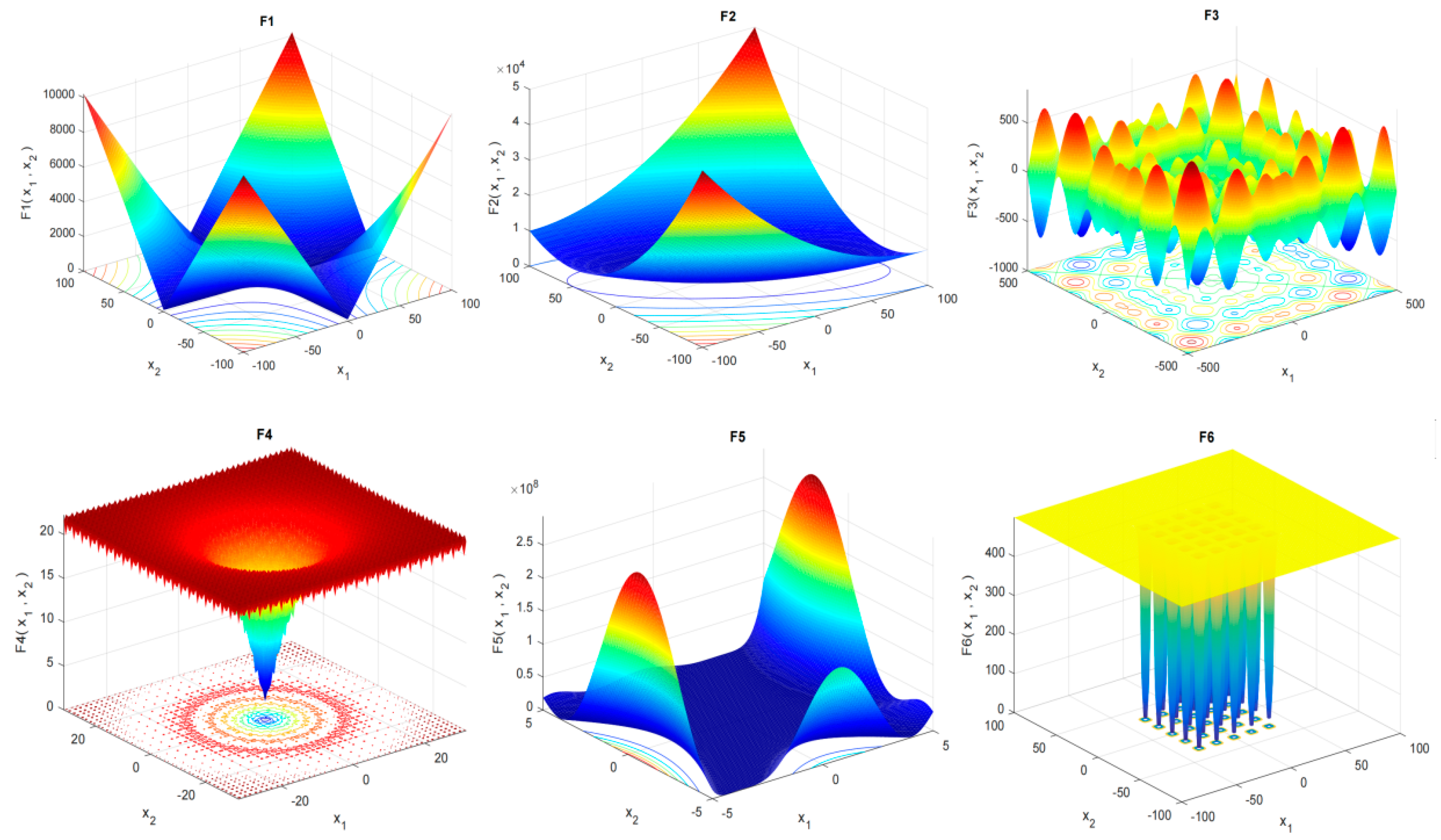
The six standard test functions in

Table 3. Test functions.

Test Functions	Dimension	Range	Min
$f_1={\displaystyle \sum _{i=1}^n}\left|x_i\right|+{\prod }_{i=1}^n\left|x_i\right|$	30	[−10, 10]	0
$f_2={\displaystyle \sum _{i=1}^n}{\left({\displaystyle \sum _{j=1}^i}{x}_j\right)}^2$	30	[−100, 100]	0
$f_3={\displaystyle \sum _{i=1}^n}-x_i\sin \left(\sqrt{\left|x_i\right|}\right)$	30	[−500, 500]	−12,569.5
$f_4=-20exp\left(-0.2\sqrt{\frac{1}{n}}{\displaystyle \sum _{i=1}^n}{x}_i^2\right)-exp\left(\frac{1}{n}{\displaystyle \sum _{i=1}^n}\cos \left(2\pi x_i\right)\right)+20+e$	30	[−32, 32]	0
$f_5=\left[1+{\left(X_1+X_2+1\right)}^2\left(19-14X_1+3X_1^2-14X_2+6X_1{X}_2+3X_2^2\right)\right]\times \left[30+{\left(2X_1-3X_2\right)}^2\times \left(18-32X_1+12X_1^2+48X_2-36X_1{X}_2+27X_2^2\right)\right]$	2	[−2, 2]	3
$f_6={\left[\frac{1}{500}+{\displaystyle \sum _{j=1}^{25}}\frac{1}{j+{\sum }_{i=1}^2{\left(x_i-a_{ij}\right)}^6}\right]}^{-1}$	2	[−65, 65]	0.998

were used for performance testing. Figure 7 shows a three-dimensional plot of the functions of Table 3. Of these functions, $f_1$−$f_2$ are high-dimensional single-peak functions, each featuring only one global optimal solution. These functions serve to assess the algorithm’s developmental capabilities. $f_3$−$f_4$ are high-dimensional multi-peak functions characterized by one global optimal solution and multiple local optimal solutions. $f_5$−$f_6$ are fixed dimensional multi-peak functions. These functions evaluate the algorithm’s proficiency in global search and local escape abilities.

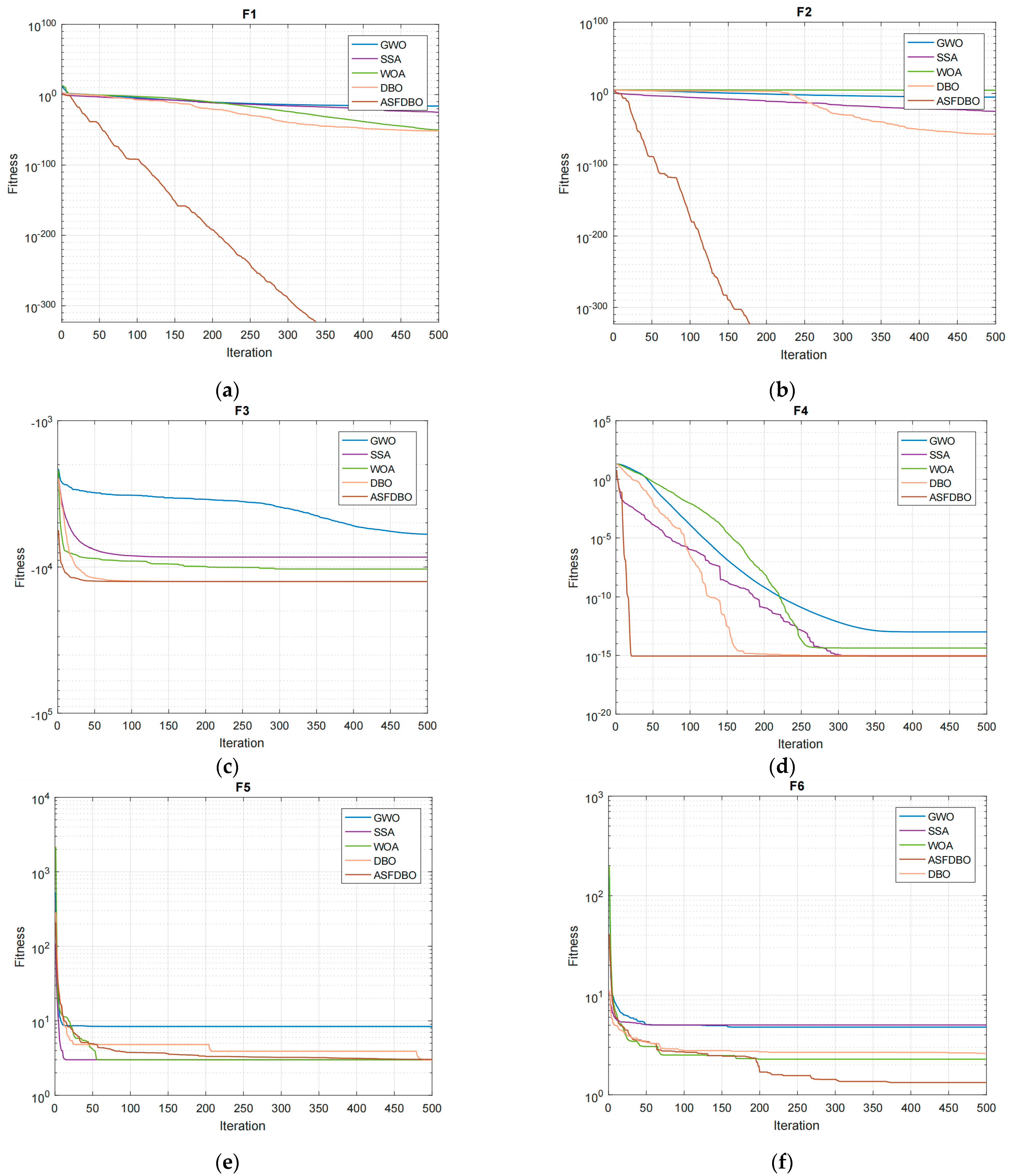
The criteria for evaluating the optimization performance of the algorithm consist of the optimal value, average value, and standard deviation, calculated from 20 optimization results. The optimal value signifies the algorithm’s accuracy, while the average value and standard deviation reflect its stability. The optimization results and convergence curves can be found in

Table 4. Algorithm optimization results.

Function	Algorithm	Best	Average	St. dev
$f_1$	GWO	$1.21\times {10}^{-17}$	$8.03\times {10}^{-17}$	$5.79\times {10}^{-17}$
	SSA	$3.54\times {10}^{-214}$	1.75$\times {10}^{-27}$	$9.60\times {10}^{-27}$
	WOA	$2.29\times {10}^{-57}$	$4.88\times {10}^{-50}$	$2.31\times {10}^{-49}$
	DBO	$1.15\times {10}^{-79}$	$1.77\times {10}^{-56}$	$9.70\times {10}^{-56}$
	ASFDBO	$0$	$0$	$0$
$f_2$	GWO	$3.92\times {10}^{-8}$	$2.67\times {10}^{-5}$	$6.15\times {10}^{-5}$
	SSA	$2.28\times {10}^{-221}$	$9.33\times {10}^{-24}$	$5.11\times {10}^{-23}$
	WOA	$2.24\times {10}^2$	$5.01\times {10}^2$	$1.00\times {10}^2$
	DBO	$9.42\times {10}^{-154}$	$8.62\times {10}^{-58}$	$4.72\times {10}^{-57}$
	ASFDBO	$0$	$0$	$0$
$f_3$	GWO	$-7.46\times {10}^3$	$-6.12\times {10}^3$	$6.30\times {10}^2$
	SSA	$-9.64\times {10}^3$	$-8.50\times {10}^3$	$6.51\times {10}^2$
	WOA	$-1.25\times {10}^4$	$-1.06\times {10}^4$	$1.70\times {10}^3$
	DBO	$-1.25\times {10}^4$	$-1.25\times {10}^4$	$4.71\times {10}^1$
	ASFDBO	$-1.25\times {10}^4$	$-1.25\times {10}^4$	$6.27\times {10}^{-1}$
$f_4$	GWO	$7.54\times {10}^{-14}$	$9.88\times {10}^{-14}$	$1.83\times {10}^{-14}$
	SSA	$8.88\times {10}^{-16}$	$8.88\times {10}^{-16}$	$0$
	WOA	$8.88\times {10}^{-16}$	$4.32\times {10}^{-15}$	$2.71\times {10}^{-15}$
	DBO	$8.88\times {10}^{-16}$	$1.00\times {10}^{-15}$	$6.48\times {10}^{-16}$
	ASFDBO	$8.88\times {10}^{-16}$	$8.88\times {10}^{-16}$	$0$
$f_5$	GWO	$3.00\times {10}^0$	$3.00\times {10}^0$	$4.60\times {10}^{-5}$
	SSA	$3.00\times {10}^0$	$5.70\times {10}^0$	$8.24\times {10}^0$
	WOA	$3.00\times {10}^0$	$3.00\times {10}^0$	$1.23\times {10}^{-4}$
	DBO	$3.00\times {10}^0$	$3.90\times {10}^0$	$4.93\times {10}^0$
	ASFDBO	$3.00\times {10}^0$	$3.00\times {10}^0$	$1.38\times {10}^{-7}$
$f_6$	GWO	$9.98\times {10}^{-1}$	$4.75\times {10}^0$	$4.40\times {10}^0$
	SSA	$9.98\times {10}^{-1}$	$5.41\times {10}^0$	$5.52\times {10}^0$
	WOA	$9.98\times {10}^{-1}$	$2.90\times {10}^0$	$2.62\times {10}^0$
	DBO	$9.98\times {10}^{-1}$	$1.49\times {10}^0$	$1.12\times {10}^0$
	ASFDBO	$9.98\times {10}^{-1}$	$1.33\times {10}^0$	$7.98\times {10}^{-1}$

and Figure 8. The results show that, for the single-peak functions $f_1$ and $f_2$, the ASFDBO algorithm outperforms the other algorithms in all three evaluation criteria, which fully reflects the solid local search ability and stability of ASFDBO. For the multi-peak functions $f_3$ and $f_4$, where the function $f_3$ is the most complex and has many minima, only the optimal convergence values and average convergence accuracies of the DBO algorithm and the ASFDBO algorithm reach the theoretically optimal solution, but the ASFDBO is better than the DBO. As for the fixed-dimensional multi-peak test functions, $f_5$ and $f_6$, the average convergence accuracies and standard deviations of the ASFDBO algorithm are ranked first, indicating that the ASFDBO algorithm can balance the exploration ability and exploitation ability well. Analyzing the convergence curve in Figure 8, The ASFDBO algorithm demonstrates a higher convergence accuracy than the SSA algorithm, known for its robust global search capability. This indicates that the ASFDBO algorithm excels in global search proficiency relative to other algorithms. The ASFDBO algorithm consistently breaks free from locally optimal solutions multiple times, reaching more optimal solutions and showcasing its remarkable ability to escape local areas. Simultaneously, the DBO algorithm converges more rapidly than others, yet the ASFDBO algorithm surpasses its convergence accuracy and speed. This substantiates that the ASFDBO algorithm effectively balances the exploration and development abilities of the algorithm.

In order to verify the effectiveness and practical applicability of the ASFDBO algorithm in the model of this paper, we chose the traveling salesman problem (TSP), which is the same NP-hard problem as the model of this paper. We also chose the welded beam design optimization problem, an engineering design problems, for verification. In the TSP problem, we chose the eil51, eil76, and ch130 instances for the relevant tests, and the test results are summarized in

Table 5. TSP optimization results.

TSP Example	Optimal Solution	Algorithm	Best	${\mathit{\delta }}_{\mathit{r}}$/%
eil51	426	GWO	432.57	1.54
		SSA	428.74	0.64
		WOA	431.48	1.28
		DBO	429.31	0.77
		ASFDBO	426	0
eil76	538	GWO	554.34	3.04
		SSA	549.63	2.16
		WOA	556.72	3.48
		DBO	548.31	1.92
		ASFDBO	540.78	0.51
ch130	6110.86	GWO	6589.22	7.83
		SSA	6289.28	2.92%
		WOA	6549.30	7.17%
		DBO	6334.57	3.67
		ASFDBO	6166.36	0.91

. ${\delta }_r$ is the relative error between the optimal value and the known optimal solution. Each algorithm is run for 10 instances at the corresponding instance.

As can be learned from Table 5, the simulation results based on the three TSP instances show that ASFDBO improves its solution quality by an average of 78% concerning the DBO algorithm. In the small-scale examples, ASFDBO can find the optimal solution. ASFDBO can still approach the optimum and outperform the DBO algorithm and other swarm intelligence algorithms as the example size increases. This shows that ASFDBO can find high-quality, stable solutions in different example sizes. As a result, the algorithm has better stability and robustness and is suitable for solving NP-hard problems with high complexity.

The goal of welded beam design is to minimize the cost of welded beams, and the main optimization variables are the weld thickness, h; the bar thickness, b; the length of the connected portion of the bar, l; and the height of the bar, t. As seen in the results of the comparison of the ASFDBO with the WBD problem in

Table 6. Comparative results of ASFDBO on WBD issues.

Algorithm	Variable’s Optimal Value				Cost Optimization
	$\mathit{h}$	$\mathit{l}$	$\mathit{t}$	$\mathit{b}$
GWO	0.20060	3.34667	9.03847	0.20577	1.7009
SSA	0.18256	3.71989	9.03662	0.20573	1.7219
WOA	0.20415	3.34888	9.43561	0.20128	1.7358
DBO	0.20194	3.27563	9.31635	0.20442	1.7304
ASFDBO	0.20520	3.26260	9.04033	0.20602	1.6985

, in engineering design optimization, the ASFDBO algorithm improves solution quality by 1.84% compared with the DBO algorithm. Furthermore, the ASFDBO algorithm outperforms others, proving its remarkable effectiveness in addressing engineering design optimization challenges.

3.4. Algorithm Flow and Steps for Problem-Solving

According to the characteristics of the mathematical model in this paper, the actual number coding is chosen, as shown in Figure 9.

The first three layers indicate the vessel’s berth stopping position, berthing time, and the number of cranes assigned to the vessel. The fourth layer indicates the crane number of the leftmost service of the vessel. The fifth and sixth layers are slack variables for arrival time and operational efficiency, respectively.

Figure 10 shows the flow chart of the algorithm ASFDBO.

The steps for the solution are as follows:

(1)

Initialize ASFDBO algorithm parameters, including total number of dung beetles, $N$; spatial search dimension, $D=2d-1$; and maximum number of iterations, $T_{max}$. Depending on the specific problem, determine the number of rolling dung beetles, breeding dung beetles, small dung beetles and stealing dung beetles, as well as the deflection coefficient ($k$), roll coefficient ($b$), steal coefficient ($S$), and roll probability threshold ($\lambda$), etc.

(2)

Initializing dung beetle population locations using Bernoulli mapping chaotic.

(3)

The objective function value for each dung beetle in the population is calculated to obtain the global optimal position, $X_{best}$, corresponding to the minimum objective function value and the worst position, $X_{worst}$, corresponding to the maximum objective function value.

(4)

Update the location of the rolling dung beetle. If the individual dung beetle belongs to the ball-rolling dung beetle species, a probabilistic method is used to determine whether the individual’s next behavior will continue to be ball-rolling or become dancing. Given a rolling probability threshold $\lambda$, let $\delta =rand\left(1\right)$; if $\delta <0.9$, then let $\eta =rand \left(1\right)$, $\alpha =1(\eta >\lambda )$ or $\alpha =-1(\eta \le \lambda )$. Update the position according to equation (24). Otherwise, update the position according to Equation (25), then determine the current local optimum position

(5)

Update the location of the other three subpopulations of dung beetles. If the dung beetle belongs to the species of breeding dung beetles, then update the position according to (35).

If the individual dung beetle belongs to the small dung beetle species, then update the position according to (36).

If the individual belongs to the stealing dung beetle species, then update the position according to Equation (38).

(6)

Calculate the objective function value of the dung beetle individuals at the current location body to obtain the global objective function value corresponding to the smallest objective function value’s optimal position, $X_{best}$.

(7)

Perturb the current optimal solution using the Gauss–Cauchy variational perturbation strategy to generate a new solution.

(8)

Determine whether the iteration termination condition is satisfied. If the number of iterations reaches $T_{max}$, the iteration terminates and outputs the global optimal position, $X_{best}$ (the minimum integrated cost of berth and crane scheduling); otherwise, skip to step (4) for the next iteration.

4. Numerical Experiments

In this study, the algorithm is validated through numerical experiments executed on an MSI computer system featuring a 2.50 GHz Intel Core i5-12400 CPU and 16 GB RAM located in Hangzhou, China. MATLAB 2016b is employed as the software platform for conducting the experiments.

4.1. Algorithmic Parameterization

Our experimental subject is a quay with a shoreline length of 1000 m. There are ten quay cranes whose initial positions correspond to specific berth segments; for example, quay crane 1 is positioned in the berth segment of 0–100 m, quay crane 2 in the 100–200 m segment, and so forth. Considering quay crane operation efficiency uncertainty, the expected value is set to $\mu =10$ TEU/h. $\gamma$ is 0.9.

With reference to the standard of carbon tax levied by countries around the world, $\rho =$0.22 CNY/t, $c_{CT}=$45.88 kg/min, $c_w$ is 10, $c_p$ is 50 and $c_b$ is 0.01. The penalty cost per hour for vessel delays in leaving the harbor is 10% of the length $l_i$.

Table 7. Range of parameters.

Symbol	Definition	Range
$l_i$	Length of vessels to be dispatched	$U\left(\mathrm{120,360}\right)\bigcap Z$
$b_i^e$	Expected berth positions of vessels to be dispatched	$U\left(0,L\right)\bigcap Z$
$Q_i$	Designated quay crane number	$U\left(1,N_Q+1\right)\bigcap Z$
$W_i^U$	Number of containers exported from vessels	$U\left(\mathrm{100,300}\right)\bigcap Z$
$W_i^D$	Number of containers imported by vessels	$U\left(0.7W_i^U,1.3W_i^U\right)\bigcap Z$
$y_i^a$	The anticipated time of vessel arrival	$U\left(\mathrm{0,72}\right)$
${ED}_i$	The anticipated departure time of the vessel	$U\left(\mathrm{1.1,1.5}\right)\times \frac{\left(W_i^U+W_i^D\right)}{Q_i^{min}}+y_i^a$
$Q_i^{min}$	Minimum number of quay cranes allocated	$U\left(\mathrm{2,4}\right)\bigcap Z$
$Q_i^{max}$	Maximum number of quay cranes allocated	$U\left(Q_i^{min},6\right)\bigcap Z$
$p_q$	Quay cranes are scheduled to require maintenance time	$U\left(\mathrm{2,6}\right)\bigcap Z$
$r_q^{min}$	Earliest start time for maintenance	$U\left(\mathrm{0,66}\right)\bigcap Z$
$r_q^{max}$	Latest start time for maintenance	$U\left(r_q^{min},66\right)\bigcap Z$
${\theta }_i^s$	Actual arrival time of vessels in the sample	$N\left(y_i^a,1.5\right)$
$v_i^s$	Actual working efficiency of quay cranes in the sample	$N\left(\mu ,1\right)$

provides an overview of the parameter ranges for the dispatched vessels. Define the symbol $U$ to be a uniform distribution and the symbol $Z$ to be the set of integers.

4.2. Dispatch Solution Analysis

To evaluate the effectiveness of the ASFDBO algorithm, we randomly generate an instance of size 15. The scheduling solutions for these instances using the ASFDBO algorithm are illustrated in Figure 11. The white rectangles and the labels next to them in the ship berthing work Gantt chart represent the ship and the number of the crane serving it, and the white shaded rectangles represent the cranes under maintenance. Different color rectangles in the crane work and maintenance Gantt chart represent different vessels, and the length of the rectangles is the working time of the vessel. We can obtain information about all of the dispatched vessels and details regarding the quay cranes with maintenance plans. For example, vessel 3 berths at berth section 160–140 m at time 10.5 and is served by quay crane vessels 1 to 5, it completes loading and unloading and leaves the quay at time 20. Quay crane 6 completes loading and unloading and returns to the berth section corresponding to its initial position for maintenance work at time 16.5, completes maintenance work at 19.5, and moves to berth section 540–755 m at time 24.5. It can be easily noticed that all of the binding restrictions were not violated. All vessels were berthed within the length of the quay crane. The quay cranes with maintenance schedules moved to the berth segments corresponding to their initial positions in order to perform maintenance work during their maintenance schedule time. There were no vessels in the corresponding berth segments to perform berthing tasks, and there was no work crossover between quay cranes in other berth segments during the maintenance period. In summary, the ASFDBO algorithm produces feasible scheduling solutions.

4.3. Scheduling Environmental Strategy Benefits Analysis

In order to evaluate the effectiveness of each improvement strategy of the ASFDBO algorithm, we designed four different algorithmic experiments in two scenarios of size 10 and 15, as follows: algorithm without variational spiral search strategy (NSS-DBO), algorithm without adaptive weights and Lévy flight mechanism (NFL-DBO), algorithm without Gauss–Cauchy hybrid variational perturbation strategy (NGC-DBO), and the base algorithm without considering any improvement strategy (DBO).

Figure 12 illustrates the objective function value curves obtained by iterating the ASFDBO, NSS-DBO, NFL-DBO, NGC-DBO, and DBO algorithms on randomly generated instances of sizes 10 and 15. Through in-depth analyses of the iterative curves of each algorithm, we find that the ASFDBO algorithm, incorporating the variable spiral search strategy, adaptive weighting factor, Lévy flight strategy, and Gauss–Cauchy mixed variants perturbation strategy, not only demonstrates excellent local escape ability but also significantly outperforms the pre-improved algorithms in terms of convergence accuracy and global search ability. Notably, ASFDBO achieves a significant reduction of about 47% in the objective function value compared with the DBO algorithm, highlighting its excellent optimization performance.

Figure 13 shows the carbon emission iteration curves obtained by the ASFDBO, NSS-DBO, NFL-DBO, NGC-DBO, and DBO algorithms on instances of sizes 10 and 15. Through in-depth analyses of the iterative curves of each algorithm, it is found that the ASFDBO algorithm significantly reduces carbon emissions by about 46% compared with the DBO algorithm, highlighting the superior performance of the ASFDBO algorithm in reducing carbon emissions.

4.4. Carbon Tax Rate Impact Analysis

According to the General Rules for Calculation of Comprehensive Energy Consumption and the Greenhouse Gas and Emission Inventory, the average low-level heating capacity of fuel oil is 41,816 kJ/kg, the standard coal conversion factor is 1.4286 kgce/kg, the carbon content per unit of calorific value is 21.1, and the carbon oxidation rate is 0.98. From this, a carbon dioxide emission factor is considered 3.1705 kg. It is estimated that a standard 100 m container vessel requires 30 tons of fuel oil to run its auxiliary motor for 24 h during berthing, equivalent to 20.1 kg of fuel oil per minute. Considering that the average density of fuel oil is 0.72 kg/L, a vessel’s fuel consumption using fuel-powered auxiliary motors during berthing would result in 45.88 kg of CO₂ emissions per minute of fuel oil consumption. Carbon emission factors for vessels can be converted from the corresponding vessel lengths.

At an arithmetic scale of 15, we will explore the effects of different tax rates on carbon emissions and the comprehensive costs of the dispatch program. When substituting the tax rate into the model’s objective function in order to to solve with a considertion of carbon tax, the calculation results shown in

Table 8. Impact of different tax rates on carbon emissions and integrated costs.

Carbon Tax Rate	Carbon Footprint (kg)	Carbon Tax Costs	Comprehensive Cost
0	485,517	0	438,825
0.05	463,322	23,166.1	456,532
0.1	448,852	44,885.2	467,282
0.15	425,361	63,804.15	483,324
0.20	415,835	83,167	486,791
0.25	403,310	100,827.5	503,764
0.30	398,243	119,472.9	516,473
0.35	391,524	137,033.4	532,210
0.4	383,521	153,408.4	557,362
0.45	379,837	170,926.6	589,321
0.5	376,399	188,199.5	625,310

are obtained.

As shown in Figure 14, as the carbon tax rate $\rho$ increases, the comprehensive cost of the container port keeps increasing, and, conversely, the carbon emissions of the container terminal scheduling scheme decrease with the increase of the tax rate. It is worth noting that, when the value of carbon tax rate k is in the range of 0–0.3, the carbon emission decreases significantly with the increase of the tax rate. Additionally, the carbon emission rate decreases by 87,274 kg, with an average decrease rate of 2.99%. When the carbon tax rate $\rho$ is more significant than 0.3, carbon emissions with the tax rate increase the rate of decline slowly, with an average rate of decline of 1.37%. The container port berths and cranes scheduling program comprehensive cost change trend is just the opposite; as the carbon tax rate increases, its increase also increases. Therefore, evaluating the carbon emissions and comprehensive costs of scheduling optimization scenarios under different tax rates can help port authorities and policymakers to more comprehensively understand the ecological benefits and economic costs that may be brought about by implementing the scenarios so that they can make more informed decisions. By setting a reasonable carbon tax rate for port operations, carbon emissions from the port can be significantly reduced while increasing operating costs by a small amount. This comprehensive assessment can help optimize port operations and balance economic benefits and environmental sustainability.

5. Conclusions and Future Work

In this paper, a new model for collaborative berth and quay crane scheduling is proposed for uncertain scheduling environments, taking into account the cost of carbon tax due to carbon emissions in the comprehensive cost of container port scheduling scenarios. The model integrates several factors, including uncertain vessel arrival times, the imprecise operational efficiency of quay cranes, the interference between operations, and the maintenance schedules of quay cranes. To address this model, we design an adaptive spiral flight dung beetle optimization algorithm. The algorithm incorporates multiple strategies: variable spiral search, adaptive weighting, the Lévy flight mechanism, and a Gauss–Cauchy mixed-variant perturbation approach. We validated the ASFDBO algorithm, demonstrating its superior global search and local escape capabilities compared with other widely used intelligent algorithms.

In numerical experiments, we initially validate the feasibility and effectiveness of the ASFDBO algorithm using a sample size of 15. By scrutinizing the vessel scheduling Gantt chart and the quay crane work Gantt chart, we found that the algorithm can generate feasible cooperative scheduling plans for berths and quay cranes. Subsequently, we experimentally compared each of the enhanced strategies in the ASFDBO algorithm with the unimproved DBO algorithm, with all algorithms executed under the same sample conditions. Algorithm iteration plots show that the combination of multiple strategies significantly improves the global search accuracy of the algorithm. The model objective function value of the ASFDBO algorithm is reduced by about 47% compared with the original algorithm, with a corresponding reduction in carbon emissions of about 46%. Finally, we investigate the effect of different carbon tax rates on the optimization of joint scheduling. The results show that evaluating carbon emissions and comprehensive costs of dispatch optimization schemes under different tax rates can help port management and decision-makers keep a more comprehensive understanding of the possible ecological benefits and economic costs of scheme implementation. By setting a reasonable carbon tax rate for port operations, carbon emissions from the port can be significantly reduced, while operating costs increase by a small amount. This comprehensive assessment can help optimize port operations and balance economic benefits and environmental sustainability, providing more informed guidance for future decision-making.

There are several areas in which future research can be conducted to further the understanding and efficiency of port management systems. First, research on dynamic quay crane configurations will be a focus of attention. This implies that cranes can be reconfigured and serve other vessels before the current vessel leaves the port, thus significantly improving crane utilization. Therefore, subsequent research can improve the existing model by introducing dynamic elements to better respond to real-time demand changes.

In addition, future research could further explore the berth and crane scheduling problem between multiple terminals. This area of research could consider resource sharing, operational coordination, and optimal scheduling strategies among different terminals in order to maximize the benefits and minimize the carbon emissions of the entire port system. This comprehensive research will provide theoretical and methodological support for the building of a more innovative and sustainable port management system.

Finally, future research must explore how the ASFDBO algorithm can be applied to port operations. This involves technical requirements regarding system integration, data management, and port operators’ and shipping companies’ acceptance of ASFDBO algorithms. At the same time, concerns about data privacy protection are also essential factors to consider. In this process, it is necessary to clarify the parameters of the scheduling program with port operators and shipping companies. Meanwhile, in the face of the changing demands of low-carbon environment and carbon emission policies, it is necessary to determine the optimal parameters of the algorithms and evaluate whether the algorithms can maintain good robustness under changing scheduling scales and scheduling time windows. Therefore, future research should address these challenges in order to ensure the successful application of the ASFDBO algorithm in port operations and make a more significant contribution to the efficiency and sustainability of port operations.

References

1. Li, X.; Tan, X.; Wu, R.; Xu, H.; Zhong, Z.; Li, Y.; Zheng, C.; Wang, R.; Qiao, Y. Paths for Carbon Peak and Carbon Neutrality in Transport Sector in China. Strateg. Study CAE 2021, 23, 15–21. [Google Scholar] [CrossRef]
2. Bierwirth, C.; Meisel, F. A survey of berth allocation and quay crane scheduling problems in container terminals. Eur. J. Oper. Res. 2010, 202, 615–627. [Google Scholar] [CrossRef]
3. Bierwirth, C.; Meisel, F. A follow-up survey of berth allocation and quay crane scheduling problems in container terminals. Eur. J. Oper. Res. 2015, 244, 675–689. [Google Scholar] [CrossRef]
4. Jiao, X.; Zheng, F.; Liu, M.; Xu, Y. Integrated Berth Allocation and Time-Variant Quay Crane Scheduling with Tidal Impact in Approach Channel. Discret. Dyn. Nat. Soc. 2018, 2018, 9097047. [Google Scholar] [CrossRef]
5. Fatemi-Anaraki, S.; Tavakkoli-Moghaddam, R.; Abdolhamidi, D.; Vahedi-Nouri, B. Simultaneous waterway scheduling, berth allocation, and quay crane assignment: A novel matheuristic approach. Int. J. Prod. Res. 2021, 59, 7576–7593. [Google Scholar] [CrossRef]
6. Bierwirth, C.; Meisel, F. A fast heuristic for quay crane scheduling with interference constraints. J. Sched. 2009, 12, 345–360. [Google Scholar] [CrossRef]
7. Hsu, H.-P.; Wang, C.-N. Resources Planning for Container Terminal in a Maritime Supply Chain Using Multiple Particle Swarms Optimization (MPSO). Mathematics 2020, 8, 764. [Google Scholar] [CrossRef]
8. Agra, A.; Oliveira, M. MIP approaches for the integrated berth allocation and quay crane assignment and scheduling problem. Eur. J. Oper. Res. 2018, 264, 138–148. [Google Scholar] [CrossRef]
9. Wang, X.; Liu, S.; Zhang, R.; Wang, J. Chemical reaction optimization algorithm for solving QuayCrane scheduling problems of container terminal. J. Syst. Simul. 2017, 29, 3001–3009. [Google Scholar] [CrossRef]
10. Park, H.J.; Cho, S.W.; Lee, C. Particle swarm optimization algorithm with time buffer insertion for robust berth scheduling. Comput. Ind. Eng. 2021, 160, 107585. [Google Scholar] [CrossRef]
11. Han, X.-l.; Lu, Z.-q.; Xi, L.-f. A proactive approach for simultaneous berth and quay crane scheduling problem with stochastic arrival and handling time. Eur. J. Oper. Res. 2010, 207, 1327–1340. [Google Scholar] [CrossRef]
12. Liang, C.; Wu, Y. Simultaneous berth and quay crane scheduling under uncertainty environments in container terminals. Comput. Eng. Appl. 2017, 53, 212–219. [Google Scholar] [CrossRef]
13. Zhen, L.; Sun, Q.; Zhang, W.; Wang, K.; Yi, W. Column generation for low carbon berth allocation under uncertainty. J. Oper. Res. Soc. 2021, 72, 2225–2240. [Google Scholar] [CrossRef]
14. Xiang, X.; Liu, C. An almost robust optimization model for integrated berth allocation and quay crane assignment problem. Omega-Int. J. Manag. Sci. 2021, 104, 102455. [Google Scholar] [CrossRef]
15. Krimi, I.; Benmansour, R.; El Cadi, A.A.; Deshayes, L.; Duvivier, D.; Elhachemi, N. A rolling horizon approach for the integrated multi-quays berth allocation and crane assignment problem for bulk ports. Int. J. Ind. Eng. Comput. 2019, 10, 577–591. [Google Scholar] [CrossRef]
16. Bouzekri, H.; Alpan, G.; Giard, V. Integrated Laycan and Berth Allocation and time-invariant Quay Crane Assignment Problem in tidal ports with multiple quays. Eur. J. Oper. Res. 2021, 293, 892–909. [Google Scholar] [CrossRef]
17. Lujan, E.; Vergara, E.; Rodriguez-Melquiades, J.; Jimenez-Carrion, M.; Sabino-Escobar, C.; Gutierrez, F. A Fuzzy Optimization Model for the Berth Allocation Problem and Quay Crane Allocation Problem (BAP + QCAP) with n Quays. J. Mar. Sci. Eng. 2021, 9, 152. [Google Scholar] [CrossRef]
18. Rodrigues, F.; Agra, A. An exact robust approach for the integrate d b erth allocation and quay crane scheduling problem under uncertain arrival times. Eur. J. Oper. Res. 2021, 295, 499–516. [Google Scholar] [CrossRef]
19. Mohammadi, M.; Forghani, K. Solving, a stochastic berth allocation problem using a hybrid sequence pair-based simulated annealing algorithm. Eng. Optim. 2019, 51, 1810–1828. [Google Scholar] [CrossRef]
20. Venturini, G.; Iris, C.; Kontovas, C.A.; Larsen, A. The multi-port berth allocation problem with speed optimization and emission considerations. Transp. Res. Part D Transp. Environ. 2017, 54, 142–159. [Google Scholar] [CrossRef]
21. Wang, T.; Wang, X.; Meng, Q. Joint berth allocation and quay crane assignment under different carbon taxation policies. Transp. Res. Part B Methodol. 2018, 117, 18–36. [Google Scholar] [CrossRef]
22. De, A.; Pratap, S.; Kumar, A.; Tiwari, M.K. A hybrid dynamic berth allocation planning problem with fuel costs considerations for container terminal port using chemical reaction optimization approach. Ann. Oper. Res. 2020, 290, 783–811. [Google Scholar] [CrossRef]
23. Wang, T.; Du, Y.; Fang, D.; Li, Z.-C. Berth Allocation and Quay Crane Assignment for the Trade-off Between Service Efficiency and Operating Cost Considering Carbon Emission Taxation. Transp. Sci. 2020, 54, 1307–1331. [Google Scholar] [CrossRef]
24. Liu, D.; Ge, Y.-E. Modeling assignment of quay cranes using queueing theory for minimizing CO2 emission at a container terminal. Transp. Res. Part D-Transp. Environ. 2018, 61, 140–151. [Google Scholar] [CrossRef]
25. Abou Kasm, O.; Diabat, A. Next-generation quay crane scheduling. Transp. Res. Part C Emerg. Technol. 2020, 114, 694–715. [Google Scholar] [CrossRef]
26. Tan, C.; Yan, W.; Yue, J. Quay crane scheduling in automated container terminal for the trade-off between operation efficiency and energy consumption. Adv. Eng. Inform. 2021, 48, 101285. [Google Scholar] [CrossRef]
27. Jonker, T.; Duinkerken, M.B.; Yorke-Smith, N.; de Waal, A.; Negenborn, R.R. Coordinated optimization of equipment operations in a container terminal. Flex. Serv. Manuf. J. 2021, 33, 281–311. [Google Scholar] [CrossRef]
28. Xue, J.; Shen, B. Dung beetle optimizer: A new meta-heuristic algorithm for global optimization. J. Supercomput. 2023, 79, 7305–7336. [Google Scholar] [CrossRef]
29. Saito, A.; Yamaguchi, A. Pseudorandom number generation using chaotic true orbits of the Bernoulli map. Chaos 2016, 26, 063122. [Google Scholar] [CrossRef]
30. Nasri, D.; Mokeddem, D. Optimisation of multi-objective problems using an efficient Levy flight grasshopper algorithm. Int. J. High Perform. Syst. Arch. 2022, 11, 26–35. [Google Scholar] [CrossRef]
31. Zhang, Y.; Qin, L. Improved Salp Swarm Algorithm Based on Levy Flight Strategy. Comput. Sci. 2020, 47, 154–160. [Google Scholar] [CrossRef]
32. Chen, L.; Yin, J. Whale Swarm Optimization Algorithm Based on Gaussian Difference Mutation and Logarithmic Inertia Weight. Comput. Eng. Appl. 2021, 57, 77–90. [Google Scholar] [CrossRef]
33. Heming, J.; Jiankai, L.; Di, W.; Shanglong, L.; Changsheng, W.; Honghua, R. Modified Chimp Optimization Algorithm Based on Learning Behavior Strategy. Comput. Eng. Appl. 2023, 59, 82–92. [Google Scholar] [CrossRef]
34. Qinghua, M.; Qiang, Z. Improved Sparrow Algorithm Combining Cauchy Mutation and Opposition-Based Learning. J. Front. Comput. Sci. Technol. 2021, 15, 1155–1164. [Google Scholar] [CrossRef]
35. Pan, G.; Xu, Y.; Discovery, K. Chaotic glowworm swarm optimization algorithm based on Gauss mutation. In Proceedings of the 2016 12th International Conference on Natural Computation, Fuzzy Systems and Knowledge Discovery (ICNC-FSKD), Changsha, China, 13–15 August 2016; pp. 205–210. [Google Scholar]
36. Mirjalili, S.; Lewis, A. The Whale Optimization Algorithm. Adv. Eng. Softw. 2016, 95, 51–67. [Google Scholar]
37. Xue, J.; Shen, B. A novel swarm intelligence optimization approach: Sparrow search algorithm. Syst. Sci. Control Eng. 2020, 8, 22–34. [Google Scholar] [CrossRef]
38. Mirjalili, S.; Mirjalili, S.M.; Lewis, A. Grey Wolf Optimizer. Adv. Eng. Softw. 2014, 69, 46–61. [Google Scholar] [CrossRef]
Figure 1. The process for berths and quay cranes.
Sustainability 16 02985 g001
Figure 2. Proportion of population species distribution in the DBO algorithm.
Sustainability 16 02985 g002
Figure 3. Schematic diagram of the boundary selection strategy model.
Sustainability 16 02985 g003
Figure 4. Bernoulli mapping chaotic sequence distributions.
Sustainability 16 02985 g004
Figure 5. Schematic of a 2D planar Lévy flight.
Sustainability 16 02985 g005
Figure 6. Main effect plot for the signal-to-noise ratio of algorithmic parameters.
Sustainability 16 02985 g006
Figure 7. Three-dimensional graphs of functions.
Sustainability 16 02985 g007
Figure 8. The convergence curves of algorithms on test functions. (a) f 1 function; (b) f 2 function; (c) f 3 function; (d) f 4 function; (e) f 5 function; (f) f 6 function.
Sustainability 16 02985 g008
Figure 9. Coding pattern.
Sustainability 16 02985 g009
Figure 10. Flow chart of the ASFDBO.
Sustainability 16 02985 g010
Figure 11. Dispatch solution. (a) Gantt chart of vessel berthing operations; (b) Gantt chart for quay crane operations and maintenance.
Sustainability 16 02985 g011
Figure 12. Objective function convergence curves for ASFDBO, NAF-DBO, NSS–AGA, NGC-DBO and DBO. (a) Scale of 10; (b) scale of 15.
Sustainability 16 02985 g012
Figure 13. Carbon footprint convergence curves for ASFDBO, NAF-DBO, NSS–AGA, NGC-DBO and DBO. (a) Scale of 10; (b) scale of 15.
Sustainability 16 02985 g013
Figure 14. Trends in carbon emissions and integrated costs.
Sustainability 16 02985 g014