
Time-Space Evolution and Drivers of CO2 Emissions from Land Utilization in Xinjiang from 2000 to 2020

Abstract
1. Introduction
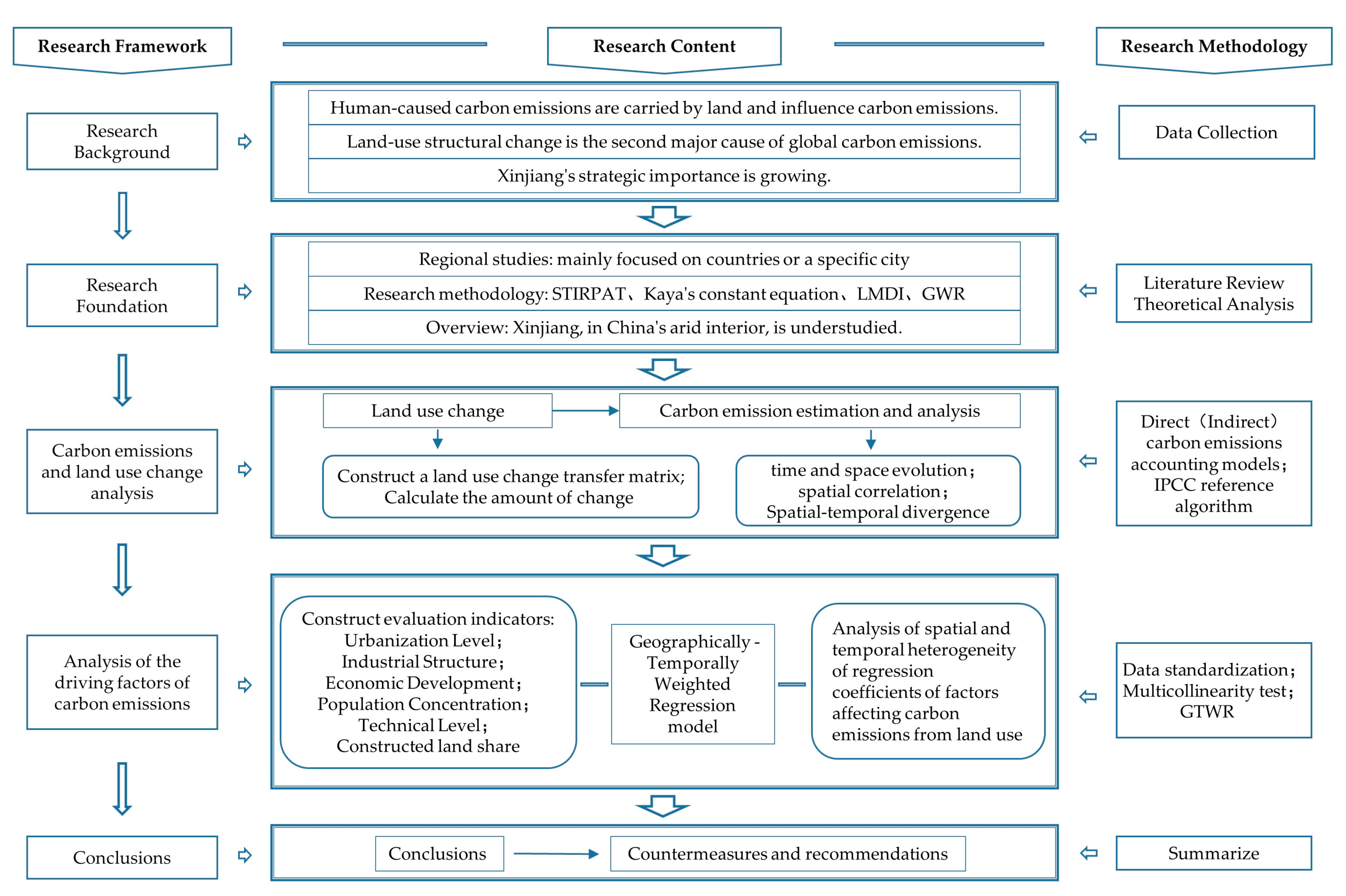
2. Materials and Methods
2.1. Data Sources
2.2. Research Methodology
2.2.1. Direct Carbon-Emission-Accounting Models
2.2.2. Indirect Carbon-Emission-Accounting Models
2.2.3. Indicator Dimensionless Processing
2.2.4. Geographically and Temporally Weighted Regression Model (GTWR)
3. Results
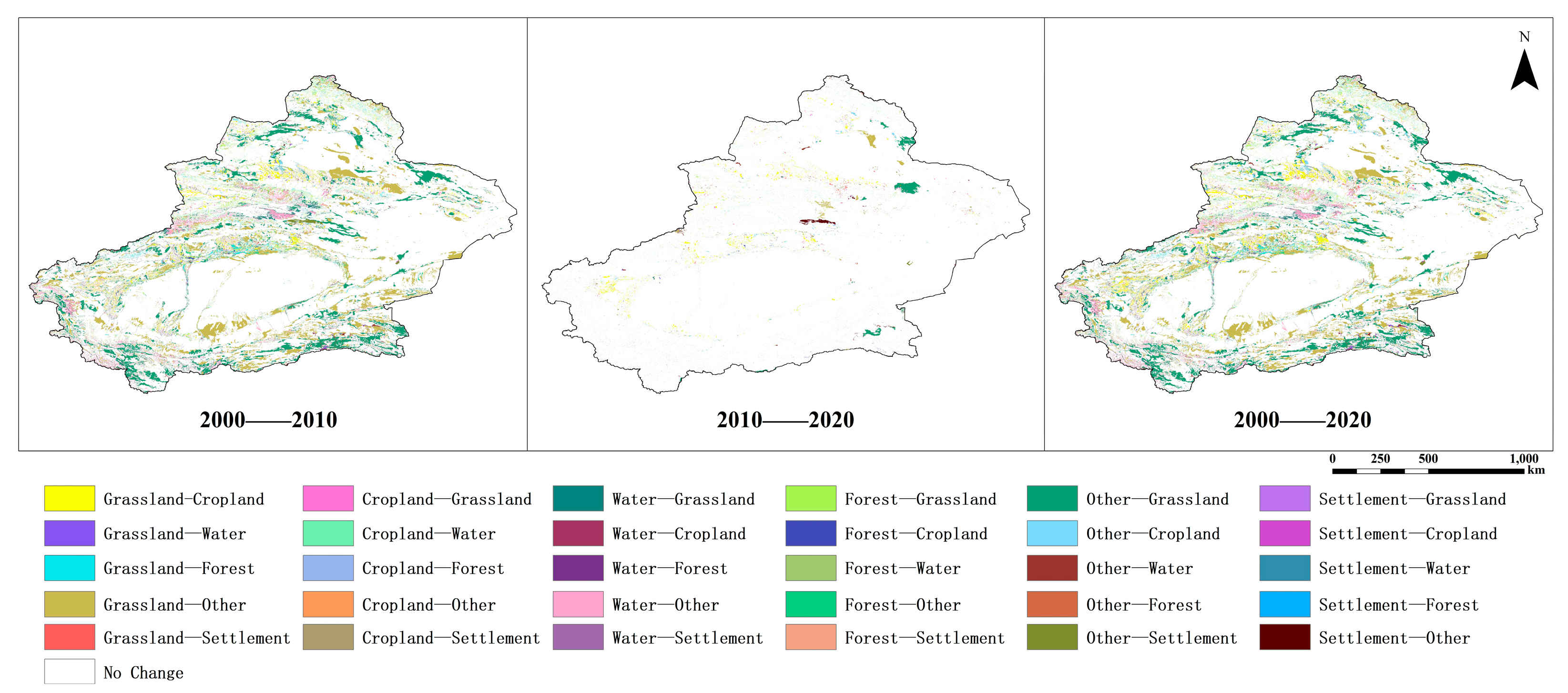
3.1. Spatio-Temporal Dynamic Analysis of Land Use Change in Xinjiang from 2000 to 2020
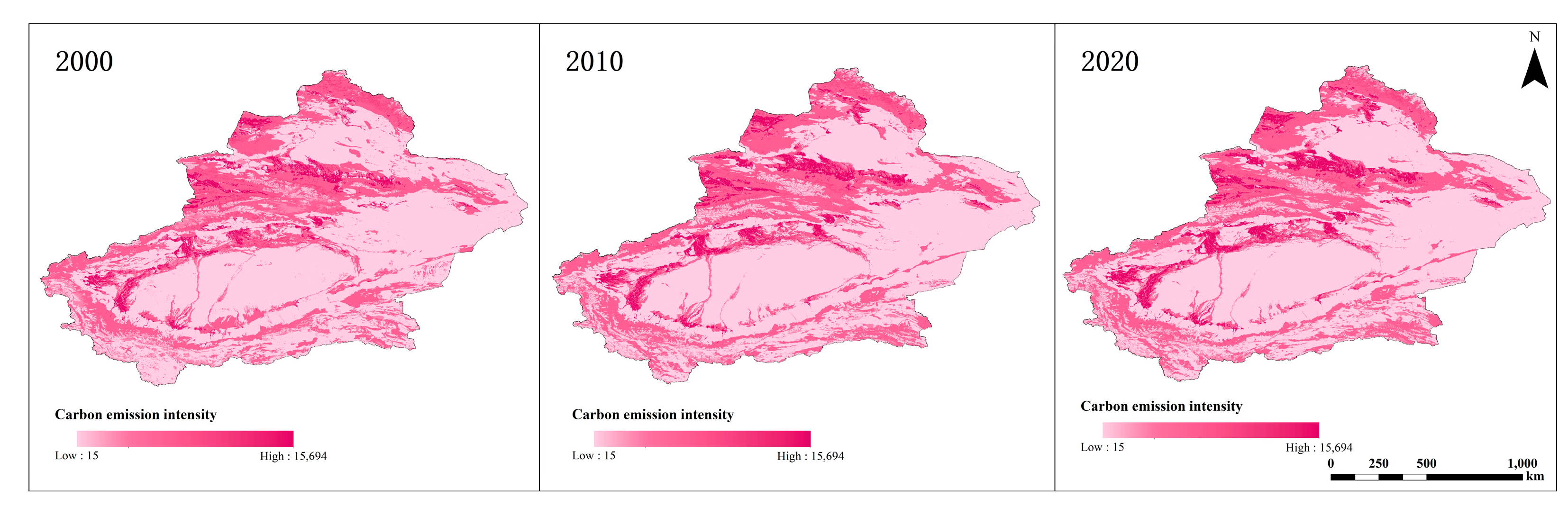
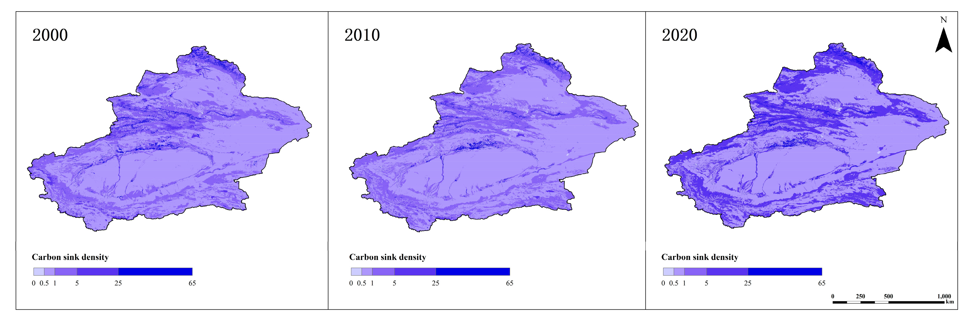
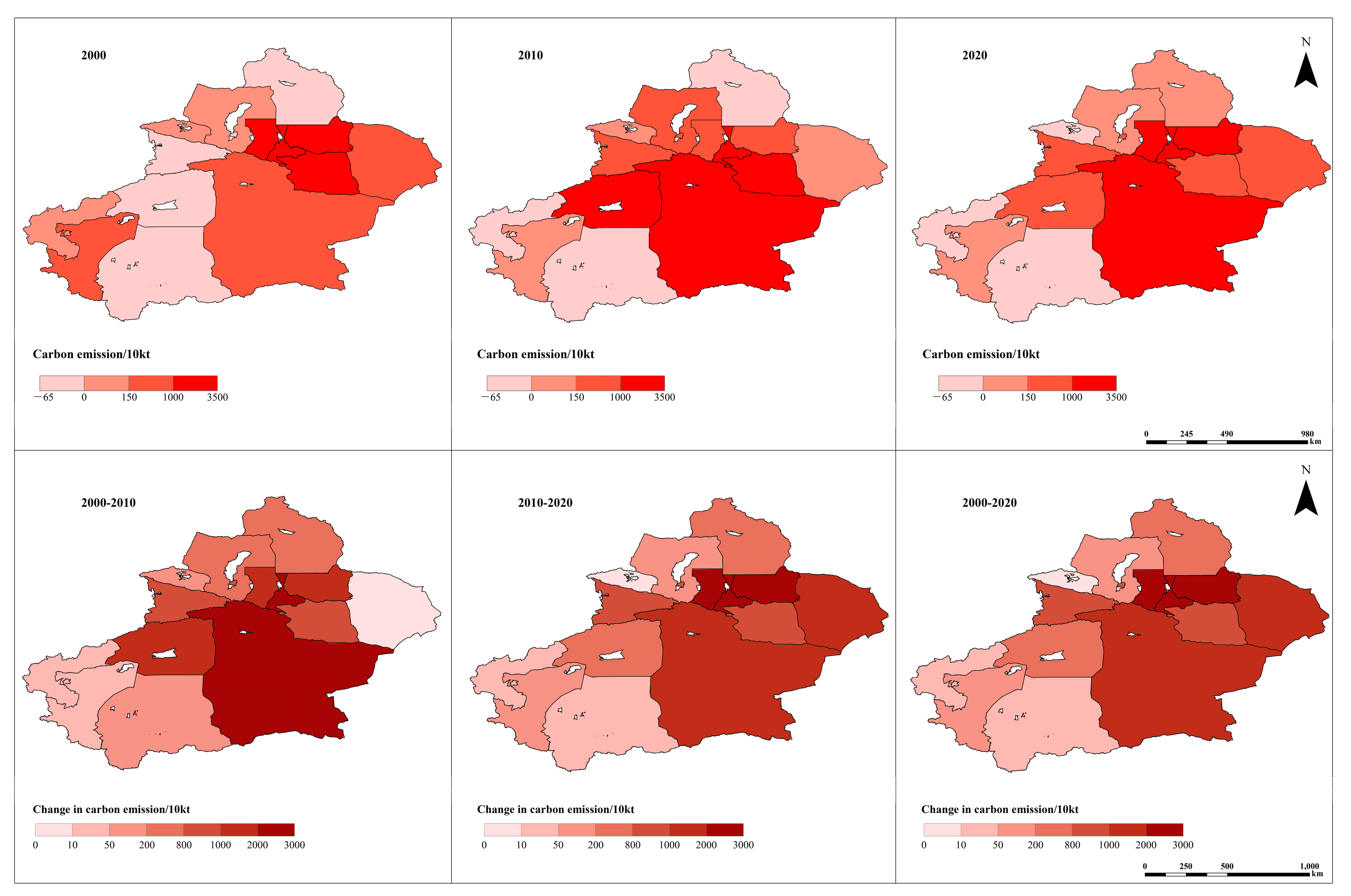
3.2. Analysis of Carbon Emissions from Land Use in Xinjiang from 2000 to 2020
3.3. Analysis of Carbon Emission Drivers
3.3.1. Data Testing
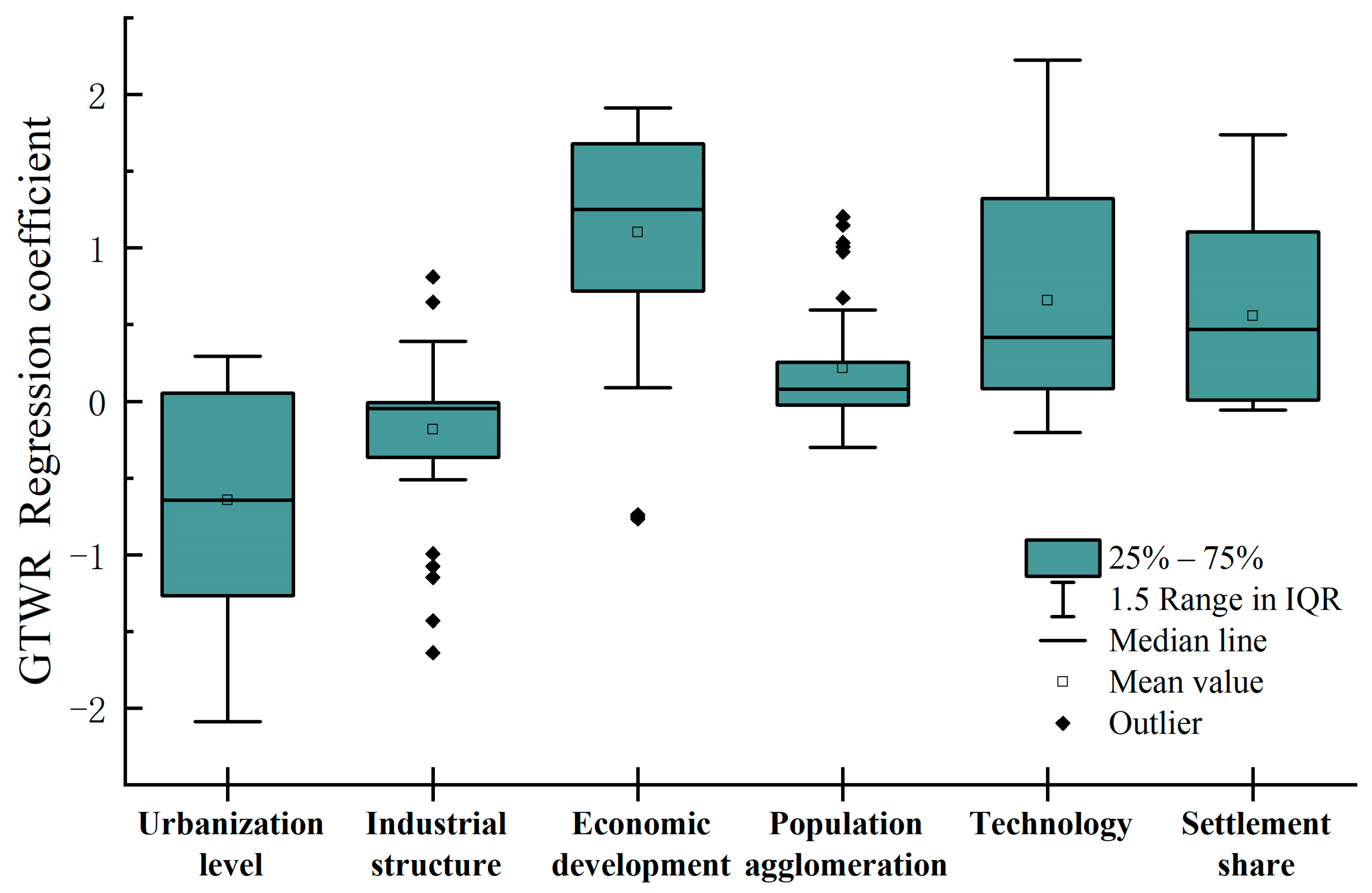
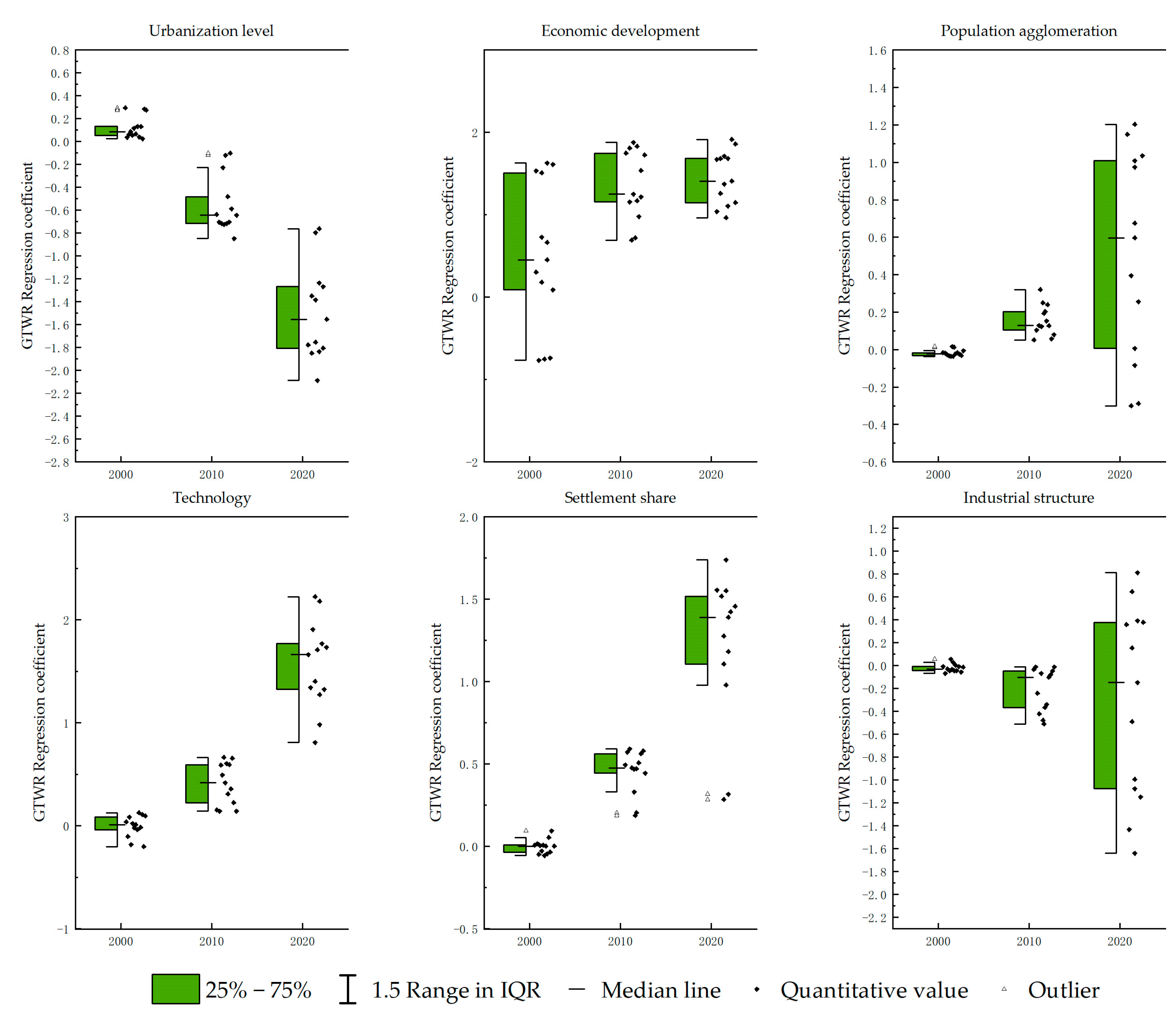
3.3.2. Analysis of Temporal Heterogeneity of Regression Coefficients of Factors Affecting Carbon Emissions from Land Use
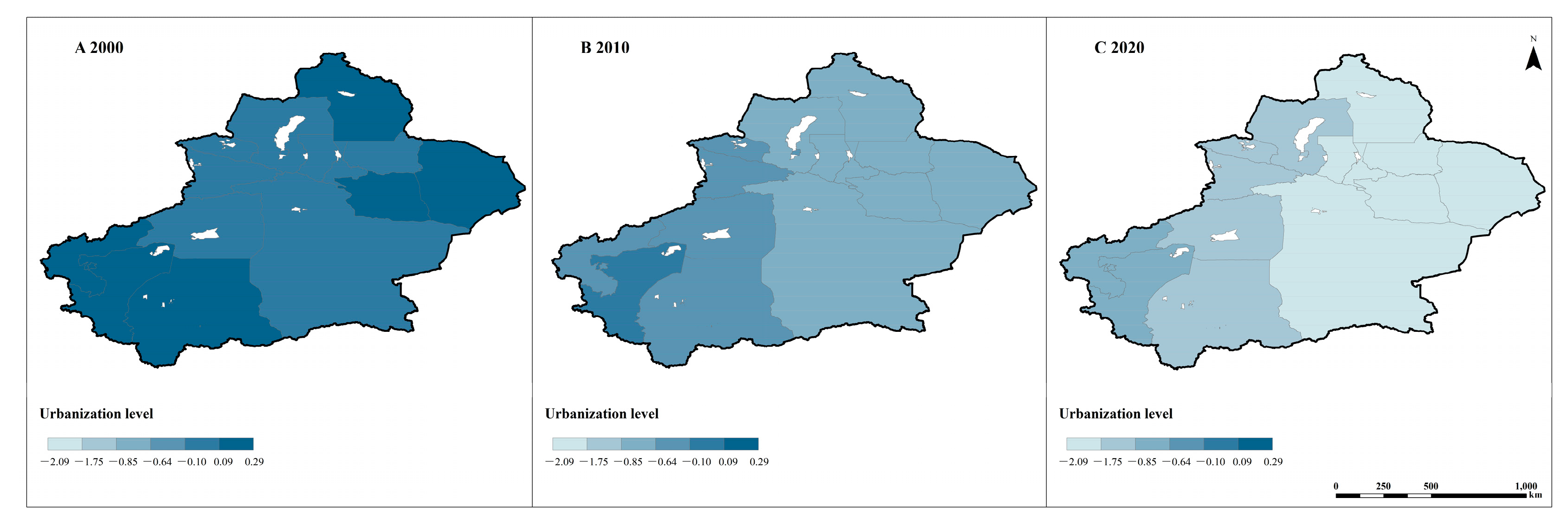
3.3.3. Analysis of Spatial Heterogeneity of Regression Coefficients of Factors Affecting Carbon Emissions from Land Use
- Urbanization level
- 2.
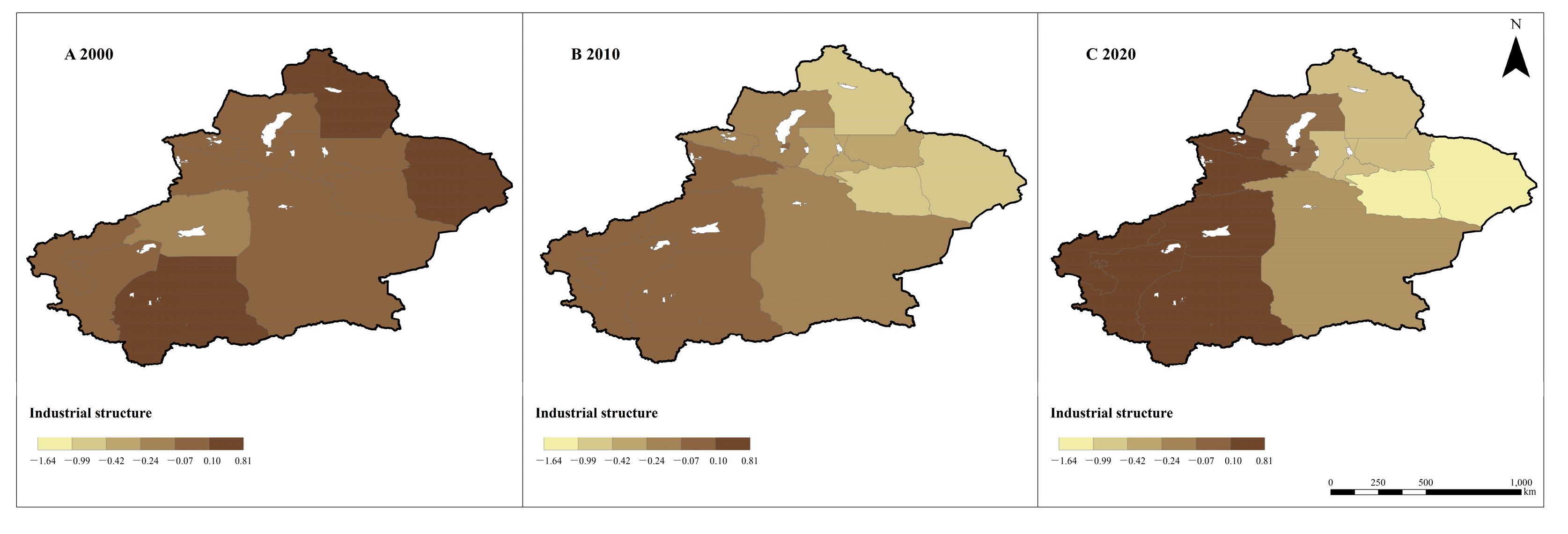
- Industrial structure
- 3.
- Economic development level
- 4.
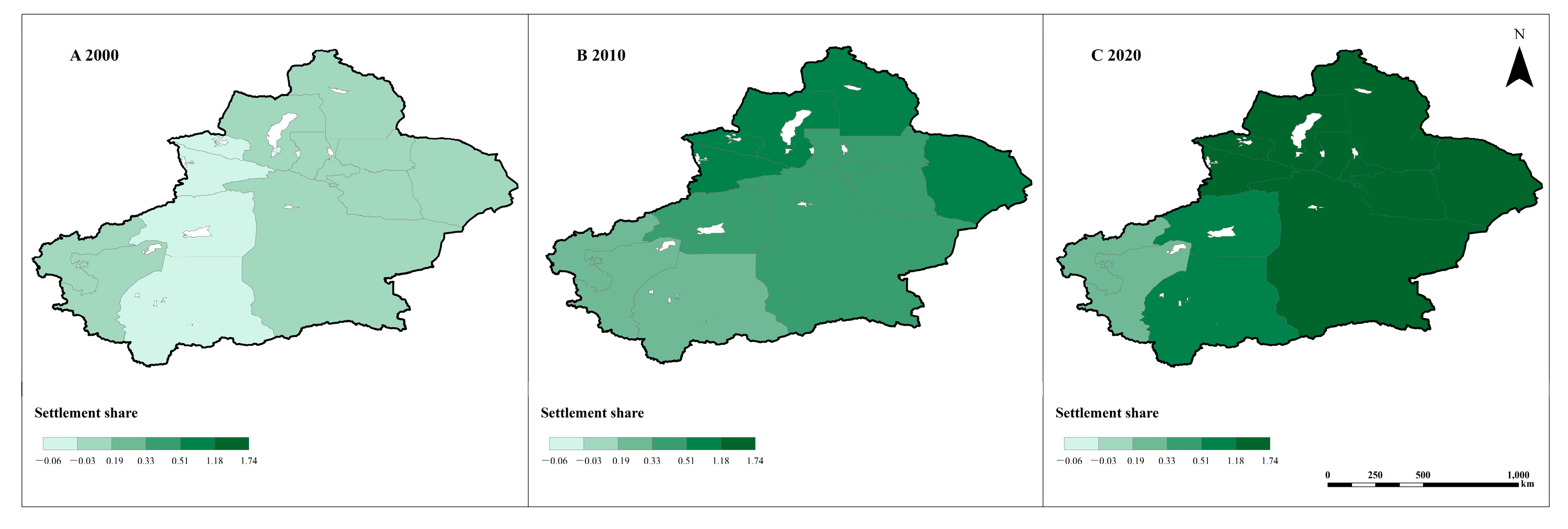
- Population agglomeration
- 5.
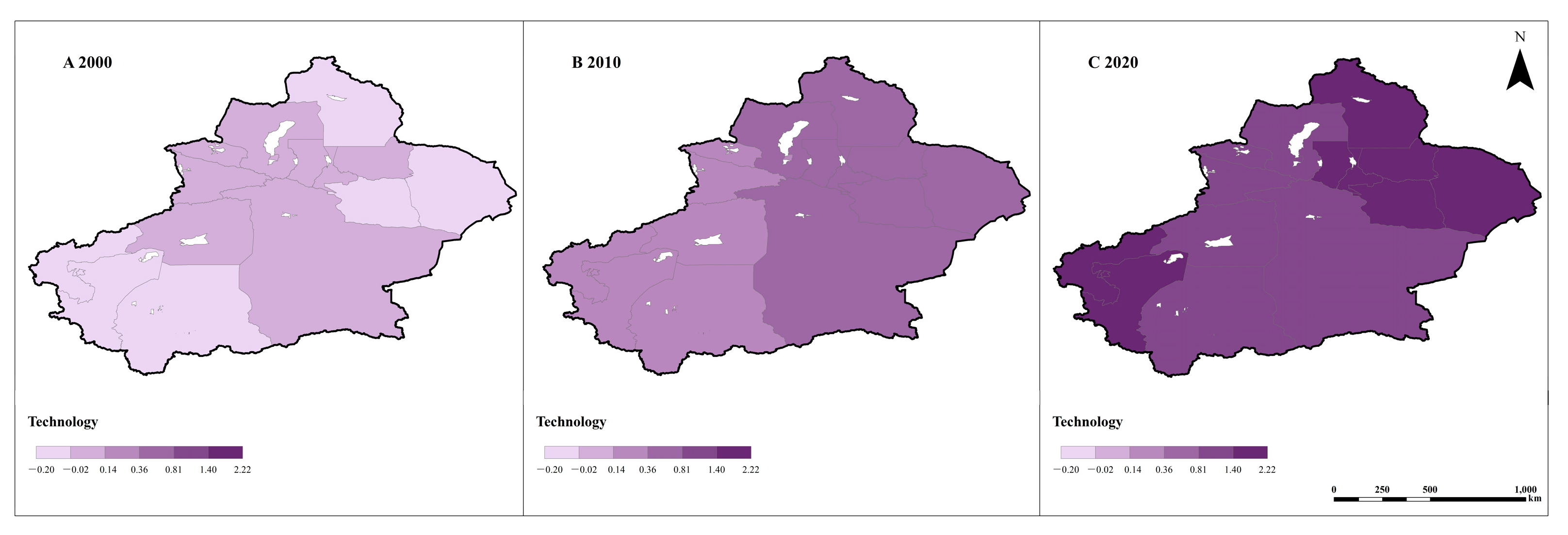
- Technology level
- 6.
- Proportion of construction land
4. Discussion
4.1. Study of Variations in Carbon Emissions Resulting from Land Use
4.2. Variability in Factors Affecting Carbon Emissions from Land Use over Space and Time
5. Conclusions
Author Contributions
Funding
Institutional Review Board Statement
Informed Consent Statement
Data Availability Statement
Acknowledgments
Conflicts of Interest
References
- IPCC. Climate Change 2021: The Physical Science Basis, Intergovernmental Panel on Climate Change; IPCC: Geneva, Switzerland, 2021. [Google Scholar]
- Sun, J.L. Evaluation of spatial agglomeration effects of urban carbon emissions based on spatial lag regression. Fresenius Environ. Bull. 2020, 29, 9805–9812. [Google Scholar]
- Yu, A.; Lin, X.; Zhang, Y.; Jiang, X.; Peng, L. Analysis of driving factors and allocation of carbon emission allowance in China. Sci. Total Environ. 2019, 673, 74–82. [Google Scholar] [CrossRef] [PubMed]
- Zhao, R.Q.; Liu, Y.; Hao, S.L.; Ding, M.L. Research on the Low-carbon Land Use Pattern. Res. Soil Water Conserv. 2010, 14, 190–194. [Google Scholar]
- Koch, G.W.; Mooney, H.A. Response of terrestrial ecosystems to elevated CO2: A synthesis and summary. In Carbon Dioxide and Terrestrial Ecosystems; Academic Press: San Diego, CA, USA, 1996; pp. 236–240. [Google Scholar]
- Houghton, R.A. Revised estimates of the annual net flux of carbon to the atmosphere from changes in land use and land management 1850–2000. Tellus B Chem. Phys. Meteorol. 2003, 55, 378–390. [Google Scholar]
- Zhou, T.; Shi, P. Indirect Impacts of Land Use Change on Soil Organic Carbon Change in China. Adv. Earth Sci. 2006, 21, 138–143. [Google Scholar]
- Qu Futian, L.; Na, F.S. Effects of land use change on carbon emissions. China Popul. Resour. Environ. 2011, 21, 76–83. [Google Scholar]
- Zuoji, D. The territorial planning under the concept of low-carbon. Urban Stud. 2010, 17, 1–5. [Google Scholar]
- Wu, J.G.; Zhai, P.M.; Wu, Y.T. New understanding on the land-based response options to climate change. Clim. Chang. Res. 2020, 16, 50–69. [Google Scholar]
- Zhao, X.C.; Zhu, X.; Zhou, Y.Y. Effects of land uses on carbon emissions and their spatial-temporal patterns in Hunan Province. Acta Sci. Circumstant. 2013, 33, 941–949. [Google Scholar]
- Garofalo, D.F.T.; Novaes, R.M.L.; Pazianotto, R.A.; Maciel, V.G.; Brandão, M.; Shimbo, J.Z.; Folegatti-Matsuura, M.I. Land-use change CO2 emissions associated with agricultural products at municipal level in Brazil. J. Clean. Prod. 2022, 364, 132549. [Google Scholar] [CrossRef]
- Houghton, R.A.; Hackler, J.L. Sources and sinks of carbon from land-use change in China. Glob. Biogeochem. Cycles 2003, 17, 1034. [Google Scholar] [CrossRef]
- Shuai, C.; Shen, L.; Jiao, L.; Wu, Y.; Tan, Y. Identifying key impact factors on carbon emission: Evidences from panel and time-series data of 125 countries from 1990 to 2011. Appl. Energy 2017, 187, 310–325. [Google Scholar] [CrossRef]
- Luo, H.; Gao, X.; Liu, Z.; Liu, W.; Li, Y.; Meng, X.; Yang, X.; Yan, J.; Sun, L. Real-time Characterization Model of Carbon Emissions Based on Land-use Status: A Case Study of Xi’an City, China. J. Clean. Prod. 2024, 434, 140069. [Google Scholar] [CrossRef]
- Zhang, M.; Lai, L.; Huang, X.J.; Chuai, X.W.; Tan, J.Z. The carbon emission intensity of land use conversion in different regions of China. Resour. Sci. 2013, 35, 792–799. [Google Scholar]
- Gingrich, S.; Kušková, P.; Steinberger, J.K. Long-term changes in CO2 emissions in Austria and Czechoslovakia—Identifying the drivers of environmental pressures. Energy Policy 2011, 39, 535–543. [Google Scholar] [CrossRef] [PubMed]
- Kang, T.; Wang, H.; He, Z.; Liu, Z.; Ren, Y.; Zhao, P. The effects of urban land use on energy-related CO2 emissions in China. Sci. Total Environ. 2023, 870, 161873. [Google Scholar] [CrossRef]
- Wu, Y.Z.; Ma, X.T.; Wu, K.; Huang, C.; Dai, H.C. Impact of Economic Growth and Structural Change on Carbon and Air Pollutant Emissions in Asian Countries: Analysis on Driving Force Based on KAYA, LMDI, and SDA Decomposition Method. Ecol. Econ. 2023, 39, 191–205. [Google Scholar]
- Ma, J.H.; Sun, Y.; Guo, Z.P.; He, Y.; Fan, M.Y. Research on Heterogeneity of the Impact of Influencing Factors on Carbon Emission in Hebei Province Based on GTWR Model. Ecol. Econ. 2023, 39, 23–29+49. [Google Scholar]
- Han, F.; Gao, F.; He, B.; Cao, Y.; Liu, K. Coupling coordination degree of carbon emissions in production, living and ecology space and influencing factors in the Aksu River Basin. Environ. Sci 2024. [Google Scholar] [CrossRef]
- Xing, Q. Research on the Relationship between Economic Development and Carbon Emissions Northwest Territory—Based on Panel Data Analysis. Master’s Thesis, Lanzhou Business School, Lanzhou, China, 2014. [Google Scholar]
- ICS:07.040; Current Land Use Classification. Standardization Administration of China (SAC): Beijing, China, 2017.
- Chen, P.; Wang, X.; Wang, L. Countermeasures for Carbon Balance and Sink Enhancement in China’s Terrestrial Ecosystems; Science Press: Beijing, China, 2008; pp. 108–121. [Google Scholar]
- Niu, Y.W.; Zhao, X.C.; Hu, Y.J. Spatial variation of carbon emissions from county land use in Chang-Zhu-Tan area based on NPP-VIIRS night light. Acta Sci. Circumstant. 2021, 41, 3847–3856. [Google Scholar]
- Xu, Y.; Guo, N.; Ru, K.L.; Fan, S.L. Characteristics and optimization strategies of territorial space zone in Fujian Province, China based on carbon neutrality. Chin. J. Appl. Ecol. 2022, 33, 500–508. [Google Scholar]
- Sun, H.; Liang, H.; Chang, X.; Cui, Q.; Tao, Y. Land use patterns on carbon emission and spatial association in China. Econ. Geogr. 2015, 35, 154–162. [Google Scholar]
- Li, L. Carbon Emission Effect of Land Use in China. Ph.D. Thesis, Nanjing University, Nanjing, China, 2010. [Google Scholar]
- Sun, S. Study on the Impact of Land Use Change on Carbon Emission and Counter Measures in Harbin. Master’s Thesis, Harbin Normal University, Harbin, China, 2020. [Google Scholar]
- Deng, L.; Li, H. Spatial and Temporal Evolution of Land Use Carbon Emissions and Analysis of Driving Factors in Wuhan Metropolitan Area. Res. Soil Water Conserv. 2024, 31, 345–353. [Google Scholar]
- Zhang, J.F.; Zhang, A.L.; Dong, J. Wuhan city circle effect of land use and carbon emissions factors decomposition. Res. Land Resour. Util. Ecol. Civiliz. Constr. China 2014, 23, 595–602. [Google Scholar]
- Li, M. Research on the Impact of Urban Development on Carbon Emissions in the Yellow River Basin under the Background of “Double Carbon” Policy. Ph.D. Thesis, Shandong Normal University, Jinan, China, 2023. [Google Scholar]
- Huang, B.; Wu, B.; Barry, M. Geographically and temporally weighted regression for modeling spatio-temporal variation in house prices. Int. J. Geogr. Inf. Sci. 2010, 24, 383–401. [Google Scholar] [CrossRef]


| Land Use Types | Carbon Emission Factor tC/(hm2-a) | References |
|---|---|---|
| cropland | 0.007 | Chen Panqin, Wang Xiaoke et al. [24] |
| forest | 0.644 | Niu Yawen, Zhao Xianchao et al. [25] |
| grassland | −0.021 | Xu Ying, Guo Nan et al. [26] |
| water | −0.253 | Sun He, Liang Hongmei et al. [27] |
| unutilized land | −0.005 | Lai Li [28]; Sun Shuangmei [29] |
| Type of Energy | Conversion Factor for Standard Coal kgce/kg | Carbon Emission Factor t/tce | Type of Energy | Conversion Factor for Standard Coal kgce/kg | Carbon Emission Factor t/tce |
|---|---|---|---|---|---|
| raw coal | 0.714 | 0.756 | gasoline | 1.471 | 0.571 |
| refined coal | 0.900 | 0.756 | diesel fuel | 1.457 | 0.592 |
| other coal washing | 0.285 | 0.216 | fuel oil | 1.429 | 0.619 |
| coke | 0.971 | 0.855 | liquefied petroleum gas | 1.714 | 0.504 |
| coke oven gas | 0.571 | 0.355 | refinery dry gas | 1.571 | 0.460 |
| blast furnace gas | 0.129 | 0.355 | other petroleum products | 1.400 | 0.586 |
| petroleum | 1.330 | 0.448 | thermodynamic | 0.034 | 0.670 |
| crude oil | 1.429 | 0.586 | electrical power | 0.345 | 0.272 |
| diesel | 1.471 | 0.554 | other fuels | 0.645 | 0.756 |
| Year | Sports Event | Cropland | Forest Land | Grassland | Waters | Constructed Land | Unutilized Land |
|---|---|---|---|---|---|---|---|
| 2000~2010 | rate of change | 35.83 | −25.94 | 1.77 | −35.53 | 83.70 | −0.48 |
| dynamic degree | 3.58 | −2.59 | 0.18 | −3.55 | 8.37 | −0.05 | |
| 2010~2020 | rate of change | 11.62 | −2.56 | −0.61 | 3.45 | 12.66 | −0.79 |
| dynamic degree | 1.16 | −0.26 | −0.06 | 0.35 | 1.27 | −0.08 | |
| 2000~2020 | rate of change | 51.62 | −27.83 | 1.15 | −33.30 | 106.96 | −1.27 |
| dynamic degree | 2.58 | −1.39 | 0.06 | −1.67 | 5.35 | −0.06 |
| Particular Year | 2000 | 2010 | 2020 | |
|---|---|---|---|---|
| Carbon Sinks | cropland | −4.15 | −5.64 | −5.64 |
| forest | −245.01 | −181.46 | −176.82 | |
| grassland | −100.92 | −101.79 | −101.17 | |
| waters | −130.94 | −84.41 | −87.34 | |
| unutilized land | −50.01 | −49.76 | −49.37 | |
| carbon absorption total amount | −530.13 | −423.07 | −420.33 | |
| Carbon Sources | cropland | 88.26 | 116.61 | 139.23 |
| constructed land | 1195.27 | 3224.23 | 14,149.60 | |
| carbon emission total amount | 1283.53 | 3340.84 | 14,288.84 | |
| Net Carbon Emission | 753.40 | 2917.77 | 13,868.51 | |
| Indicator Name | Hidden Meaning | VIF Value |
|---|---|---|
| Urbanization Level (of a city) | urban resident population/total population | 3.757 |
| Industrial Structure | secondary sector output/gross output | 1.648 |
| Level of Economic Development | GDP per capita | 2.171 |
| Degree of Population Concentration | permanent population per unit area | 1.801 |
| Technical Level | energy consumption per unit of GDP | 1.567 |
| Percentage of Constructed land | proportion of constructed land to urban area | 2.870 |
| Model | Bandwidth | Residual Squares | Sigma | AICc | R2 | R2 Adjusted |
|---|---|---|---|---|---|---|
| GTWR | 0.196 | 0.607 | 0.125 | 238.549 | 0.984 | 0.981 |
Disclaimer/Publisher’s Note: The statements, opinions and data contained in all publications are solely those of the individual author(s) and contributor(s) and not of MDPI and/or the editor(s). MDPI and/or the editor(s) disclaim responsibility for any injury to people or property resulting from any ideas, methods, instructions or products referred to in the content. |
© 2024 by the authors. Licensee MDPI, Basel, Switzerland. This article is an open access article distributed under the terms and conditions of the Creative Commons Attribution (CC BY) license (https://creativecommons.org/licenses/by/4.0/).
Share and Cite
Yang, J.; Li, K.; Liu, Y.; Zhang, Y. Time-Space Evolution and Drivers of CO2 Emissions from Land Utilization in Xinjiang from 2000 to 2020. Sustainability 2024, 16, 2929. https://doi.org/10.3390/su16072929
Yang J, Li K, Liu Y, Zhang Y. Time-Space Evolution and Drivers of CO2 Emissions from Land Utilization in Xinjiang from 2000 to 2020. Sustainability. 2024; 16(7):2929. https://doi.org/10.3390/su16072929
Chicago/Turabian StyleYang, Jingye, Kenan Li, Yongqiang Liu, and Yongfu Zhang. 2024. "Time-Space Evolution and Drivers of CO2 Emissions from Land Utilization in Xinjiang from 2000 to 2020" Sustainability 16, no. 7: 2929. https://doi.org/10.3390/su16072929
APA StyleYang, J., Li, K., Liu, Y., & Zhang, Y. (2024). Time-Space Evolution and Drivers of CO2 Emissions from Land Utilization in Xinjiang from 2000 to 2020. Sustainability, 16(7), 2929. https://doi.org/10.3390/su16072929