Enhancing Wind Turbine Blade Preventive Maintenance Procedure through Computational Fluid Dynamics-Based Prediction of Wall Shear Stress

Abstract

Wind turbine blades are essential parts of wind energy systems and are frequently exposed to harsh environmental elements, such as strong winds, turbulence, and corrosive atmospheric elements. Over time, these circumstances may result in serious harm to blades, such as delamination and erosion, which may negatively affect the wind turbine’s functionality and durability. Accurate prediction of various types of damage is crucial to improve the toughness and lifespan of wind turbine blades and to maximize the overall effectiveness of wind energy systems. This article presents a novel computational fluid dynamics (CFDs)-based method for analyzing the distribution of wall shear stress on turbine blades, aimed at publicizing the yearly maintenance procedure. The investigation results from the CFDs, when compared with the current situation in a wind turbine farm in Thailand, confirmed that our wall shear stress modeling accurately predicted wind turbine damage. A maximum wall shear stress level higher than 5.00 Pa in the case of PA 90°, incoming air velocity 10.00 m/s, and 15 rpm was the main contribution to presenting the erosion and delamination from current drone inspection in wind turbine farms. In conclusion, these findings demonstrated the potential of using CFDs to predict wind turbine blade delamination and erosion, thereby significantly contributing to the development of specific and accurate yearly preventive maintenance. The proposed CFDs-based approach should serve as a sustainability tool for local human development, benefiting wind turbine engineers and operating technicians by providing them with a deeper understanding of the local flow conditions and wall shear stress distribution along wind turbine blades. This enables them to make informed decisions regarding blade design and maintenance.

1. Introduction

The issue of wind turbine farms is regular maintenance to ensure efficiency during operation. A proper yearly maintenance schedule will reduce the gap in power generation performance. However, for a developed country that cannot produce its commercial wind turbines, such as Thailand, it may be difficult to establish efficient maintenance planning, even if the manufacturer’s instructions are followed, considering the specific geographical conditions, blade shape complexity, and wind behavior. Human development is pivotal for the sustainability of specific knowledge for wind turbine farms, aiming to reduce reliance on external knowledge that cannot be applied locally. Hence, this article is initiated under this condition, building on previous research as follows. The exploration of a rotating turbine in terms of experimental tests and numerical simulations is challenging. Information from energy extraction in wind turbines is imperative to improve the operation and lifetime of wind turbines [1,2]. Our literature review indicated, starting from 2016, that CFDs have been used to simulate the aerodynamics of a full-scale horizontal axis wind turbine, providing valuable information on the flow conditions and aerodynamic performance [3]. The investigation showed that dimensional scaling significantly impacts wind turbine performance. It is essential to consider its effects when designing wind turbine blades [4]. The CFD results showed the angle of attack significantly impacts the wind turbine’s aerodynamic performance, affecting the lift and drag forces [5]. One study analyzed a variable twist blade for horizontal axis wind turbines based on numerical simulation with Reynolds-averaged Navier–Stokes equations using the k-ω shear stress transport turbulence model coupled with one-way fluid–structure interaction [6]. Another simulation study using the force distribution information showed significant fluctuations on the blades [7]. The characteristics and modeling of the wake for multiple aligned turbines based on numerical simulation indicated that spacing significantly affects the superposition model’s performance [8]. The prediction results from mean velocity and turbulent kinetic energy showed that significant improvement can be achieved compared to baseline cases [9]. The pitching motion effects along with high reduced frequencies and a deep dynamic stall condition were investigated using a large eddy simulation approach. The prediction results of the lift, drag, and moment coefficients were in good agreement with the available experimental data and other numerical results in the literature [10]. The effects of blade surface roughness on wind turbine performance were tested using three rotors that were designed using the NACA4415, S801, and S810 airfoils. The numerical evaluation confirmed that the roughened blades had performance deterioration within the range 2.9–8.6% for a torque-based control strategy [11]. MATLAB Simulink was used to examine the functional modeling of weather vane behavior, leading to the estimation of yawing error and evaluation of the corresponding power reduction [12].

For an understanding of the experiment, a more concentrated and super-large-scale particle image velocimetry (SLS-PIV) of a utility-scale wind turbine has been used to provide important insights into the flow conditions around the turbine [13]. Additional techniques measured the incoming flow parameters in real time and with high accuracy, allowing for a detailed understanding of the flow conditions at the blade scale. This realistic information can inform maintenance and repair strategies, ensuring the wind turbine operates optimally for its lifespan [14]. The interaction between a small stand-alone wind turbine nacelle and a tower has been studied using field measurements, with the results indicating distortion with low power spectrum frequencies [15]. The effect of boundary proximity and blockage has been examined experimentally, with the results showing that the benefits of the blockage and speed in power extraction were offset by the wake prolongation [16]. A wind tunnel study was adapted to compare the turbulence in the wakes of an actuator disc and a model wind turbine using higher-order statistics. The researchers concluded that the turbine generated specific turbulence characteristics that dominated the ambient turbulence and had strong features of isotropic turbulence [17]. The diagonal inflow has been measured using ultrasonic anemometers for velocity, a three-cup type anemometer, and the wind vane, respectively. The measurement results indicated that the maximum power coefficients corresponded to the tip ratio and pitch angle [18]. Next, the relationship between the incoming flow field and the turbine power fluctuations was explored using the particle image velocimetry technique. It demonstrates that all incoming aerodynamic characteristics are critical for wind turbine performance [19]. Hence, from the literature review, most research papers identified factors such as confirming local incoming conditions, wind turbine geometry, and the terrain that affected turbine operation and performance. All these factors were also recognized as sources of failure and damage to the wind turbine [20,21].

To date, anti-erosion techniques using carbon nanotubes and graphene nano-additives have shown significant improvement [22]. The possibility of developing new anti-erosion coatings for wind turbine blade surface protection based on nanoengineered polymers is explored. It has been demonstrated that graphene and hybrid (graphene/silica) reinforced polymer coatings can provide better erosion protection with lifetimes up to 13 times longer than non-reinforced polyurethanes [23]. Notably, the leading edge of the wind turbine is the most erosion-prone area as the edge is subjected to high pressure and shear force, which induce erosion, corrosion, and layer delamination [24,25].

The wind turbine is an extremely complex design, with several airfoil sections and twisted blades that make repair difficult. Furthermore, generating a 3D simulation model is difficult without 3D laser scanning or drone inspection. For these reasons, wind turbine engineers need to minimize the risk of damage as much as possible. One efficient preventive maintenance measure is crucial, despite the advanced nanomaterial technology. Wall shear stress is a critical factor in causing damage [26,27], as it can lead to corrosion, delamination, and erosion. The distribution of wall shear stress along the blade surface is an important parameter to consider when predicting damage and developing strategies to enhance blade durability. Previous literature reviews primarily explain the numerical technique, sources of damage, and prevention of damage using nano-material coatings, but they still lack information regarding the force acting on the wall of the turbine blade related to the incoming and operational conditions [5,20,21,22,26,27]. In the current study, a computational fluid dynamics (CFDs) simulation is employed to analyze the wall shear stress distribution on a full-scale horizontal axis wind turbine blade. The simulation considers various operational scenarios, including different local wind speeds, realistic pitch angles, and transition turbulence models. The simulation findings are then compared to experimental data from Thailand’s Lamthakhong Wind Turbine Farm located at Nakhon Ratchasima Province Northeast Thailand, which is operated by the Electricity Generating Authority of Thailand (EGAT), to ensure the correctness and reliability of the CFDs methodology. The gap between standardization and best practice protocols for preventive maintenance may be improved through computational fluid dynamics-based prediction of wall shear stress. The end result will be a recommendation to the wind turbine maintenance staff to evaluate the technique using actual data. Nonetheless, this maintenance schedule has been extended to include another wind farm site, as well as EGAT’s internal human development strategy for sustainability.

2. Wind Turbine Geometry

In this study, the blade of a wind turbine is quite intricate, integrating various types of high-fidelity designed airfoils from the manufacturer. The FARO Laser Scanner Focus3D was utilized to perform high-precision laser scanning of a wind turbine. The resolution of the scanning process was determined by the point cloud density, which was specified as 250,000 points per second, with an accuracy of ±2 mm. The resulting point cloud from 15 scanning locations was sufficiently dense to generate a highly accurate 3D model of the wind turbine, as shown in Figure 1. Several parameters were compared to those provided by wind turbine engineers to ensure that the 3D model of the wind turbine generated from the laser scanning process accurately represented the realistic structure. The results showed that the generated geometry agreed with the original engineering drawings. The detailed drawings of the wind turbine provided by the manufacturer are considered intellectual property, and thus cannot be shown in more detail in this study. However, the high-precision 3D laser scanning technology used in this study has been widely utilized in various fields and is an effective tool for generating accurate 3D models of complex structures [28,29]. The next section will discuss the mathematical model for fluid dynamics analysis, as well as data accuracy justification, based on statistical analysis and wall shear stress interpretation.

3. Mathematical Formulation

From the previous literature review, many research papers suggested that the SST k-ω turbulence model provides more accurate predictions for near-wall aerodynamic variables. In addition, some options have been implemented to increase the wall accuracy for the wall shear stress calculation. The first one included in the current study is the turbulence transition on the wall. This option remains open when the low wind speed and marginalization between laminar and turbulence, aligning with the local wind speed, are marginally low in some seasons. Therefore, it is appropriate to include this option in the study, particularly considering the specific terrain of the Lamthakhong Wind Farm. The general governing and transport equation can be described as

$$\nabla \cdot \left(\rho \overrightarrow{U}\right)=0$$

(1)

$$\nabla \cdot \left(\rho \overrightarrow{U}\overrightarrow{U}\right)=-\nabla P+\nabla \cdot \left[\left(\nabla \overrightarrow{U}+\nabla {\overrightarrow{U}}^T\right)-\frac{2}{3}\nabla \cdot \overrightarrow{U}I\right]$$

(2)

$$\frac{\partial }{\partial x_i}\left(\rho k{U}_i\right)=\frac{\partial }{\partial x_j}\left[\left(\mu +\frac{{\mu }_t}{{\sigma }_k}\right)\frac{\partial k}{\partial x_j}\right]+{\Phi }_k-{\Psi }_k$$

(3)

$$\frac{\partial }{\partial x_i}\left(\rho \omega U_i\right)=\frac{\partial }{\partial x_j}\left[\left(\mu +\frac{{\mu }_t}{{\sigma }_{\omega }}\right)\frac{\partial \omega }{\partial x_j}\right]+{\Phi }_{\omega }-{\Psi }_{\omega }+D_{\omega }$$

(4)

All the turbulence model constants in Equations (1)–(4) can be found in [30,31] where $\rho$ is the air density, $\overrightarrow{U}$ is the velocity vector, $P$ is the pressure, $k$ is the turbulence kinetic energy, ${\mu }_t$ is the turbulence viscosity, and $\omega$ is the specific dissipation rate. An important aspect in this investigation was the high levels of wall shear stress that can cause wear and damage to the blades. Consequently, managing wall shear stress is an important aspect of preventive maintenance to ensure that wind turbines are operating optimally. The equation representing this is

$${\tau }_w=\mu \frac{du}{dz}$$

(5)

where ${\tau }_w$ is the wall shear stress, the rate of change of velocity $u$ with respect to distance is the velocity gradient on the wall and $\mu$ is the dynamic viscosity. From Equation (5), the key contributing variable is velocity, which is related to the incoming air speed in this situation. We chose wall shear stress to predict wind turbine damage. Based on this assumption, it is not a direct variable to estimate flow-induced erosion and delamination directly, but it is an appropriate way to utilize the incoming wind speed from the WindSCADA system.

Transport Equations for Transition SST Model

Two additional transport equations, one for the intermittency factor and one for the momentum-thickness Reynolds number, defined for the transition onset criteria were coupled in the transition SST model. In addition, the empirical correlation from Langtry and Menter was developed to include standard bypass transitions and flows in low and freestream turbulence environments. The transport equation of the intermittency factor ($\gamma$) is rewritten as

$$\frac{\partial (\rho U_j\gamma )}{\partial x_j}={\Gamma }_{\gamma 1}-{{\rm E}}_{\gamma 1}+{\Gamma }_{\gamma 2}-{{\rm E}}_{\gamma 2}+\frac{\partial }{\partial x_j}\left[\left(\mu +\frac{{\mu }_t}{{\sigma }_{\gamma }}\right)\frac{\partial \gamma }{\partial x_j}\right]$$

(6)

The transition sources (${\Gamma }_{\gamma 1}$,$E_{\gamma 1}$) are defined as

$${\Gamma }_{\gamma 1}=C_{a1}{F}_{length}\rho S{\left[\gamma F_{onset}\right]}^{C_{\gamma 3}}$$

(7)

$$E_{\gamma 1}=C_{e1}{\Gamma }_{\gamma 1}\gamma$$

(8)

The strain rate magnitude is defined by $S$, while the term $F_{length}$ is an empirical correlation which determines the length of transition regions. The constant $C_{a1}$ is set to 2, while the constant $C_{e1}$ is close to 1. The source from destruction or relaminarization term (${\Gamma }_{\gamma 2}$, $E_{\gamma 2}$) is defined as

$${\Gamma }_{\gamma 2}=C_{a2}\rho \Omega \gamma F_{turb}$$

(9)

$$E_{\gamma 2}=C_{e2}{\Gamma }_{\gamma 2}\gamma$$

(10)

where $\Omega$ is the vorticity magnitude. The following functions control the transition onset:

$${\mathrm{Re}}_V=\frac{\rho y^{2}S}{\mu }$$

(11)

$${\mathrm{R}}_T=\frac{\rho k}{\mu \omega }$$

(12)

$${\mathrm{F}}_{onset1}=\frac{{\mathrm{Re}}_V}{2.193{\mathrm{Re}}_{\theta c}}$$

(13)

$$F_{onset2}=\min (\max (F_{onset1},F_{onset1}^4),2.0)$$

(14)

$$F_{onset3}=\max (1-{\left(\frac{R_T}{2.5}\right)}^3,0)$$

(15)

$$F_{onset}=\max (F_{onset2}-F_{onset3},0)$$

(16)

$$F_{turb}=e^{-{\left(\frac{R_T}{4}\right)}^4}$$

(17)

The term $y$ is the wall distance and ${\mathrm{Re}}_{\theta c}$ is the critical Reynolds number, which is a starting point where the intermittency factor begins to increase within the boundary layer upstream of the transition momentum thickness Reynolds number (${\widetilde{\mathrm{Re}}}_{\theta t}$). In particular, the correlations of $F_{length}$ and ${\mathrm{Re}}_{\theta c}$ are dependent on ${\widetilde{\mathrm{Re}}}_{\theta t}$. The constant terms for the intermittency factor equation are

$$C_{a1}=2;C_{e1}=1;C_{a2}=0.06;C_{e2}=50;C_{\gamma 3}=0.5;{\sigma }_{\gamma }=1.0$$

(18)

The transition momentum thickness Reynolds number $({\mathrm{Re}}_{\theta t})$ is included in the transport equation as

$$\frac{\partial \left(\rho U_j{\widetilde{\mathrm{Re}}}_{\theta t}\right)}{\partial x_j}={\Gamma }_{\theta t}+\frac{\partial }{\partial x_j}\left[2\left(\mu +{\mu }_t\right)\frac{\partial {\widetilde{\mathrm{Re}}}_{\theta t}}{\partial x_j}\right]$$

(19)

The source term is defined as

$${\Gamma }_{\theta t}=\frac{0.03{\left(\rho U\right)}^2}{500\mu }\left[{\mathrm{Re}}_{\theta t}-{\widetilde{\mathrm{Re}}}_{\theta t}\right]\left[1.0-F_{\theta t}\right]$$

(20)

$$F_{\theta t}=\min \left(\max \left(F_{wake}{e}^{{\left(-\frac{y}{\delta }\right)}^4}\right),1.0-{\left(\frac{\gamma -1/50}{1.0-1/50}\right)}^2,1.0\right)$$

(21)

$$\delta =\frac{375\Omega y{\widetilde{\mathrm{Re}}}_{\theta t}\mu }{\rho U^2}$$

(22)

$$F_{wake}=e^{-{\left(\frac{\rho \omega y^2}{\mu }\frac{1}{1E+5}\right)}^2}$$

(23)

In addition, the transition SST k-ω model contains a modification for separation-induced transition as defined by

$${\gamma }_{sep}=\min \left(2\max \left[\left(\frac{{\mathrm{Re}}_v}{3.235{\mathrm{Re}}_{\theta c}}\right)-1,0\right]e^{-{\left(\frac{R_T}{20}\right)}^4},2\right)F_{\theta t}$$

(24)

$${\gamma }_{eff}=\max (\gamma ,{\gamma }_{sep})$$

(25)

Hence, all relation equations and turbulence parameters of the transition SST k-ω are included in the transition model, which interact with the SST k-ω turbulence model by modification of the k-equation, as

$$\frac{\partial }{\partial x_i}\left(\rho k{u}_i\right)=\frac{\partial }{\partial x_j}\left(\left(\mu +{\sigma }_k{\mu }_t\right)\frac{\partial k}{\partial x_j}\right)+{\gamma }_{eff}\widetilde{G_k}-\min \left(\max \left({\gamma }_{eff},0.1\right),1.0\right)Y_k$$

(26)

$$\frac{\partial \left(\rho u_j\omega \right)}{\partial x_j}=\alpha \frac{P_k}{{\nu }_t}-D_{\omega }+C{d}_{\omega }+\frac{\partial }{\partial x_j}\left[\left(\mu +{\rho }_k{\mu }_t\right)\frac{\partial \omega }{\partial x_j}\right]$$

(27)

where $G_k$ and $Y_k$ are the original production and destruction terms, respectively, for the SST model. More detailed information of the above model formulation can be found in the literature [31]. To perform numerical results of the laminar and transitional boundary layers correctly, the normalized wall distance $\left(y^{+}\right)$ of the mesh must be close to one. If $y^{+}$ is greater than 5, then the location of the transition onset may move upstream, along with an increase in $y^{+}$. The mean flow, turbulence, and transition equations should use the bounded, second-order, upwind-based discretization to achieve solution convergence, as recommended by ANSYS Fluent.

Since the SST k-ω model is a hybrid model, the blending function $F_1$ has been used to control switching between the k-ω and k-ε models. The k-ω model is well suited near wall regions, while the result predictions from the k-ε models are good far away from the wall. Therefore, with near wall treatment for the SST k-ω model, the modified blending function $F_1$ is activated and is defined as

$${\mathrm{Re}}_y=\frac{\rho y\sqrt{k}}{\mu }$$

(28)

$$F_3=e^{-{\left(\frac{R_y}{120}\right)}^8}$$

(29)

$$F_1=\max (F_{1origin},F_3)$$

(30)

where $F_{1origin}$ is the original blending function from the SST k-ω turbulence model.

4. Solution Method

This section provides details of the numerical approach for the current model. Initially, boundary and initial conditions are proposed based on site measurements, while statistical tools are applied to interpret the prediction data. In addition, the grid independence study is reported and compared. We also validate the simulation results with available data to ensure that all numerical inputs are accurate. The numerical simulation settings for all cases are shown in

Table 1. ANSYS Fluent numerical setting.

Solution Controls	Methods
Pressure–Velocity Coupling	Coupled
Flux Type	Rhie-Chow
Pressure	2nd Order
Momentum	2nd Order Upwind
Turbulent Kinetic Energy	2nd Order Upwind
Specific Dissipation Rate	2nd Order Upwind
Intermittency	2nd Order Upwind
Momentum Thickness Re	2nd Order Upwind
Residual Monitors	Absolute Criteria 10−4
Flow Multigrid	F-Cycle
Turbulent Kinetic Energy Multigrid	F-Cycle
Specific Dissipation Rate Multigrid	F-Cycle
Intermittency Multigrid	F-Cycle
Momentum Thickness Re Multigrid	F-Cycle

.

4.1. Boundary Conditions and Initial Conditions

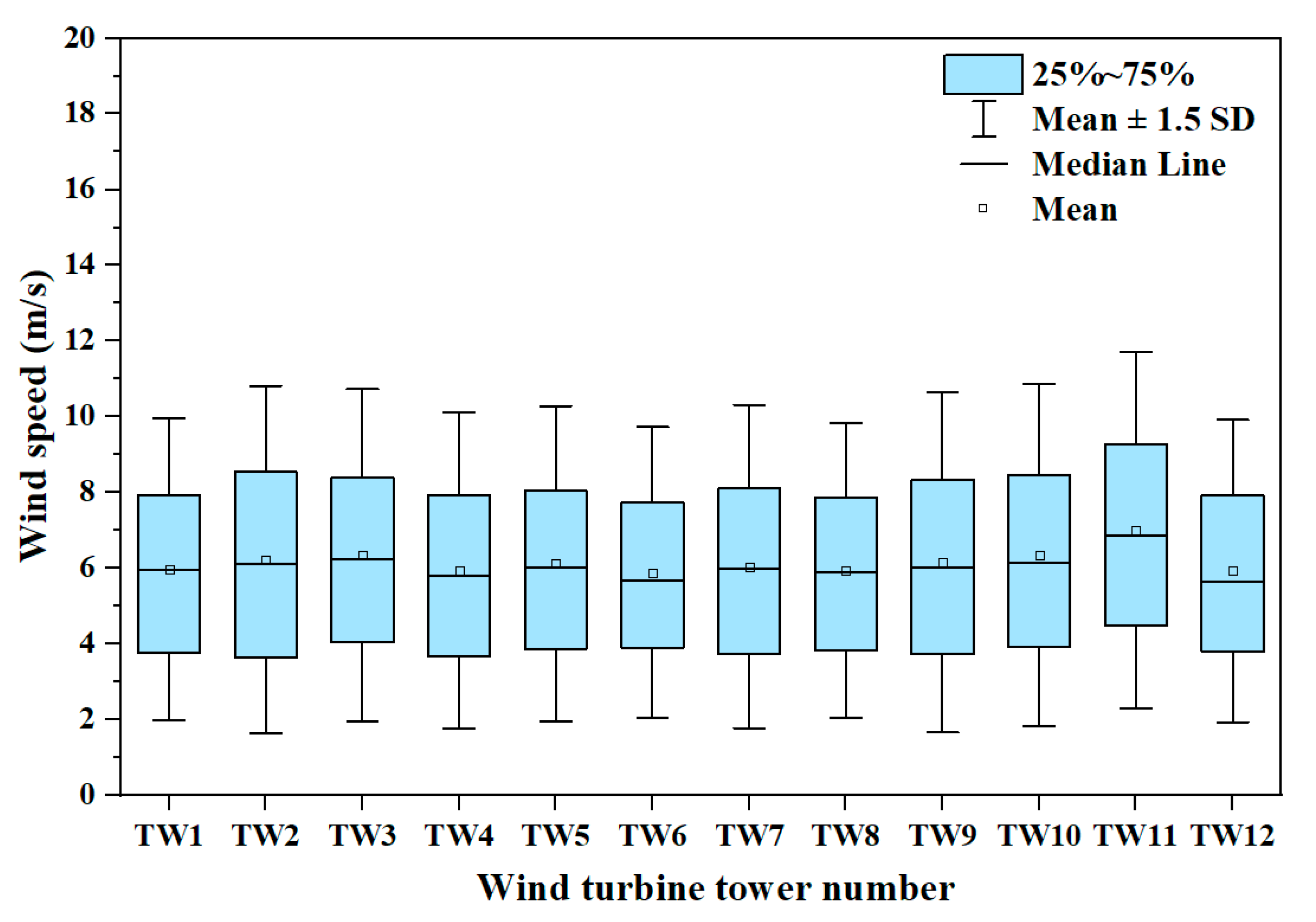
The wind speed data for the entire year of 2022 from the Lamthakhong wind turbine were collected using the WindSCADA system. The objective of this research section is to conduct a statistical analysis to forecast and estimate future wind conditions at the wind turbine farm. Consequently, in the subsequent sections, we will incorporate essential statistical data to fulfill this requirement and advance our understanding of wind dynamics in the region. Therefore, the boxplots of wind speed for all 12 installed wind turbines are depicted in Figure 2, which shows that the average wind speed in the region was approximately 5.5 m/s.

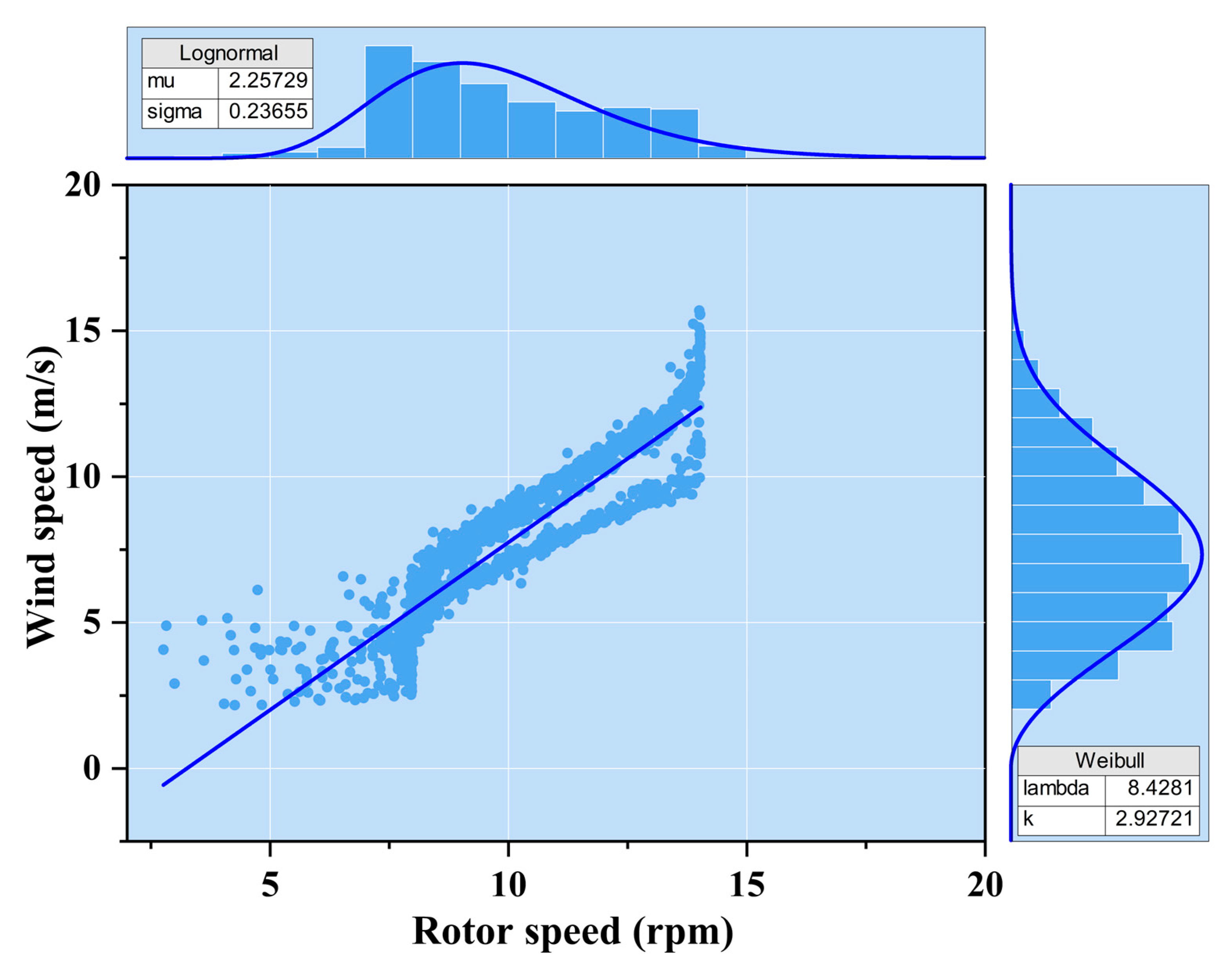
In collaboration with the wind turbine engineering team, three key points of analysis were carefully identified for this study. These points serve as critical thresholds and are crucial for understanding the correlation between wind speed and rotor speed. The minimum threshold was established at 2.5 m/s (4 rpm), at which marginal relaminarization will occur according to Equation (6), creating added complexity in near-wall flow characteristics [32,33], representing the lower limit at which the wind turbine is operational. The midpoint was set at 5.5 m/s (9 rpm), indicating the average wind speed observed during the study period. Finally, the maximum threshold was defined at 10.0 m/s (15 rpm), representing the upper limit beyond which the wind turbine requires protective measures or must be shut down. Figure 3 illustrates these points, providing a visual representation of the linear relationship between wind speed and rotor speed for simulation, validation, and justification purposes.

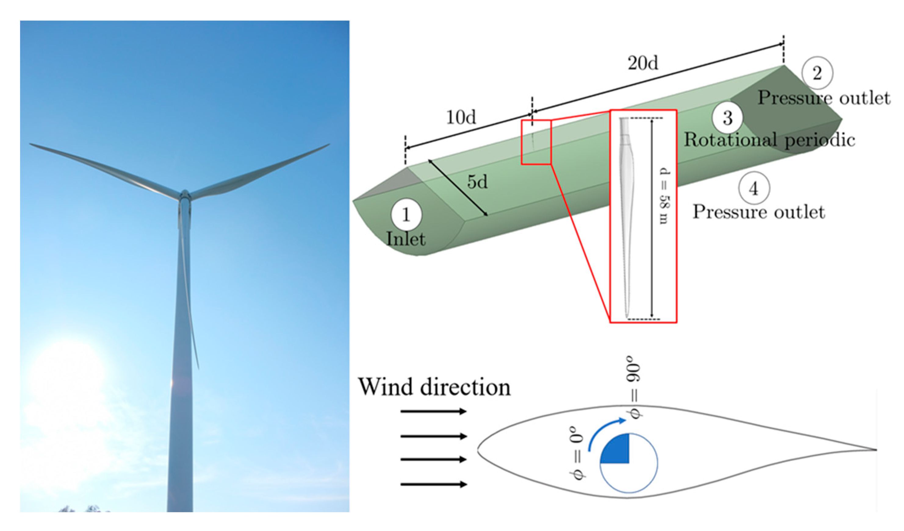
The computational boundary condition used the rotational periodic to reduce the computational time and to satisfy our limited computation resources. Figure 4 describes the domain of the incoming wind speed, the rotational periodic, and the turbine blade direction. In this study, we used ANSYS Fluent 2023R1 to solve the set of fluid dynamics system equations, as shown in Equations (1)–(4). Hybrid Initialization was used in the initial computational solution. With this technique, a collection of recipes and boundary interpolation methods were used. It solved the Laplace equation to produce a velocity field that conforms to wind turbine geometries. All other variables such as turbulence properties were patched based on domain-averaged values [31]. The analysis was run on a system with high-performance parallel computing using a 16 core Intel Xeon [email protected] GHz with 256 Gb of RAM under 24 h operation per the study case.

4.2. Wind Turbine Grid Independence Analysis

Data on the wind speed were collected from the WindSCADA system for the entire year of 2022 (Lamthakhong Wind Turbine Farm, Thailand). The computational grid was divided into two: a global grid indicating the whole computational domain and a local grid point on the investigated surface. This study focused on the blade surface to monitor the grid’s independence. The area-weighted average of a quantity was chosen to validate the solution convergence independence on the number of the grid. Clearly, the area-weighted average is the ratio between summation of the product of the physical variable and the area to sum of the area.

$$\frac{1}{A}{\displaystyle \int {\tau }_w}=\frac{1}{A}{\displaystyle \sum _{i=1}^n{\tau }_{w,i}}\left|A_i\right|$$

(31)

where ${\tau }_{w,i}$ is the wall shear stress of the grid cell on the blade surface and $A_i$ is the local grid cell area. Figure 5 demonstrates that the solution converges when the grid number is between 209,000 and 250,000 cells, with less than a 3% solution change. In this study, we utilized case 5 for all test cases. The grid independence analysis also revealed that although the global cell count was higher in cases 1 and 2, the major variable being investigated still did not converge, with the computation time and resources required being 5–10 times greater than those in cases 4 and 5. Notably, this suggests that the grid independence study must be a compromise between the variable of interest and the global flow field.

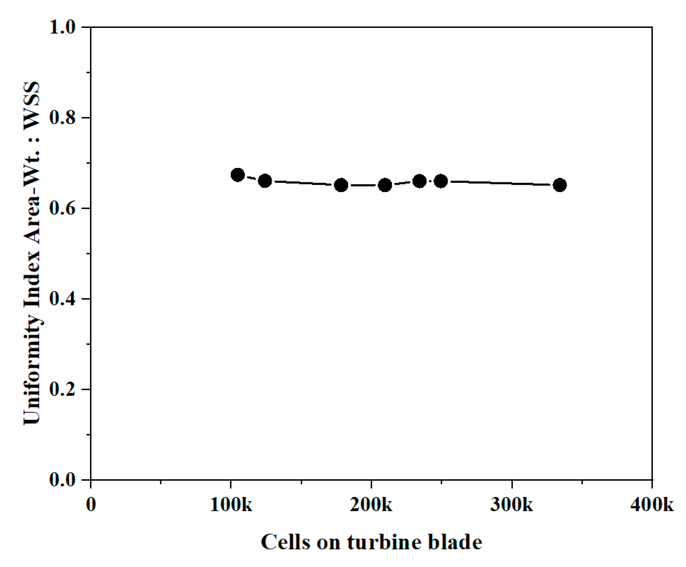
In addition, we monitored local variation distribution for greater consistency of grid independence. The index of uniformity shows the distribution of identified variables over a surface of interest, while the highest uniformity means the index value is close to 1. On the other hand, to observe the variation in selected variables, the area-weighted average is applied to weight the uniformity index. The area-weighted uniformity index $\left({\zeta }_a\right)$ of a variable is computed as

$${\zeta }_a=1-\frac{{\displaystyle \sum _{i=1}^n\left[\left(\left|{\varphi }_i-\overline{{\varphi }_a}\right|A_i\right)\right]}}{2\left|\overline{{\varphi }_a}\right|{\displaystyle \sum _{i=1}^n{A}_i}}$$

(32)

where $i$ is the facet index of a surface with $n$ facets and $\overline{{\varphi }_a}$ is the average value of the field variable over the surface:

$$\overline{{\varphi }_a}=\frac{{\displaystyle \sum _{i=1}^n{\varphi }_i{A}_i}}{{\displaystyle \sum _{i=1}^n{A}_i}}$$

(33)

The results presented in Figure 6 demonstrate the precision of the uniformity index during the grid independence analysis. It is evident that case 5 had the most favorable variation in uniformity. Considering both the global and local investigations conducted, case 5 was selected as the representative case for all subsequent studies in the grid independence analysis. This decision was based on the superior performance and consistency demonstrated by case 5 in terms of achieving grid-independent results. By utilizing case 5 as a reference, further studies and simulations can be conducted with confidence, ensuring reliable and accurate outcomes. The grid is shown in Figure 7.

4.3. Validation Study

The study results were compared with measured site data from the EGAT WindSCADA system for computational validation. The performance levels of power outputs are described in terms of torque, computed using procedures described in the ANSYS Fluent manual and theory guide [31]. The total torque vector about the rotor axis is calculated by summing the elemental cross products of the pressure and viscous force vectors times the vector $\overrightarrow{r}$. Equation (34) represents the pressure and viscous torque vector:

$$\overrightarrow{{\rm T}}\left(\theta \right)=\overrightarrow{r}\times {\overrightarrow{F}}_p\left(\theta \right)+\overrightarrow{r}\times {\overrightarrow{F}}_v\left(\theta \right)$$

(34)

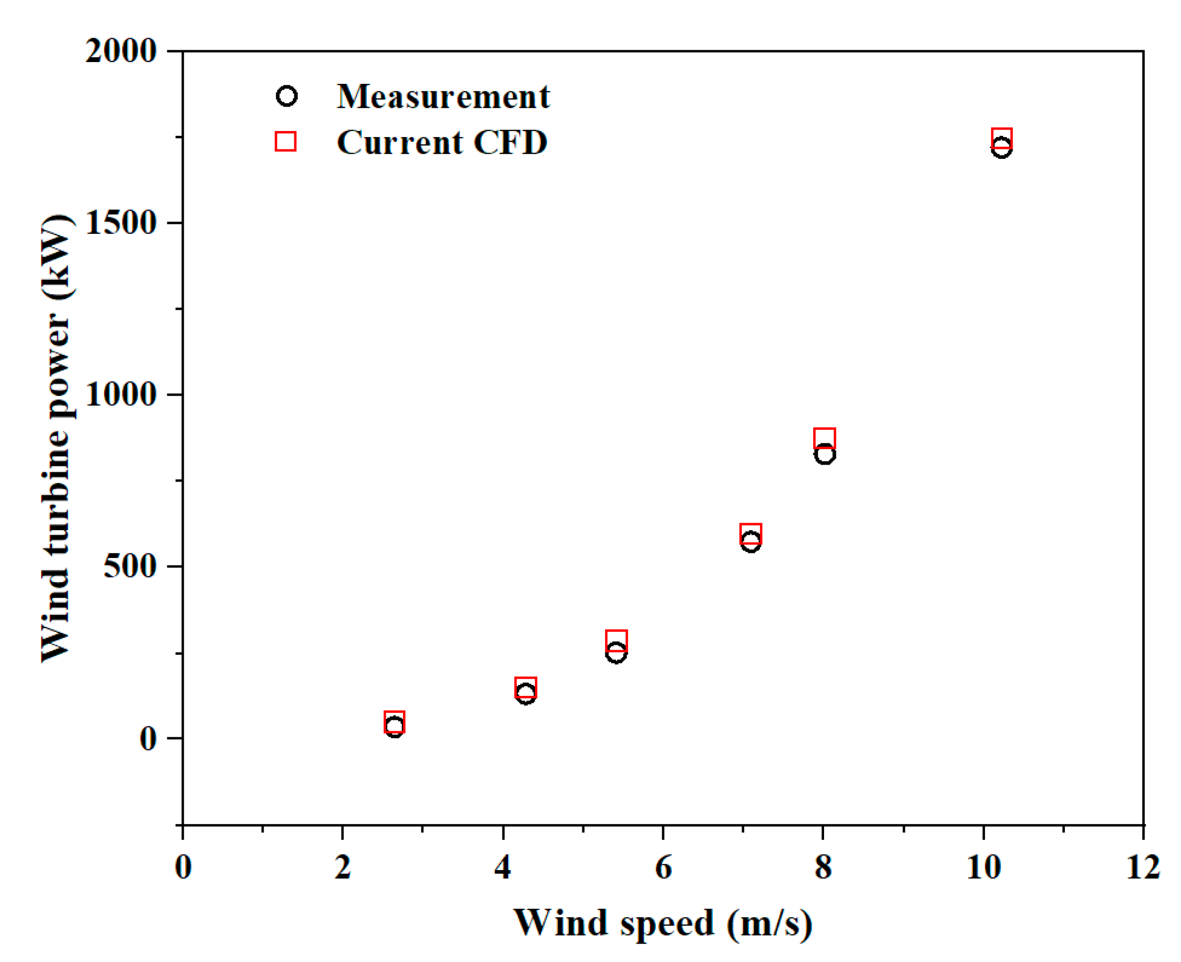
where ${\overrightarrow{F}}_p$ is the pressure force vector, ${\overrightarrow{F}}_v$ is the viscous force vector, and $\overrightarrow{r}$ is the blade diameter. The validation of measurements compared to the current CFD output is shown in Figure 8, confirming that the geometry, grid analysis, boundary condition, mathematical setting, and initial conditions were consistent with actual flow physics.

5. Results

This investigation aimed to predict realistic wind turbine blades through computational fluid dynamics based on wall shear stress. The geometry was produced from high-precision 3D laser scanning. The boundary condition was measured using the WindSCADA system, installed on an EGAT wind turbine farm and validated based on numerical analysis and field measurements. The investigation results in Figure 8 confirmed that all our settings represented realistic flow physics and were suitable for highly accurate interpretation, as discussed in the following section.

5.1. Incoming Wind Speed Distribution and Statistical Analysis

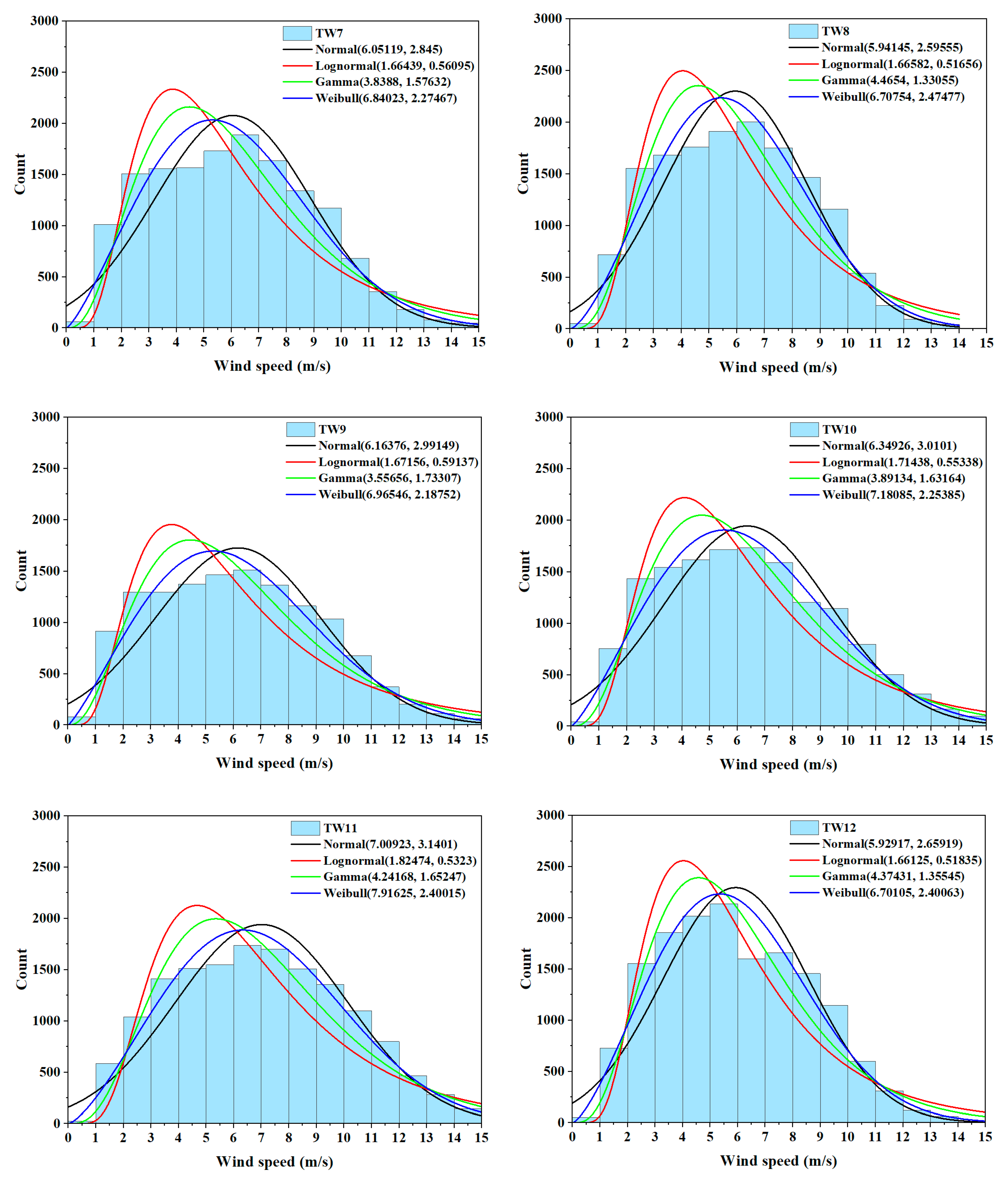
In this study, our objective was to assess the wind distribution at a specific location. While research papers commonly apply the Weibull distribution to represent incoming wind speed [11,34], it is essential to consider that wind distribution can vary depending on specific factors, such as geography, proximity to the equator, sea level, and local terrain. To address this, we utilized the MINITAB R21 software to test the incoming wind speed distribution. The Anderson–Darling test was selected as the main parameter to interpret and validate the distribution shape [35]. Through statistical analysis, the distribution was plotted, and the goodness of fit was assessed, as presented in

Table 2. Anderson–Darling test data for goodness of fit test.

Distribution	TW1	TW2	TW3	TW4	TW5	TW6	TW7	TW8	TW9	TW10	TW11	TW12
Normal	46.33	55.65	27.29	55.47	53.47	50.85	59.50	53.58	57.52	68.42	47.73	76.36
Lognormal	221.86	162.30	128.91	168.41	185.66	154.75	228.87	214.28	193.67	163.35	207.80	151.74
Weibull	36.58	38.36	11.07	20.52	20.86	12.95	36.55	33.52	30.24	18.20	20.59	26.20
Gamma	106.78	79.59	50.70	67.46	76.21	56.12	103.70	101.50	83.47	59.96	85.24	61.62

, providing crucial metrics for evaluating the accuracy and suitability of the distribution model in capturing the wind behavior at the study location.

Based on the Anderson–Darling test for goodness of fit, the statistical analysis reveals that the incoming airflow distribution across the different states listed in Table 2 is best represented by the Weibull distribution. This finding aligns with other research studies, confirming the global trend that the incoming wind distribution at the Lamthakhong Wind Farm can be represented using a Weibull function [36,37]. The distribution histogram, depicted in Figure 9, illustrates the results of the statistical analysis for all wind turbine towers. Understanding and focusing on this distribution pattern is of the utmost importance for accurate wind forecasting and estimation. This finding will guide future investigations and prediction scenario analyses specifically tailored to the Lamthakhong Wind Farm, enabling more precise assessments and predictions of wind behavior in the area.

5.2. Effect of Transition Turbulence Model

This study investigated wind turbines operating in a 2.5–10 m/s wind speed range. However, due to the transitional flow regime at low Reynolds numbers, the SST k-ω turbulence model’s ability to accurately predict performance within this range is uncertain according to the inclusion in SST k-ω of a destruction and relaminarization term, as shown in Equations (6)–(30). This additional turbulence mathematical model aims to improve the characteristic flow mix between turbulence and laminar, which expects good computational results in a low-speed flow or a high pitch angle (PA). However, to test this hypothesis for this study, we compared the SST k-ω model with the transition SST model.

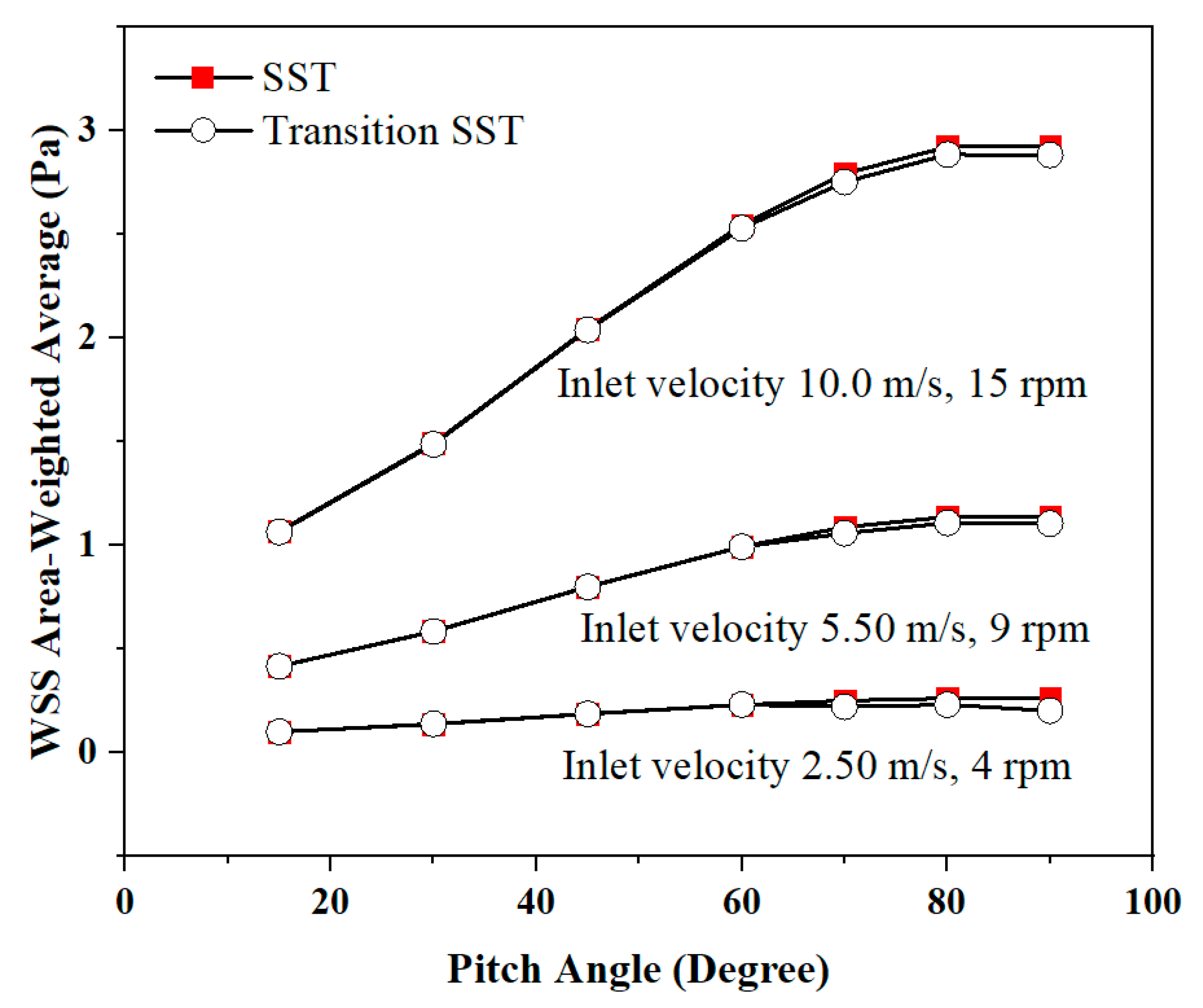
In conclusion, the comparison of the wall shear stress weighted average between the SST k-ω and transition SST turbulence models, as presented in Figure 10, indicates several substantial differences overall for this study (less than 5% for all cases). However, a slight distinction was observed at different PA values for all incoming air velocity. This finding holds particular importance for wind farms operating under high PA conditions and for the inspection area by maintenance technicians. Physically, the k-ω turbulence model in CFD methods is the classical turbulence model for studying airfoils. The advantages and improvements in the computational method proposed in this paper compared with the previous method still need more validation and verification.

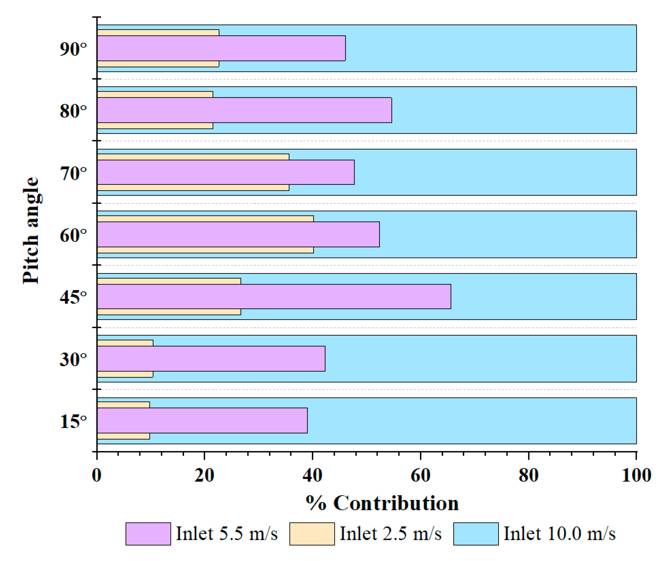
Incorporating this insight into performance analysis systems is crucial, as it enables the development of monitoring systems tailored to existing wind farms. By leveraging this knowledge, these monitoring systems can effectively evaluate and manage the impact of a high PA on wind turbine performance, optimizing overall operational efficiency, safety, and yearly preventive maintenance. In addition, the incoming air velocity is the main parameter that affects the wall shear stress on the turbine blade, as shown in Figure 11. If we set the maximum contribution of the incoming wind velocity as the baseline and express the others as a percentage of this value, we find that at a wind speed of 2.5 m/s and 4 rpm, the contribution is 12–40%, and the maximum wall shear stress occurs at a PA of 60°. This approximates the case of an incoming air velocity of 5.5 m/s and 9 rpm, where the maximum wall shear stress occurs at a PA of 45°, with a contribution of 70%. However, the relationship between incoming air velocity and wall shear stress does not follow a linear trend. This finding is important for wind turbine farms, as it can be used to estimate wind power and prioritize maintenance schedules to monitor the possibility of blade delamination. This is a topic that is currently being researched by an EGAT team.

5.3. Wall Shear Stress Distribution Compared with Current Damage

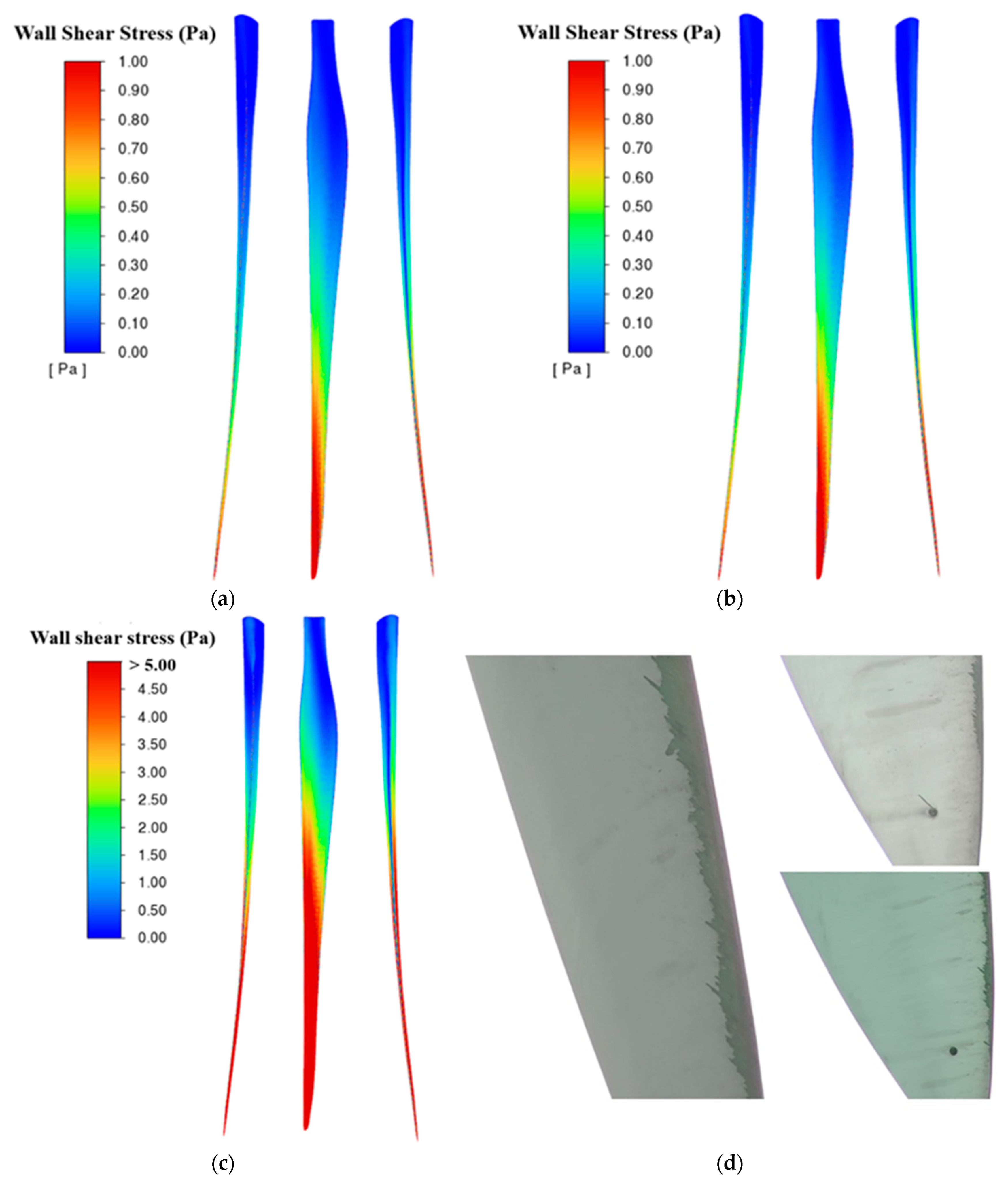
The difficulty of calculating wind turbine damage is more challenging since it involves chaotic flow physics, anisotropic composite materials, and structural design. As a result, this study will present an indirect hypothesis for estimating it using wall shear stress, as demonstrated in Equation (5). The essential contribution is wind velocity, which we can obtain via the WindSCADA system. To establish the correctness of this hypothesis, we must observe the damage at the same region of high wall shear stress. However, the damage mechanism was not included in this study. The CFD analysis depicted in Figure 12 reveals that the wall shear stress distribution indicates elevated values at the leading edge of the wind turbine blade (five times increasing when air velocity 2.50 m/s, 4 rpm increase to 10.00 m/s, 15 rpm), suggesting a higher likelihood of damage in that region compared to other areas. In this analysis, we focused on a specific case illustrated in Figure 10, where the turbine blade experienced increased wall shear stress. By comparing the computational results with the existing damage, we were able to observe a consistent pattern, with the tip of the blade showing both high wall shear stress and damage. Consequently, we can conclude that wall shear stress serves as a reliable predictor of blade surface delamination and associated damage. These results, like the mechanism described in other research [38,39,40], give us confidence that all our settings are correct and that we have obtained numerical fidelity in the results. Therefore, our simulated results are very important for the Lamthakhong Wind Farm as they enable the implementation of an effective preventive maintenance strategy. By utilizing the insights from this research, the Wind Farm can establish a schedule for planning and make further predictions based on CFDs simulations to mitigate potential damage.

5.4. Preventive Maintenance Schedule Planning for Delamination and Corrosion

Preventive maintenance schedule planning for delamination and corrosion based on wall shear stress predicted using CFDs involves leveraging the predictive capabilities of CFDs simulations to identify critical areas prone to damage. By analyzing the wall shear stress distribution obtained from CFDs models, regions with elevated wall shear stress can be identified, indicating potential areas susceptible to delamination and corrosion. The annual variation in wind patterns can be described, based on the wind data collected throughout the entire year, as depicted in Figure 13. The analysis revealed that the period from June to October experiences higher wind speeds and greater fluctuations than in other months. Therefore, it is advisable to monitor flow-induced delamination damage before June as a reference point rather than comparing it with observations made after October when the wind conditions are less severe. This approach facilitates identifying and assessing delamination occurrences by establishing a baseline during heightened wind activity.

Incorporating this information into the maintenance schedule planning would allow for targeted inspections, maintenance, and protective measures in those high-risk areas. Proactively addressing these areas with appropriate treatments, coatings, or repairs can mitigate the detrimental effects of delamination and corrosion, optimizing the lifespan and performance of the equipment or structure. This approach enables efficient allocation of resources and minimizes downtime, ensuring the long-term reliability and safety of the system.

The final discussion with the wind turbine engineering staff at the Wind Farm resulted in the design and description of an appropriate drone inspection procedure, as outlined in Figure 14. Our findings reveal that the current drone inspection protocol did not incorporate the wind data presented in Figure 13 or consider the location of wall shear stress. Consequently, the inspection protocol begins at the blade tip, considering the highest wall shear stress, progresses to the leading edge, upper, and lower surfaces, and finally inspects the trailing edge. The implemented drone inspection procedure has been proven effective and reliable. This procedure further confirmed the importance of the wall shear stress distribution in predicting delamination and corrosion. In addition, the wall shear stress observed in the blade region serves as a valuable input for developing preventive maintenance procedures that align well with the drone inspection process. As a result, this research has yielded successful outcomes with practical implications for real-world applications, as well as sustainability in developing a specific yearly maintenance protocol and strategies for human development in future investigation projects at Lamthakhong Wind Turbine Farm.

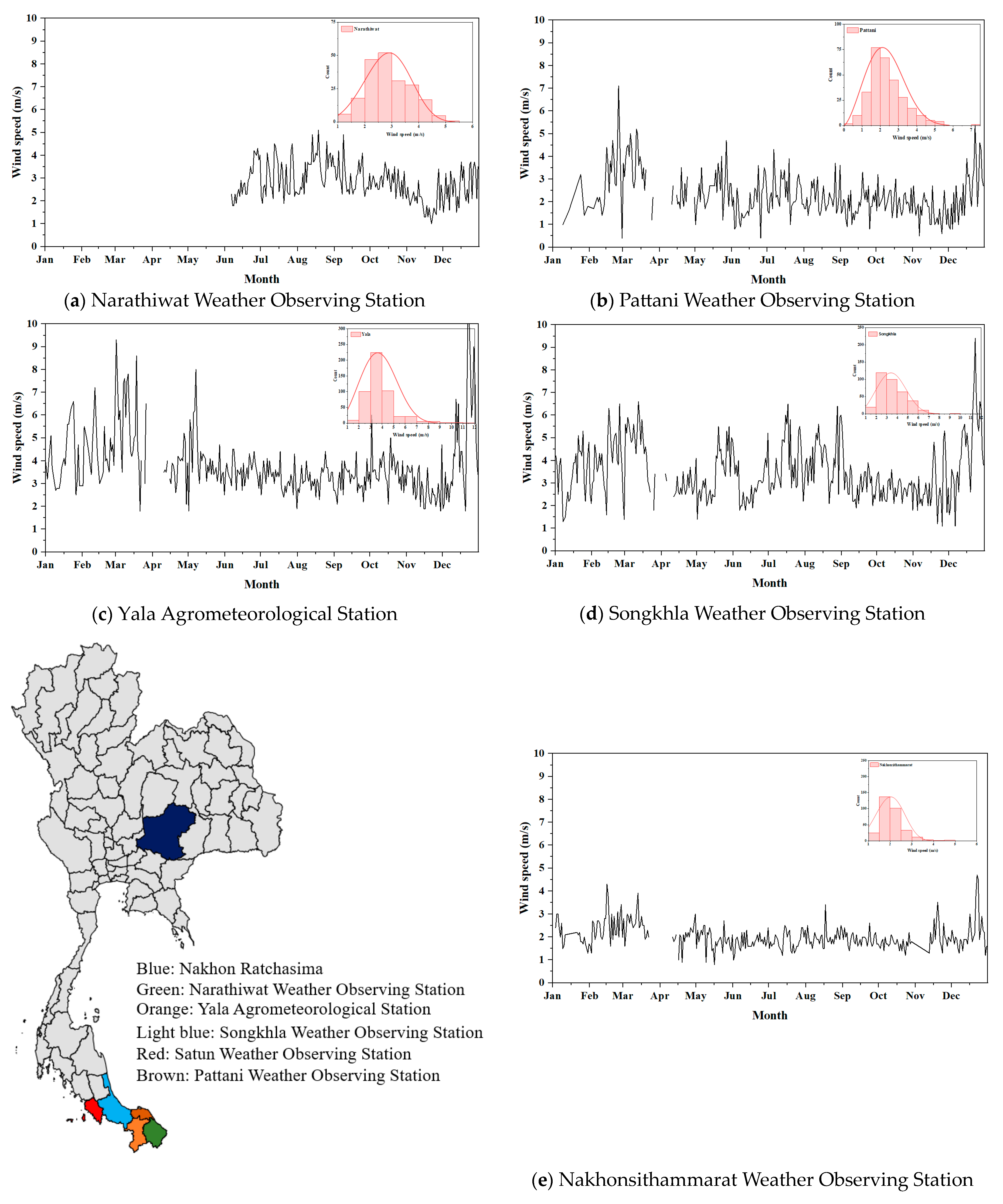
In 2024, with a focus on enhancing human and social sustainability, we have broadened our exploration of wind behavior at Thailand’s Lamthakhong Wind Turbine Farm in Nakhon Ratchasima Province. Following the successful implementation of a new technique and receiving favorable feedback from inspection specialists, we have utilized surface wind speed data from the Thai methodological department to expand our discoveries, as depicted in Figure 15. Initially, our observation efforts commenced in Southern Thailand to track the fluctuation in wind speed over time. However, certain data points were lost during the monsoon day. Our analysis indicated significant variation in the peak surface wind speeds based on location, with the distribution of wind speeds remaining consistent with a Weibull distribution. Additionally, the coastal regions in Southern Thailand present favorable conditions for the installation of wind turbine farms. While large-scale power systems are necessary, medium-sized systems suffice for sustaining agricultural activities in smaller settlements. The distinctive characteristics of coastal areas, coupled with significant fluctuations in wind speed during the monsoon season, influence wind dynamics that potentially lead to damage to wind turbine systems or coastal beaches [41]. This discovery underscores the importance of prior knowledge in managing wind farms and lays a foundation for future wind turbine implementations, as well as being valuable for guiding specific preventive maintenance and inspection protocols. Moreover, engineers and inspection specialists must possess a comprehensive understanding of local wind dynamics before employing any particular procedure. Lastly, studies conducted at the Lamthakhong Wind Turbine Farm highlight the significance of incoming airflow, which is closely linked to issues like blade delamination and corrosion induced by high wall shear stress, especially at the blade tip and leading edge. Given the substantial fluctuations in surface wind speed observed in Southern Thailand, there is a pressing need for stricter monitoring and the adoption of efficient maintenance techniques.

6. Conclusions

This study applied a numerical simulation technique to predict the wall shear stress that induces delamination and erosion on wind turbine blades. The grid independence tests both global and local regions to ensure all grid points are presented. The turbulence model SST k-ω is used, while the transition SST is also used to compare performance. To enhance further prediction, statistical analysis should be applied to acquire more detail in the interpretation of the results. The conclusions from the study are

(1)

Based on the Anderson–Darling test for goodness of fit, the statistical analysis indicated that the incoming airflow distribution at the Lamthakhong wind farm, as depicted in Table 2 and Figure 9, is best represented by the Weibull distribution. This finding aligns with other research, suggesting that the global trend of the Weibull function applies to the wind distribution for this wind farm. Understanding the characteristics of this distribution is needed for precise wind forecasting, estimation, and conducting future investigations and scenario analyses specific to the Lamthakhong Wind Farm. By considering the Weibull distribution, more accurate predictions and assessments can be made, aiding in optimizing operations and decision-making processes related to the Wind Farm.

(2)

The comparison between the SST k-ω and transition SST turbulence models in Figure 10 suggests no significant differences for the low pitch angle (PA) case, but a slight difference was observed at a high pitch angle. This finding is important for wind farms operating under high-pitch angle conditions and in designing airfoil shapes that need to account for this effect.

(3)

By comparing the computational results with the existing damage in Figure 12d, we were able to observe a consistent pattern, with the tip of the blade exhibiting both high wall shear stress and damage. Consequently, we can conclude that wall shear stress serves as a reliable predictor of blade surface delamination and associated damage.

(4)

Our prediction, that wall shear stress varies with inlet velocity as shown in Equation (5) and Figure 11, suggests that incoming air speed can be used to determine wall shear stress levels. Therefore, precise data from the WindSCADA system can be used for the future assessment of wall shear stress levels.

(5)

Based on the wind data collected throughout the entire year, as depicted in Figure 13, it is advisable to conduct monitoring for flow-induced delamination damage prior to June as a reference point, rather than comparing it with observations made after October when the wind conditions are less severe. Unique protocols are established for internal yearly maintenance improvement.

(6)

The analysis of surface wind speed in Southern Thailand in Figure 15 reveals heightened fluctuations influenced by both the monsoon season and coastal geography. As a result, an effective maintenance protocol capable of accommodating these conditions is required.

(7)

It is crucial to prioritize future enhancements in inspection methods to ensure ongoing efficiency and effectiveness. These improvements are essential for both the ongoing research projects in the Lamthakhong Wind Farm and Southern Thailand.

References

1. Akhter, M.Z.; Ali, A.R.; Jawahar, H.K.; Omar, F.K.; Elnajjar, E. Enhanced energy extraction in small-scale wind turbines through slot-based passive blowing. Energy Convers. Manag. X 2023, 19, 100400. [Google Scholar] [CrossRef]
2. Huang, S.; Qiu, H.; Wang, Y. Aerodynamic performance of horizontal axis wind turbine with application of dolphin head-shape and lever movement of skeleton bionic airfoils. Energy Convers. Manag. 2022, 267, 115803. [Google Scholar] [CrossRef]
3. Cai, X.; Gu, R.; Pan, P.; Zhu, J. Unsteady aerodynamics simulation of a full-scale horizontal axis wind turbine using CFD methodology. Energy Convers. Manag. 2016, 112, 146–156. [Google Scholar] [CrossRef]
4. Giahi, M.H.; Jafarian Dehkordi, A. Investigating the influence of dimensional scaling on aerodynamic characteristics of wind turbine using CFD simulation. Renew. Energy 2016, 97, 162–168. [Google Scholar] [CrossRef]
5. Elsakka, M.M.; Ingham, D.B.; Ma, L.; Pourkashanian, M. CFD analysis of the angle of attack for a vertical axis wind turbine blade. Energy Convers. Manag. 2019, 182, 154–165. [Google Scholar] [CrossRef]
6. Nejadkhaki, H.K.; Sohrabi, A.; Purandare, T.P.; Battaglia, F.; Hall, J.F. A variable twist blade for horizontal axis wind turbines: Modeling and analysis. Energy Convers. Manag. 2021, 248, 114771. [Google Scholar] [CrossRef]
7. Regodeseves, P.G.; Morros, C.S. Numerical study on the aerodynamics of an experimental wind turbine: Influence of nacelle and tower on the blades and near-wake. Energy Convers. Manag. 2021, 237, 114110. [Google Scholar] [CrossRef]
8. Zhang, R.; Xin, Z.; Huang, G.; Yan, B.; Zhou, X.; Deng, X. Characteristics and modelling of wake for aligned multiple turbines based on numerical simulation. J. Wind Eng. Ind. Aerodyn. 2022, 228, 105097. [Google Scholar] [CrossRef]
9. Steiner, J.; Dwight, R.P.; Viré, A. Data-driven RANS closures for wind turbine wakes under neutral conditions. Comput. Fluids 2022, 233, 105213. [Google Scholar] [CrossRef]
10. Boye, T.E.; Xie, Z.T. Aerodynamics of a pitching wind turbine blade at high reduced frequencies. J. Wind Eng. Ind. Aerodyn. 2022, 223, 104935. [Google Scholar] [CrossRef]
11. Kelly, J.; Vogel, C.; Willden, R. Impact and mitigation of blade surface roughness effects on wind turbine performance. Wind Energy 2022, 25, 660–677. [Google Scholar] [CrossRef]
12. Solomin, E.V.; Terekhin, A.A.; Martyanov, A.S.; Shishkov, A.N.; Kovalyov, A.A.; Ismagilov, D.R.; Ryavkin, G.N. Horizontal axis wind turbine yaw differential error reduction approach. Energy Convers. Manag. 2022, 254, 115255. [Google Scholar] [CrossRef]
13. Li, C.; Abraham, A.; Li, B.; Hong, J. Incoming flow measurements of a utility-scale wind turbine using super-large-scale particle image velocimetry. J. Wind Eng. Ind. Aerodyn. 2020, 197, 104074. [Google Scholar] [CrossRef]
14. Gao, L.; Yang, S.; Abraham, A.; Hong, J. Effects of inflow turbulence on structural response of wind turbine blades. J. Wind Eng. Ind. Aerodyn. 2020, 199, 104137. [Google Scholar] [CrossRef]
15. Guo, T.; Guo, X.; Gao, Z.; Li, S.; Zheng, X.; Gao, X.; Li, R.; Wang, T.; Li, Y.; Li, D. Nacelle and tower effect on a stand-along wind turbine energy output—A discussion on field measurements of a small wind turbine. Appl. Energy 2021, 303, 117590. [Google Scholar] [CrossRef]
16. Zhang, Y.; Zhang, Z.; Zheng, J.; Zhang, J.; Zheng, Y.; Zang, W.; Lin, X.; Fernandez-Rodriguez, E. Experimental investigation into effects of boundary proximity and blockage on horizontal-axis tidal turbine wake. Ocean Eng. 2021, 225, 108829. [Google Scholar] [CrossRef]
17. Neunaber, I.; Hölling, M.; Whale, J.; Peinke, J. Comparison of the turbulence in the wakes of an actuator disc and a model wind turbine by higher order statistics: A wind tunnel study. Renew. Energy 2021, 179, 1650–1662. [Google Scholar] [CrossRef]
18. Li, Q.; Wang, Y.; Kamada, Y.; Maeda, T.; Xu, J.; Zhou, S.; Zhang, F.; Cai, C. Diagonal inflow effect on the wake characteristics of a horizontal axis wind turbine with Gaussian model and field measurements. Energy 2022, 238, 121692. [Google Scholar] [CrossRef]
19. Das, T.K.; Kundu, D. Feasibility and sensitivity analysis of a self-sustainable hybrid system: A case study of a mountainous region in Bangladesh. Energy Convers. Manag. X 2023, 20, 100411. [Google Scholar] [CrossRef]
20. Taoufik, M.; Fekri, A. GIS-based multi-criteria analysis of offshore wind farm development in Morocco. Energy Convers. Manag. X 2021, 11, 100103. [Google Scholar] [CrossRef]
21. Eikeland, O.F.; Hovem, F.D.; Olsen, T.E.; Chiesa, M.; Bianchi, F.M. Probabilistic forecasts of wind power generation in regions with complex topography using deep learning methods: An Arctic case. Energy Convers. Manag. X 2022, 15, 100239. [Google Scholar] [CrossRef]
22. Dashtkar, A.; Hadavinia, H.; Sahinkaya, M.N.; Williams, N.A.; Vahid, S.; Ismail, F.; Turner, M. Rain erosion-resistant coatings for wind turbine blades: A review. Polym. Polym. Compos. 2019, 27, 443–475. [Google Scholar] [CrossRef]
23. Johansen, N.F.J.; Mishnaevsky, L.; Dashtkar, A.; Williams, N.A.; Fæster, S.; Silvello, A.; Cano, I.G.; Hadavinia, H. Nanoengineered graphene-reinforced coating for leading edge protection of wind turbine blades. Coatings 2021, 11, 1104. [Google Scholar] [CrossRef]
24. Nash, D.; Leishman, G.; Mackie, C.; Dyer, K.; Yang, L. A Staged Approach to Erosion Analysis of Wind Turbine Blade Coatings. Coatings 2021, 11, 681. [Google Scholar] [CrossRef]
25. Herring, R.; Domenech, L.; Renau, J.; Šakalytė, A.; Ward, C.; Dyer, K.; Sánchez, F. Assessment of a Wind Turbine Blade Erosion Lifetime Prediction Model with Industrial Protection Materials and Testing Methods. Coatings 2021, 11, 767. [Google Scholar] [CrossRef]
26. Obanijesu, E.O. Modeling the H2S contribution to internal corrosion rate of natural gas pipeline. Energy Sources Part A Recovery Util. Environ. Eff. 2009, 31, 348–363. [Google Scholar] [CrossRef]
27. Madasamy, P.; Chandramohan, P.; Mukunthan, M.; Krishna Mohan, T.V.; Rangarajan, S.; Uttam, N.; Ramakrishnan, R.; Babulal, G.; Rani, H.P.; Surendran, P.; et al. Flow accelerated corrosion rate on carbon steel pipe bend by thin layer activation technique and computational modeling: Under PHWR operating conditions. Eng. Fail. Anal. 2021, 121, 105125. [Google Scholar] [CrossRef]
28. Dimitrova, M.; Aminzadeh, A.; Meiabadi, M.S.; Sattarpanah Karganroudi, S.; Taheri, H.; Ibrahim, H. A Survey on Non-Destructive Smart Inspection of Wind Turbine Blades Based on Industry 4.0 Strategy. Appl. Mech. 2022, 3, 1299–1326. [Google Scholar] [CrossRef]
29. Castorrini, A.; Ortolani, A.; Campobasso, M.S. Assessing the progression of wind turbine energy yield losses due to blade erosion by resolving damage geometries from lab tests and field observations. Renew. Energy 2023, 218, 119256. [Google Scholar] [CrossRef]
30. Menter, F.R.; Langtry, R.B.; Likki, S.R.; Suzen, Y.B.; Huang, P.G.; Völker, S. A correlation-based transition model using local variables—Part I: Model formulation. J. Turbomach. 2006, 128, 413–422. [Google Scholar] [CrossRef]
31. Ansys Fluent. ANSYS Fluent Theory Guide (2023R1); ANSYS Inc.: Canonsburg, PA, USA, 2023. [Google Scholar]
32. Kaewbumrung, M.; Plengsa-Ard, C. Numerical simulation of jet impingement relaminarization using nonlinear eddy viscosity turbulence models. Eng. Appl. Comput. Fluid Mech. 2023, 17, e2162132. [Google Scholar] [CrossRef]
33. Kaewbumrung, M.; Plengsa-Ard, C. Relaminarization of jet impingement on a flat plate using separation-induced transition correction turbulence modeling preliminarily applied in archeological applications. Heliyon 2024, 10, e26040. [Google Scholar] [CrossRef] [PubMed]
34. Gualtieri, G.; Secci, S. Extrapolating wind speed time series vs. Weibull distribution to assess wind resource to the turbine hub height: A case study on coastal location in Southern Italy. Renew. Energy 2014, 62, 164–176. [Google Scholar] [CrossRef]
35. Jung, C.; Schindler, D.; Buchholz, A.; Laible, J. Global gust climate evaluation and its influence on wind turbines. Energies 2017, 10, 1474. [Google Scholar] [CrossRef]
36. Pobočíková, I.; Michalková, M.; Sedliačková, Z.; Jurášová, D. Modelling the Wind Speed Using Exponentiated Weibull Distribution: Case Study of Poprad-Tatry, Slovakia. Appl. Sci. 2023, 13, 4031. [Google Scholar] [CrossRef]
37. Derome, D.; Razali, H.; Fazlizan, A.; Jedi, A. Distribution cycle of wind speed: A case study in the Southern Part of Malaysia. IOP Conf. Ser. Mater. Sci. Eng. 2023, 1278, 012010. [Google Scholar] [CrossRef]
38. Wang, Y.; Wu, C.; Zhao, S.; Guo, Z.; Zu, B.; Han, M.; Du, Q.; Ni, M.; Jiao, K. Assessing performance degradation induced by thermal cycling in solid oxide cells. Energy Convers. Manag. 2022, 270, 116239. [Google Scholar] [CrossRef]
39. Gu, Y.; Nguyen, T.; Donough, M.J.; Gangadhara Prusty, B.; Wang, J. Mechanisms of pop-up delamination in laminated composites pierced by the initial pure waterjet in abrasive waterjet machining. Compos. Struct. 2022, 297, 115968. [Google Scholar] [CrossRef]
40. Liu, J.W.; Liu, P.F.; Leng, J.X.; Wang, C.Z. Finite element analysis of damage mechanisms of composite wind turbine blade by considering fluid/solid interaction. Part I: Full-scale structure. Compos. Struct. 2022, 301, 116212. [Google Scholar] [CrossRef]
41. Thongsri, J.; Tangsopa, W.; Kaewbumrung, M.; Phanak, M.; Busayaporn, W. Derosion Lattice Performance and Optimization in Solving an End Effect Assessed by CFD: A Case Study in Thailand’s Beach. Water 2022, 14, 1358. [Google Scholar] [CrossRef]
Figure 1. Three-dimensional high-precision geometry of finished surface. (a) FARO Laser Scanner Focus3D with 15 locations for scanning; (b) full model of raw point cloud data; (c) 3D-CAD model.
Sustainability 16 02873 g001
Figure 2. Wind speed at Lamthakhong Wind Farm.
Sustainability 16 02873 g002
Figure 3. Relationship between wind speed and rotor speed.
Sustainability 16 02873 g003
Figure 4. Computational simulation domain.
Sustainability 16 02873 g004
Figure 5. Grid independence analysis.
Sustainability 16 02873 g005
Figure 6. Grid independence analysis using wall shear stress uniformity index.
Sustainability 16 02873 g006
Figure 7. Computational grid using Hybrid MOSAIC meshing technology.
Sustainability 16 02873 g007
Figure 8. Wind turbine power output validation.
Sustainability 16 02873 g008
Figure 9. Incoming wind speed distribution for different wind towers.
Sustainability 16 02873 g009aSustainability 16 02873 g009b
Figure 10. Wall shear stress comparison between SST k-ω and transition SST models.
Sustainability 16 02873 g010
Figure 11. Wall shear stress contribution for different incoming air velocities.
Sustainability 16 02873 g011
Figure 12. Wind turbine damage compared with wall shear stress. (a) PA 90°, incoming air velocity 2.50 m/s, 4 rpm; (b) PA 90°, incoming air velocity 5.50 m/s, 9 rpm; (c) PA 90°, incoming air velocity 10.00 m/s, 15 rpm; (d) current damage on wind turbine blade (2023).
Sustainability 16 02873 g012
Figure 13. Wind data collected throughout entire year (2022).
Sustainability 16 02873 g013
Figure 14. Preventive maintenance inspection areas for drone.
Sustainability 16 02873 g014
Figure 15. Local surface wind speed in Southern Thailand (Jan 2023–Jan 2024).
Sustainability 16 02873 g015