Abstract
In order to optimize the structure of a subway shield tunnel, minimize injuries, and avoid potential safety hazards, the lateral convergence deformation of subway shield tunnels should be predicted. In terms of accuracy and stability, existing prediction models perform poorly in obtaining the lateral convergence deformation value of a non-stationary small-sized sample of a subway shield tunnel. In this paper, a lateral convergence model of a subway shield tunnel based on the Kalman algorithm is constructed based on Kalman filtering theory. The model is efficient, adaptive, and robust and can accurately predict the lateral convergence deformation of a subway shield tunnel. Taking the horizontal diameter of a 200-ring shield segment in the interval section of a subway tunnel as an example, we have proved that the residuals of the Kalman prediction model are small, the residual distribution conforms to the normal distribution, and the prediction effect is great. The model is suitable for the prediction of more than five periods of data, and the prediction accuracy of the model improves with an increase in the number of data periods. In addition, in this paper, we compare the Kalman model with the GM(1,1) model and the GM–Markov model, and the RMSE, NRMSE, MAPE, and R2 are used as evaluation indices. The results show that the Kalman model has a higher prediction accuracy and is more suitable for predicting the lateral convergence deformation of a subway shield tunnel.
1. Introduction
In recent years, with China’s strong support for the development and utilization of underground space, an increasing number of subway lines have started operating, and the safety and health problems of subway tunnels have gradually come into focus. Shield tunneling is the most commonly used method for the construction of subway tunnels. Great attention should be paid to the structural safety of subway tunnels using this method; such tunnels have a long life cycle, complex project operation, large investment, and high risk. The lateral convergence deformation of a tunnel during operation is a key index of the current status of a tunnel structure, and it is also an important part of tunnel monitoring. On one hand, the lateral convergence deformation of a subway shield tunnel will gradually increase with an increase in its service life. Excessive lateral deformation will cause concrete crushing, joint leakage, bolt yielding, and insufficient limits, which can damage the structure of the tunnel and affect its operational safety [1]. On the other hand, with the increase in the quantity of subway lines, it is inevitable that loading and unloading construction activities must be carried out around built interval tunnels, such as the construction of high-rise buildings or the excavation of adjacent tunnels. These behaviors may cause a large lateral deformation of the tunnel, posing a threat to the safety of the tunnel’s structure. Predicting the lateral convergence deformation of subway shield tunnels during their operation can help in understanding the structural status of the tunnel in advance, identifying potential problems, reducing the occurrence of safety accidents, and improving the safety of tunnel operations. Establishing a predictive model for the lateral convergence deformation of tunnels and continuously monitoring the structural status of tunnels can improve operational efficiency, reduce maintenance costs, extend the service life of tunnels, and contribute to the sustainable development of tunnels.
At present, the main methods used for convergence prediction are numerical methods [2,3,4,5], empirical methods [6,7], and data analysis methods. The prediction of numerical methods is achieved by simulating actual tunnel construction and solving mechanical equations. Hanyuan Li et al. [8] used the finite element program ABAQUS to establish a three-dimensional numerical model of cross-fault segmental tunnels and analyzed the lateral convergence deformation of the segmental lining subjected to fault dislocation. A combined finite-discrete element numerical simulation method (FDEM) was used by Penghai Deng et al. [9] to reveal the deformations or failure mechanisms of a tunnel’s surroundings, and the ability to predict the failure modes and displacement values of surrounding rocks with different strength–stress ratios was also investigated. This kind of method is suitable for various tunnel structures and is highly accurate, but it has many problems, such as large calculations requiring high computational power, long computation times, and the difficulty of accurately determining finite element model parameters. The empirical method does not rely on the finite element model. Instead, tunnel behavior is summarized as an empirical formula based on a large amount of historical data and information. For example, Ozgür Satici and Tamer Topal [7] used empirical methods to investigate the relationship between tunnel damage zone thickness and tunnel wall convergence. An empirical relationship that uses previous convergence measurements for the prediction of convergences in the unexcavated section was proposed. Yinjun Tan et al. [6] monitored the convergence deformation of tunnel sections during the construction phase and determined the secondary lining supporting time of high-geo-stress tunnels based on the displacement release rate. The disadvantage of this method is that the empirical formula has a smaller scope of application and lower prediction accuracy. The above methods all require the design parameters and geological data of the tunnel to be obtained. Previous research has mainly focused on the construction period with large convergence deformation and a fast convergence speed. For the operation period with slow convergence and deformation, using numerical and empirical methods is more time consuming, and it is difficult to collect early design data and geological data. The data analysis method analyzes measurement data and predicts their future trends based on the patterns of the data. Its advantages are that it only requires the input of convergence deformation measurement data, simple calculation, and high efficiency. Data analysis methods include time series models [10,11,12], machine learning models [13,14,15,16], grey prediction models [17,18,19], and other data-driven special prediction models. Time series models represented by the ARIMA model exhibit stable performance and wide applicability. Hongwei Huang et al. [11] and Yi Ziwei [10] both used the ARIMA model to predict the convergence deformation value of a subway tunnel during the operation period, and then they judged the performance of the subway tunnel’s structure. However, this method has strict data requirements, such that the temporal sequence should not be missing, and the data should be stable. Jianbo Fei et al. [20] realized the prediction of a tunnel arch settlement deformation value based on the BPNN neural network and MARS machine learning regression algorithm. Six popular and reliable machine learning (ML) models, including backpropagation neural network (BPNN), random forest (RF), etc., were selected by Jian Zhou et al. [21] to predict tunnel wall convergence. Machine learning models have high prediction accuracy, but they are computationally complex and require a large amount of training data. The grey prediction model can predict data with small sample sizes. Li Qiangqiang et al. [22] recorded the tunnel segment’s horizontal diameter over a period of time in the past. Then, the grey algorithm program was initiated to predict the horizontal diameter of the tunnel segment in the future. To predict the convergence deformation of a tunnel surrounded by rocks, Lu Bin et al. [23] used an entropy method and reciprocal variance method to weigh traditional prediction models and establish the grey combination model. The grey prediction model achieves the fast prediction of a small-sized sample of data, but its prediction accuracy is limited, and the stability of the model is poor.
The lateral convergence deformation data of a subway shield tunnel present with non-stationary, time-varying, and random characteristics, and it is difficult to obtain a large amount of sample data. The existing data analysis methods have their own advantages and disadvantages, but the existing prediction models perform poorly in terms of predicting non-stationary and small-sized samples of data. Kalman filtering is a prediction algorithm originally proposed by Kalman, an American engineer and mathematician, in the 1960s [24]. It is widely used in aerospace [25], military [26], communication and signal processing [27], finance [28], etc. Its principle is to obtain the weighted average of the observed values of the system and the predicted values of the model and to obtain the optimal estimation of the system state through continuous parameter iteration and updating. This feature enables the Kalman prediction model, constructed based on the Kalman filtering principle, to adapt to the dynamic changes in tunnel convergence data and accurately predict deformation situations. The Kalman prediction model has high efficiency, adaptability, and robustness, and it can adapt to different tunnel environments and noise conditions. It has a wide range of adaptability in tunnel convergence prediction. In this paper, a Kalman prediction model is constructed based on the Kalman filtering theory. The horizontal diameter value of the tunnel is predicted and verified through practical examples. The reliability of the Kalman prediction model is demonstrated through a normality test of the prediction residuals and the evaluation of prediction accuracy indicators.
The main contribution of this article is the proposal of a Kalman model-based method to predict the lateral convergence deformation of subway shield tunnels in order to improve the prediction accuracy of tunnel lateral convergence. We prove that it achieves the accurate prediction of the lateral convergence deformation of subway shield tunnels. Through comparative experiments with other prediction models, it is verified that the Kalman model has a higher prediction accuracy, providing a new approach to predicting tunnel convergence deformation. In the first part of this paper, the principle of Kalman filtering, the parameter setting of the model, and the evaluation criteria are introduced. The second part introduces the lateral convergence deformation prediction results of a subway shield tunnel based on the Kalman model combined with engineering examples. In the third part, we compare the Kalman model with the GM(1,1) model and GM–Markov model, verify the accuracy of the Kalman model, and discuss the performance of the Kalman model in predicting the lateral convergence deformation of a subway shield tunnel using datasets of different scales. Finally, in the fourth section, the concluding remarks of this study are presented.
2. Lateral Convergence Deformation Prediction of Subway Shield Tunnel
This article constructs a Kalman prediction model based on the principle of Kalman filtering to predict the lateral convergence deformation of subway shield tunnels (Figure 1). The proposed model mainly includes the following steps:
Step 1: Establish the convergence state space model for tunnels, including state equations and observation equations. The state equation describes the variation in tunnel convergence over time, while the observation equation describes the relationship between measurement data and the predicted state of tunnel convergence.
Step 2: Initialize parameters. Set the initial values of important parameters such as state transition and observation matrix, noise value, covariance, etc.
Step 3: Predict and update. Predict the convergence of the tunnel based on the state equation and then modify the predicted values based on the observation equation and measurement values to obtain the optimal estimate. Continuously repeat the prediction and update process to achieve the accurate prediction of tunnel convergence status.
Step 4: Test the predicted residuals. Use a normality test, skewness kurtosis test, and graphical methods to test whether the residuals follow a normal distribution.
Step 5: Evaluate prediction accuracy. RMSE, NRMSE, MAPE, and R2 are selected as representatives to evaluate the predictive accuracy of the model.
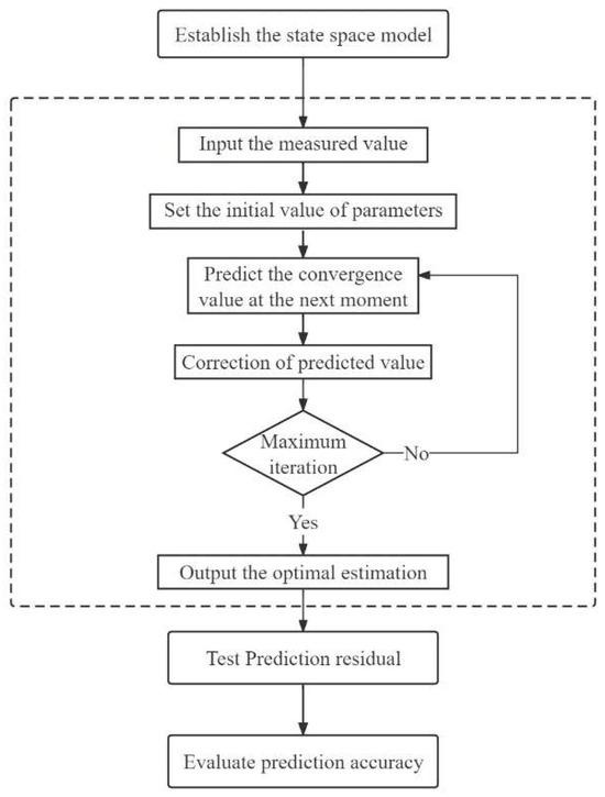
Figure 1.
The process of lateral convergence model development for subway shield tunnel based on the Kalman algorithm.
2.1. Prediction Model Based on Kalman Filtering Theory
Kalman filtering is an algorithm that utilizes the state equation of a linear system to optimally estimate the system state through the input and output observations of the system. The state space model constructed based on the Kalman filtering principle is as follows:
State equations:
Observation equations:
where is the state matrix of the system at moment K, A is the state transition matrix of the system, B is the control input matrix, is the control vector matrix at moment K, is the process noise matrix of the system at moment K, is the measurement value of the system at moment K, H is the state observation matrix, and is the measurement noise matrix of the system at moment K. The noise variables and conform to a Gaussian distribution with covariances of Q and R, respectively. For a system without external forces, the term in Equation (1) does not exist.
The advantage of the Kalman filtering method is its ability to eliminate the influence of a random disturbance error and obtain the data closest to the real situation [29]. It constantly adjusts the state according to the measured data during the operation process to improve accuracy. The horizontal diameter data of a subway shield tunnel have non-stationary, time-varying, and random characteristics. Iterating and adjusting the prediction model based on the measured values of horizontal diameter can allow the predicted values to be more accurate. Therefore, the prediction model based on the Kalman filtering principle shows outstanding performance in terms of predicting the lateral convergence deformation of a subway shield tunnel. The lateral convergence model of a subway shield tunnel based on the Kalman algorithm combines Bayes’ theorem and least squares estimation to estimate the system state in a recursive way. Bayes’ theorem states that the posterior probability is calculated using observed data under the condition of known prior probability. In the model, the prior probability is the initial estimate of the system state, and the posterior probability is the optimal estimate of the system state. Least squares estimation determines the parameters by minimizing the square error between the observed values and the estimated values. Least squares estimation is applied in the model to determine the relationship between the estimated value and the measured value of the system state and to update the estimated values of the system state. The prediction model based on the Kalman filtering theory first predicts the state of the present moment according to the predicted value of the previous moment, that is, the prior state estimation, and then revises the prior state estimation by using the measured value of the present moment to obtain the optimal state estimation (posterior state estimation). The Kalman model is divided into two parts: prediction and update. In the prediction step, the prior state predicted value is passed to the next moment through the state transition matrix, and then the system covariance matrix is updated. In the update step, the optimal estimation is obtained through weighted prior state estimation and measurements. The specific steps are as follows:
Predicting the state of the system at moment K:
Predicting the covariance matrix of the system at moment K:
Equations (3) and (4) are the prediction part of the model, the input values of which are the optimal estimation at moment K − 1, the optimal covariance matrix of the system, and the process noise covariance matrix, and the output values are the predicted value of the system at moment K and the predicted value of the system covariance matrix at moment K.
Calculating the Kalman gain:
Updating the system state at moment K:
Updating the covariance matrix of the system:
Equations (5)–(7) are the update part of the model, the input values of which are the output values of the prediction part, the measurement value of the system, the measurement noise covariance, and the state observation matrix, and the output values are the optimal estimation and covariance matrix modified by the measurement value.
In the above equations, represents the predicted value of the prior state, represents the optimal estimation of the state, represents the Kalman gain, represents the optimal covariance matrix of the system at moment K, and represents the predicted value of the covariance matrix of the system at moment K.
There are also some variables in the lateral convergence model of a subway shield tunnel based on the Kalman algorithm that play an important role in the effectiveness of the model.
R is the covariance of the measurement noise with a zero mean of the normal distribution, which represents the degree of trust in the measured value. The smaller the value of R, the higher the degree of trust in the measured value; the faster the model convergence rate, the larger the value of R, the lower the trust in the measured value, and the slower the model convergence rate. It is inappropriate for R to be too large or too small. If the R value is too small, there will be oscillatory behavior; if it is too large, the model convergence speed will be slow.
Q is the covariance of the process noise with a zero mean of the normal distribution, which represents the degree of trust in the model-predicted value. The smaller the value of Q, the higher the degree of trust in the model predicted value; the larger the value of Q, the lower the degree of trust in the model predicted value, and the higher the degree of trust in the measured value. A value of Q that is too small leads to system divergence.
The Kalman gain K refers to changes in the degree of uncertainty after each update of the model, quantified by the covariance of the variables. With each iteration of the model, if uncertainty decreases, the prediction results are more accurate and K plays a positive gain role. So, the Kalman gain is the core of the whole calculation process. In the process of model iteration, the prior estimation is modified by weighing the difference between the actual measured value and the prior estimation, and this weighting ratio is the Kalman gain. The convergence value of the Kalman gain is Q/(Q + R), and the larger the value of K, the more reliable the measured value; the smaller the K value, the more reliable the prediction.
The Kalman prediction model not only has a small amount of computation and fast running speed but it can also adjust the predicted value constantly according to the measured data, and it can adapt well to different environments and noise conditions. In addition, the model estimates the system state in a recursive way, which can reduce the impact of system noise and interference, ensuring the accuracy and robustness of the model. All in all, the Kalman prediction model has the advantages of high efficiency, self-adaptability, and high robustness, which are suitable for the lateral convergence deformation prediction of subway shield tunnels.
2.2. Parameter Setting
For the one-dimensional lateral convergence model of a subway shield tunnel based on the Kalman algorithm, the process of setting the initial parameters is as follows:
H = [1], where H represents the state transition relationship between X and Z values. Since X and Z represent the horizontal diameter of the subway shield tunnel, which is a metric value of the same scale, the state observation matrix is set to [1].
A = [1], where A represents the state transition relationship between multiple X values. The horizontal diameter of the subway shield tunnel does not show a unidirectional decline trend. The artificial adjustment of the A value will cause the model deviation to become increasingly larger over time, so A is set as a first-order unit matrix.
R = 0.01, where the instrument used for the data collection is the German Z + F 6012 series scanner, and the measurement accuracy of its section point is 10 mm; it needs to be consistent with the unit of the horizontal diameter measurement value of subway shield tunnel m, so the measurement noise is set to 0.01.
Q = , where Q takes the variance of the horizontal diameter measured value of a subway shield tunnel, and the variance is given by , where is the population variance, X is the variable, μ is the population mean, and N is the number of population cases. In the actual calculation, sample statistics are used to replace the population parameter. Sample variance is given by , where is the sample variance, X is the variable, is the sample mean, and n is the number of sample cases. The process noise Q of this lateral convergence model of a subway shield tunnel based on the Kalman algorithm is obtained by taking the variance of the subway shield tunnel horizontal diameter measurement Z.
P = [1], where the initial value of P is the covariance of the system at the initial moment, which affects the convergence speed at the initial moment and has little impact on the overall convergence effect on the horizontal diameter of a subway shield tunnel. It can be set to 1, and then P will be iterated continuously according to the change in the Kalman gain and will converge to the optimal estimated covariance matrix.
2.3. Evaluation Criteria
2.3.1. Prediction Residual Tests
The residual is the difference between the actual observed value and the fitted value, reflecting the portion of the dependent variable that is not explained by the independent variable. According to the central limit theorem, the mean values of a large number of mutually independent random variables tend to be normally distributed under certain conditions. The fact that the residuals conform to a normal distribution indicates that the residuals are random variables, and that the model has a good fit to random errors, which proves that the model has a high degree of fit and a strong prediction ability. Normality tests, skewness–kurtosis tests, and graphical tests are commonly used to test whether the residuals follow a normal distribution.
The normality test methods are the Shapiro–Wilk test and Kolmogorov–Smirnov test. The S–W test is suitable for a sample size of less than 50 small-sample tests, and the K–S test is suitable for a sample size of more than 50 large-sample tests. The original hypothesis of the normality test is as follows: “If the population from which the sample comes has no significant difference from the normal distribution, it conforms to the normal distribution”. If the significance of the p-value is less than 0.05, the original hypothesis is rejected, indicating that the data do not conform to a normal distribution; on the contrary, if the level is not significant, the original hypothesis is accepted, and the data conform to normal distribution.
Skewness describes the skewness degree and direction of the data distribution. If skewness is greater than 0, the tail on the right side of the curve is longer, the data on the left side are denser, the distribution is skewed to the right, and the mean > median > mode; when skewness is less than 0, the tail on the left side of the curve is longer, the data on the right side are denser, the distribution is skewed to the left, and the mode > median > mean. The larger the absolute value of skewness, the more skewed the data distribution is. Kurtosis is a statistic that studies the degree of steepness and flatness of the data distribution curve. If kurtosis is greater than 0, the data distribution is steeper than the peak state of the standard normal distribution; if kurtosis is less than 0, the data distribution is flatter than the peak state of the standard normal distribution. The skewness and kurtosis of the standard normal distribution are both 0. For the actual sample data, we generally believe that if the absolute value of kurtosis is less than 10 and the absolute value of the skewness is less than 3, then it can be basically accepted as a normal distribution [30].
The graphical tests include a histogram, P-P plot, and Q-Q plot. If the histogram presents a “bell-shaped plot with a high center and low sides, and basic symmetry between the left and the right”, the data follow a normal distribution. The probability–probability plot is a graph based on the relationship between the cumulative proportion of variables and the cumulative proportion of the specified distribution, which tests whether the data conform to the specified distribution. When the data conform to the normal distribution, the points in the plot are approximately a straight line. The quantile–quantile plot is a graphical comparison of the probability distribution of two probability distributions in different quantiles. When it is used to test whether the data conform to the normal distribution law, the sample data are taken as the X-axis, and the expected quantile of the normal value data is taken as the Y-axis, in order to generate the scatter plot. The higher the coincidence degree between the scatter point and the straight line, the more the sample data follow a normal distribution.
2.3.2. Comparison of Prediction Accuracy
At present, there are many methods that are used to measure prediction accuracy, and the following types of measurement methods are mainly used for the assessment of univariate time series data: scale-dependent measurements, percentage error-based measurements, and relative error-based measurements [31]. Scale-dependent measurements are usually based on absolute error or square error, and the commonly used indicators include mean square error (MSE), root mean square error (RMSE), mean absolute error (MAE), median absolute error (MedAE), and so on. Measurements based on percentage error are dependent on the data scale, and the commonly used indicators include the mean absolute percentage error (MAPE), median absolute percentage error (MedAPE), root mean square percentage error (RMSPE), etc. Relative error-based measurements need to be compared with the errors obtained by standard prediction methods, represented by indicators such as mean relative absolute error (MRAE) and median relative absolute error (MedRAE), as well as others.
Considering the advantages and disadvantages of the above indicators, we decided to use the RMSE, NRMSE, MAPE, and R2 in this paper to measure the prediction accuracy of the model. RMSE is an indicator used to measure the difference between the predicted value and the measured value of the model, which can better evaluate the degree of fit of the model and can be used to measure the accuracy of the same set of data using different prediction models. The NRMSE is a normalized RMSE that overcomes scale dependence and is used to measure the difference between predicted and measured values relative to the range of measured values. The MAPE shows the relative magnitude of deviation of the model prediction value in the form of a percentage, which has the advantage of being independent of data scale; therefore, it can be used to judge the prediction performance of different datasets. R2 characterizes the degree to which the model can explain changes in the dependent variable, and it is used to evaluate the model’s fit to the measured values.
where is the measured value, is the predicted value, is the mean of the measured values, and n is the number of measured values.
3. Case Analysis
3.1. Project Overview and Testing Data
The data in this paper are selected from the two-station section of a subway tunnel. The designed mileage of the section tunnel is DK12+043.600~DK12+618.236, among which the length of the left line tunnel is 526.356 m, and the length of the right line tunnel is 538.301 m. The project was completed and began operations in 2013. The maximum buried depth of the interval tunnel is 19.04 m, the minimum buried depth is 8.16 m, and the tunnel passes through a large number of residential houses, mostly 1–8-story buildings. The interval is constructed by the shield method. The inner diameter of the tunnel is 5.4 m, the outer diameter is 6 m, and the width of the shield segment is 1.5 m.
The horizontal diameter value of the tunnel is used to characterize the lateral convergence deformation of the subway shield tunnel during operation (Figure 2). A mobile 3D laser scanner, called Amberg GRP5000 (Amberg Technologies, Zurich, Switzerland), was used to collect nine sets of point cloud data of subway shield tunnels in August 2018, February 2019, November 2019, June 2020, November 2020, May 2021, November 2021, March 2022, and September 2022. The point cloud data were projected onto a horizontal plane to obtain the tunnel boundary point cloud, which is the left and right endpoints of the tunnel horizontal diameter, thus obtaining the horizontal diameter of the subway shield tunnel ring by ring. The total of the horizontal diameter values of the 200-ring segments of the tunnel was extracted. By utilizing the horizontal diameter data of multi-ring subway shield tunnels, the lateral convergence deformation prediction accuracy of a subway shield tunnel based on the Kalman model can be fully verified. The performance of the Kalman model in predicting the lateral convergence deformation of a subway shield tunnel using datasets of different scales can also be analyzed by inputting sample data from different periods.
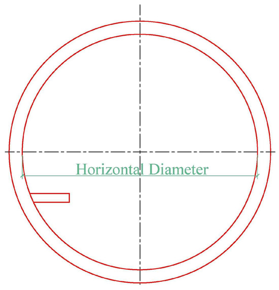
Figure 2.
Schematic diagram of horizontal diameter of tunnel.
For the shield tunnel with staggered splicing, the early warning value and safety value of convergence deformation are specified in the Specifications for Operational Monitoring of Urban Rail Transit Facilities (GB/T39559.3-2020) [32]. The early warning indicator is 7.2‰ of the tunnel outer diameter, and the safety indicator is 9‰ of the tunnel outer diameter. The over-limit of the convergence deformation value will affect the traffic safety of the tunnel. Taking the data from September 2022 as an example, there are 43 rings of 200-ring tubes where the horizontal diameter reaches the warning limit, 31 rings in which the horizontal diameter exceeds the safety limit, and the rest of them meet the standard requirements, as shown in Figure 3.
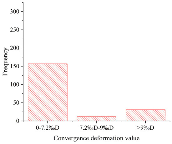
Figure 3.
The convergence deformation value distribution of the horizontal diameter of a 200-ring shield tunnel segment.
3.2. Lateral Convergence Model of Subway Shield Tunnel Based on Kalman Algorithm
According to Formulas (3)–(7) in Section 2.1, we establish a lateral convergence model for the Kalman subway shield tunnel on the MATLAB platform, input the horizontal diameter of the tunnel as the observation value, and set the initial parameters described in Section 2.2. In this model, the horizontal diameter values of the ninth phase of the tunnel correspond to K = 1–9 time points, respectively. First, based on the observation values and initial parameters at time K = 1, the predicted horizontal diameter and covariance matrix at time K = 2 are calculated. Then, the Kalman gain at time K = 2 is calculated, and the predicted horizontal diameter at time K = 2 is corrected based on the Kalman gain and observation values at time K = 2. The optimal estimate of the horizontal diameter at time K = 2 and the corrected covariance matrix are obtained. The optimal estimate of the horizontal diameter at time K = 2 and the corrected covariance matrix are used to predict the horizontal diameter at time K = 3. Then, the Kalman gain at time K = 3 is calculated, and the horizontal diameter prediction at time K = 3 is corrected based on the Kalman gain and the observed values at time K = 3. The optimal estimate of the horizontal diameter at time K = 3 and the corrected covariance matrix are obtained. By obtaining these, we can iterate through the entire dataset and output the final optimal estimate of the horizontal diameter.
Taking one of the segments as an example, the horizontal diameter value of the tunnel is Z = [5.431, 5.429, 5.43, 5.427, 5.424, 5.428, 5.428, 5.427, 5.4267]. The first eight Z-values are inputted into the Kalman model as observation values to predict the horizontal diameter value of the tunnel at time K = 9 and are compared with the Z-value of the ninth period, 5.4267, to test the accuracy of the model. The predicted results are shown in Figure 4, where a black * represents the measured values of the first eight phases of the tunnel horizontal diameter, a red * represents the measured values of the ninth phase of the tunnel horizontal diameter, and the blue dashed line represents the iterative process of the predicted values of the horizontal diameter. From the figure, it can be seen that the predicted horizontal diameter values closely match the measured values with minimal error. The predicted value will continuously adjust with the fluctuation in the measured value, and the trend in the two changes is basically consistent, indicating that the fit of the model is good. The predicted value of the horizontal diameter in the ninth period is 5.4276 m, while the measured value in the ninth phase is 5.4267 m, with a prediction residual of 0.0009 m, which is 0.9 mm. The error is very small, and the prediction accuracy is high.
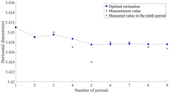
Figure 4.
Kalman model single-ring segment prediction results.
The Kalman gain is an important parameter in the model, and its variation has a significant impact on the performance of the prediction model. For example, the Kalman gains in the prediction process of the horizontal diameter value of the abovementioned pipe segments are [0.9901, 0.4976, 0.3325, 0.2498, 0.2002, 0.1671, 0.1435]. At the initial moment, the Kalman gain is large, indicating that the measured values have a significant impact on the system. As time increases, the Kalman gain gradually decreases, indicating that the confidence of the predicted values gradually increases, the dependence on the measured values decreases, and the impact of the predicted values on the system becomes increasingly significant. The final Kalman gain is about 0.14, which is relatively small, indicating that the system is relatively stable and mainly depends on the predicted value.
In addition, the absolute error of the predicted value obtained through calculation is 8.7487 × 10⁻⁴, and the percentage error is 0.0161. The absolute error reflects the absolute value of the difference between the predicted value and the measured value. The smaller the absolute error, the smaller the difference between the predicted value and the measured value, and the higher the prediction accuracy. The percentage error is the ratio of the difference between the predicted value and the measured value to the measured value, reflecting the relative error of the predicted value relative to the measured value. The smaller the percentage error, the higher the prediction accuracy. It can be seen that the Kalman subway shield tunnel lateral convergence model shows high accuracy and high precision and can provide reliable prediction results.
All the collected horizontal diameter values of the 200-ring segment are predicted by the lateral convergence model of a subway shield tunnel based on the Kalman algorithm, and the overall root mean square error RMSE = 8.2990 × 10⁻⁴, the normalized root mean square error NRMSE = 0.0097, the mean absolute percentage error MAPE = 0.0124, and the coefficient of determination R2 = 0.9979 were calculated. The smaller values of RMSE and NRMSE indicate a smaller difference between the predicted and measured values of the model, indicating a higher prediction accuracy of the model. A small MAPE indicates that the average prediction error of the model is small, and the prediction accuracy of the model is high. The R2 value ranges between 0 and 1, with 0.9979 being very close to 1, indicating that the model fits well with the measured data. The optimal estimation values output by the prediction model were compared with the measured value. Figure 5 shows the comparison between the predicted value and the measured value of the Kalman model, and Figure 6 shows the prediction residual of the Kalman model. The predicted value of the horizontal diameter of the 200-ring pipe segment is highly consistent with the measured value, indicating the high accuracy of the model. In summary, combined with the image and the precision measurement indicator, it can be seen that the predicted value and measured value of the Kalman prediction model have a high degree of fit, and the residual value is small; the prediction effect is great when this applies to multi-ring segments.
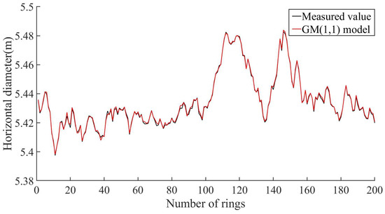
Figure 5.
Comparison of the predicted value and measured value of Kalman model multi-ring segments.
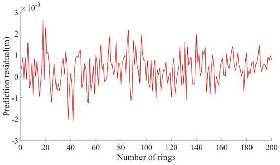
Figure 6.
Prediction residual of the Kalman model multi-ring segments.
The lateral convergence deformation prediction residual of a subway shield tunnel based on the Kalman model is analyzed below to test whether it conforms to a normal distribution. According to the histogram of residual distribution predicted by the Kalman model (Figure 7), there are 162 rings of its residuals which are in the range of [−0.001, 0.001] m, 33 rings in the range of [−0.002, 0.001] ∪ [0.002, 0.001] m, 33 rings in the range of [−0.002, 0.001] m, and only 5 rings in the range of [−0.003, −0.002] ∪ [0.003, 0.002] m; the histogram presents with a bell-shaped plot with a high center and low sides. Through the K–S test of a large sample size, p = 0.057 > 0.05 is obtained, which proves that the residuals conformed to normal distribution, so the Kalman prediction model has a high degree of fit and a strong prediction ability. The normality test results of the data are shown in Table 1. The normal distribution skewness of the residual is −0.128, which is less than 0, the tail on the left side of the curve is longer, and the data on the right side are denser, indicating that the normal distribution is skewed to the left; the kurtosis of the residual is 0.498, which is greater than 0, indicating that the peak state of the normal distribution is steeper. The mean value of the residual normal distribution is positive, indicating that the lateral convergence deformation prediction value of a subway shield tunnel based on the Kalman model is larger than the measured value.
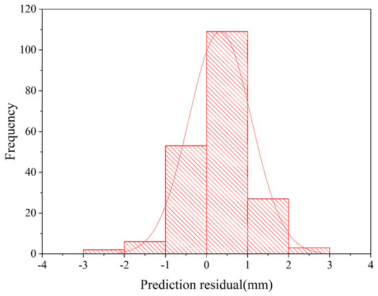
Figure 7.
Kalman model prediction residual distribution histogram (200-ring segment).

Table 1.
Normality test results of predicted residual.
In addition, the sample points in the normal P-P plot and Q-Q plot of the predicted residual (Figure 8 and Figure 9) are approximately a straight line, which also proves that they follow a normal distribution.
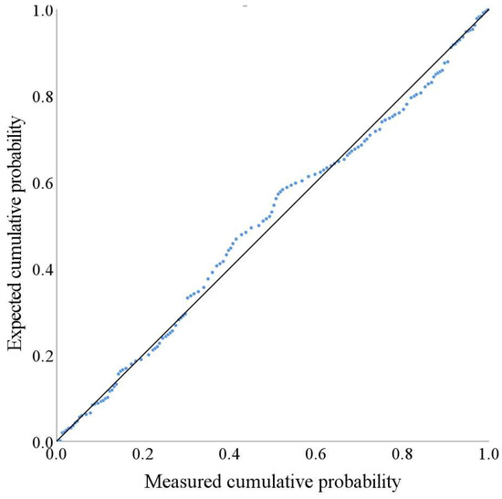
Figure 8.
Normal P-P plot of predicted residual.
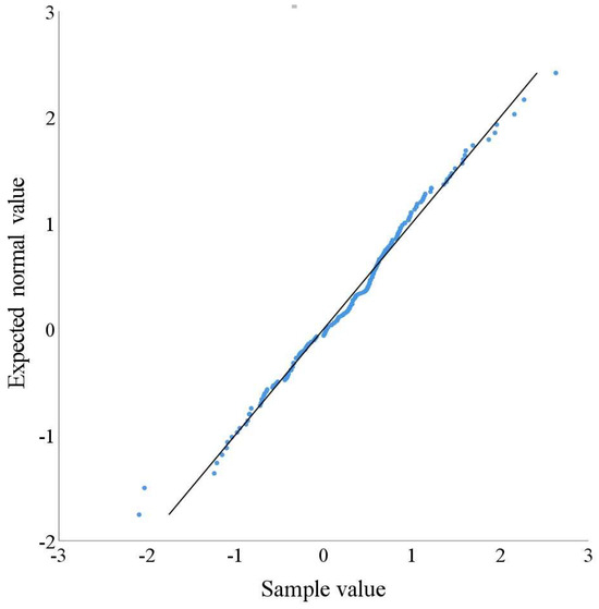
Figure 9.
Normal Q-Q plot of predicted residual.
4. Discussion
4.1. Comparison of Prediction Accuracy of Multiple Models
In order to further measure the lateral convergence deformation prediction accuracy of a subway shield tunnel based on the Kalman model, we make a comparison between the GM(1,1) model and the GM–Markov model.
The GM(1,1) model refers to the grey model of a single-variable first-order differential equation, which is the most widely used form of grey prediction. Its prediction principle is to change the original data without obvious regularity into a series with an exponential growth pattern through accumulated generating and to construct a series of equal weights adjacent to the mean value of the accumulated generated sequence to eliminate the volatility and randomness of the original data. Since the form of the solution of the first-order differential equation is exponential growth, the first-order differential equation model can be established for the sequence of the equal weights of the adjacent mean. After that, the development coefficient and grey action are solved by the least square method and substituted into the first-order differential equation, and the data are reversely calculated; cumulative reduction is then carried out to obtain the prediction value of the original sequence. The model adopts the method of accumulation and reduction, which does not need to find the statistical regular pattern of the original series but rather directly converts it into a regular time series, weakens the unknown factors in the grey system, strengthens the influence degree of known factors, and is suitable for the short-term prediction of a small-sized sample of data.
For the data showing volatility and trend, the Markov chain is introduced to improve the fit of the grey model. The Markov chain is characterized by the fact that the future state of the system is only related to the present state and has nothing to do with the past state, and the state transition has no after-effect. The GM–Markov model is used to obtain the prediction value of the original data by using the GM(1,1) model, and then the GM(1,1) model is established using the residual difference between the original data and the prediction value in order to obtain the residual correction value. The positive and negative residuals are divided into two states, and the probability of each state transferring to each other is obtained based on the sample data; then, the state transition matrix is constructed, and the state probability of the final moment is obtained. The state with the greatest probability is selected as the final state, and the residual correction value in this state is used to correct the original data prediction value and accurately adjust the prediction result.
Figure 10 shows the comparison of the prediction results for the GM(1,1) model, the GM–Markov model, and the Kalman model for a single-ring segment. It can be seen from the figure that the prediction result of the GM(1,1) model is a straight line, and the fitting effect of the volatility data is poor. However, the GM–Markov model is adjusted on the basis of the GM(1,1) model prediction curve, the predicted result is closer to the actual measured value than that of the GM(1,1) model in later periods, and the prediction effect is better. Among the three models, the curve trend of the Kalman model is the closest to the measured value, and the prediction effect is the best. Table 2 shows the calculation results of the absolute error and percentage error for the predicted values of the three kinds of models for the single-ring segment. The absolute error and percentage error of the Kalman model are smaller than those of the other two kinds of models, indicating that the Kalman model has higher prediction accuracy and more reliable prediction results.
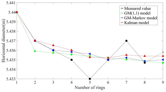
Figure 10.
Prediction results comparison of three kinds of models (single-ring segment).
Table 2.
Absolute error and percentage error of predicted values for single-ring pipe segments using three models.
The prediction results of the GM(1,1) model, the GM–Markov model, and the Kalman model for the 200-ring segment of a shield tunnel are shown in Figure 11. For the convenience of observation and analysis, 40 consecutive ring segments are captured and plotted (Figure 12). The predicted value and residual value of each ring segment are shown in Table 3. It can be seen from Figure 10 that the red line representing the Kalman prediction model is closer to the black line representing the measured value than the green line and blue line representing the GM(1,1) prediction model and the GM–Markov prediction model, respectively, indicating that the prediction effect of the Kalman model is better in the case of multi-ring segments, which proves the generality of the Kalman model.
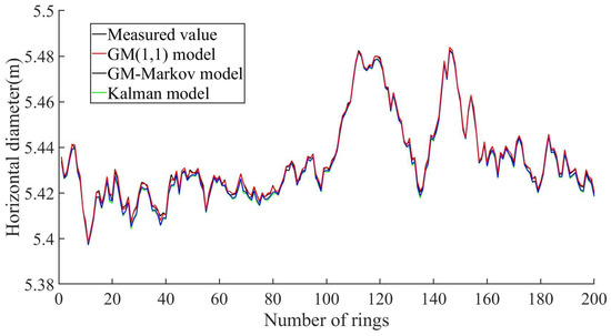
Figure 11.
Comparison of the predicted values and measured values of the three kinds of models (200-ring segment).
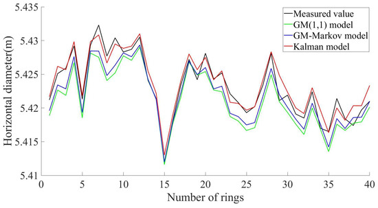
Figure 12.
Comparison of the predicted values and measured values of the three kinds of models (40-ring segment).
Table 3.
The predicted value and residual value of three kinds of models (40-ring segment).
Figure 13 shows the residuals of the prediction results of the three kinds of models for the 200-ring segment. The residuals of the Kalman model are mostly concentrated in the interval of [−0.001, 0.001] m, and the residuals are small, indicating that the Kalman model is stable and has a good prediction effect. The residuals of the GM(1,1) model are distributed in the interval of [−0.005, 0.002] m, and the residuals of some prediction results are more significant, indicating that the prediction result of the GM(1,1) model is unstable and that the prediction effect is general. The residuals of the GM–Markov model are mainly concentrated in the interval of [−0.003, 0.002] m, and a few prediction residuals can reach −0.005 m. The prediction effect is better than the GM(1,1) model but inferior to the Kalman model. In addition, the residuals of the GM(1,1) model and the GM–Markov model are mostly negative, which indicates that the prediction results of the GM(1,1) model and the GM–Markov model are smaller than the measured value.
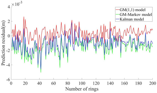
Figure 13.
Comparison of prediction residuals of three kinds of models (200-ring segment).
The GM(1,1) model, GM–Markov model, and Kalman model were used to predict the horizontal diameter of the 200-ring segment, and the overall root mean square error (RMSE), normalized root mean square error (NRMSE), the mean absolute percentage error (MAPE), and coefficient of determination R2 are shown in Table 4. The RMSE, NRMSE, and MAPE values of the Kalman model are all smaller than the other two models, indicating that the Kalman model has more accurate prediction results and a higher prediction accuracy. The R2 of the Kalman model is closer to one than the other two models, indicating that the Kalman model fits the data better. Taking into account various indicators, it is proven that the Kalman model has a higher prediction accuracy.
Table 4.
RMSE, NRMSE, MAPE, and R2 of the three kinds of models (200-ring segment).
4.2. Prediction Performance of Kalman Model in Different Scale Datasets
In order to measure the lateral convergence deformation prediction performance of a subway shield tunnel based on the Kalman model on datasets with different scales, the horizontal diameter convergence data of a shield tunnel in the 1–4, 1–5, 1–6, 1–7, and 1–8 periods of a 200-ring segment were selected as sample data to predict the convergence value of the tunnel horizontal diameter for the 5th, 6th, 7th, 8th, and 9th periods, respectively. Figure 14 shows the RMSE, NRMSE, MAPE, and R2 values of different scale datasets. When only four periods of data were used as sample data for prediction, the root mean square error RMSE = 0.0037 increased by 131% compared with the five periods of data, the mean absolute percentage error MAPE = 0.0656 increased by 185% compared with the five periods of data, and the normalized root mean square error NRMSE = 0.0432 increased by 136% compared with the five periods of data. In this scenario, the coefficient of determination R2 is 0.9596, while the R2 for the 5–9 period of data is close to 1. This indicates that the prediction effect of the four periods of data was not good. There should be at least five periods of data to use the Kalman model to predict the convergence value of the tunnel horizontal diameter. As the number of periods of sample data increases, the RMSE, NRMSE, and MAPE values of the Kalman model gradually decrease, and R2 approaches 1, indicating that the prediction accuracy of the model will be improved with an increase in sample data.
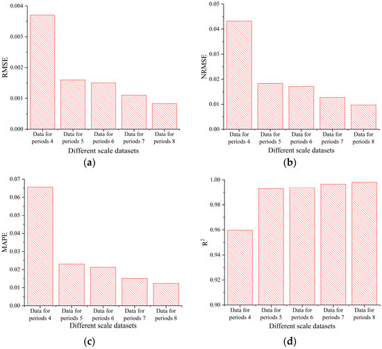
Figure 14.
Prediction performance in different scale datasets: (a) RMSE, (b) NRMSE, (c) MAPE, (d) R2.
5. Conclusions
In this paper, the Kalman model is used to predict the lateral convergence deformation of a subway shield tunnel, and the main conclusions are as follows:
- The lateral convergence model of a subway shield tunnel based on the Kalman algorithm performs well in the prediction of non-stationary data with a small sample size. This model is efficient, adaptive, and robust and can accurately predict the lateral convergence deformation of a subway shield tunnel.
- For the prediction of the horizontal diameter data of a subway shield tunnel, comparing the Kalman model with the GM(1,1) model and the GM–Markov model, it is found that the lateral convergence model of a subway shield tunnel based on the Kalman algorithm has a high degree of fit with the horizontal diameter measured value; additionally, the prediction residual is small, and the model effect is better. The RMSE, NRMSE, MAPE, and R2 are introduced as evaluation indicators to verify the lateral convergence deformation prediction accuracy of a subway shield tunnel based on the Kalman model.
- By observing the performance of the Kalman model in predicting the lateral convergence deformation of a subway shield tunnel using datasets of different scales, it is found that at least five periods of horizontal diameter sample data of subway shield tunnels are required for predicting the lateral convergence deformation of a subway shield tunnel, and the prediction accuracy of the model improves with the increase in the number of sample data periods. As the number of horizontal diameter sample data periods of subway shield tunnels increases, the lateral convergence deformation prediction accuracy of a subway shield tunnel based on the Kalman model is improved.
There are some shortcomings in the research process. For example, if the sample size of the validation model is limited, tunnel convergence deformation data under different environmental and geological conditions should be used for validation to increase the generalization performance of the Kalman model. This article proves through comparison that the Kalman model has a higher accuracy than the GM (1,1) model and the GM Markov model. However, there are currently other models that can be applied to predict tunnel convergence deformation, and future research should consider a wider range of model comparisons. In addition, we also consider incorporating the Kalman prediction model into tunnel intelligent operation and maintenance systems to reduce tunnel maintenance costs, improve the safety of tunnel operations, and assist in the sustainable development of tunnels.
Author Contributions
Conceptualization, Y.Z.; methodology, Y.Z.; software, Y.Z. and D.Z.; validation, Y.Z. and Y.B.; formal analysis, Y.Z.; investigation, Y.Z., D.Z. and L.W.; resources, C.T., Y.B. and L.W.; data curation, C.T., Y.B. and L.W.; writing—original draft preparation, Y.Z.; writing—review and editing, X.M., Y.B. and Z.S.; visualization, Y.Z.; supervision, X.M., Y.B., Z.S. and C.T.; project administration, Y.Z., D.Z. and L.W.; funding acquisition, Y.B. All authors have read and agreed to the published version of the manuscript.
Funding
This research was funded by the National Natural Science Foundation of China, grant numbers 51829801 and 52378385.
Institutional Review Board Statement
Not applicable.
Informed Consent Statement
Not applicable.
Data Availability Statement
The data presented in this study are available on request from the corresponding author.
Conflicts of Interest
Author Chao Tang was employed by the company Beijing Urban Construction Exploration & Surveying Design Research Institute Co., Ltd. The remaining authors declare that the research was conducted in the absence of any commercial or financial relationships that could be construed as a potential conflict of interest.
References
- Huang, H.; Xue, Y.; Shao, H.; Du, J. Rapid Detection and Engineering Practice of Urban Subway Shield Tunnel Disease; Shanghai Scientific Technical Publishers: Shanghai, China, 2018. [Google Scholar]
- Tian, N.; Chen, J.; Lu, Y. Influence of Ground Surface Surcharge on Deformational Behavior of Existing Tunnel Based on 3D Random Field. In Proceedings of the Geo-Risk 2023, Arlington, Virginia, 23–26 July 2023; pp. 33–43. [Google Scholar]
- Mu, B.; Xie, X.; Li, X.; Li, J.; Shao, C.; Zhao, J. Monitoring, modelling and prediction of segmental lining deformation and ground settlement of an EPB tunnel in different soils. Tunn. Undergr. Space Technol. 2021, 113, 103870. [Google Scholar] [CrossRef]
- Sharifzadeh, M.; Tarifard, A.; Moridi, M.A. Time-dependent behavior of tunnel lining in weak rock mass based on displacement back analysis method. Tunn. Undergr. Space Technol. 2013, 38, 348–356. [Google Scholar] [CrossRef]
- Debernardi, D.; Barla, G. New Viscoplastic Model for Design Analysis of Tunnels in Squeezing Conditions. Rock Mech. Rock Eng. 2009, 42, 259–288. [Google Scholar] [CrossRef]
- Tan, Y.; Chen, B.; Liu, Z. Study on Large Deformation Characteristics and Secondary Lining Supporting Time of Tunnels in Carbonaceous Schist Stratum under High Geo-Stress. Sustainability 2023, 15, 14278. [Google Scholar] [CrossRef]
- Satici, Ö.; Topal, T. Assessment of damage zone thickness and wall convergence for tunnels excavated in strain-softening rock masses. Tunn. Undergr. Space Technol. 2021, 108, 103722. [Google Scholar] [CrossRef]
- Li, H.; Li, X.; Yang, Y.; Liu, Y.; Ma, M. Structural Stress Characteristics and Joint Deformation of Shield Tunnels Crossing Active Faults. Appl. Sci. 2022, 12, 3229. [Google Scholar] [CrossRef]
- Deng, P.; Liu, Q.; Liu, B.; Lu, H. Failure mechanism and deformation prediction of soft rock tunnels based on a combined finite–discrete element numerical method. Comput. Geotech. 2023, 161, 105622. [Google Scholar] [CrossRef]
- Yi, Z. Research on Operation Resilience Assessment of Subway Tunnel System Based on Dynamic Bayesian Network (DBN). Master’s Thesis, Huazhong University of Science and Technology, Wuhan, China, 2020. [Google Scholar]
- Huang, H.-W.; Zhang, Y.-J.; Zhang, D.-M.; Ayyub, B.M. Field data-based probabilistic assessment on degradation of deformational performance for shield tunnel in soft clay. Tunn. Undergr. Space Technol. 2017, 67, 107–119. [Google Scholar] [CrossRef]
- Ai, Q.; Peng, Z.; Lang, Q.; Su, D.; Peng, C.; Chi, Y.; Zhu, J.; Jiang, Z.; Tang, H.; Luo, R. A Dynamic Early Warning Method for Abnormal Data in Tunnel Health Monitoring Based on ARIMA Model. CN116163807A, 15 December 2022. [Google Scholar]
- Zhang, H.; Wu, Y.; Yang, S. Probabilistic analysis of tunnel convergence in spatially variable soil based on Gaussian process regression. Eng. Appl. Artif. Intell. 2024, 131, 107840. [Google Scholar] [CrossRef]
- Mahmoodzadeh, A.; Taghizadeh, M.; Mohammed, A.H.; Ibrahim, H.H.; Samadi, H.; Mohammadi, M.; Rashidi, S. Tunnel wall convergence prediction using optimized LSTM deep neural network. Geomech. Eng. 2022, 31, 545–556. [Google Scholar]
- Ma, T.; Jin, Y.; Liu, Z.; Prasad, Y.K. Research on Prediction of TBM Performance of Deep-Buried Tunnel Based on Machine Learning. Appl. Sci. 2022, 12, 6599. [Google Scholar] [CrossRef]
- Torabi-Kaveh, M.; Sarshari, B. Predicting Convergence Rate of Namaklan Twin Tunnels Using Machine Learning Methods. Arab. J. Sci. Eng. 2019, 45, 3761–3780. [Google Scholar] [CrossRef]
- Ning, W.; Zhou, L.; Ning, Y.; Yang, B. Construction and correction of prediction model in tunnel deformation monitoring. J. Southeast Univ. (Nat. Sci. Ed.) 2013, 43 (Suppl. S2), 279–282. [Google Scholar]
- Bi, W.; Tian, G.; Zhang, Y.; Yang, S.; Kong, X. Discussion on Using Grey Theory to Predict Tunnel Deformation. Mod. Tunn. Technol. 2011, 48, 53–57. [Google Scholar]
- Xia, C.; Bian, Y.; Jin, L. A Comparison between Grey and Regression Model for Tunnel Deformation Prediction. West. China Commun. Sci. Technol. 2010, 1, 5–8+13. [Google Scholar]
- Fei, J.; Wu, Z.; Sun, X.; Su, D.; Bao, X. Research on tunnel engineering monitoring technology based on BPNN neural network and MARS machine learning regression algorithm. Neural Comput. Appl. 2020, 33, 239–255. [Google Scholar] [CrossRef]
- Zhou, J.; Chen, Y.; Li, C.; Qiu, Y.; Huang, S.; Tao, M. Machine learning models to predict the tunnel wall convergence. Transp. Geotech. 2023, 41, 101022. [Google Scholar] [CrossRef]
- Li, Q.; Jiang, W.; Tang, C.; Xu, H. Analysis and prediction on the structure deformation of cross river shield tunnel. Bull. Surv. Mapp. 2022, 9, 34–38. [Google Scholar]
- Lu, B.; Pin, X.; Lu, R. Prediction of Convergent Deformation of Tunnel Surrounding Rocks Based on Grey Combination Model. J. Univ. Jinan (Sci. Technol.) 2022, 36, 689–695. [Google Scholar]
- Kalman, R.E. A New Approach to Linear Filtering and Prediction Problems. Trans. ASME J. Basic Eng. 1960, 82, 34–45. [Google Scholar] [CrossRef]
- Zhang, X.W.; Shang, J.Q.; Zhang, Q. Application of Kalman Filter Algorithm in Track Prediction. In Proceedings of the 5th International Conference on Information Science, Computer Technology and Transportation (ISCTT), Shenyang, China, 13–15 November 2020; IEEE: Shenyang, China, 2020; pp. 292–296. [Google Scholar]
- Yong, E.; Qian, W.; He, K. Penetration Ability Analysis for Glide Reentry Trajectory Based Radar Track. J. Astronaut. 2012, 33, 1370–1376. [Google Scholar]
- Wang, E.; Zhu, F.; Xiao, Y.; Tong, X.; Zhu, D. Generating Method of Adaptive Linear Signal Based on Kalman Prediction. Mod. Def. Technol. 2012, 40, 138–142. [Google Scholar]
- Xie, H.; Zhang, T. Application of Kalman Filter in Predicting High Frequency Financial Time Series Models. Stat. Decis. 2017, 13, 82–84. [Google Scholar]
- Cu, X.; Yu, Z.; Tao, B. Generalized Measurement Adjustment; Wuhan University Press: Wuhan, China, 2005. [Google Scholar]
- Kline, R.B. Principles and Practice of Structural Equation Modeling; The Guilford Press: New York, NY, USA, 2011. [Google Scholar]
- Hyndman, R.J.; Koehler, A.B. Another look at measures of forecast accuracy. Int. J. Forecast. 2006, 22, 679–688. [Google Scholar] [CrossRef]
- GB/T39559.3-2020; Specifications for Operational Monitoring of Urban Rail Transit Facilities. State Administration for Market Regulation, Standardization Administration of the People’s Republic of China: Beijing, China, 2020.
Disclaimer/Publisher’s Note: The statements, opinions and data contained in all publications are solely those of the individual author(s) and contributor(s) and not of MDPI and/or the editor(s). MDPI and/or the editor(s) disclaim responsibility for any injury to people or property resulting from any ideas, methods, instructions or products referred to in the content. |
© 2024 by the authors. Licensee MDPI, Basel, Switzerland. This article is an open access article distributed under the terms and conditions of the Creative Commons Attribution (CC BY) license (https://creativecommons.org/licenses/by/4.0/).