Are Natural Resource Rents and Renewable Energy Consumption Solutions for Environmental Degradation? Fresh Insights from a Modified Ecological Footprint Model

Abstract

A comprehensive approach addressing the key factors exacerbating pressure on the environment is required to minimize the damages caused by global warming and environmental destruction. For this purpose, the present study investigates the effects of renewable energy consumption (REC) and natural resource rents (NRRs) on environmental degradation within the scope of the environmental Kuznets curve (EKC) hypothesis for ASEAN-5 countries. Differing from most previous studies, this research represents environmental degradation by using the ecological footprint pressure index, which considers both the supply and demand aspects of the environment. The present study covers the period between 1990 and 2018. This study employs the Method of Moments Quantile Regression (MMQR), an advanced panel technique that yields reliable results on the outlier issue, endogeneity, and non-normal distribution. The MMQR results confirm the EKC hypothesis, assuming the presence of an inverted U-shaped relationship between economic growth and environmental degradation. Moreover, the results reveal that REC and NRRs reduce environmental degradation in all quantiles. Given these results, policymakers in the ASEAN-5 countries are recommended to utilize productivity gains from natural resource rents for investment in clean energy and to shift their energy consumption policies towards renewable energy technologies and research.

1. Introduction

In the modern era, natural resources are recognized as critical indicators that significantly contribute to reducing environmental pressure and increasing economic growth. However, as the global economy gains momentum and efforts for development intensify, the world increasingly faces the escalating cost of environmental degradation. Furthermore, the growing uncertainty surrounding non-renewable energy sources, coupled with the dimensions of climate change and environmental degradation, underscores the urgent necessity of transitioning to clean energy. Rapid economic growth and industrialization efforts significantly increase global warming and environmental degradation. Within this context, the recent changes in economic, social, and political structures in some countries and regions have reached levels threatening environmental sustainability [1,2]. The Association of Southeast Asian Nations (ASEAN) is one of the economic blocs established in 1967 with the objective of improving cooperation in various fields such as politics, economics, energy, security, and technology in the region. ASEAN-5, which is a group consisting of Indonesia, Malaysia, the Philippines, Singapore, and Thailand, represents the most important and powerful members of this economic bloc [3,4]. The rapid economic growth and urbanization in these countries, together with their large and growing populations, intensive production and consumption activities, and heavy reliance on fossil fuel sources for energy, have brought various environmental issues to the forefront [5]. Therefore, one of the most important challenges that ASEAN-5 faces is how to maintain the balance between economic activities and environmental sustainability [6]. For instance, ASEAN-5, comprising some of the world’s most rapidly developing nations, has exhibited impressive economic growth, with an average annual growth rate exceeding 5% since the year 2000. As of the year 2022, the nominal GDP of this group has exceeded 2.7 trillion USD [7]. However, increased CO₂ emissions arising from the fossil fuel dependence and rising energy consumption pose a threat to environmental sustainability [8]. During the period between 2011 and 2021, CO₂ emissions from energy in Indonesia, Malaysia, the Philippines, Singapore, and Thailand increased by 2%, 1.3%, 5.4%, 1.1%, and 0.8%, respectively [9]. Moreover, the increasing ecological footprint (EF) in ASEAN-5 countries causes an increase in the existing environmental pressures [10].

Natural resources play a crucial role in determining wealth and welfare to a significant extent in many countries. They also serve as catalysts for economic growth, particularly in resource-rich economies [11,12,13]. The utilization and export of natural resources increase natural resource rents and foreign exchange revenues. Moreover, economic development accelerates industrialization, driving up the demand for natural resources as raw materials and consequently increasing extraction [14]. Within this framework, agriculture, industrialization, forestry, fossil fuel usage, and mining activities can result in a significant level of natural resource depletion and have negative effects on the environment [15]. Thus, although natural resource extraction and use allow for an increase in natural resource revenues, they can also lead to an increase in ecological footprint and a decrease in biological capacity [16]. On the other hand, natural resource rents can corroborate sustainable development and environmental quality [17]. If sustainable production and management practices are integrated into the production and consumption processes, then the excessive and unconscious use of natural resources can be prevented, which will reduce the rate of resource depletion. Thus, environmental sustainability can be achieved by allowing the regeneration of resources [18]. In other words, if natural resource rents are utilized efficiently and allocated to environmentally friendly production areas, they can actively contribute to the efforts aiming to reduce environmental damage [19,20]. In conclusion, the effect of natural resource rents on the environment depends on whether they are used in parallel with sustainable policies.

The 7th Sustainable Development Goal (SDG 7) is to achieve affordable and clean energy. This goal emphasizes the necessity of providing reliable access to sustainable and modern energy for everyone at affordable prices [21]. Therefore, renewable energy, as a modern, clean, and alternative source, is directly important for SDG 7 and indirectly for other SDG goals because of the fact that approximately 80% of the world’s energy consumption relies on fossil fuels, as well as the environmental damage caused by fossil fuels, implying the importance of replacing fossil energy consumption with renewable energy consumption [9]. Moreover, in developing countries such as the ASEAN-5, the share of renewable energy consumption in the energy consumption mix is significantly insufficient. In 1990, the share of renewable energy in final energy consumption was 58%, 11%, 50%, 0.19%, and 33% for Indonesia, Malaysia, the Philippines, Singapore, and Thailand, respectively. In 2018, these figures decreased to 21%, 5%, 27%, 0.73%, and 23% [22]. In the light of these data, it can be seen that the share of renewable energy decreased in all countries, except for Singapore. Singapore has the lowest share of renewable energy among the ASEAN-5 countries.

Given the economic performance of the ASEAN-5 countries as emerging economies, along with their rising energy consumption and environmental impact, it becomes crucial to examine the influence of renewable energy consumption and natural resource rents on environmental degradation within the framework of the environmental Kuznets curve. Kuznets [23] studied the presence of an inverted U-shaped relationship between per capita income and income inequality. This relationship is known as the Kuznets curve in the literature. Making use of the Kuznets curve, Grossman and Krueger [24] conducted a milestone study by exploring the relationship between economic growth and environmental degradation and established the conceptual framework of the environmental Kuznets curve (EKC) hypothesis [25]. Then, Panayotou [16] confirmed the inverted U-shaped relationship between economic growth and environmental degradation, and the EKC hypothesis gained acceptance. The EKC hypothesis explains the link between environment and economic growth, suggesting an inverted U-shaped relationship between various indicators of economic growth and environmental degradation [26,27]. The EKC model assumes that emissions, pollution, and environmental degradation increase along with income due to low levels of technology, weak environmental awareness, and environmentally harmful production structures in the early stages of economic growth in a country [28,29]. However, it suggests that, after reaching a turning point, there is a decreasing trend in environmental damage with the development of technology, increasing environmental awareness, and the adoption of environmentally friendly production processes as income continues to rise [30,31].

Researchers use various indicators to represent environmental degradation in studies investigating the relationships between environment, economic growth, and energy. Among these indicators, CO₂ emissions and ecological footprint (EFP) are the most commonly used ones [32]. CO₂ emissions are frequently preferred due to their significant role in greenhouse gas formation and the ease of access to data [33]. However, CO₂ emissions are criticized for only measuring air pollution and neglecting the supply dimension by considering the partial demand dimension of the environment [34,35]. EFP, another indicator of environmental degradation, regards not only air pollution but also the pollution in land and water, which are neglected by CO₂ emissions [36]. EFP consists of six sub-components: Carbon Footprint, Fishing Grounds Footprint, Cropland Footprint, Built-up Land Footprint, Forest Product Footprint, and Grazing Land Footprint [37]. EFP, which measures human demand for nature, calculates how long it takes for nature to absorb the wastes and the time it takes to replenish consumed resources with new ones [38]. Introduced by Wackernagel and Rees [39], EFP is a relatively comprehensive indicator, but it neglects the supply dimension of the environment. Considering all of these criticisms, Wang et al. [40] proposed the ecological footprint pressure index (EFPI), which is calculated by dividing the per capita ecological footprint by the per capita biocapacity. The EFPI represents the severity of the threat posed by the ecological footprint to biocapacity [41]. Moreover, the evaluation of both the supply (ecological footprint) and demand (biocapacity) dimensions of the environment makes the level of environmental degradation more visible [42]. This allows for more comprehensive and accurate assessments of the ecological situation. Therefore, considering only EFP by ignoring biocapacity or conducting analyses solely based on biocapacity might lead to incomplete or misleading strategies. 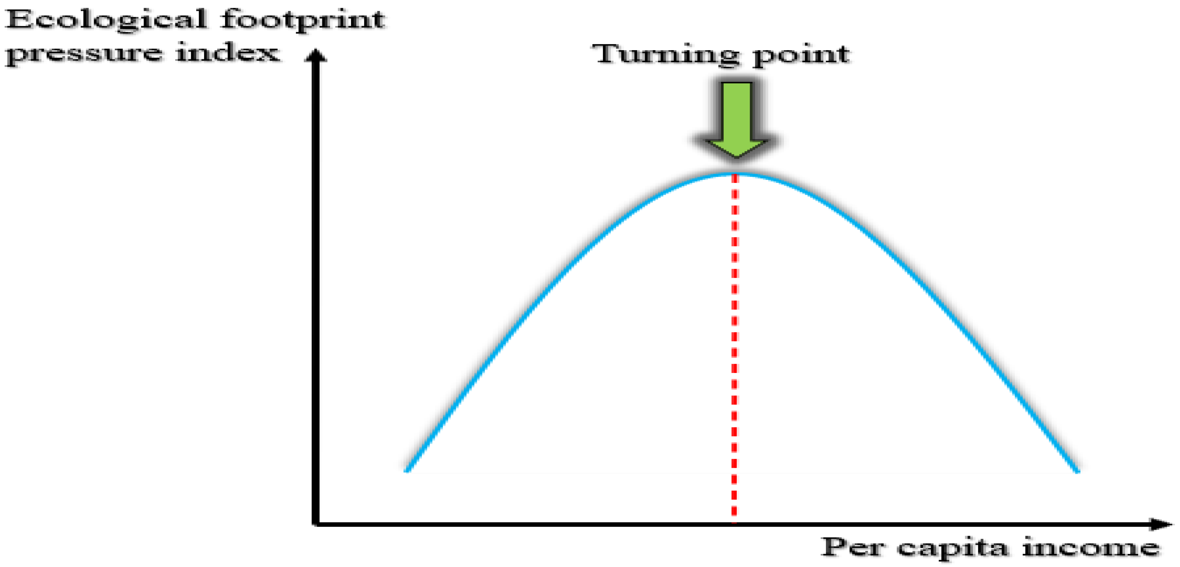Figure 1 illustrates the representation of the EKC hypothesis.

As seen in Figure 1, ecological pressure increases with an increase in per capita income during the initial stages of economic growth until reaching the turning point. This trend reverses after the turning point and ecological pressure decreases. In other words, the positive relationship between economic growth and ecological pressure at low-income levels is assumed to transform to a negative relationship between these parameters at high-income levels after the turning point. Within this context, the existence of the EKC hypothesis is confirmed if there is a hypothetical inverted U-shaped relationship between the EFPI and per capita income.

Based on the abovementioned background, the present study offers various contributions to and innovations for the current literature and differs from previous studies in the following aspects. First of all, to the best of our knowledge, the present study is the first to empirically analyze the effects of NRRs and REC, which are two crucial factors for sustainable growth and the environment, on the EFPI by using the same model within the context of the EKC hypothesis. In the majority of the previous studies, NRRs and REC have been analyzed separately in different models or their effects on CO₂ and EFP have been tested. Secondly, the number of studies investigating the relationship between NRRs and environmental degradation in the literature is insufficient. These studies present mixed results regarding the relationship between NRRs and environmental degradation; while some studies report that NRRs increase environmental degradation, others report a decrease. Therefore, further research is needed to examine the relationship between NRRs and environmental degradation. Thirdly, existing studies provide a limited perspective on environmental sustainability since they generally focus on either the demand side (EFP) or the supply side (biocapacity) of the environment. This study, by considering both the supply and demand dimensions of the environment via the EFPI, which represents environmental degradation, allows for a comprehensive analysis. In this regard, it significantly differs from the majority of previous studies. Furthermore, an innovative approach named MMQR, developed by Machado and Silva [43], is utilized in analyzing the empirical relationships between variables. This approach allows for more reliable results and accurate policy implications when compared to test methods that ignore the non-normal distribution and provide average predictions for variables.

The remaining sections of this study are organized as follows: Section 2 provides a summary of the literature review. Section 3 explains the data, and Section 4 introduces the methodology. Section 5 presents the empirical findings and discussion. The final section concludes this study and provides policy implications.

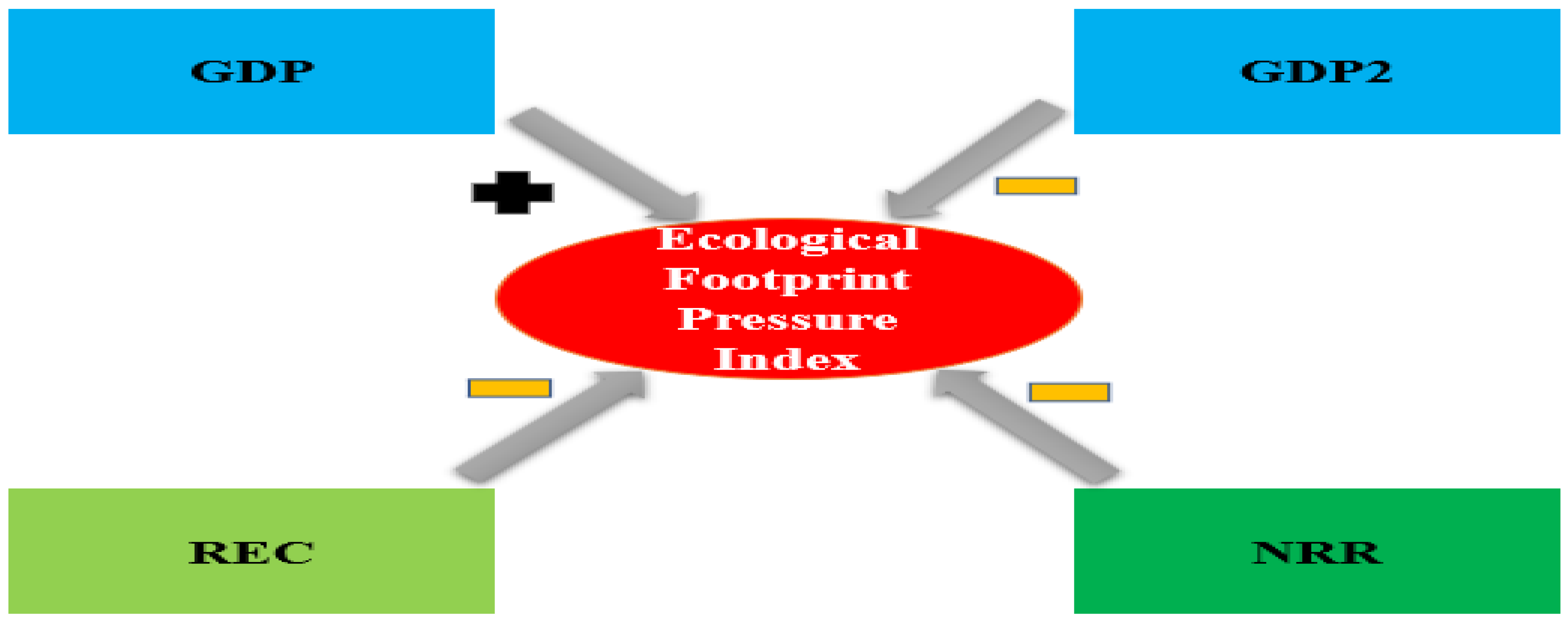
2. Literature Review

In the literature, there are many studies investigating the relationship between environmental degradation and REC and NRRs. These studies examine the correlations between the environment, renewable energy, and natural resources by using various environmental indicator variables and applying different estimation and causality methods for different time periods and countries or groups of countries. This section first presents the recent studies carried out on the nexus between renewable energy and environmental degradation. It then introduces the recent studies on the nexus between natural resource rents and environmental degradation.

2.1. The Studies on the Nexus between Renewable Energy and Environmental Degradation

There are many studies on the relationship between renewable energy and environmental degradation. Many of these studies have found that renewable energy decreases environmental degradation. Destek and Sinha [44], covering 24 OECD countries, found that renewable energy consumption reduced the ecological footprint for the period between 1980 and 2014. The findings also do not support the EKC hypothesis. Sharif et al. [45] examined the effect of renewable and non-renewable energy consumption on the ecological footprint in Türkiye for the period 1965Q1–2017Q4 by using the QARDL approach. The results confirmed the validity of the EKC hypothesis and revealed that renewable energy consumption has a decreasing effect on the ecological footprint. Fareed et al. [46] conducted an empirical analysis for Indonesia over the period 1965Q1–2014Q4 by utilizing the Fourier-based quantile causality test and concluded that renewable energy consumption enhances environmental quality. Sharma et al. [47] used data of eight developing countries in South and Southeast Asia from 1990 to 2015 to examine the role of renewable energy consumption on the ecological footprint by using the cross-sectional ARDL approach within the framework of the EKC hypothesis. The results supported the existence of an N-shaped EKC hypothesis and showed that renewable energy consumption contributes positively to environmental quality. Adebayo [48] used the novel wavelet coherence approach and found that renewable energy consumption improved the environmental quality in Spain over the period 1970Q1–2017Q4. The findings of Dogan and Pata [49] for G7 countries showed that renewable energy consumption positively affected the environmental quality over the years 1986–2017. The investigation of Fakher and Inglesi–Lotz [50] confirmed the validity of the EKC hypothesis for both OECD and OPEC countries and also revealed that renewable energy consumption enhances the environmental quality. Shang et al. [51] concluded that renewable energy consumption improved the environmental quality for ASEAN countries from 1980 to 2018. Adebayo and Samour [52] examined the relationship between fiscal policy, renewable energy, and the LCF in BRICS countries between 1990 and 2018 by making use of the novel panel Nonlinear Autoregressive Distributed Lag (P–NARDL) model. The empirical outcome indicates that renewable energy consumption plays an active role in improving the environmental quality. Employing the D–ARDL approach, Alola et al. [53] found that renewable energy consumption supported environmental sustainability by positively influencing the environmental quality in India during the period 1965–2018.

The prediction that renewable energy decreases environmental degradation has not been confirmed in all studies. There is also research that challenges the suggestion that renewable energy improves environmental quality and comes to the opposite conclusion. For example, Xu et al. [54] used the ARDL approach for the period 1970–2017 and concluded that renewable energy consumption had a negative effect on the environmental quality in Brazil. Caglar and Askin [55] examined the impact of renewable energy consumption on environmental quality in the top ten leading countries over the period 1990–2018. The CO₂ model did not yield any significant relationship; the LCF model showed that renewable energy consumption enhances environmental quality.

There is also research indicating no significant relationship between renewable energy and environmental degradation. Dong et al. [56] investigated the relationship between REC and CO₂ emissions in a panel of 120 countries from 1995 to 2015 within the context of the EKC hypothesis and found that REC does not significantly affect CO₂ emissions. Pata and Samour [42] investigated the effects of nuclear and renewable energy on CO₂ emissions in France from 1977 to 2017 by using Fourier co-integration and causality tests within the framework of the EKC hypothesis. The results supported the existence of the EKC hypothesis for the load capacity factor (LCF), but not for CO₂ emissions. Furthermore, renewable energy is found to have no statistically significant effect on the environment.

2.2. The Studies on the Nexus between Natural Resource Rents and Environmental Degradation

Total natural resources rents consist of the sum of oil rents, natural gas rents, coal rents (hard and soft), mineral rents, and forest rents. Interest in NRRs has grown with the rise in global warming and environmental degradation. Consequently, many researchers have explored the relationship between NRRs and environmental degradation. While contradictory findings can be found in the literature, a significant portion of these studies have identified a positive relationship between NRRs and environmental degradation.

Using the Pooled Mean Group ARDL method, Bekun et al. [57] found a positive relationship between NRRs and CO₂ emissions for selected EU-16 countries for the period 1996–2014. Ulucak et al. [18] used the AMG estimation method for OECD countries and concluded that NRRs positively affected CO₂ emissions during the period 1980–2016. The study of Huang et al. [58] used the QARDL method from 1995 to 2015 and provided evidence that NRRs increased CO₂ emissions in all quantiles in the United States. Using the CS-ARDL approach, Shen et al. [59] detected a positive relationship between NRRs and CO₂ emissions for 30 provinces of China in the period 1995–2017. Aladejare [60] concluded that NRRs increased the environmental degradation in the five richest African countries for the period between 1990 and 2019. Sarwat et al. [61] examined the existence of the EKC hypothesis in BRICS countries in the period 1990–2014 by making use of the MMQR approach. The results verified the validity of the EKC hypothesis and also indicated that NRRs increased CO₂ emissions across all quantiles. Adebayo et al. [62], covering 10 newly industrialized countries, used the MMQR approach to analyze the effect of NRRs on CO₂ emissions within the framework of the EKC from 1990 to 2018. The results confirmed the existence of the EKC hypothesis across all quantiles and revealed that NRRs positively affect CO₂ emissions and increase environmental degradation. Based on the data from 11 highly resource-consuming countries, Ni et al. [63] used the CS–ARDL method for the period between 1996 and 2019 and found that NRRs threaten environmental quality. Danish et al. [64] scrutinized the relationship between NRRs and CO₂ emissions in the US between 1985 and 2018 by using D–ARDL simulation and Kernel-based Regularized Least Squares techniques. The estimation results indicate that NRRs have a positive effect on CO₂ emissions.

Some of the studies in the literature report that the effect of NRRs on environmental degradation is negative. Alfalih and Hadj [65] investigated the dynamic effects of natural resource rents on environmental sustainability in Saudi Arabia for 1985–2017 under low- and high-sustainability regimes. The results point to the role of NRRs in enhancing environmental sustainability. For the case of Sudan, Alnour et al. [66] used the Structural Vector Autoregressive (SVAR) model for the period 1990Q1–2018Q1 and concluded that NRRs have a negative effect on environmental degradation. Arslan et al. [67] examined the dynamics of NRRs, environmental sustainability, and sustainable economic growth in China for the period of 1970 to 2016 by using the Generalized Method of Moments, Dynamic Ordinary Least Squares, and Robust Least Squares estimations. They found that NRRs contribute to environmental sustainability by reducing CO₂ emissions and ecological footprint at the expense of economic growth. Using the CS-ARDL test, Chen et al. [68] focused on the top ten polluted nations for the period between 1990 and 2019. The results showed that NRRs have a positive effect on eco-efficiency. Zheng et al. [69] examined the effect of NRRs, renewable energy, and economic growth on three different environmental quality indicators (CO₂ emissions, EFP, LCF) in China over the period of 1990Q1–2018Q4 by using Bootstrap Fourier Granger causality in quantiles. The results demonstrated that NRRs support environmental quality.

There are also studies in the literature, albeit few, with mixed results. For example, Alvarado et al. [70] explored the role of NRRs and economic complexity on the ecological footprint in Latin American countries by making use of the quantile regression approach. The results demonstrated that the effect of NRRs on the ecological footprint is mixed. Zuo et al. [20] utilized the AMG test for 90 Belt and Road Initiative countries over the period 1991–2018. The estimation results showed that NRRs alone lead to environmental degradation, whereas they, in conjunction with technological innovation (NRRs x TI), help to increase environmental quality. Jahanger et al. [71] analyzed the relationships between NRRs, energy use, human capital, and greenhouse gas (GHG) emissions in the BRICS countries during the period 1990–2018 by making use of the panel quantile regression method. The results revealed a positive relationship between NRRs and GHG emissions in lower quantiles, while a negative relationship was observed between NRRs and GHG emissions in higher quantiles.

In this context, there are many studies in the literature that have empirically analyzed the EKC hypothesis from various perspectives for different countries and regions. However, to the best of our knowledge, there is no study in the literature that evaluates the effect of both NRRs and REC on the EFPI, which considers the supply and demand dimensions of the environment, in the context of the EKC hypothesis specifically for the ASEAN-5 countries.

3. Data

This study investigates the effects of renewable energy consumption and natural resource rents on environmental degradation within the context of the EKC hypothesis. The data used in the present study were obtained from two different sources. The ecological footprint and biocapacity data, of which the EFPI is composed, were obtained from the Global Footprint Network [10]. The EFPI is calculated by dividing the per capita ecological footprint by the per capita biocapacity. Economic growth (GDP), renewable energy consumption (REC), and natural resource rent (NRR) data were collected from the World Development Indicators Database [22]. The EFPI, which is used as the indicator of environmental degradation in this study, is the dependent variable. GDP, GDP², REC, and NRRs are the explanatory variables.

The ecological footprint and biocapacity are two important concepts that lay the foundation of ecological calculations regarding sustainable development. While the ecological footprint measures human activities’ demand for natural resources, biocapacity represents the amount of resources that nature provides to meet this demand. The traditional ecological footprint model evaluates the pressure that humans exert on nature, how quickly they consume natural resources, and the environmental impacts of this consumption, offering a one-dimensional perspective. This ecological footprint model focuses on the demand side of the environment, often neglecting biocapacity, which typically represents the supply side of nature. However, disregarding biocapacity can lead to an incomplete or incorrect valuation of the production’s ability to meet consumption. Moreover, compensating or balancing environmental damage with the existing biocapacity enables the promotion of sustainable development. Therefore, the ecological footprint should be addressed simultaneously with biocapacity. This way, more accurate assessments and policy implications regarding environmental sustainability can be made. In this sense, the EFPI simultaneously considers the supply and demand dimensions, providing a broader perspective on environmental sustainability and risks and allowing for a more accurate assessment of consumption’s environmental impact. Therefore, when determining Sustainable Development Goals and evaluating ecological footprints, using the EFPI provides a stronger and more comprehensive understanding. Wang et al. [40] developed the EFPI by simultaneously considering ecological footprint and biocapacity. The EFPI is calculated by using the formula in Equation (1):

$$\mathrm{E}\mathrm{F}\mathrm{P}\mathrm{I}=\frac{\mathrm{E}\mathrm{c}\mathrm{o}\mathrm{l}\mathrm{o}\mathrm{g}\mathrm{i}\mathrm{c}\mathrm{a}\mathrm{l} \mathrm{F}\mathrm{o}\mathrm{o}\mathrm{t}\mathrm{p}\mathrm{r}\mathrm{i}\mathrm{n}\mathrm{t}}{\mathrm{B}\mathrm{i}\mathrm{o}\mathrm{a}\mathrm{p}\mathrm{a}\mathrm{c}\mathrm{i}\mathrm{t}\mathrm{y}}$$

(1)

Considering Equation (1), the relationship between ecological footprint and biocapacity is explained within the framework of the sustainable environment as follows:

When 0 < EFPI < 1, ecological resource supply (biocapacity) exceeds ecological resource demand (ecological footprint).

EFPI = 1: Ecological footprint is equal to biocapacity. In other words, ecological resource supply is equal to ecological resource demand.

EFPI > 1: Ecological footprint exceeds biocapacity. That is to say, ecological resource demand is higher than ecological resource supply.

To achieve a sustainable environment, the EFPI should be between “0” and “1” (0 < EFPI < 1). This situation indicates that environmental conditions are safe and sustainable. In cases where environmental conditions are safe and sustainable, the sustainable use of natural resources can be successfully achieved. The case of EFPI = 1 refers to ecological balance and a critical level of sustainability. In other words, environmental conditions are now at a critical ecological insecurity threshold. The case of EFPI > 1 indicates that the environment is under threat. In this scenario, resource supply reaches a level that cannot meet human consumption demands, leading to concerns about environmental sustainability.

Table 1. Variables, measurements, and data sources.

Variable	Symbol	Measurement	Signs	Source
Ecological footprint pressure index	EFPI	Global hectares	N/A	GFN
Economic growth	GDP	GDP per capita (constant 2015 USD)	+	WB
Square of economic growth	GDP2	Square of GDP per capita	–	WB
Renewable energy consumption	REC	% of total final energy consumption	–	WB
Natural resource rents	NRR	Total natural resources rents (% of GDP)	+/−	WB

shows variables, measurements, and data sources.

Established in the study carried out by Zheng et al. [69], the empirical model is presented in Equation (2):

$${\mathrm{l}\mathrm{n}\mathrm{E}\mathrm{F}\mathrm{P}\mathrm{I}}_{\mathrm{i}\mathrm{t}}={{\mathsf{\beta }}_0+{\mathsf{\beta }}_1\mathrm{l}\mathrm{n}\mathrm{G}\mathrm{D}\mathrm{P}}_{\mathrm{i}\mathrm{t}}+{{\mathsf{\beta }}_2\mathrm{l}\mathrm{n}\mathrm{G}\mathrm{D}\mathrm{P}}_{\mathrm{i}\mathrm{t}}^2{+{\mathsf{\beta }}_3\mathrm{l}\mathrm{n}\mathrm{R}\mathrm{E}\mathrm{C}}_{\mathrm{i}\mathrm{t}}{+{{\mathsf{\beta }}_4\mathrm{l}\mathrm{n}\mathrm{N}\mathrm{R}\mathrm{R}}_{\mathrm{i}\mathrm{t}}+\mathsf{\epsilon }}_{\mathrm{i}\mathrm{t}}$$

(2)

where i illustrates cross-sections and t represents the period (1990–2018). lnEFPI, lnGDP, lnGDP², lnREC, and lnNRR denote the logarithm data of all variables. Economic growth causes environmental damage by stimulating the pressure on the environment. Therefore, GDP is expected to positively affect the EFPI $\left({\mathsf{\beta }}_1=\frac{\partial \mathrm{G}\mathrm{D}\mathrm{P}}{\partial \mathrm{E}\mathrm{F}\mathrm{P}\mathrm{I}}>0\right)$. On the other hand, GDP² is expected to affect the EFPI negatively $\left({\mathsf{\beta }}_2=\frac{\partial \mathrm{G}{\mathrm{D}\mathrm{P}}^2}{\partial \mathrm{E}\mathrm{F}\mathrm{P}\mathrm{I}}<0\right)$. Clean energy consumption is an important factor for environmental sustainability. As a clean and alternative source, renewable energy helps to preserve the environment. Within this context, REC is expected to be negative $\left({\mathsf{\beta }}_3=\frac{\partial \mathrm{R}\mathrm{E}\mathrm{C}}{\partial \mathrm{E}\mathrm{F}\mathrm{P}\mathrm{I}}<0\right)$. NRRs have a mixed effect on environmental degradation. Natural resources are excessively used as a result of the rapid economic growth efforts around the world. In this process, economic growth causes an excessive use of resources by exceeding the source replenishment capacity [15]. Therefore, increases in NRRs might have an effect on increasing the EFPI. Thus, the NRR coefficient (${\mathsf{\beta }}_4$) is expected to be positive $\left({\mathsf{\beta }}_4=\frac{\partial \mathrm{N}\mathrm{R}\mathrm{R}}{\partial \mathrm{E}\mathrm{F}\mathrm{P}\mathrm{I}}>0\right)$. On the other hand, redirecting natural resource revenues towards environmentally friendly production and consumption processes that support sustainable production and management practices can improve the environmental quality. Thus, it is possible to prevent the uncontrolled use of natural resources and make more efficient use of them. Within this context, the NRR coefficient (${\mathsf{\beta }}_4$) is expected to be negative $\left({\mathsf{\beta }}_4=\frac{\partial \mathrm{N}\mathrm{R}\mathrm{R}}{\partial \mathrm{E}\mathrm{F}\mathrm{P}\mathrm{I}}<0\right)$.

4. Methodology

A flowchart of the empirical methodology is shown in Figure 2. A six-step methodology is followed to investigate the effects of REC and NRRs on environmental degradation in the context of the EKC hypothesis.

• In the first step, the presence of cross-sectional dependence (CSD) is determined by using the Breusch–Pagan [72] Lagrange Multiplier (LM) test, Pesaran’s [73] scaled LM test, Baltagi et al.’s [74] bias-corrected scaled LM test, and Pesaran’s [73] CD test. Then, the existence of slope heterogeneity is analyzed using the Delta ($\widetilde{∆}$ test) and Adjusted Delta (${\widetilde{∆}}_{\mathrm{a}\mathrm{d}\mathrm{j}.}$) tests developed by Pesaran and Yamagata [75].
• In the second step, the stationary properties of the variables are examined by utilizing Pesaran’s [76] cross-sectionally IPS (CIPS) and cross-sectionally ADF (CADF) panel unit root tests.
• In the third step, a co-integration relationship between the variables is researched by employing the panel LM co-integration test introduced by Westerlund and Edgerton [77].
• In the fourth step, the normal distribution of the variables is checked using the normality tests proposed by Chen and Shapiro [78] and Shapiro and Wilk [79].
• In the fifth step, the novel MMQR approach presented by Machado and Silva [43], FE–OLS, FMOLS, and DOLS tests are used for coefficient estimation.
• In the sixth step, the Granger non-causality test developed by Dumitrescu and Hurlin [80] is conducted to determine the direction of the relationship between the variables.

4.1. Cross-Sectional Dependence

In the first step, the presence of the CSD is tested using Breusch–Pagan [72] LM, Pesaran’s [73] scaled LM, Baltagi et al.’s [74] bias-corrected scaled LM, and Pesaran’s [73] CD tests.

When N is fixed and T → ∞, Breusch–Pagan [72] LM is a reliable CSD test. The LM test statistic is expressed in Equation (3):

$$\mathrm{L}\mathrm{M}=\mathrm{T}\sum _{\mathrm{i}=1}^{\mathrm{N}-1}\sum _{\mathrm{j}=\mathrm{i}+1}^{\mathrm{N}}{\widehat{\mathrm{p}}}_{\mathrm{i}\mathrm{j}}^2$$

(3)

For infinite T and N panels (T → ∞ and N → ∞), Pesaran [73] suggests a scaled LM test. The test statistic is defined in Equation (4):

$${\mathrm{C}\mathrm{D}}_{\mathrm{s}\mathrm{c}\mathrm{a}\mathrm{l}\mathrm{e}\mathrm{d} \mathrm{L}\mathrm{M}}={\left(\frac{1}{\mathrm{N}(\mathrm{N}-1)}\right)}^{1/2}\sum _{\mathrm{i}=1}^{\mathrm{N}-1}\sum _{\mathrm{j}=\mathrm{i}+1}^{\mathrm{N}}\left(\mathrm{T}{\widehat{\mathrm{p}}}_{\mathrm{i}\mathrm{j}}^2-1\right)$$

(4)

In panels with N > T, the lack of a CSD test that can yield robust results is met by using the CD test of Pesaran [73]. The CD test statistic is given in Equation (5):

$$\mathrm{C}\mathrm{D}=\sqrt{\left(\frac{2\mathrm{T}}{\mathrm{N}(\mathrm{N}-1)}\right)}\sum _{\mathrm{i}=1}^{\mathrm{N}-1}\sum _{\mathrm{j}=\mathrm{i}+1}^{\mathrm{N}}{\widehat{\mathrm{p}}}_{\mathrm{i}\mathrm{j}}$$

(5)

Baltagi et al. [74] developed the bias-corrected scaled LM test that is relatively newer and more robust. The test statistic is shown in Equation (6):

$${\mathrm{L}\mathrm{M}}_{\mathrm{B}\mathrm{C} \mathrm{s}\mathrm{c}\mathrm{a}\mathrm{l}\mathrm{e}\mathrm{d}}=\sqrt{\left(\frac{1}{\mathrm{N}(\mathrm{N}-1)}\right)}\sum _{\mathrm{i}=1}^{\mathrm{N}-1}\sum _{\mathrm{j}=\mathrm{i}+1}^{\mathrm{N}}\left({\mathrm{T}}_{\mathrm{i}\mathrm{j}}^{{\widehat{\mathrm{p}}}^2}-1\right)-\frac{\mathrm{N}}{2\left(\mathrm{T}-1\right)}\to \mathrm{N}\left(\mathrm{0,1}\right)$$

(6)

4.2. Panel Unit Root Test

Traditional unit root tests assume cross-sectional independence and slope homogeneity when examining the stationarity properties of variables. Therefore, the first-generation unit root tests are not reliable in the presence of CSD and slope heterogeneity. Considering such disadvantages, Pesaran [76] suggests the cross-sectionally augmented Dickey–Fuller (CADF) test, which regards CSD and slope heterogeneity. Moreover, the average of unit root statistics for cross-sections is calculated to obtain the cross-sectionally IPS (CIPS) test statistic. The CIPS test statistic is given in Equation (7):

$$\mathrm{C}\mathrm{I}\mathrm{P}\mathrm{S}={\mathrm{N}}^{-1}\sum _{\mathrm{i}=1}^{\mathrm{n}}{\mathrm{C}\mathrm{A}\mathrm{D}\mathrm{F}}_{\mathrm{i}}$$

(7)

In Equation (7), CADF_i refers to the CADF t-test statistic for each section in CADF regression.

4.3. Panel Co-Integration Tests

Classical co-integration tests examine the long-term relationships between variables by ignoring the CSD and slope heterogeneity. To address this limitation, Westerlund and Edgerton [77] developed the panel LM co-integration test that allows for CSD and slope heterogeneity. The LM co-integration test is reliable even in small-sample properties of the panel. The LM test statistic is presented in Equation (8):

$${\mathrm{L}\mathrm{M}}_{\mathrm{N}}^{+}=\frac{1}{\mathrm{N}{\mathrm{T}}^2}\sum _{\mathrm{i}=1}^{\mathrm{N}}\sum _{\mathrm{t}=\mathrm{i}}^{\mathrm{T}}{\widehat{\mathsf{\omega }}}_{\mathrm{i}}^{-2}{\mathrm{S}}_{\mathrm{i}\mathrm{t}}^2$$

(8)

${\mathrm{S}}_{\mathrm{i}\mathrm{t}}$ refers to the partial total process of the error term, whereas ${\widehat{\mathsf{\omega }}}_{\mathrm{i}}^2$ denotes the long-term variance of the error term.

4.4. Panel Method of Moments Quantile Regression Approach

Ordinary Least Squares regression models provide partial information in coefficient estimation since they consider average effects. On the other hand, quantile-based estimation methods estimate the effects of explanatory variables on different points or locations of the dependent variable more comprehensively. Therefore, it is stated that quantile-based regression estimates are stronger compared to basic regression estimates. In this study, the novel MMQR approach developed by Machado and Silva [43] is utilized as the main estimation method for long-term coefficient estimation. The reason for preferring the MMQR approach is its higher reliability when compared to other methods such as ordinary panel quantile regression tests, DOLS, and FMOLS. From this aspect, the advantages of the MMQR approach are as follows: (i) The MMQR approach is a favorable method for controlling individual effects and endogeneity. (ii) It is useful for examining the effects of heterogeneity at various quantiles. (iii) It yields reliable results on the existence of asymmetry, nonlinearity, and non-normal distribution in variables. (iv) It is sensitive to outliers.

The MMQR equation of this study is rendered as follows:

$${\mathrm{Q}}_{\mathrm{Y}}\left(\mathsf{\tau }/{\mathrm{X}}_{\mathrm{i}\mathrm{t}}\right)=\left({\mathsf{\alpha }}_{\mathrm{i}}+{\mathsf{\delta }}_{\mathrm{i}}\mathrm{q}\left(\mathsf{\tau }\right)\right)+{\mathrm{X}}_{\mathrm{i}\mathrm{t}}^{\prime }\mathsf{\beta }+{\mathrm{Z}}_{\mathrm{i}\mathrm{t}}^{\prime }\mathsf{\gamma }\mathrm{q}\left(\mathsf{\tau }\right)$$

(9)

In Equation (9), ${\mathrm{X}}_{\mathrm{i}\mathrm{t}}$ is the vector of GDP, GDP², REC, and NRRs, which are explanatory variables, whereas ${\mathrm{Q}}_{\mathrm{Y}}\left(\mathsf{\tau }/{\mathrm{X}}_{\mathrm{i}\mathrm{t}}\right)$ represents the quantile distribution (Y_it) of the dependent variable of the EFPI.

4.5. Panel Causality Approach

Granger [81] introduced the time-series-based Granger causality test in order to determine the direction of causality between variables. Holtz–Eakin et al. [82] adapted the time-series-based Granger causality test to the panel data analysis and developed the panel VAR-based Granger non-causality test. On the other hand, traditional panel causality tests have limited power due to their assumption of slope homogeneity and cross-sectional independence. Therefore, in this study, the Granger non-causality test introduced by Dumitrescu and Hurlin [80] is used instead of traditional Granger causality tests. The strengths of this test are explained as follows: (i) This test allows for CSD and slope heterogeneity. (ii) It is reliable even in unbalanced panels. (iii) It can also be applied to panels where the cross-sectional dimension (N) is larger than the time dimension (T). (iv) It yields robust results, even in relatively small-sample panels.

In order to test the panel causality, Dumitrescu and Hurlin [80] introduced the following linear model:

$${\mathrm{y}}_{\mathrm{i},\mathrm{t}}={\mathsf{\alpha }}_{\mathrm{i}}+{\sum }_{\mathrm{k}=1}^{\mathrm{K}}{\mathsf{\gamma }}_{\mathrm{i}}^{\left(\mathrm{k}\right)}{\mathrm{y}}_{\mathrm{i}, \mathrm{t}-\mathrm{k}}+{\sum }_{\mathrm{k}=1}^{\mathrm{K}}{\mathsf{\beta }}_{\mathrm{i}}^{\left(\mathrm{k}\right)}{\mathrm{x}}_{\mathrm{i}, \mathrm{t}-\mathrm{k}}+{\mathsf{\epsilon }}_{\mathrm{i},\mathrm{t}}$$

(10)

where ${\mathsf{\alpha }}_{\mathrm{i}}$ = the individual fixed effects, ${\mathsf{\gamma }}_{\mathrm{i}}^{\left(\mathrm{k}\right)}$ = the autoregressive parameters, K = the lag orders, and ${\mathsf{\beta }}_{\mathrm{i}}^{\left(\mathrm{k}\right)}$ = the regression slope parameters. ${\mathrm{y}}_{\mathrm{i}, \mathrm{t}}$ and ${\mathrm{x}}_{\mathrm{i}, \mathrm{t}}$ show the stationary variables in period t for each i.

The hypotheses supposed for the Dumitrescu and Hurlin [80] Granger non-causality test are shown as follows:

$$\begin{gathered} {\mathrm{H}}_0:{\mathsf{\beta }}_{\mathrm{i}}=0\forall \mathrm{i}=1,\dots ,\mathrm{N} \\ {\mathrm{H}}_{\mathrm{A}}:{\mathsf{\beta }}_{\mathrm{i}}=0\forall \mathrm{i}=1,\dots ,{\mathrm{N}}_1 \\ {\mathsf{\beta }}_{\mathrm{i}}\ne 0\forall \mathrm{i}={\mathrm{N}}_1+1,{\mathrm{N}}_1+2,\dots ,\mathrm{N} \end{gathered}$$

The null hypothesis assumes no causality in a homogeneous panel, whereas the alternative hypothesis assumes causality in at least one cross-section in a heterogeneous panel. If the probability values are smaller than the significance values, the null hypothesis is rejected. Otherwise, when the probability values are higher than the significance values, the null hypothesis cannot be rejected.

Dumitrescu and Hurlin [80] separately calculate individual Wald test statistics for each cross-sectional unit. The panel Wald statistic is obtained by taking the average of individual Wald test statistics. The panel Wald statistic is given in Equation (11):

$${\mathrm{W}}_{\mathrm{N},\mathrm{T}}^{\mathrm{H}\mathrm{n}\mathrm{c}}=\frac{1}{\mathrm{N}}{\sum }_{\mathrm{i}=1}^{\mathrm{N}}{\mathrm{w}}_{\mathrm{i},\mathrm{T}}$$

(11)

In Equation (11), ${\mathrm{w}}_{\mathrm{i},\mathrm{T}}$ denotes the individual Wald test statistics.

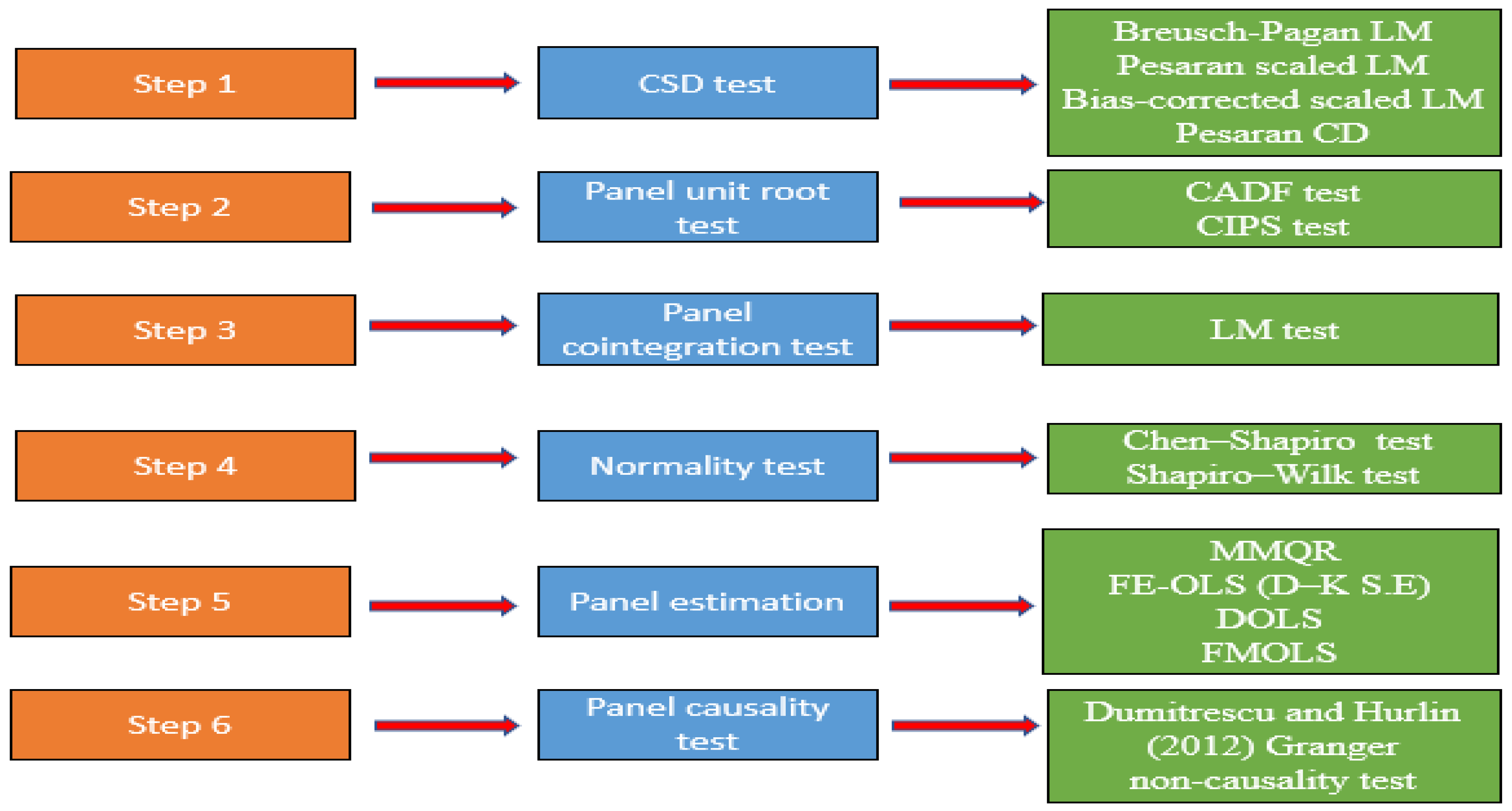
5. Empirical Findings and Discussion

The presence of CSD is determined using Breusch–Pagan LM, Pesaran scaled LM, bias-corrected scaled LM, and Pesaran CD tests. The CSD test results are given in

Table 2. CSD test results.

Variables	Breusch–Pagan LM	Pesaran Scaled LM	Bias-Corrected Scaled LM	Pesaran CD
EFPI	92.336 a	18.410 a	18.310 a	5.326 a
GDP	242.833 a	52.063 a	51.963 a	15.579 a
GDP2	243.285 a	52.164 a	52.064 a	15.594 a
REC	98.573 a	19.805 a	19.705 a	3.784 a
NRR	45.691 a	7.980 a	7.880 a	1.748 c

Note: ^a and ^c indicate significance at 1% and 10% levels, respectively.

.

Given all the CSD test results in Table 2, the null hypothesis assuming no CSD is rejected for all variables, which indicates the presence of CSD in all variables. This result demonstrates that a shock observed in any of the ASEAN-5 countries influences other countries in the panel as well. Subsequently, slope heterogeneity is examined using the Delta ($\widetilde{∆}$ test) and Adjusted Delta (${\widetilde{∆}}_{\mathrm{a}\mathrm{d}\mathrm{j}.}$) tests. The results of the slope heterogeneity test are shown in

Table 3. Slope heterogeneity test results.

lnEFPI = f (lnGDP, lnGDP2, lnREC, lnNRR)	Test Statistic	p-Value
$\widetilde{∆}$ test	9.381 a	0.000
${\widetilde{∆}}_{\mathrm{a}\mathrm{d}\mathrm{j}.}$ test	10.534 a	0.000

Note: ^a represents significance at the 1% level.

.

Given the $\widetilde{∆}$ and ${\widetilde{∆}}_{\mathrm{a}\mathrm{d}\mathrm{j}.}$ test results in Table 3, the null hypothesis assuming the presence of slope homogeneity is rejected at the significance level of 1% and it is determined that there is slope heterogeneity. It suggests that slope coefficients differ between cross-sections. After determining the presence of CSD and slope heterogeneity, the stationarity characteristics of variables are examined utilizing CADF and CIPS tests. The panel unit root test results are presented in

Table 4. Panel unit root test results.

	CADF Test		CIPS Test
Variables	Level	First Difference	Level	First Difference
EFPI	–0.982	–3.491 a	–0.975	–3.491 a
GDP	–2.083	–3.270 a	–1.937	–3.231 a
GDP2	–2.020	–3.358 a	–1.891	–3.270 a
REC	–1.401	–3.010 a	–1.133	–2.903 a
NRR	–1.429	–3.942 a	–1.429	–4.029 a

Note: ^a indicates significance at the 1% level.

.

Based on the results of the CADF and CIPS tests presented in Table 4, the null hypothesis supposing the presence of a unit root cannot be rejected for any variables at the 1% level, and it is determined that all variables have a unit root at the level. On the other hand, when first differences are calculated, it is observed that the null hypothesis is rejected at the significance level of 1% for all variables. The findings indicate that all variables are stationary at the first difference. After determining the unit root characteristics of the variables, long-term relationships between the variables are investigated using the panel LM co-integration test. The results of the panel co-integration test are shown in

Table 5. Panel co-integration test results.

LM Test	Test Statistic	Asymptotic p-Value	Bootstrap p-Value
Constant	0.860	1.000	0.195
Constant and trend	4.471	0.000	0.998

.

In the panel LM co-integration test results shown in Table 5, the asymptotic p-value is valid when there is no CSD, whereas the bootstrap p-value is valid when CSD is present. Since it is found that CSD exists in the present study, the decision regarding whether the variables are co-integrated or not is made by examining the bootstrap p-value. Given the bootstrap p-value, the null hypothesis assuming the existence of a co-integration relationship cannot be rejected in both constant and constant and trend models. Therefore, it is concluded that the variables move together in the long run; in other words, they are co-integrated. After determining that the variables are co-integrated, normality tests as proposed by Chen and Shapiro [78] and Shapiro and Wilk [79] are conducted to check if the variables follow a normal distribution. The results of the normality tests are presented in

Table 6. Normality test results.

Variables	Chen–Shapiro Test		Shapiro–Wilk Test
	Test Statistic	p-Value	Test Statistic	p-Value
EFPI	0.805 a	0.000	0.639 a	0.000
GDP	0.938 a	0.000	0.869 a	0.000
GDP2	0.924 a	0.000	0.843 a	0.000
REC	0.910 a	0.000	0.817 a	0.000
NRR	0.866 a	0.000	0.740 a	0.000

Note: ^a indicates significance at the 1% level.

.

Given the normality test results in Table 6, the null hypothesis supposing a normal distribution of the variables is rejected at the significance level of 1% for all variables. Thus, it is concluded that the variables EFPI, GDP, GDP², REC, and NRRs are not normally distributed. The normality test results demonstrate that the quantile regression approach is more reliable and appropriate for long-term coefficient estimation. Therefore, MMQR is adopted in the present study. The MMQR results are provided in

Table 7. Results of methods of moments quantile regression (MMQR).

Variables	Quantiles
	0.1	0.2	0.3	0.4	0.5	0.6	0.7	0.8	0.9
GDP	2.349 a	2.562 a	2.829 a	3.016 a	3.192 a	3.399 a	3.595 a	3.802 a	4.152 a
GDP2	–0.124 a	–0.136 a	–0.152 a	–0.163 a	–0.173 a	–0.185 a	–0.197 a	–0.209 a	–0.229 a
REC	–0.166 c	–0.175 b	–0.185 a	–0.193 a	–0.200 a	–0.208 a	–0.216 a	–0.224 a	–0.238 b
NRRs	–0.061 c	–0.062 b	–0.064 a	–0.065 a	–0.066 a	–0.067 a	–0.069 a	–0.070 b	–0.072 c

Note: ^a–c indicate significance at 1%, 5%, and 10% levels, respectively.

.

The MMQR results in Table 7 reveal that GDP has a positive and significant effect on the EFPI in all quantiles, whereas GDP² has a negative and significant effect on the EFPI in all quantiles. Based on this finding, the validity of the EKC hypothesis, which assumes an inverted U-shaped relationship between the EFPI and GDP, is verified. Accordingly, increases in GDP in ASEAN-5 countries initially increase environmental degradation until the turning point, after which they have a reducing effect on environmental degradation. In this sense, a 1% increase in GDP leads to increases by 2.349% (0.1), 2.562% (0.2), 2.829% (0.3), 3.016% (0.4), 3.192% (0.5), 3.399% (0.6), 3.595% (0.7), 3.802% (0.8), and 4.152% (0.9) in the EFPI. Conversely, a 1% increase in GDP² results in decreases of −0.124% (0.1), −0.136% (0.2), −0.152% (0.3), −0.163% (0.4), −0.173% (0.5), −0.185% (0.6), −0.197% (0.7), −0.209% (0.8), and −0.229% (0.9) in the EFPI.

REC is found to have a negative and statistically significant effect on the EFPI. This finding proves that the use of clean and sustainable resources such as renewable energy is an important factor in order to reduce environmental pressure. Accordingly, a 1% increase in REC reduces the EFPI by −0.166% (0.1), −0.175% (0.2), −0.185% (0.3), −0.193% (0.4), −0.200% (0.5), −0.208% (0.6), −0.216% (0.7), −0.224% (0.8), and −0.238% (0.9). These findings are consistent with the results of Adebayo [48], Adebayo and Samour [52], Alola et al. [53], Destek and Sinha [44], Dogan and Pata [49], Fakher and Inglesi–Lotz [50], Shang et al. [51], and Sharif et al. [45]. However, these findings contradict the results of the study carried out by Xu et al. [54].

NRRs are found to have a negative and statistically significant effect on the EFPI. This finding demonstrates that income derived from natural resources in ASEAN-5 countries has a reducing effect on environmental degradation. In other words, NRRs support a sustainable environment. Therefore, a 1% increase in NRRs reduces the EFPI by –0.061% (0.1), −0.062% (0.2), −0.064% (0.3), −0.065% (0.4), −0.066% (0.5), −0.067% (0.6), −0.069% (0.7), −0.070% (0.8), and −0.072% (0.9). These findings are similar to those of Arslan et al. [67], Chen et al. [68], Jahanger et al. [71] (for higher quantiles), Zheng et al. [69], and Zuo et al. [20]. However, they also contradict the results reported by Adebayo et al. [62], Aladejare [60], Alnour et al. [66], Bekun et al. [57], Danish et al. [64], Huang et al. [58], Ni et al. [63], Sarwat et al. [61], Shen et al. [59], and Ulucak et al. [18].

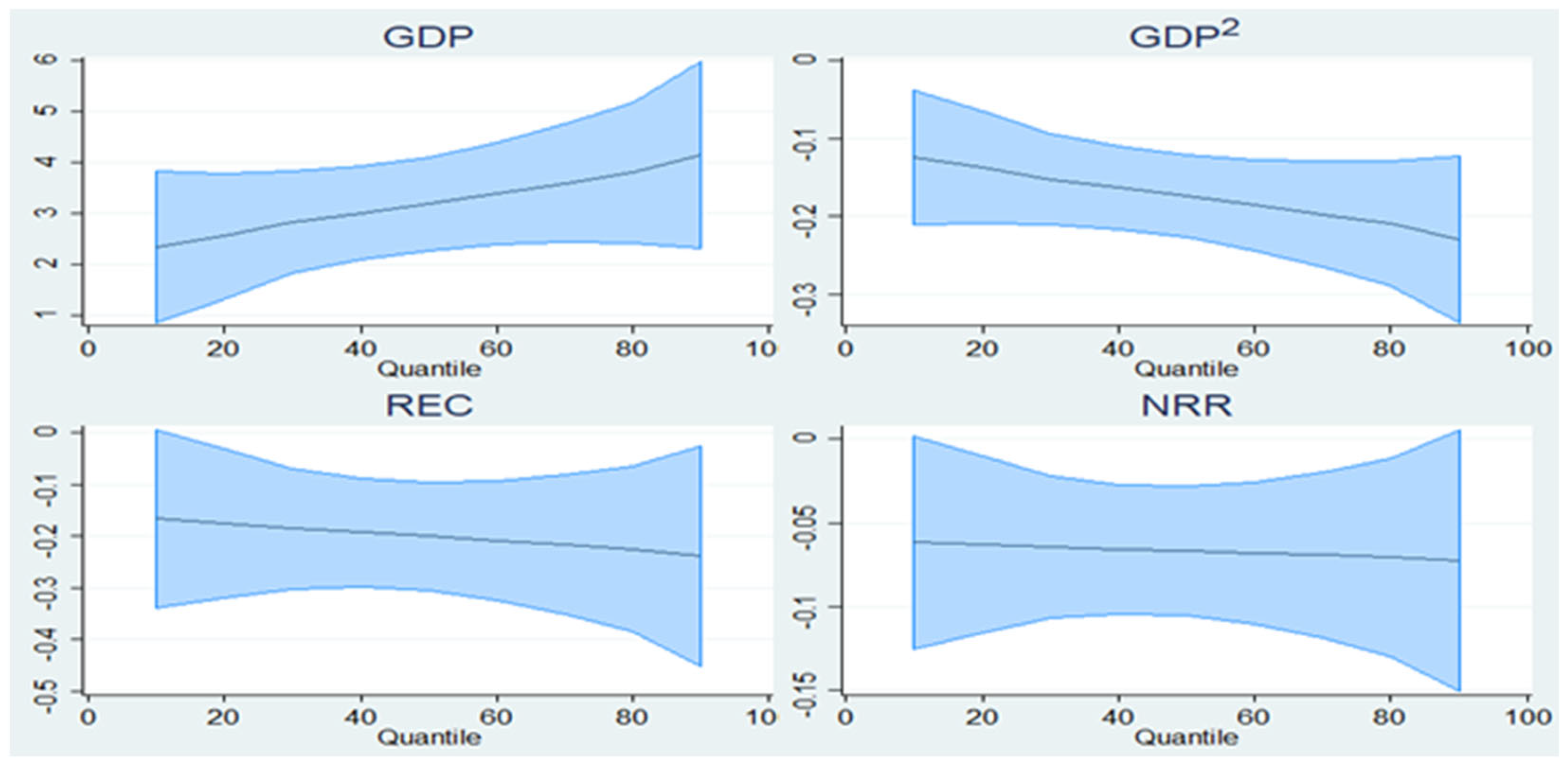
Figure 3 shows graphical plots of MMQR. Accordingly, Figure 3 demonstrates the relationship between dependent variables of the EFPI and explanatory variables (GDP, GDP², REC, NRRs) in different quantiles. For a robustness check and comparison, in addition to the MMQR approach, FE–OLS, DOLS, and FMOLS estimations are employed in the present study. Results of the panel estimation are shown in

Table 8. Results of panel estimation.

Variables	FE–OLS (D–K S.E)			DOLS			FMOLS
	Coeff.	t-Stats	p-Value	Coeff.	t-Stats	p-Value	Coeff.	t-Stats	p-Value
GDP	3.168 a	7.76	0.000	5.583 a	6.899	0.000	3.329 a	6.054	0.000
GDP2	–0.172 a	–6.51	0.000	–0.312 a	–7.294	0.000	–0.186 a	–6.147	0.000
REC	–0.199 a	–4.03	0.000	–0.122 b	–2.520	0.013	–0.225 a	–3.688	0.000
NRR	–0.066 a	–2.76	0.010	–0.068 b	–2.440	0.016	–0.065 b	–2.011	0.046

Note: ^a and ^b indicate significance at 1% and 5% levels, respectively. D–K S.E: Driscoll–Kraay standard errors.

.

According to the estimation results from the FE–OLS, DOLS, and FMOLS panel in Table 8, the coefficients of GDP and GDP² are statistically significant and have positive and negative signs, respectively. This result implies an inverted U-shaped relationship between the EFPI and GDP, confirming the EKC hypothesis. Therefore, a 1% increase in GDP leads to a respective increase of 3.168%, 5.583%, and 3.329% in the EFPI according to FE–OLS, DOLS, and FMOLS. Conversely, a 1% increase in GDP² causes a decrease of −0.172%, −0.312%, and −0.186% in the EFPI for FE–OLS, DOLS, and FMOLS, respectively. These findings support the results of MMQR. On the other hand, the coefficients of REC and NRRs are statistically significant and negative. In other words, an increase in REC and NRRs reduces the EFPI. Therefore, a 1% increase in REC leads to a respective decrease of −0.199%, −0.122%, and −0.225% in the EFPI for FE–OLS, DOLS, and FMOLS. Similarly, a 1% increase in NRRs causes a respective decrease of −0.066%, −0.068%, and −0.065% in the EFPI for FE–OLS, DOLS, and FMOLS. These findings are consistent with the results of MMQR. Therefore, the findings of FE–OLS, DOLS, and FMOLS affirm the reliability and robustness of the MMQR estimates. Figure 4 represents a summary of the long-term estimation results.

The results of Dumitrescu and Hurlin’s [80] Granger non-causality test are reported in

Table 9. Results of panel Granger non-causality test.

Null Hypothesis	W-Stat.	Zbar-Stat.	p-Value	Remarks
GDP ↛ EFPI	8.323 a	3.515	0.000	GDP → EFPI
EFPI ↛ GDP	5.668	1.638	0.101
GDP2 ↛ EFPI	8.245 a	3.461	0.000	GDP2 → EFPI
EFPI ↛ GDP2	5.670	1.639	0.101
REC ↛ EFPI	5.086	1.226	0.220	EFPI → REC
EFPI ↛ REC	7.421 a	2.877	0.004
NRR ↛ EFPI	4.088	0.519	0.603	No causality
EFPI ↛ NRR	3.517	0.116	0.907

Note: ^a indicates significance at the 1% level. ↛: does not homogenously cause, →: unidirectional causality.

.

According to the results of the panel Granger non-causality test in Table 9, the null hypotheses “GDP does not homogenously cause EFPI” and “GDP² does not homogenously cause EFPI” are rejected at a significance level of 1%. Therefore, it is found that there is a unidirectional causal relationship between GDP and GDP² and the EFPI. Based on this finding, it is determined that GDP and GDP² are the cause of the EFPI. On the other hand, the null hypothesis “EFPI does not homogenously cause REC” is rejected at a significance level of 1%, which indicates a unidirectional causal relationship between the EFPI and REC. Accordingly, it is determined that the EFPI is the cause of REC. Finally, no causal relationship could be found between NRRs and the EFPI.

6. Conclusions and Policy Implications

Environmental degradation has been a prominent global issue from the past to the present. In this context, a gradually increasing number of studies examine the effects of various economic, social, and political variables such as economic growth, energy consumption, natural resource rents, economic complexity, human capital, technological advancement, financial development, population, employment, and political stability on environmental degradation in the literature. However, a significant portion of the current literature evaluates the role of renewable energy and natural resource rents on environmental degradation by using partial indicators that consider either the supply or demand dimensions of the environment, such as various greenhouse gases, CO₂ emissions, biocapacity, and EFP. To address this gap, this study investigates the impact of both NRRs and REC on environmental degradation for ASEAN-5 countries using the EFPI, which simultaneously considers the supply and demand dimensions of the environment, in the context of the EKC hypothesis. Thus, the present study aims to contribute to the existing debates by addressing this gap.

In this regard, environmental degradation is represented by the EFPI in this study, which covers the years 1990–2018. The novel MMQR approach was used for coefficient estimation in the empirical analysis, and the Dumitrescu and Hurlin [80] (D–H) Granger non-causality test is employed in order to determine the direction of the relationship. The D-H Granger non-causality test helps to address the cross-sectional dependence issue and the presence of slope heterogeneity. In addition, this study makes use of FE–OLS, DOLS, and FMOLS estimations for the robustness checks and comparison.

The results obtained from MMQR, FE–OLS, DOLS, and FMOLS estimations indicate that GDP increases environmental degradation, while GDP² reduces it after a certain turning point. This result demonstrates the validity of the EKC hypothesis, which means that a decrease in environmental pressure is expected when the income level in ASEAN-5 countries surpasses a certain threshold. Given the D–H panel causality results, there is a unidirectional causal relationship between GDP and GDP² and EFPI. The causality results prove that economic activities are the cause of environmental pressure. In other words, the causality results indicate that economic activities are one of the determinants of environmental pressure. The causality results support the estimation results that find the role of economic activities in environmental pressure. Based on these results, ASEAN-5 countries should prioritize income-increasing policies within the framework of environmentally sustainable growth.

All estimation results reveal that both REC and NRRs reduce environmental degradation. REC and NRRs have a mitigating role in environmental pressure in ASEAN-5 countries. In other words, REC and NRRs contribute to the improvement of the environmental quality by reducing environmental pressure. Additionally, considering the D–H causality test results, there is a unidirectional causal relationship between the EFPI and REC. This result demonstrates that increasing environmental concerns due to environmental degradation lead to a clean and sustainable resource search and thereby induce the tendency to shift to renewable energy sources. In this context, the causality results are consistent with the estimation results that demonstrate the reducing role of renewable energy consumption in environmental pressure. However, as in the rest of the world and most developed countries, the share of renewable energy in the total energy consumption of ASEAN-5 countries is low at this moment. Therefore, it is crucial to accelerate policy measures aiming to increase the renewable energy production and consumption in ASEAN-5 countries in parallel with the sustainable environment objective. Based on the results obtained, the following policy implications are suggested for ASEAN-5 countries in order to reduce environmental degradation and increase the level of sustainable development:

• Policymakers in the ASEAN-5 countries should adopt determined and strategic approaches to redirect their natural resource revenues and productivity gains from natural resources towards clean energy. During this process, attention should be paid to the unconscious use and exploitation of natural resources, and the harmony between NRRs and sustainable environment and growth should never be compromised.
• Environmentally friendly methods and technologies should be utilized in the mining sector. Additionally, post-mining sites should be reforested and rehabilitated to restore and contribute to nature.
• Current energy policies should be reviewed, and tax incentives, tax exemptions, and easy credit opportunities should be provided to encourage renewable energy production and consumption. The financing of renewable energy investments should be diversified with alternative financial instruments such as green bonds.
• Even though policymakers should focus more on investing in renewable energy sources such as solar and wind, they should not compromise on stringent energy efficiency standards for buildings and industries.
• Environmental awareness should be increased through education, seminars, and advertising activities, and the share of renewable energy infrastructure investments should be increased within total investments.

This study also has some limitations. First of all, the analysis period is confined to the years 1990–2018 due to data unavailability from preceding and subsequent years. Secondly, the estimation of relationships between variables relies on linear and semi-parametric test methods. Thirdly, this study’s country sample is limited to the ASEAN-5 economies, which represent developing countries. Future studies could investigate the impact of REC and NRRs on environmental degradation across developed and developing country groups such as the G7, BRICS, Next-11, and MINT, employing asymmetric and nonlinear test methods.

References

1. Guzel, A.E.; Okumus, İ. Revisiting the pollution haven hypothesis in ASEAN-5 countries: New insights from panel data analysis. Environ. Sci. Pollut. Res. 2020, 27, 18157–18167. [Google Scholar] [CrossRef] [PubMed]
2. Haini, H. Examining the impact of ICT, human capital and carbon emissions: Evidence from the ASEAN economies. Int. Econ. 2021, 166, 116–125. [Google Scholar] [CrossRef]
3. Lean, H.H.; Smyth, R. CO2 emissions, electricity consumption and output in ASEAN. Appl. Energy 2010, 87, 1858–1864. [Google Scholar] [CrossRef]
4. Zeraibi, A.; Balsalobre-Lorente, D.; Murshed, M. The influences of renewable electricity generation, technological innovation, financial development, and economic growth on ecological footprints in ASEAN-5 countries. Environ. Sci. Pollut. Res. 2021, 28, 51003–51021. [Google Scholar] [CrossRef] [PubMed]
5. Phong, L.H. Globalization, financial development, and environmental degradation in the presence of environmental Kuznets curve: Evidence from ASEAN-5 countries. Int. J. Energy Econ. Policy 2019, 9, 40–50. [Google Scholar] [CrossRef]
6. Nasir, M.A.; Huynh, T.L.D.; Tram, H.T.X. Role of financial development, economic growth & foreign direct investment in driving climate change: A case of emerging ASEAN. J. Environ. Manag. 2019, 242, 131–141. [Google Scholar] [CrossRef]
7. Lyazzat, K.; Abubakirova, A.; Omarova, A.I.; Zhanargul, T.; Suleimenovna, S.B. The Relationship between Energy Consumption, Carbon Emissions and Economic Growth in ASEAN-5 Countries. Int. J. Energy Econ. Policy 2023, 13, 265–271. [Google Scholar] [CrossRef]
8. Ansari, M.A. Re-visiting the Environmental Kuznets curve for ASEAN: A comparison between ecological footprint and carbon dioxide emissions. Renew. Sustain. Energy Rev. 2022, 168, 112867. [Google Scholar] [CrossRef]
9. British Petroleum BP. British Petroleum Statistical Review of World Energy. 2022. Available online: https://www.bp.com/en/global/corporate/energy-economics/statistical-review-of-world-energy.html (accessed on 12 October 2023).
10. Global Footprint Network GFN. Global Footprint Network Database. 2023. Available online: https://data.footprintnetwork.org/#/ (accessed on 9 September 2023).
11. Danish; Ulucak, R.; Khan, S.U.D. Determinants of the ecological footprint: Role of renewable energy, natural resources, and urbanization. Sustain. Cities Soc. 2020, 54, 101996. [Google Scholar] [CrossRef]
12. Gyamfi, B.A. Consumption-based carbon emission and foreign direct investment in oil-producing Sub-Sahara African countries: The role of natural resources and urbanization. Environ. Sci. Pollut. Res. 2022, 29, 13154–13166. [Google Scholar] [CrossRef]
13. Khan, I.; Hou, F.; Le, H.P.; Ali, S.A. Do natural resources, urbanization, and value-adding manufacturing affect environmental quality? Evidence from the top ten manufacturing countries. Resour. Policy 2021, 72, 102109. [Google Scholar] [CrossRef]
14. Ullah, A.; Ahmed, M.; Raza, S.A.; Ali, S. A threshold approach to sustainable development: Nonlinear relationship between renewable energy consumption, natural resource rent, and ecological footprint. J. Environ. Manag. 2021, 295, 113073. [Google Scholar] [CrossRef] [PubMed]
15. Sarkodie, S.A. The invisible hand and EKC hypothesis: What are the drivers of environmental degradation and pollution in Africa? Environ. Sci. Pollut. Res. 2018, 25, 21993–22022. [Google Scholar] [CrossRef]
16. Panayotou, T. Empirical Tests and Policy Analysis of Environmental Degradation at Different Stages of Economic Development; WEP 2-22/Working Paper 238; International Labor Organization: Geneva, Switzerland, 1993. [Google Scholar]
17. Ibrahim, R.L.; Ajide, K.B. The dynamic heterogeneous impacts of nonrenewable energy, trade openness, total natural resource rents, financial development and regulatory quality on environmental quality: Evidence from BRICS economies. Resour. Policy 2021, 74, 102251. [Google Scholar] [CrossRef]
18. Ulucak, R.; Danish; Ozcan, B. Relationship between energy consumption and environmental sustainability in OECD countries: The role of natural resources rents. Resour. Policy 2020, 69, 101803. [Google Scholar] [CrossRef]
19. Sinha, A.; Sengupta, T. Impact of natural resource rents on human development: What is the role of globalization in Asia Pacific countries? Resour. Policy 2019, 63, 101413. [Google Scholar] [CrossRef]
20. Zuo, S.; Zhu, M.; Xu, Z.; Oláh, J.; Lakner, Z. The dynamic impact of natural resource rents, financial development, and technological innovations on environmental quality: Empirical evidence from BRI economies. Int. J. Environ. Res. Public Health 2022, 19, 130. [Google Scholar] [CrossRef]
21. UNDP (United Nations Development Programme). Sustainable Development Goals. 2015. Available online: https://www.undp.org/sustainable-development-goals (accessed on 25 November 2023).
22. World Bank. World Development Indicators Database. 2023. Available online: https://databank.worldbank.org/source/world-development-indicators (accessed on 7 July 2023).
23. Kuznets, S. Economic growth and income inequality. Am. Econ. Rev. 1955, 45, 1–28. [Google Scholar]
24. Grossman, G.M.; Krueger, A.B. Environmental impacts of a North American free trade agreement. In The Mexico-U.S. Free Trade Agreement; NBER Working Paper No 3914; The MIT Press: Cambridge, MA, USA, 1991. [Google Scholar]
25. Selden, T.M.; Song, D. Environmental quality and development: Is there a Kuznets curve for air pollution emissions? J. Environ. Econ. Manag. 1994, 27, 147–162. [Google Scholar] [CrossRef]
26. Al-Mulali, U.; Weng-Wai, C.; Sheau-Ting, L.; Mohammed, A.H. Investigating the environmental Kuznets curve (EKC) hypothesis by utilizing the ecological footprint as an indicator of environmental degradation. Ecol. Indic. 2015, 48, 315–323. [Google Scholar] [CrossRef]
27. Cole, M.A.; Rayner, A.J.; Bates, J.M. The environmental Kuznets curve: An empirical analysis. Environ. Dev. Econ. 1997, 2, 401–416. [Google Scholar] [CrossRef]
28. Dinda, S. Environmental Kuznets curve hypothesis: A survey. Ecol. Econ. 2004, 49, 431–455. [Google Scholar] [CrossRef]
29. Shahbaz, M.; Dube, S.; Ozturk, I.; Jalil, A. Testing the environmental Kuznets curve hypothesis in Portugal. Int. J. Energy Econ. Policy 2015, 5, 475–481. [Google Scholar]
30. Agras, J.; Chapman, D. A dynamic approach to the Environmental Kuznets Curve hypothesis. Ecol. Econ. 1999, 28, 267–277. [Google Scholar] [CrossRef]
31. Stern, D.I.; Common, M.S.; Barbier, E.B. Economic growth and environmental degradation: The environmental Kuznets curve and sustainable development. World Dev. 1996, 24, 1151–1160. [Google Scholar] [CrossRef]
32. Pata, U.K.; Hizarci, A.E. Investigating the environmental Kuznets curve in the five most complex countries: Insights from a modified ecological footprint model. Energy Environ. 2023, 34, 2990–3019. [Google Scholar] [CrossRef]
33. Solarin, S.A.; Bello, M.O. Persistence of policy shocks to an environmental degradation index: The case of ecological footprint in 128 developed and developing countries. Ecol. Indic. 2018, 89, 35–44. [Google Scholar] [CrossRef]
34. Stern, D.I. The Environmental Kuznets Curve: A Primer. CCEP Working Paper 1404. 2014. Available online: http://purl.umn.edu/249424 (accessed on 7 August 2023).
35. Ulucak, R.; Lin, D. Persistence of policy shocks to ecological footprint of the USA. Ecol. Indic. 2017, 80, 337–343. [Google Scholar] [CrossRef]
36. Charfeddine, L.; Mrabet, Z. The impact of economic development and social-political factors on ecological footprint: A panel data analysis for 15 MENA countries. Renew. Sustain. Energy Rev. 2017, 76, 138–154. [Google Scholar] [CrossRef]
37. Nathaniel, S.P. Ecological footprint, energy use, trade, and urbanization linkage in Indonesia. GeoJournal 2021, 86, 2057–2070. [Google Scholar] [CrossRef]
38. Lin, D.; Hanscom, L.; Murthy, A.; Galli, A.; Evans, M.; Neill, E.; Mancini, M.S.; Martindill, J.; Medouar, F.Z.; Huang, S.; et al. Ecological footprint accounting for countries: Updates and results of the National Footprint Accounts, 2012–2018. Resources 2018, 7, 58. [Google Scholar] [CrossRef]
39. Wackernagel, M.; Rees, W. Our Ecological Footprint: Reducing Human Impact on the Earth; New Society Publishers: Gabriola Island, BC, Canada, 1996; Volume 9, Available online: http://w.tboake.com/2013/EF_Reading_Assignment_1of2.pdf (accessed on 19 September 2023).
40. Wang, Z.; Yang, L.; Yin, J.; Zhang, B. Assessment and prediction of environmental sustainability in China based on a modified ecological footprint model. Resour. Conserv. Recycl. 2018, 132, 301–313. [Google Scholar] [CrossRef]
41. Guo, S.; Wang, Y. Ecological security assessment based on ecological footprint approach in Hulunbeir Grassland, China. Int. J. Environ. Res. Public Health 2019, 16, 4805. [Google Scholar] [CrossRef]
42. Pata, U.K.; Samour, A. Do renewable and nuclear energy enhance environmental quality in France? A new EKC approach with the load capacity factor. Prog. Nucl. Energy 2022, 149, 104249. [Google Scholar] [CrossRef]
43. Machado, J.A.F.; Silva, J.M.C.S. Quantiles via moments. J. Econ. 2019, 213, 145–173. [Google Scholar] [CrossRef]
44. Destek, M.A.; Sinha, A. Renewable, non-renewable energy consumption, economic growth, trade openness and ecological footprint: Evidence from organisation for economic Co-operation and development countries. J. Clean. Prod. 2020, 242, 118537. [Google Scholar] [CrossRef]
45. Sharif, A.; Baris-Tuzemen, O.; Uzuner, G.; Ozturk, I.; Sinha, A. Revisiting the role of renewable and non-renewable energy consumption on Turkey’s ecological footprint: Evidence from Quantile ARDL approach. Sustain. Cities Soc. 2020, 57, 102138. [Google Scholar] [CrossRef]
46. Fareed, Z.; Salem, S.; Adebayo, T.S.; Pata, U.K.; Shahzad, F. Role of export diversification and renewable energy on the load capacity factor in Indonesia: A Fourier quantile causality approach. Front. Environ. Sci. 2021, 9, 770152. [Google Scholar] [CrossRef]
47. Sharma, R.; Sinha, A.; Kautish, P. Does renewable energy consumption reduce ecological footprint? Evidence from eight developing countries of Asia. J. Clean. Prod. 2021, 285, 124867. [Google Scholar] [CrossRef]
48. Adebayo, T.S. Environmental consequences of fossil fuel in Spain amidst renewable energy consumption: A new insights from the wavelet-based Granger causality approach. Int. J. Sustain. Dev. World Ecol. 2022, 29, 579–592. [Google Scholar] [CrossRef]
49. Dogan, A.; Pata, U.K. The role of ICT, R&D spending and renewable energy consumption on environmental quality: Testing the LCC hypothesis for G7 countries. J. Clean. Prod. 2022, 380, 135038. [Google Scholar] [CrossRef]
50. Fakher, H.A.; Inglesi-Lotz, R. Revisiting environmental Kuznets curve: An investigation of renewable and non-renewable energy consumption role. Environ. Sci. Pollut. Res. 2022, 29, 87583–87601. [Google Scholar] [CrossRef]
51. Shang, Y.; Razzaq, A.; Chupradit, S.; An, N.B.; Abdul-Samad, Z. The role of renewable energy consumption and health expenditures in improving load capacity factor in ASEAN countries: Exploring new paradigm using advance panel models. Renew. Energy 2022, 191, 715–722. [Google Scholar] [CrossRef]
52. Adebayo, T.S.; Samour, A. Renewable energy, fiscal policy and load capacity factor in BRICS countries: Novel findings from panel nonlinear ARDL model. Environ. Dev. Sustain. 2024, 26, 4365–4389. [Google Scholar] [CrossRef]
53. Alola, A.A.; Özkan, O.; Usman, O. Role of Non-Renewable Energy Efficiency and Renewable Energy in Driving Environmental Sustainability in India: Evidence from the Load Capacity Factor Hypothesis. Energies 2023, 16, 2847. [Google Scholar] [CrossRef]
54. Xu, D.; Salem, S.; Awosusi, A.A.; Abdurakhmanova, G.; Altuntaş, M.; Oluwajana, D.; Kirikkaleli, D.; Ojekemi, O. Load capacity factor and financial globalization in Brazil: The role of renewable energy and urbanization. Front. Environ. Sci. 2022, 9, 823185. [Google Scholar] [CrossRef]
55. Caglar, A.E.; Askin, B.E. A path towards green revolution: How do competitive industrial performance and renewable energy consumption influence environmental quality indicators? Renew. Energy 2023, 205, 273–280. [Google Scholar] [CrossRef]
56. Dong, K.; Dong, X.; Jiang, Q. How renewable energy consumption lower global CO2 emissions? Evidence from countries with different income levels. World Econ. 2020, 43, 1665–1698. [Google Scholar] [CrossRef]
57. Bekun, F.V.; Alola, A.A.; Sarkodie, S.A. Toward a sustainable environment: Nexus between CO2 emissions, resource rent, renewable and nonrenewable energy in 16-EU countries. Sci. Total Environ. 2019, 657, 1023–1029. [Google Scholar] [CrossRef]
58. Huang, S.Z.; Sadiq, M.; Chien, F. The impact of natural resource rent, financial development, and urbanization on carbon emission. Environ. Sci. Pollut. Res. 2023, 30, 47753–47765. [Google Scholar] [CrossRef]
59. Shen, Y.; Su, Z.W.; Malik, M.Y.; Umar, M.; Khan, Z.; Khan, M. Does green investment, financial development and natural resources rent limit carbon emissions? A provincial panel analysis of China. Sci. Total Environ. 2021, 755, 142538. [Google Scholar] [CrossRef]
60. Aladejare, S.A. Natural resource rents, globalisation and environmental degradation: New insight from 5 richest African economies. Resour. Policy 2022, 78, 102909. [Google Scholar] [CrossRef]
61. Sarwat, S.; Godil, D.I.; Ali, L.; Ahmad, B.; Dinca, G.; Khan, S.A.R. The role of natural resources, renewable energy, and globalization in testing EKC Theory in BRICS countries: Method of Moments Quantile. Environ. Sci. Pollut. Res. 2022, 29, 23677–23689. [Google Scholar] [CrossRef]
62. Adebayo, T.S.; Akadiri, S.S.; Adedapo, A.T.; Usman, N. Does interaction between technological innovation and natural resource rent impact environmental degradation in newly industrialized countries? New evidence from method of moments quantile regression. Environ. Sci. Pollut. Res. 2022, 29, 3162–3169. [Google Scholar] [CrossRef]
63. Ni, Z.; Yang, J.; Razzaq, A. How do natural resources, digitalization, and institutional governance contribute to ecological sustainability through load capacity factors in highly resource-consuming economies? Resour. Policy 2022, 79, 103068. [Google Scholar] [CrossRef]
64. Danish; Ulucak, R.; Baloch, M.A. An empirical approach to the nexus between natural resources and environmental pollution: Do economic policy and environmental-related technologies make any difference? Resour. Policy 2023, 81, 103361. [Google Scholar] [CrossRef]
65. Alfalih, A.A.; Hadj, T.B. Financialization, natural resources rents and environmental sustainability dynamics in Saudi Arabia under high and low regimes. Resour. Policy 2022, 76, 102593. [Google Scholar] [CrossRef]
66. Alnour, M.; Ali, M.; Abdalla, A.; Abdelrahman, R.; Khalil, H. How do urban population growth, hydropower consumption and natural resources rent shape environmental quality in Sudan? World Dev. Sustain. 2022, 1, 100029. [Google Scholar] [CrossRef]
67. Arslan, H.M.; Khan, I.; Latif, M.I.; Komal, B.; Chen, S. Understanding the dynamics of natural resources rents, environmental sustainability, and sustainable economic growth: New insights from China. Environ. Sci. Pollut. Res. 2022, 29, 58746–58761. [Google Scholar] [CrossRef]
68. Chen, F.; Ahmad, S.; Arshad, S.; Ali, S.; Rizwan, M.; Saleem, M.H.; Driha, O.M.; Balsalobre-Lorente, D. Towards achieving eco-efficiency in top 10 polluted countries: The role of green technology and natural resource rents. Gondwana Res. 2022, 110, 114–127. [Google Scholar] [CrossRef]
69. Zheng, S.; Irfan, M.; Ai, F.; Al-Faryan, M.A.S. Do renewable energy, urbanisation, and natural resources enhance environmental quality in China? Evidence from novel bootstrap Fourier Granger causality in quantiles. Resour. Policy 2023, 81, 103354. [Google Scholar] [CrossRef]
70. Alvarado, R.; Tillaguango, B.; Dagar, V.; Ahmad, M.; Işık, C.; Méndez, P.; Toledo, E. Ecological footprint, economic complexity and natural resources rents in Latin America: Empirical evidence using quantile regressions. J. Clean. Prod. 2021, 318, 128585. [Google Scholar] [CrossRef]
71. Jahanger, A.; Hossain, M.R.; Usman, M.; Onwe, J.C. Recent scenario and nexus between natural resource dependence, energy use and pollution cycles in BRICS region: Does the mediating role of human capital exist? Resour. Policy 2023, 81, 103382. [Google Scholar] [CrossRef]
72. Breusch, T.S.; Pagan, A.R. The Lagrange multiplier test and its applications to model specification in econometrics. Rev. Econ. Stud. 1980, 47, 239–253. [Google Scholar] [CrossRef]
73. Pesaran, M.H. General Diagnostic Tests for Cross Section Dependence in Panels; CWPE 0435; Faculty of Economics: Cambridge, UK, 2004. [Google Scholar] [CrossRef]
74. Baltagi, B.H.; Feng, Q.; Kao, C. A Lagrange Multiplier test for cross-sectional dependence in a fixed effects panel data model. J. Econ. 2012, 170, 164–177. [Google Scholar] [CrossRef]
75. Pesaran, M.H.; Yamagata, T. Testing slope homogeneity in large panels. J. Econ. 2008, 142, 50–93. [Google Scholar] [CrossRef]
76. Pesaran, M.H. A simple panel unit root test in the presence of cross-section dependence. J. Appl. Econ. 2007, 22, 265–312. [Google Scholar] [CrossRef]
77. Westerlund, J.; Edgerton, D.L. A panel bootstrap cointegration test. Econ. Lett. 2007, 97, 185–190. [Google Scholar] [CrossRef]
78. Chen, L.; Shapiro, S.S. An alternative test for normality based on normalized spacings. J. Stat. Comput. Simul. 1995, 53, 269–287. [Google Scholar] [CrossRef]
79. Shapiro, S.S.; Wilk, M.B. An analysis of variance test for normality (complete samples). Biometrika 1965, 52, 591–611. [Google Scholar] [CrossRef]
80. Dumitrescu, E.I.; Hurlin, C. Testing for Granger non-causality in heterogeneous panels. Econ. Model. 2012, 29, 1450–1460. [Google Scholar] [CrossRef]
81. Granger, C.W. Investigating causal relations by econometric models and cross-spectral methods. Econometrica 1969, 37, 424–438. [Google Scholar] [CrossRef]
82. Holtz-Eakin, D.; Newey, W.; Rosen, H.S. Estimating vector autoregressions with panel data. Econometrica 1988, 56, 1371–1395. [Google Scholar] [CrossRef]
Figure 1. The representation of the EKC hypothesis. Prepared by the authors.
Sustainability 16 02736 g001
Figure 2. Methodological flowchart.
Sustainability 16 02736 g002
Figure 3. Graphical results of MMQR.
Sustainability 16 02736 g003
Figure 4. Summary of long-term estimation results.
Sustainability 16 02736 g004